Attention-Based Grouping Distance Stereo Network

Abstract

Stereo matching aims to accurately identify corresponding pixels and calculate the positional deviation between two corresponding pixels, which is of great significance to autonomous driving, 3D reconstruction, and other related tasks. Previous works rely on CNN-based feature extractors, lacking the means to utilize non-local context information and being easily affected by ill-posed regions. Additionally, the cost volumes of full correlation and concatenation lead to less necessary information and more parameters, respectively. In this paper, we propose the Attention-based Grouping Distance Stereo Network (AGDNet), which consists of three main modules: a Spatial Criss-Cross Attention module, Multi-head Channel Attention module, and grouping distance volume. The Spatial Criss-Cross Attention module constructs the long-distance-dependent relationship between pixels, which is propitious to making full use of non-local context information. The Multi-head Channel Attention module introduces multi-head attention strategy into the channel attention module, so as to obtain feature maps with a stronger capacity of representation. The grouping distance cost volume provides an efficient representation for measuring the feature similarity. It not only retains the available matching cues in the feature vectors, but also reduces the size of cost volume. Experimental results that evaluated the Scene Flow dataset, KITTI 2015 dataset, and KITTI 2012 dataset demonstrate that our method achieves competitive performance.

1. Introduction

Depth information from images in computer vision are widely used in applications such as autonomous driving [1,2], object detection [3], 3D reconstruction [4,5] and pose estimation [6]. Given a rectified image pair, the goal of stereo matching is to accurately identify corresponding pixels and to calculate the positional deviation between two corresponding pixels, known as “disparity”. The depth of each pixel can be obtained with disparity d by fB/d, where f denotes the focal length of camera and B denotes the distance between two camera centers.

Traditional stereo matching can be divided into four steps [7], namely matching cost calculation, cost aggregation, disparity calculation, and disparity refinement [8,9]. Traditional methods typically use hand-crafted features to calculate matching costs, so their performance is usually limited even if regularization and post-processing operations are performed. Over the past few years, with the development of deep learning, stereo matching has made significant advances. DispNet [10], one of the earliest end-to-end disparity estimation networks, computes a correlation volume from the stereo image pairs, followed by a CNN that outputs the disparity maps. Nevertheless, the correlation volume loses much information because it produces only a single-channel correlation map for each disparity level. PSMNet [11] adopts spatial pyramid pooling and dilated convolution to utilize global context information. However, the concatenation-based feature volume of PSMNet requires more parameters. Guo et al. [12] propose a group-wise correlation volume and cascade it with a concatenation volume, aiming to additional global context information but resulting in increased extra computational cost. Wang et al. [13] utilize the CVM-Conv3D method to design a series of searchable units that cover enormous architecture settings for feature extraction. Additionally, the stacked AAModules are used for light and efficient cost aggregation, similar to AANet [14]. However, 2D convolution only operates on the spatial dimension and cannot directly deal with the disparity dimension, which may lead to the loss of some disparity information. Current stereo matching methods still have some limitations. On the one hand, CNN-based feature extractors utilize limited prior information. On the other hand, many methods of cost volume construction lack necessary information about the feature similarity. These factors can lead to poor performance for learning-based methods in ill-posed regions.

In this work, looking toward the above problems, we propose an efficient yet simple network called Attention-based Grouping Distance Stereo Network (AGDNet). A Spatial Criss-Cross Attention module (SCA) and Multi-head Channel Attention module (MCA) fuse spatial and channel attention, where the former can make full use of the non-local context information between pixels and the latter generates feature maps with stronger capacity of representation. Moreover, we design a new method to construct the cost volume, namely Grouping Distance volume (GD). This network efficiently exploits the global context information and enhances the dependence on context information between pixels.

In summary, our main contributions are:

• We propose a Spatial Criss-Cross Attention module to construct the long-distance-dependent relationship between pixels, which is propitious to making full use of non-local context information.
• We present a Multi-head Channel Attention module to obtain feature maps with a stronger capacity of representation.
• We introduce a grouping distance volume to retain the more available matching information while reducing the size of the cost volume.

2. Related Works

2.1. Feature Extraction

PSMNet [11] achieves the top position on the KITTI charts at the time of its release by using the Spatial Pyramid Pooling (SPP) module for feature extraction. CFNet [15] employs an encoder–decoder module with five skip connections for extracting multi-scale image features similar to U-Net [16,17]. Additionally, an SPP module is included at the bottom of the encoder for better fusion of hierarchical context information. HybridNet [18] adopts the U-Net [16] architecture to share feature extractors for learning the affinity matrix, resulting in considerable improvement with only a slight increase in computational cost.

2.2. Cost Volume Construction

DispNet [10] computes a correlation volume from the image pairs and uses a CNN to output the disparity maps. PSMNet [11] directly concatenate left and right features to construct cost volume after feature extraction. The cost volume of GWCNet [12] is composed of a group-wise correlation volume and a concatenation volume, which are concatenated together for the final cost volume. AANet [14] constructs the multi-scale 3D cost volumes by correlating right and left image features at corresponding scales. By adopting the idea from PWCNet [19], ESNet [20] constructs the multi-scale cost volumes at a higher resolution to improve the performance of the network. CFNet [15] introduces a cascade and fused cost volume pyramid and refines disparity maps by a coarse-to-fine manner.

2.3. Attention Mechanism

Zhang et al. [21] embedded the 2D channel attention block into the residual network to calibrate features and connect the 3D channel attention block to the stacked 3D hourglass structure to adjust the weight response of the cost volume in the channel dimension. AbcNet [22] combines the stacked 3D hourglass CNN with the non-local attention module to regularize the cost volume and capture the various spatial relationships. ACVNet [23] presents an attention concatenation volume by generating attention weights from correlation clues to suppress redundant information and enhance matching-related information in the concatenation volume. ML-Stereo [24] introduces the multi-range lookup and the multi-scale attention convGRU [25] into different stages of the iterative refinement process, thereby enhancing both the efficiency and the accuracy of disparity estimation. STTR [26] adopts a transformer architecture [27] and revisits stereo depth estimation from a sequence-to-sequence matching perspective, thereby avoiding the need to pre-specify a fixed disparity range and construct cost volume.

3. The Proposed Algorithm

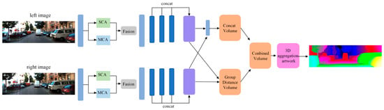
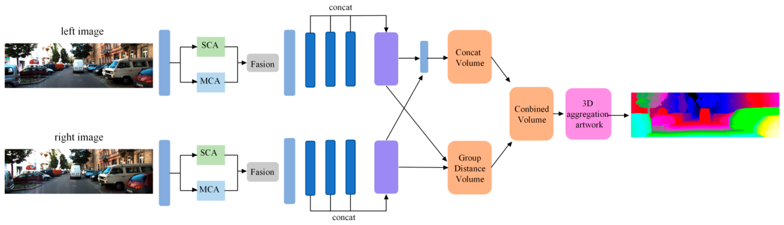
The architecture of the proposed Attention-based Grouping Distance Stereo Network is shown in Figure 1. The network consists of a feature extractor with SCA and MCA modules, grouping distance volume, and a 3D aggregation network. Unlike the attention mechanism in the aforementioned stereo matching methods, the proposed SCA and MCA modules in this paper are used in feature extraction. On the one hand, the SCA module captures more contextual information in a non-local manner and effectively addresses matching ambiguity in large weak texture regions. On the other hand, MCA calibrates feature channels from multiple different subspaces and improves the robustness of the feature representation. The highly discriminative features can be obtained by fusing the SCA and MCA modules. Furthermore, we construct a grouping distance volume by calculating the grouping distance of features between left and right images. This not only preserves more similarity information but also reduces the size of the cost volume.

Figure 1. Architecture overview of the proposed AGDNet.

3.1. Network Architecture

For feature extraction, a pair of stereo images is input, and three 3 × 3 convolution filters are initially used to construct a deeper network and extract image deep features with the consistent receptive field. The extracted features are then input into the SCA and MCA module in parallel, aiming to obtain improved global and local features and enhance contextual semantic associations for generating feature maps with stronger representation capabilities. The outputs obtained from the two modules are fused at the next operation. Afterwards, the basic residuals blocks [28] are used to learn the unary feature extraction. To expand the receptive field further, dilated convolutions are applied in the fourth layer. The last three layers of feature maps are concatenated to form 320-channel unary feature maps.

The cost volume consists of two parts, i.e., a grouping distance volume and a concatenation volume. The concatenation volume follows the same approach as PSMNet [11] that concatenate the left and right features directly. To reduce computational cost, we employ two convolutional layers to compress the unary feature channels to 12. Moreover, our proposed grouping distance volume diminishes the dimension of the feature vectors while retaining crucial information, as elaborated in Section 3.4. Subsequently, the two cost volumes are concatenated and used as the input of the 3D aggregation network.

For cost aggregation, the network contains a pre-hourglass module and three stacked 3D hourglass structures, which are responsible for generating disparity maps and regularizing the cost volume, similar to GWCNet [12]. The pre-hourglass module comprises four 3D convolutions, followed by the application of ReLU and batch normalization. Each stacked 3D hourglass module utilizes four 3 × 3 × 3 3D convolutions in the encoding part and further adopts two 3 × 3 × 3 3D deconvolutions to restore the original resolution in the decoding part. The pre-hourglass module and three stacked 3D hourglass networks are connected to the output module, each of which generates a disparity map. The loss function is described in Section 3.5.

3.2. Spatial Criss-Cross Attention Module

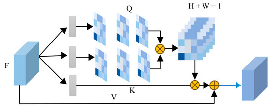
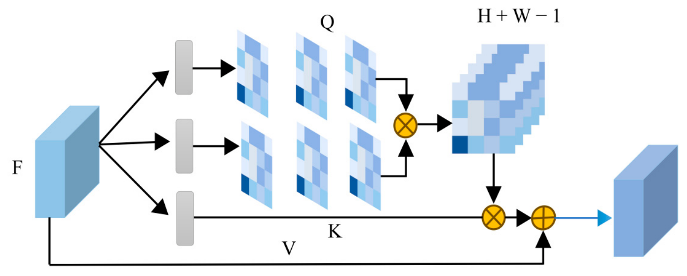
In order to enhance the semantic discrimination ability of features, it is necessary to mine the semantic correlation between pixels through spatial attention mechanisms. However, non-local attention comes with significant computational overhead O((H × W) × (H × W)), making it impractical for larger input images. As such, inspired by CCNet [29] in the field of semantic segmentation, we propose a spatial criss-cross attention module (SCA) so as to construct the non-local information dependence between pixels. The architecture of the SCA module is illustrated in Figure 2.

Figure 2. The architecture of the SCA module.

Firstly, given an input feature map F ∈ R^C×H×W, where C represents the number of channels in the feature map and H, W represent its height and width, respectively. Two 1 × 1 convolutions are used to reduce the dimension of the channel and generate two new feature maps Q and K, where $\left\{Q,K\right\}\in R^{C^{\prime }\times H\times W}$ and C^′ is set to C/8 for reducing computational cost. The feature maps Q and K are then used to compute the incidence matrix A∈ R^{(H+W−1)×H×W} through an affinity operation. For feature map Q, we can get a vector $Q_{\mu }\in R^{C^{\prime } }$ from each position μ in the spatial dimension. For feature map K, we can extract H + W − 1 feature vectors for $K_{\mu }\in R^{(H+W-1)\times C^{\prime } }$ in the same column or row with position μ. Then, the i-th element of K_μ is represented as $K_{i,\mu }\in R^{C^{\prime } }$. The affinity calculation formula is as follows:

$$d_{i,\mu } = Q_{\mu }{K}_{i,\mu }^T$$

(1)

where d_i,μ ∈ D represents the degree of correlation between feature Q_μ and K_i,μ (i = [1, …, H + W − 1], D ∈ R^{(H+W−1)×H×W}). By applying the Softmax operation on D over the channel dimension, we can obtain the attention map A. Its element a_i,μ represents the degree of correlation between position μ in the horizontal direction and position i in the vertical direction, which can be represented as:

$$a_{i,\mu }={\displaystyle \frac{\exp \left(d_{i,\mu }\right)}{{\displaystyle {\sum }_{i=1}^{H+W-1}}\exp \left(d_{i,\mu }\right)}}$$

(2)

At the same time, we input the original feature map F into an additional convolutional layer with a 1 × 1 filter to generate V ∈ R^C×H×W. For the feature map V, we can obtain V_i,μ ∈ R^(H+W−1)×C in the same column or row with position μ. The final output Y_μ is collected by the following operation:

$$Y_{\mu }=\alpha {\displaystyle {\sum }_{i=1}^{H+W-1}}{(a}_{i,\mu }{V}_{i,\mu })+F_{\mu }$$

(3)

where α is a learnable factor. The context information is added to the new feature map Y_μ by a residual module.

By our design, the SCA module assigns higher weights to pivotal locations. It also can be seen that the final output effectively utilizes the non-local information dependence and strengthens the capability of feature representation.

3.3. Multi-Head Channel Attention Module

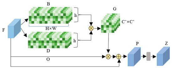
The varying semantic responses among channel maps of each high-level feature are interrelated. By exploiting the interdependencies between these channel maps, we can dynamically modulate the significance of each channel, thereby enhancing the model’s ability to leverage the information within the input images more effectively. In this paper, the multi-head attention strategy is introduced into the channel attention module, which can extract information from multiple subspaces and further obtain feature maps with a stronger ability of representation. The Multi-head Channel Attention module (MCA) facilitates multiple attention calculations in parallel by reconstructing the feature maps and dividing query, key, and value into h heads. Each attention head can focus on distinct features and context; therefore, the model can capture richer information and enhance the ability of representation and expressiveness. The MCA module is shown as Figure 3.

Figure 3. The architecture of the MCA module.

Given an input feature map F ∈ R^C×H×W, it is reconstructed and flattened to one dimension in the spatial dimension; the new feature maps consist of C channel vectors of (H × W) length and are further grouped according to the presuppose number of h heads (h = 4 in this paper), in which each group contains C′ channels (C = h × C’). And from that, we can obtain $\{B,D\}\in R^{h\times C^{\prime }\times \mathit{HW}}$. We take the m-th head as an example, vector B_v,m ∈ R^HW, representing the flattened feature map B in the v-th channel of the m-th head. C′ vectors can be extracted in the m-th head of the feature map D and then are used to form $D_m\in R^{C^{\prime }\times \mathit{HW}}$; the j-th channel in D_m is represented as vector D_j,m ∈ R^HW. The affinity calculation formula is as follows:

$$s_{j,v,m} = B_{v,m}{D}_{j,m}^T$$

(4)

where s_j,v,m represents the degree of correlation between channel v and channel j in the m head. Thus, in the m-th head, the degree of correlation between channel v and all channels is

$$S_{v,m}=B_{v,m}{D}_m^T$$

(5)

where $S_{v,m}\in R^{C^{\prime }}$ and the degree of correlation between all channels in m head can be expressed as $S_m\in R^{C^{\prime }\times C^{\prime }}$. Furthermore, the degree of correlation between all channels in all heads is represented by the matrix $S\in R^{{h\times C}^{\prime }\times C^{\prime }}$. Then, the Softmax operation is applied along the channel dimension for each head of matrix S, and the correlation matrix $G\in R^{{h\times C}^{\prime }\times C^{\prime }}$ can be obtained. By reconstructing the feature map F and dividing it into h group, $O\in R^{h\times C^{\prime }\times \mathit{HW}}$ can be obtained. We can obtain $O_m\in R^{ C^{\prime }\times \mathit{HW}}$ which is the m-th head of the matrix O. Similarly, we can also obtain G_m∈ which is the m-th head of the correlation matrix G. We can apply attention to all vectors in the m-th head by the following calculation:

H_m = G_mO_m

(6)

where $H_m\in R^{C^{\prime }\times \mathit{HW}}$; we repeat the above operation on each head and concatenate them to obtain the feature map P ∈ R^C×H×W. Linear projection W ∈ R^C×C is applied to feature map P, which is then multiplied by a scalar β that is self-learned and initially set to 0. The final output Z ∈ R^C×H×W is obtained by the following calculative process:

Z = βWP + F

(7)

Through the above calculations, we implement the multi-head attention mechanism in the channel dimension. With this design, each head can focus on different channel subspaces of the input. More representational channels are effectively enhanced and irrelevant channels are suppressed.

3.4. Grouping Distance Volume

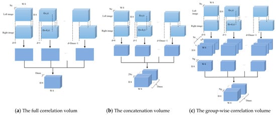
Previous approaches in stereo matching utilized methods such as full correlation volume [10], concatenation volume [30], and group-wise correlation volume [12] to construct the cost volume from left and right features. However, these methods suffer from several drawbacks. It is shown in Figure 4a, where the full correlation only generates a single-channel correlation map for each disparity level, resulting in the loss of multi-channel relevant matching information. The 4D cost volume [12,30] offers several advantages compared with 3D cost volume [10]. It is evident from Figure 4b. The additional channel dimension expands the range of disparity choices, enabling more precise depth estimation. Moreover, the 4D cost volume preserves correlation information between each pixel and all disparity values. This retention of available information among feature pixels enhances the accuracy of disparity estimation. However, the concatenation volume lacks the similarity information between left and right features, necessitating the learning of similarity from scratch in the 3D cost aggregation network, which requires additional parameters. As shown in Figure 4c, the group-wise correlation volume can extract the multi-channel matching feature information, but it solely relies on the inner product operation between the left and right feature groups. Therefore, only when the feature vectors are unit vectors can the correlation operation accurately measure the similarity of the features; otherwise, it will cause a lot of errors in the similarity and inaccurate disparity calculation.

Figure 4. The structure of the cost volume.

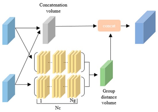
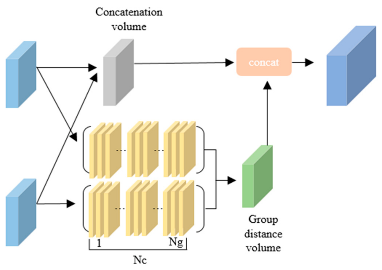
To address the above problems, this work proposes a method to construct the cost volume based on measuring grouping distance. This approach reduces the dimension of the feature vectors while preserving the available information within it. Different from the inner product operation used in the group-wise correlation method, the grouping distance method utilizes L2 distance to calculate the similarity between the left and right feature groups. Furthermore, the final cost volume consists of two components: a concatenation volume and a grouping distance volume. The architecture of constructing our cost volume is illustrated in Figure 5.

Figure 5. The structure of the grouping distance volume.

The left and right feature maps outputted by the feature extractor are denoted as f_l and f_r, respectively. When the size of the input images is H × W, the size of the generated feature maps is [3 × Nc × H/4 × W/4], where N_c = 320 represents the channel number of the feature maps. In this study, for the feature vector f_l(x,y) on the left feature image f_l, under the disparity d, its corresponding pixel on the right feature map is f_r(x − d,y). The channels of both the left and right feature vectors are respectively divided into N_g groups along the channel dimension. Each group contains subvectors with N_c/N_g channels. The k-th feature group $f_l^k$, $f_r^k$ consists of the $k{\displaystyle \frac{N_c}{N_g}}$, $k{\displaystyle \frac{N_c}{N_g}}$ + 1, …, $(k+1){\displaystyle \frac{N_c}{N_g}}-1$ -th channels of the original feature f_l and f_r. The grouping distance GD(f_l(x,y),f_r(x − d,y)) of the feature vectors f_l(x,y) and f_r(x − d,y) is defined as

$${\mathit{GD}\left(f_l\left(x,y\right),f_r\left(x-d,y\right)\right)=\left[‖f_l^0,f_r^0‖,‖f_l^1,f_r^1‖,\dots ,‖f_l^{N_g-1},f_r^{N_g-1}‖\right] }^T$$

(8)

where ||·,·|| denotes the L2 distance calculation between two vectors. The resulting GD vector contains more information regarding the similarity between the left pixels and its corresponding right pixels. Accordingly, the matching cost of pixel p under disparity d can be computed using the grouping distance between feature vectors f_l(x,y) and f_r(x − d,y).

C_gdc (x, y, d) = GD(f_l(x,y), f_r(x − d,y))

(9)

where d represents the disparity; the grouping distance between the left feature vectors and the corresponding right feature vectors is calculated under all disparity d. The correlation maps between each group are then obtained and packed into a grouping distance cost volume of dimension [Ng × D_max/4 × H/4 × W/4], where D_max represents the maximum disparity and D_max/4 denotes the maximum disparity for the feature. In addition, we combine the grouping distance cost volume with the concatenation volume to further improve the accuracy of disparity estimation. The experimental results demonstrate that our proposed method outperforms the application of a single cost volume.

3.5. Loss Function

For each pixel, we have a D_max-length vector which contains the probability p for all disparity levels. Furthermore, the disparity estimation $\tilde{d}$ is calculated by the soft argmin function [30],

$$\tilde{d}={\displaystyle {\sum }_{k=0}^{\mathrm{Dmax}-1}}k·p_k$$

(10)

where k and p_k represent a possible disparity level and the corresponding probability. Since the 3D cost aggregation network has four outputs which are $\tilde{d}0$, $\tilde{\mathrm{d}}$1, $\tilde{\mathrm{d}}$2, and $\tilde{\mathrm{d}}$3, the final loss is calculated by

$$L={\displaystyle {\sum }_{i=0}^3}{\lambda }_i·{\mathit{Smooth}}_{L_1}(\widetilde{d_i}-d^{\ast })$$

(11)

where λ_i represents the coefficients for the i-th disparity prediction and d^∗ denotes the ground truth disparity map.

The smooth L₁ loss is given by

$${\mathit{Smooth}}_{L_1}(x)=\left\{\begin{array}{c}0.5x^2, \mathit{if}\left|x\right|<1\\ \left|x\right|-0.5, \mathit{otherwise}\end{array}\right.$$

(12)

4. Experimental Results

4.1. Experimental Setup

In this section, we evaluate our AGDNet on the Scene Flow [10] dataset, KITTI stereo 2015 [31], and KITTI stereo 2012 [2] datasets. The Scene Flow dataset is a dataset collection of synthetic stereo datasets and provides dense ground truth disparity maps. The Scene Flow dataset includes 35,454 training and 4370 testing images. The size of all images in this dataset is 960 × 540. KITTI 2012 and KITTI 2015 are datasets designed for driving scene analysis. The KITTI 2012 dataset utilizes binocular cameras mounted on car rooftops to capture stereo images of outdoor scenes. KITTI 2015 dataset is extensively used for binocular stereo matching algorithms. The KITTI 2012 dataset provides 194 training image pairs and 195 testing image pairs, while the KITTI 2015 dataset provides 200 training image pairs and 200 testing image pairs.

Our AGDNet was implemented using PyTorch 2.4.0. The model uses the Adam optimizer [32] with β1 = 0.9 and β2 = 0.999. We trained our model on two NVIDIA GeForce RTX 4090 GPUS (CUDA 12.4), and all images were randomly cropped to a size of 256 × 512. For the Scene Flow dataset, we trained our network for 40 epochs with a batch size of 6. The initial learning rate was set to 0.001; after the 10, 15, 20, 25, 30, 32, 34, 36, 38 epochs, it was decayed by a factor of 2. We set the maximum disparity size of the cropped images as D_max = 192 according to the method of PSMNet.

For the KITTI 2015 dataset and KITTI 2012 dataset, we fine-tuned our model pretrained on the Scene Flow dataset for 300 epochs. The initial learning rate was set to 0.001 and scaled down by 10 at the 200-th epoch.

4.2. Evaluation on the Scene Flow Dataset

For the Scene Flow dataset, the metric end-point error (EPE) was usually used to evaluate our network, which is the average disparity error in pixels. We compared the accuracy of AGDNet with other methods on Scene Flow dataset. As shown in Table 1, our method outperforms other methods in terms of accuracy and achieves state-of-the-art performance. We can observe that our AGDNet improves EPE by 8.4% on the Scene Flow dataset compared with HCVNet [33].

Table 1. Performance comparison of AGDNet with other methods on Scene Flow datasets.

Method	GWCNet [12]	EASNet [13]	AANet [14]	CFNet [15]	HybridNet [18]	ESNet [20]	HCVNet [33]	SFFNet [34]	MSFFNet [35]	Ours
EPE (px)	0.76	0.72	0.87	0.97	0.72	0.95	0.71	1.04	1.01	0.65

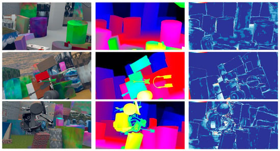
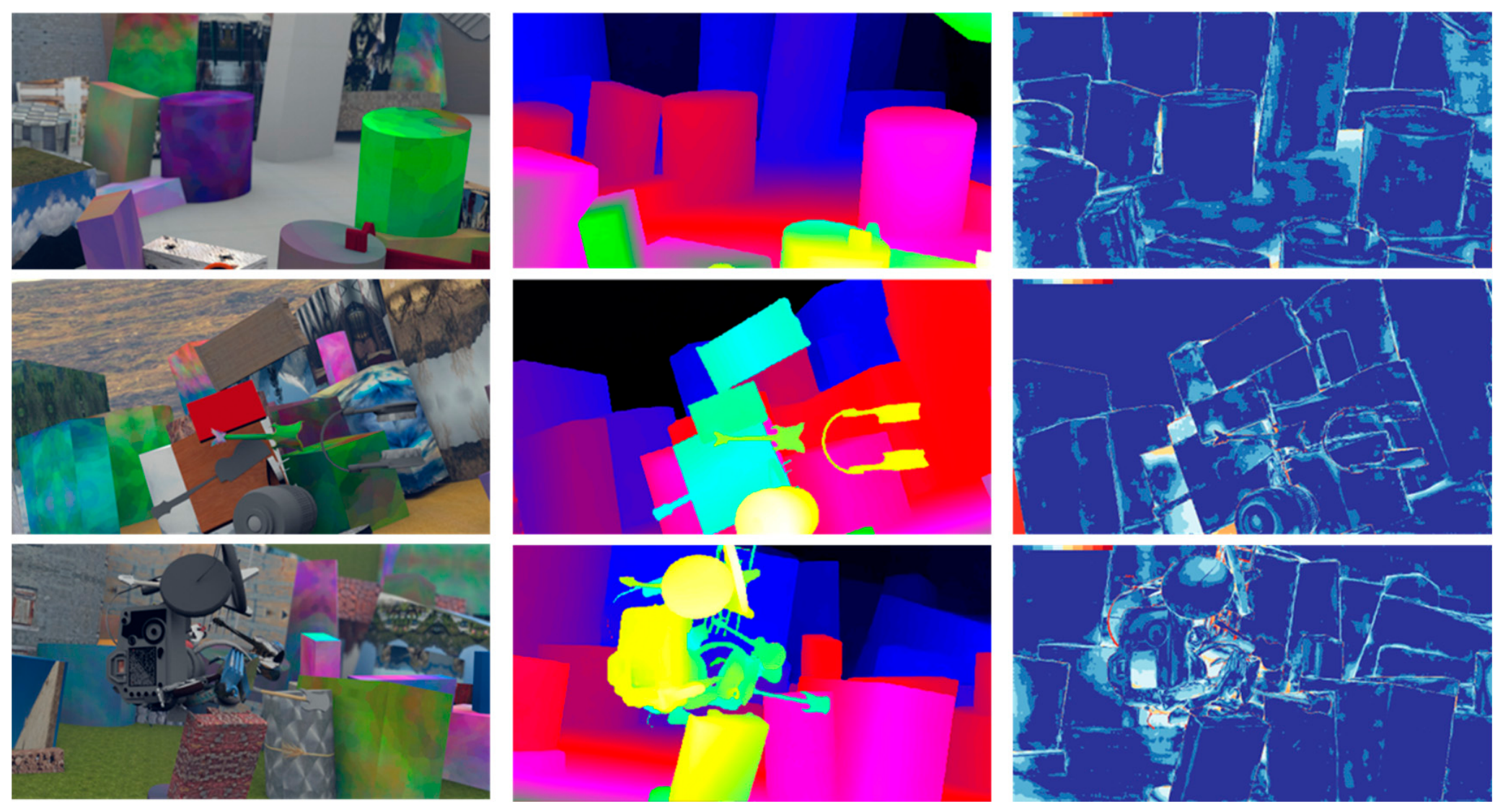
In addition to qualitative evaluation, we conducted a qualitative analysis on the Scene Flow dataset. Figure 6 illustrates the results of the validation set, which consist of left images, predicted disparity maps by pseudo-color treatment, and error maps. As shown in the error maps of Figure 6, The disparity maps generated by our AGDNet are very smooth and have few pixels with large disparity errors, particularly in ill-posed regions. The results demonstrate that our AGDNet can not only notably reduce the error rate on the large textureless and occluded regions but also maintain the shape and structure of the object well.

Figure 6. Visualization results of the Scene Flow test dataset. From left: input left images, predicted disparity maps, error maps.

4.3. Evaluation on the KITTI Benchmark

To evaluate our AGDNet, we compare our model with other state-of-the-art methods on the KITTI datasets. For KITTI 2015 dataset, we submit our results on the KITTI 2015 test dataset to the KITTI evaluation server, and the evaluation results on the test dataset are shown in Table 2. The accuracy is measured by the percentage of pixels whose disparity error is greater than 3px (i.e., D1) on the test dataset. In this table, “All” means that all pixels were considered in error estimation, whereas “Noc” means that only the pixels in non-occluded regions were taken into account. The three columns “D1-bg”, “D1-fg”, and “D1-all” mean the pixels in the background, foreground, and all areas, respectively. As shown in Table 2, the overall three-pixel error of the proposed AGDNet is 2.22% and the overall matching accuracy of our method is superior to other methods in the table.

Table 2. Comparison with other methods on the KITTI 2015 test dataset.

Methods	Noc (%)			All (%)
	D1-bg	D1-fg	D1-All	D1-bg	D1-fg	D1-All
PSMNet [11]	1.71	4.31	2.14	1.86	4.62	2.32
AANet [14]	1.80	4.93	2.32	1.99	5.39	2.55
HybridNet [18]	-	-	-	1.93	-	2.42
ESNet [20]	-	-	-	2.29	4.17	2.60
FADNet [36]	2.35	2.61	2.39	2.50	3.10	2.60
Self-SuperFlow-ft [37]	3.40	7.71	4.11	3.81	8.92	4.66
StereoVAE [38]	3.88	8.94	4.71	4.25	10.18	5.23
P3Snet+ [39]	3.86	6.66	4.32	4.15	7.59	4.72
SFFNet [34]	2.50	5.44	2.99	2.69	6.23	3.28
MSFFNet [35]	2.35	4.58	2.72	2.53	4.99	2.94
DPDNet_2D [40]	1.74	4.67	2.23	1.91	5.29	2.47
SARNet [41]	1.69	4.09	2.09	1.87	4.45	2.30
Ours	1.63	3.93	2.01	1.77	4.44	2.22

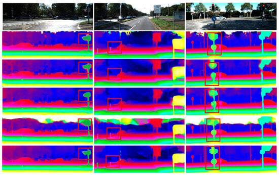
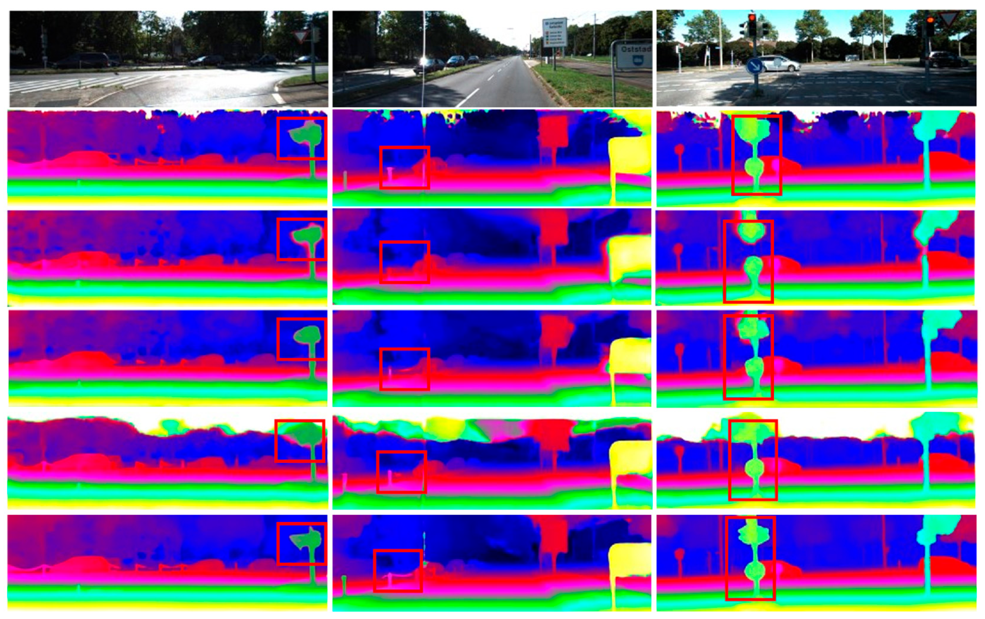
We also conduct qualitative analysis on the KITTI 2015 dataset. Figure 7 shows the qualitative analysis of the KITTI 2015 dataset, including input left images, false color disparity maps predicted by FADNet [36], Self-SuperFlow-ft [37], StereoVAE [38] and P3Snet+ [39], and false color disparity maps predicted by our AGDNet. As shown in Figure 7, our proposed method can obtain higher-quality disparity maps. The edges and fine structures of objects in the disparity map can be well preserved, and the matching ambiguity of large areas of weak texture such as road surfaces has been effectively eliminated.

Figure 7. Results of disparity estimation for KITTI 2015 test images. From top: input left images, results of FADNet [36], results of Self-SuperFlow-ft [37], results of StereoVAE [38], results of P3Snet+ [39], and results of our AGDNet.

For the KITTI 2012 dataset, the accuracy is measured by the percentage of pixels whose disparity error is greater than 2 px, 3 px, and 5 px, respectively, and end-point error (EPE) for non-occluded (Noc) and all (All) pixels. We submit our disparity results of the KITTI 2012 test dataset to the KITTI evaluation server. The evaluation results on the test dataset are shown in Table 3. It can be observed that the EPE of all methods in Table 3 are roughly equivalent. Although the running time of our method is slightly longer, the proposed method has the lowest error rate, and its average three-pixel error of all pixels is 1.66%. On the whole, our method can achieve a better balance between accuracy and speed.

Table 3. Comparison with other methods on the KITTI 2012 dataset.

Method	>2 px (%)		>3 px (%)		>5 px (%)		EPE (px)		Runtime (s)	Environment
	Noc	All	Noc	All	Noc	All	Noc	All
PSMNet [11]	2.44	3.01	1.49	1.89	0.90	1.15	0.5	0.6	0.41	Nvidia GTX Titan Xp
GWCNet [12]	2.16	2.71	1.32	1.70	0.80	1.03	0.5	0.5	0.32	GPU @ 2.0 Ghz
AANet [14]	2.90	3.60	1.91	2.42	0.98	1.30	0.5	0.5	0.062	NVIDIA V100 GPU
HCVNet [33]	2.16	2.75	1.31	1.72	0.79	1.05	0.5	0.5	0.26	NVIDIA Tesla V100GPU
DPDNet_2D [40]	2.94	3.67	1.89	2.42	1.11	1.46	0.5	0.6	0.09	GPU @ 2.5 Ghz
SARNet [41]	2.17	2.82	1.38	1.84	0.86	1.15	0.5	0.5	0.01	GPU @ 2.5 Ghz
SGNet [42]	2.22	2.89	1.38	1.85	0.86	1.15	0.5	0.5	0.6	GPU @ 2.5 Ghz
PGNet [43]	2.14	2.81	1.31	1.79	0.82	1.11	0.5	0.5	0.7	GPU @ 2.5 Ghz
Ours	2.03	2.59	1.27	1.66	0.77	1.01	0.5	0.5	0.02	NVIDIA RTX 4090 GPU

4.4. Ablation Study

This paper uses the Scene Flow dataset to conduct ablation experiments and gives quantitative results on the effects of Spatial Criss-Cross Attention module (SCA), Multi-head Channel Attention module (MCA), and grouping distance volume (GD). In order to prove the effectiveness of the proposed modules, we also conducted several experiments on different models. In the Base model, the SCA and MCA modules are removed and the grouping correlation volume (GC) replaces GD. In the Base + GD model, the GD replaces the grouping correlation volume (GC). In the Base + SCA + GC model, the SCA and GC are adopted. In the Base + SCA + MCA + GC model, the MCA is added in Base + SCA + GC. Base + SCA + MCA + GD is actually the proposed ADGNet, as shown in Table 4, where √ means adding.

Table 4. Ablation study of the AGDNet on the Scene Flow dataset.

Model	Component				D1 (%)	EPE (px)
	SCA	MCA	GC	GD
Base			√		2.71	0.76
Base + GD				√	2.65	0.73
Base + SCA + GC	√		√		2.58	0.71
Base + SCA + MCA + GC	√	√	√		2.41	0.69
Base + SCA + MCA + GD	√	√		√	2.30	0.65

In this section, we evaluate the efficacy of our proposed modules. Specifically, we apply the SCA module to establish non-local information dependence between pixels by utilizing the attention mechanism. Additionally, we incorporate the MCA module, which obtains feature maps with stronger capacity of representation by introducing multi-head attention strategy into the channel attention module. These modules effectively enhance the discriminability of features in ill-posed regions. Moreover, we introduce the grouping distance volume (GD) in order to construct a compact cost volume, so that the size of the cost volume is reduced while still retaining all available information.

As indicated by our experiments in Table 4, integrating all three proposed modules yields the best performance, as they are designed to be mutually complementary. The results show that our model with the three modules reduces EPE by 15% on the Scene Flow dataset compared with the Base model.

5. Conclusions

In this paper, we introduce the SCA module and MCA module to fuse channel and cross-attention; the former can make full use of the non-local context information between pixels, and the latter generates feature maps with a stronger capacity of representation. We also propose a new cost volume, named grouping distance volume, which reduces the volume and parameters while preserving the useful matching information. We have verified that our AGDNet has an excellent performance on the Scene Flow dataset, KITTI 2015 dataset, and KITTI 2012 dataset. It is worth noting that cost aggregation and disparity refinement are also crucial steps in stereo matching. In future research, we will explore a more effective cost aggregation method to enhance the discrimination of matching costs and research disparity refinement strategy to further improve the accuracy of disparity maps.

References

- Schmid, K.; Tomic, T.; Ruess, F.; Hirschmuller, H.; Suppa, M. Stereo vision based indoor/outdoor navigation for flying robots. In Proceedings of the IEEE International Conference on Intelligent Robots and Systems, Tokyo, Japan, 3–7 November 2013; pp. 3955–3962. [Google Scholar]
- Geiger, A.; Lenz, P.; Urtasun, R. Are we ready for autonomous driving? The KITTI vision benchmark suite. In Proceedings of the IEEE Conference on Computer Vision and Pattern Recognition, Providence, RI, USA, 16–21 June 2012; pp. 3354–3361. [Google Scholar]
- Wu, W.; Appiah, I.; Hu, R. Advancements in 3-D object detection: A comprehensive review. J. King Saud Univ. Comput. Inf. Sci. 2025, 37, 294. [Google Scholar] [CrossRef] [Scilit]
- Fan, R.; Ai, X.; Dahnoun, N. Road surface 3d reconstruction based on dense subpixel disparity map estimation. IEEE Trans. Image Process. 2018, 27, 3025–3035. [Google Scholar] [CrossRef] [Scilit] [PubMed]
- Bourdy, C. 3D reconstruction and interpretation in human binocular vision by processing of disparity information. J. Opt. 1989, 20, 243. [Google Scholar] [CrossRef] [Scilit]
- Musleh, B.; Martin, D.; Armingol, J.M.; de la Escalera, A. Continuous pose estimation for stereo vision based on UV disparity applied to visual odometry in urban environments. In Proceedings of the IEEE International Conference on Robotics and Automation, Hong Kong, China, 31 May–5 June 2014; pp. 3983–3988. [Google Scholar]
- Scharstein, D.; Szeliski, R. A taxonomy and evaluation of dense two-frame stereo correspondence algorithms. Int. J. Comput. Vis. 2002, 47, 7–42. [Google Scholar] [CrossRef] [Scilit]
- Wu, W.; Zhu, H.; Zhang, Q. Oriented-linear-tree based cost aggregation for stereo matching. Multimed. Tools Appl. 2019, 78, 15779–15800. [Google Scholar] [CrossRef] [Scilit]
- Zhan, Y.; Gu, Y.; Huang, K.; Zhang, C.; Hu, K. Accurate image-guided stereo matching with efficient matching cost and disparity refinement. IEEE Trans. Circuits Syst. Video Technol. 2015, 26, 1632–1645. [Google Scholar] [CrossRef] [Scilit]
- Mayer, N.; Ilg, E.; Hausser, P.; Fischer, P.; Cremers, D.; Dosovitskiy, A.; Brox, T. A large dataset to train convolutional networks for disparity, optical flow, and scene flow estimation. In Proceedings of the IEEE Conference on Computer Vision and Pattern Recognition, Las Vegas, NV, USA, 27–30 June 2016; pp. 4040–4048. [Google Scholar]
- Chang, J.R.; Chen, Y.S. Pyramid stereo matching network. In Proceedings of the IEEE Conference on Computer Vision and Pattern Recognition, Salt Lake City, UT, USA, 18–22 June 2018; pp. 5410–5418. [Google Scholar]
- Guo, X.; Yang, K.; Yang, W.; Wang, X.; Li, H. Group-wise correlation stereo network. In Proceedings of the IEEE Conference on Computer Vision and Pattern Recognition, Long Beach, CA, USA, 16–20 June 2019; pp. 3273–3282. [Google Scholar]
- Wang, Q.; Shi, S.; Zhao, K.; Chu, X. EASNet: Searching elastic and accurate network architecture for stereo matching. In Proceedings of the European Conference on Computer Vision, Tel Aviv, Israel, 23–27 October 2022; pp. 437–453. [Google Scholar]
- Xu, H.; Zhang, J. Aanet: Adaptive aggregation network for efficient stereo matching. In Proceedings of the IEEE Conference on Computer Vision and Pattern Recognition, Virtual, 14–19 June 2020; pp. 1959–1968. [Google Scholar]
- Shen, Z.; Dai, Y.; Rao, Z. Cfnet: Cascade and fused cost volume for robust stereo matching. In Proceedings of the IEEE Conference on Computer Vision and Pattern Recognition, Nashville, TN, USA, 21–25 June 2021; pp. 13906–13915. [Google Scholar]
- Yang, G.; Manela, J.; Happold, M.; Ramanan, D. Hierarchical deep stereo matching on high-resolution images. In Proceedings of the IEEE Conference on Computer Vision and Pattern Recognition, Long Beach, CA, USA, 16–20 June 2019; pp. 5515–5524. [Google Scholar]
- Ronneberger, O.; Fischer, P.; Brox, T. U-net: Convolutional networks for biomedical image segmentation. In Proceedings of the 18th International Conference on Medical Image Computing and Computer-assisted Intervention, Munich, Germany, 5–9 October 2015; pp. 234–241. [Google Scholar]
- Gan, W.; Wu, W.; Chen, S.; Zhao, Y.; Wong, P.K. Rethinking 3D cost aggregation in stereo matching. Pattern Recognit. Lett. 2023, 167, 75–81. [Google Scholar] [CrossRef] [Scilit]
- Sun, D.; Yang, X.; Liu, M.-Y.; Kautz, J. Pwc-net: Cnns for optical flow using pyramid, warping, and cost volume. In Proceedings of the IEEE Conference on Computer Vision and Pattern Recognition, Salt Lake City, UT, USA, 18–22 June 2018; pp. 8934–8943. [Google Scholar]
- Huang, Z.; Norris, T.B.; Wang, P. ES-Net: An efficient stereo matching network. arXiv 2021, arXiv:2103.03922. [Google Scholar]
- Zhang, Y.; Li, Y.; Wu, C.; Liu, B. Attention-guided aggregation stereo matching network. Image Vis. Comput. 2021, 106, 104088. [Google Scholar] [CrossRef] [Scilit]
- Li, X.; Fan, Y.; Lv, G.; Ma, H. Area-based correlation and non-local attention network for stereo matching. Vis. Comput. 2022, 38, 3881–3895. [Google Scholar] [CrossRef] [Scilit]
- Xu, G.; Cheng, J.; Guo, P.; Yang, X. Attention concatenation volume for accurate and efficient stereo matching. In Proceedings of the IEEE Conference on Computer Vision and Pattern Recognition, New Orleans, LA, USA, 19–24 June 2022; pp. 12981–12990. [Google Scholar]
- Chen, B.; Chen, X.; Zheng, C.; Wu, S. ML-Stereo: Multi-Range Lookup for Stereo Matching. IEEE Trans. Consum. Electron. 2026, 72, 2960–2972. [Google Scholar] [CrossRef] [Scilit]
- Xu, G.; Wang, X.; Ding, X.; Yang, X. Iterative geometry encoding volume for stereo matching. In Proceedings of the IEEE Conference on Computer Vision and Pattern Recognition, Vancouver, BC, Canada, 18–22 June 2023; pp. 21919–21928. [Google Scholar]
- Li, Z.; Liu, X.; Drenkow, N.; Ding, A.; Creighton, F.X.; Taylor, R.H.; Unberath, M. Revisiting stereo depth estimation from a sequence-to-sequence perspective with transformers. In Proceedings of the IEEE International Conference on Computer Vision, Montreal, QC, Canada, 11–17 October 2021; pp. 6197–6206. [Google Scholar]
- Vaswani, A.; Shazeer, N.; Parmar, N.; Uszkoreit, J.; Jones, L.; Gomez, A.N.; Kaiser, Ł.; Polosukhin, I. Attention is all you need. In Proceedings of the 31st International Conference on Neural Information Processing Systems, Long Beach, CA, USA, 4–9 December 2017; Available online: https://papers.nips.cc/paper_files/paper/2017/hash/3f5ee243547dee91fbd053c1c4a845aa-Abstract.html (accessed on 12 September 2026).
- He, K.; Zhang, X.; Ren, S.; Sun, J. Deep residual learning for image recognition. In Proceedings of the IEEE Conference on Computer Vision and Pattern Recognition, Las Vegas, NV, USA, 27–30 June 2016; pp. 770–778. [Google Scholar]
- Huang, Z.; Wang, X.; Huang, L.; Wei, Y.; Liu, W. Ccnet: Criss-cross attention for semantic segmentation. In Proceedings of the IEEE International Conference on Computer Vision, Seoul, Republic of Korea, 27 October–2 November 2019; pp. 603–612. [Google Scholar]
- Kendall, A.; Martirosyan, H.; Dasgupta, S.; Henry, P.; Kennedy, R.; Bachrach, A.; Bry, A. End-to-end learning of geometry and context for deep stereo regression. In Proceedings of the IEEE International Conference on Computer Vision, Venice, Italy, 22–29 October 2017; pp. 66–75. [Google Scholar]
- Menze, M.; Geiger, A. Object scene flow for autonomous vehicles. In Proceedings of the IEEE Conference on Computer Vision and Pattern Recognition, Boston, MA, USA, 7–12 June 2015; pp. 3061–3070. [Google Scholar]
- Kinga, D.; Adam, J.B. A method for stochastic optimization. In Proceedings of the International Conference on Learning Representations (ICLR), San Diego, CA, USA, 7–9 May 2015; Volume 5, p. 1. [Google Scholar]
- Dai, C.; Chang, Q.; Qiu, T.; Liu, X.; Cui, Y. HCVNet: Binocular stereo matching via hybrid cost volume computation module with attention. IEEE Access 2022, 10, 93062–93073. [Google Scholar] [CrossRef] [Scilit]
- Jeong, J.; Jeon, S.; Heo, Y.S. An efficient stereo matching network using sequential feature fusion. Electronics 2021, 10, 1045. [Google Scholar] [CrossRef] [Scilit]
- Jeon, S.; Heo, Y.S. Efficient multi-scale stereo-matching network using adaptive cost volume filtering. Sensors 2022, 22, 5500. [Google Scholar] [CrossRef] [Scilit] [PubMed]
- Wang, Q.; Shi, S.; Zheng, S.; Zhao, K.; Chu, X. Fadnet: A fast and accurate network for disparity estimation. In Proceedings of the IEEE International Conference on Robotics and Automation, Virtual, 31 May–5 June 2020; pp. 101–107. [Google Scholar]
- Bendig, K.; Schuster, R.; Stricker, D. Self-superflow: Self-supervised scene flow prediction in stereo sequences. In Proceedings of the 2022 IEEE International Conference on Image Processing (ICIP), Bordeaux, France, 16–19 October 2022; pp. 481–485. [Google Scholar]
- Chang, Q.; Li, X.; Xu, X.; Liu, X.; Li, Y.; Miyazaki, J. StereoVAE: A lightweight stereo-matching system using embedded GPUs. In Proceedings of the IEEE International Conference on Robotics and Automation, London, UK, 29 May–2 June 2023; pp. 1982–1988. [Google Scholar]
- Emlek, A.; Peker, M. P3SNet: Parallel Pyramid Pooling Stereo Network. IEEE Trans. Intell. Transp. Syst. 2023, 24, 10433–10444. [Google Scholar] [CrossRef] [Scilit]
- Liu, J.; Zhang, Y. DPDNet: The lightweight stereo matching network based on disparity probability distribution consistency. Image Vis. Comput. 2025, 163, 105771. [Google Scholar] [CrossRef] [Scilit]
- Liang, B.; Wang, Y.; Hu, Z.; Huang, Z.; Hu, H.; Xu, J.; Chen, D. High-Precision Stereo Matching Based on Selective Attention and Residual Cost Aggregation for Real-Time Autonomous Driving on Edge Devices. IEEE Trans. Veh. Technol. 2026, 75, 19463–19473. [Google Scholar] [CrossRef] [Scilit]
- Chen, S.; Xiang, Z.; Qiao, C.; Chen, Y.; Bai, T. SGNet: Semantics guided deep stereo matching. In Proceedings of the Asian Conference on Computer Vision, Virtual, 30 November–4 December 2020; pp. 1–17. [Google Scholar]
- Chen, S.; Xiang, Z.; Qiao, C.; Chen, Y.; Bai, T. PGNet: Panoptic parsing guided deep stereo matching. Neurocomputing 2021, 463, 609–622. [Google Scholar] [CrossRef] [Scilit]
Disclaimer/Publisher’s Note: The statements, opinions and data contained in all publications are solely those of the individual author(s) and contributor(s) and not of MDPI and/or the editor(s). MDPI and/or the editor(s) disclaim responsibility for any injury to people or property resulting from any ideas, methods, instructions or products referred to in the content. |
© 2026 by the authors. Licensee MDPI, Basel, Switzerland. This article is an open access article distributed under the terms and conditions of the Creative Commons Attribution (CC BY) license.