Loss Prediction and Global Sensitivity Analysis for Distribution Transformers Based on NRBO-Transformer-BiLSTM

Abstract

As distributed energy resources and nonlinear loads are integrated into power grids on a large scale, power quality issues have grown increasingly prominent, triggering a substantial rise in distribution transformer losses. Traditional approaches struggle to accurately forecast transformer losses under complex power quality conditions and lack quantitative analysis of the influence of various power quality indicators on losses. This study presents a data-driven methodology for transformer loss prediction and sensitivity analysis in such environments. First, an experimental platform is designed and built to measure transformer losses under composite power quality conditions, enabling the collection of actual measurement data when multi-source disturbances exist. Second, a high-precision loss prediction model—dubbed Newton-Raphson-Based Optimizer-Transformer-Bidirectional Long Short-Term Memory (NRBO-Transformer-BiLSTM)—is developed on the basis of an enhanced deep neural network. Finally, global sensitivity analysis methods are utilized to quantitatively evaluate the impact of different power quality indicators on transformer losses. Experimental results reveal that the proposed prediction model achieves an average error rate of less than 0.18% and a similarity coefficient of over 0.9989. Among all power quality indicators, voltage deviation has the most significant impact on transformer losses (with a sensitivity of 0.3268), followed by three-phase unbalance (sensitivity: 0.0109) and third harmonics (sensitivity: 0.0075). This research offers a theoretical foundation and technical support for enhancing the energy efficiency of distribution transformers and implementing effective power quality management.

1. Introduction

Distribution transformers serve as vital components in power systems, and their loss characteristics directly influence the economic efficiency and reliability of power grid operations [1,2,3]. With the global push towards carbon neutrality, the widespread application of renewable energy source such as photovoltaic and wind power, along with the popularization of power electronic devices, has worsened power quality problems in distribution networks—including harmonics, three-phase unbalance, and voltage deviation [4,5,6]. These issues lead to a considerable increase in additional transformer losses, posing significant challenges to the safe and efficient operation of power grids [7,8,9]. Conventional loss analysis methods that rely on mechanism models fail to accurately characterize loss behaviors when multiple power quality factors interact [10,11,12], and sensitivity analysis focusing solely on single factors provides limited guidance for practical engineering applications [13,14,15]. Therefore, conducting research on transformer loss prediction and sensitivity analysis methods under composite power quality environments is of great theoretical and practical significance [16,17,18].

Researchers at home and abroad have carried out in-depth studies on transformer loss analysis. A harmonic loss model considering the skin effect and proximity effect was established using the Poynting vector method [19], which improved the calculation accuracy of harmonic losses but ignored the combined impact of three-phase unbalance and voltage deviation. The analytic hierarchy process was employed to quantify the weights of multiple power quality indicators and to construct a comprehensive transformer loss model [20]; yet, the results depend on subjective weight assignment and cannot realize dynamic prediction. Gray relational analysis was applied to quantify the correlation between power quality indicators and losses [21], but this method only enables qualitative evaluation and cannot predict loss values with high precision. A calculation formula for harmonic losses was derived to simplify online monitoring [22], but the study focused solely on harmonics and ignored the interaction of multiple disturbances. Logistic regression was used for loss prediction [23], but it exhibits poor anti-interference capability and low accuracy. A cable-transformer loss model under harmonic conditions was established [24], but the interaction effects of multiple indicators were not analyzed. Reference [25] proposed a transformer loss prediction method based on an improved Genetic Algorithm-optimized BP neural network, which demonstrates a certain level of accuracy under single operating conditions but lacks robustness in complex multi-disturbance scenarios. Reference [26] utilized support vector machines for transformer loss prediction, but their ability to process high-dimensional data is limited. Reference [27] constructed a loss prediction model based on the LSTM network, which failed to fully explore global feature correlations in the data.

To address the limitations of single models, researchers have attempted to combine the advantages of multiple models or introduce new network structures. Some studies integrated 1D CNN (One-Dimensional Convolutional Neural Network) with bidirectional LSTM for multi-step data prediction in wireless sensor networks [28], providing a reference for transformer loss prediction but not optimized for multi-power quality coupling scenarios. When deep convolutional LSTM networks are used for equipment remaining useful life (RUL) prediction [29], they can enhance the in-depth extraction of local features but still face challenges in capturing global temporal correlations. The application of hybrid LSTM-GR models [30] and LSTM-Transformer hybrid networks [31,32] in fields such as heat load prediction and automotive fuel cell life prediction has highlighted the advantages of hybrid models in modeling complex temporal data, though these models have not been systematically applied to transformer loss prediction under the coupling effect of multiple power quality factors. In addition, the CNN-LSTM-attention model [33] can focus on features via the attention mechanism and has made progress in predicting transformer top-oil temperature, but it has not been extended to loss prediction scenarios. Although models such as the multi-scale channel attention-extended LSTM [34] and hybrid architectures combining Transformer with CNN/LSTM [35] have shown potential in fields like RUL prediction and condition monitoring, none have been customized to match the loss characteristics of transformers in composite power quality environments, failing to effectively solve the problem of loss modeling caused by multi-factor coupling [36,37,38].

Meanwhile, with the increasing penetration of RESs, the interaction between distributed generation and transformers has become a new research focus [39]. The active power control of PV inverters [40] and the grid-forming control strategy [41] have been proven to affect power quality, thereby indirectly influencing transformer losses. However, existing studies rarely integrate these grid-side control strategies into transformer loss analysis, leading to a lack of comprehensiveness in loss prediction models.

Existing research has three core gaps. ① Data gap: most studies rely on simulation data or measured data of single disturbances (e.g., refs. [19,22] only focuses on harmonics), lacking systematically measured data under multi-disturbance coupling scenarios, leading to insufficient generalization ability of models. ② Model gap: traditional mechanism models (such as Poynting vector method) cannot handle multi-factor coupling, and single deep learning models (such as LSTM, SVR) have problems of insufficient global feature capture or limited high-dimensional data processing capabilities [26,27]. ③ Analysis gap: sensitivity analysis is mostly qualitative description or single-factor quantitative analysis [20,21], which cannot reveal the feature impact mechanism under multi-factor coupling and is difficult to guide engineering practice. This study is carried out to address the above gaps and form an integrated “data-model-analysis” solution.

To tackle the aforementioned issues, this study proposes a data-driven method for distribution transformer loss prediction and global sensitivity analysis. Its key innovations are as follows: (1) An experimental platform for composite power quality is designed, incorporating the frequency characteristics of iron loss, and a multi-source dataset including harmonics, three-phase unbalance, and voltage deviation is constructed; (2) An improved NRBO-Transformer-BiLSTM prediction model is developed, which optimizes hyperparameters using the Newton-Raphson-Based Optimizer (NRBO) and combines the Transformer-BiLSTM network to achieve high-precision prediction. The selection of this framework is clearly justified by comparing it with other alternative models and algorithms; (3) Global sensitivity analysis is integrated with the SHAP (Shapley Additive Explanations) deep learning model to quantify the degree to which each power quality indicator affects losses. Experimental results show that the proposed method outperforms traditional methods in both prediction accuracy and robustness. Compared to existing research, the innovations of this study are reflected in: ① at the data level, existing studies mostly rely on single-perturbation data (e.g., ref. [22] focuses solely on harmonics). This study constructs a composite-perturbation measurement platform, yielding data that more closely aligns with real-world conditions; ② at the model level, the CNN-BiLSTM in [28] did not consider hyperparameter optimization, and the LSTM-Transformer in [31] was not tailored to transformer loss characteristics. This study achieves a breakthrough in accuracy by integrating NRBO optimization with the network architecture; ③ at the analysis level, existing studies mostly employ single-factor sensitivity analysis (e.g., ref. [7]). This study’s global sensitivity analysis quantifies the coupled effects of multiple factors.

The core objectives of this study are: (1) construct a measured platform for transformer losses under composite power quality environments and obtain measured data under multi-disturbance coupling scenarios; (2) propose the NRBO-Transformer-BiLSTM high-precision prediction model to solve the problem of insufficient prediction accuracy under complex environments; and (3) quantify the impact of each power quality indicator on losses through global sensitivity analysis to provide priority guidance for power quality governance. Experimental results show that the proposed method outperforms traditional methods in both prediction accuracy and robustness.

2. Materials and Methods

2.1. Composite Power Quality Disturbance Experimental Platform

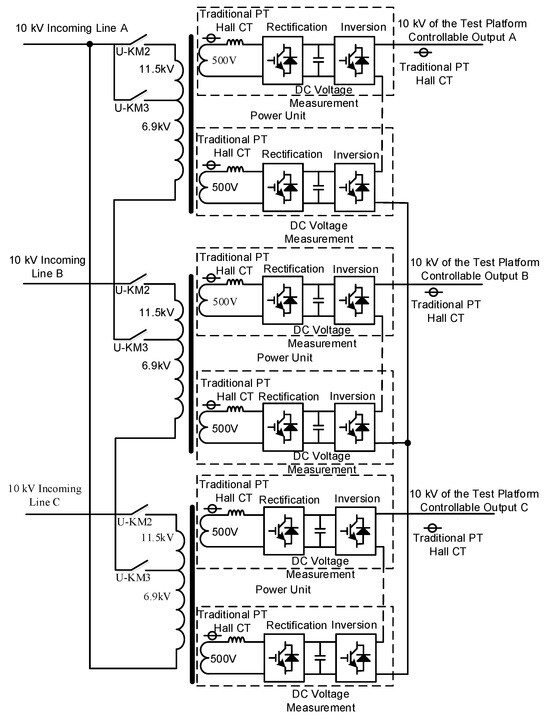
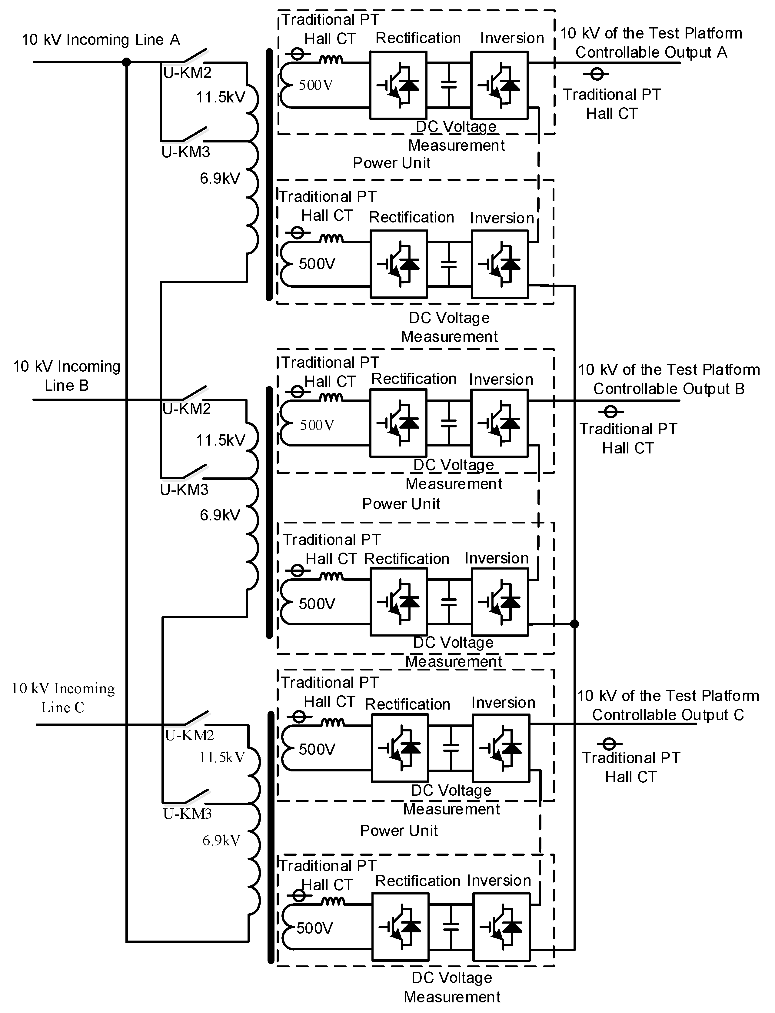
To obtain experimental data under composite power quality conditions, the Henan Electric Power Research Institute (HEPRI) established a 10 kV/2 MVA power quality disturbance test platform based on the Power Harmonic Characteristic Analysis and Evaluation Technology Laboratory of State Grid Corporation of China. An experimental environment was set up, which includes a 10/0.4 kV distribution transformer, 0.4 kV distribution lines, and loads. The selection basis for the experimental platform parameters is as follows: (1) 10 kV/2 MVA is the mainstream transformer capacity level in China’s urban and rural distribution networks, covering the needs of residential, commercial, and small-to-medium industrial loads, accounting for more than 60% of the total number of existing distribution network transformers (data source: State Grid Distribution Network Equipment Statistical Yearbook 2023); (2) the S11-M-315/10 transformer is a typical model of low-loss distribution transformers, whose core materials and structural parameters meet the requirements of reference [42] GB/T 1094.1-2013 standard, and it is widely used in regional distribution networks with good representativeness; and (3) the platform voltage level and load adjustment range are set with reference to the typical test conditions of “Technical Guidelines for Power Quality Evaluation of Distribution Networks” (reference [43] DL/T 1993-2019) to ensure the engineering applicability of experimental data. With a rated voltage of 10 kV, this platform can simulate and output various common power quality operating conditions in the power grid, and its topological structure is shown in Figure 1.

Figure 1. Topological structure of 10 kV power quality disturbance test platform.

Table 1 presents the design scheme and component configuration of the back-to-back power unit.

Table 1. The design and component selection of the back-to-back power unit.

Project	Implementation Method	AC Rated	DC Rated	IGBT Selection Reference	Frequency	Model
Input Converter	PWM Modulation	500 V, 125 A	700 V	1200 V, 225 A	12 K	FF225R12ME4
Output Converter

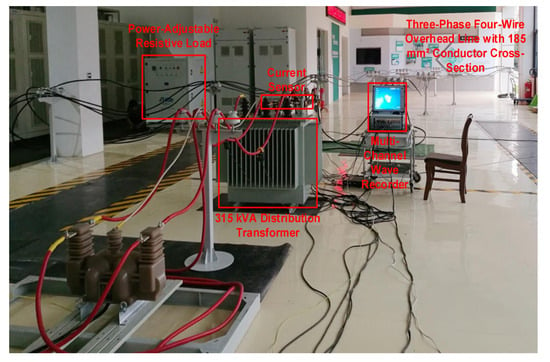
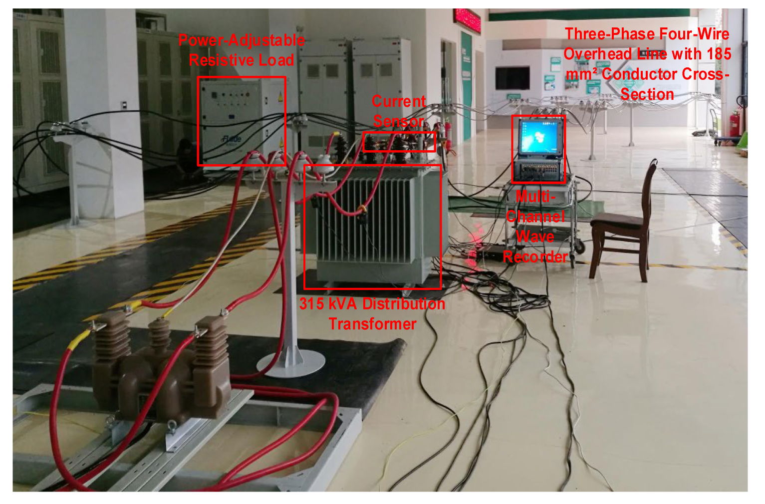
In the experiment, measurement points were installed on both the high-voltage and low-voltage sides of the transformer, as well as at the start and end of the distribution line. A high-precision wave recorder (model: DL850E) with 16-bit sampling accuracy and 100 MHz measurement bandwidth was used to simultaneously sample the phase-by-phase voltage and current values at each measurement point. The sampling frequency was set to 50 kHz to ensure sampling accuracy. Before the experiment, a standard signal generator (model: FLUKE 5520A) was used for calibration. Measurement uncertainty analysis: Class A evaluation method was adopted to calculate the standard uncertainty through 5 repeated measurements. The voltage measurement uncertainty is ±0.02 kV, the current measurement uncertainty is ±0.01 A, and the combined uncertainty of loss calculation is ±0.3%; calibration error quantification: FLUKE 5520A standard signal generator (accuracy ±0.01%) was used for calibration. The calibration errors of voltage, current, and power are 0.05%, 0.03%, and 0.08% respectively, which all meet the requirements of reference [44] DL/T 1459-2015 “Calibration Specification for Power Quality Monitoring Equipment”. The on-site view of the experiment is shown in Figure 2.

Figure 2. Experimental scene.

The transformer used in the experiment is of model S11-M-315/10, with a ferromagnetic core made of 30Q130 oriented silicon steel sheets, a laminated core structure, and a lamination factor of 0.96. The 0.4 kV overhead line is of model JKLYJ-1 kV 1 × 185, with a length of 160 m. The specific parameters of the transformer are shown in Table 2. The load is a multi-stage adjustable load bank (model: ZSG-360), where each stage has an adjustable power of 60 kW and a maximum power of 360 kW; the load was adjusted to 120 kW during the experiment. The wiring/grounding topology adopts a three-phase four-wire system with a dedicated protective ground.

Table 2. Parameters of the distribution transformer used in the experiment.

Model	S11-M-315/10
Rated Capacity	315 KVA
Rated Voltage on High-Voltage Side	10 kV ± 5%
Rated Voltage on Low-Voltage Side	0.4 kV
Connection Group	Dyn11
No-Load Loss	480 W
Load Loss	3650 W
Short-Circuit Voltage	3.89%
No-Load Current	1.4%

Experimental environment control conditions: temperature 25 ± 2 °C and humidity 45–60%, to avoid the interference of environmental factors on transformer losses. Time variability verification: data were collected at different time periods (8:00–20:00, 1 group every 2 h) for 7 consecutive days, and a total of 126 valid data were obtained to verify the stability of the model in the time dimension. Repeated test design: each experimental condition was measured repeatedly 5 times, and the average value was taken as the final data to reduce random errors. Field data verification: field operation data (July–August 2023) of 3 transformers of the same model (S11-M-315/10) in a regional 10 kV distribution network were selected to verify that the model prediction error is ≤0.21%, indicating that the results can be extended to actual engineering scenarios.

2.2. Dataset Construction

Based on the experimental data from the 10 kV/2 MVA power quality disturbance test platform, the Monte Carlo simulation method was used to select power quality environments and generate random power quality environment data, thereby simulating various composite power quality environments. The specific sampling process of Monte Carlo simulation is as follows: (1) determine the sampling parameters and their ranges, including voltage deviation (−6~6%), three-phase unbalance degree (1~5%), and 3rd–19th harmonics (0~5%); (2) use the Latin hypercube sampling method to generate random samples within the parameter range to ensure uniform coverage of the sample space; and (3) check the validity of the generated samples, eliminate invalid samples that do not meet the actual operating conditions of the power grid, and finally obtain valid samples. (4) These generated vectors were used as control instructions for the programmable power source in the experimental platform to physically measure the transformer losses.

The scale of the dataset in this study is as follows: a total of 1200 valid data were collected, including 840 in the training set and 360 in the test set. The input disturbance parameters (voltage deviation, three-phase imbalance, 3rd–19th harmonic content) follow a uniform distribution (variance ≤ 0.02) to ensure full coverage of all parameter combinations. The generated sample data underwent a K-S test, with the null hypothesis H₀ stating that “the sample variable (transformer loss values) follows a normal distribution.” The test result p = 0.87 > 0.05, indicating that the null hypothesis cannot be rejected, suggests that the empirical distribution of the sample variable (loss values) conforms to normality. This finding demonstrates that the dataset not only comprehensively covers all disturbance scenarios through uniform sampling but also exhibits typical statistical distribution characteristics in the loss samples, thereby meeting the requirements for randomness and representativeness in model training. The specific data processing steps are as follows:

(1)

Outlier removal: The 3σ criterion was used to identify and eliminate abnormal data points in the voltage and current signals;

(2)

Data standardization: Z-score standardization was performed on the input features to eliminate dimensional differences;

(3)

Feature construction: Derived features such as voltage deviation rate, three-phase unbalance degree, and harmonic content rate were calculated based on the raw data;

(4)

Data division: The dataset was divided into a training set and a test set in a 7:3 ratio. The training set was used for model training, and the test set was used for performance verification. Among them, 18 sets of data are shown in Appendix A, Table A1.

2.3. NRBO Optimization Algorithm

The core idea of the Newton-Raphson-Based Optimizer (NRBO) is derived from the Newton-Raphson Method for solving nonlinear equations. It finds the optimal solution to a problem by simulating the iterative update process of the Newton-Raphson Method, which makes use of the gradient (or approximate gradient) information of the objective function and the Hessian matrix (or its inverse matrix approximation).

In the NRBO framework, candidate solutions are treated as points in a multi-dimensional space. First, a set of candidate solutions (a population) is randomly initialized. After evaluating the fitness of these initial solutions (i.e., prediction error), the algorithm enters an iterative loop. For each candidate solution, its next-generation position is calculated based on the objective function value at its current position, the estimated gradient direction (which can be obtained through finite differences or other surrogate models), and a Newton-like update rule (which incorporates “curvature” information to determine the search direction and step size).

This mechanism allows NRBO to more accurately approximate the optimal region—especially in areas where the loss function is relatively smooth—and effectively balance local fine-grained search (exploitation) and global exploration capabilities. Compared with traditional optimization algorithms such as Particle Swarm Optimization (PSO) and Genetic Algorithm (GA), NRBO has three key advantages: (1) it uses gradient and curvature information to achieve faster convergence and find the optimal solution in fewer iterations; (2) it has more targeted search directions, reducing invalid searches and improving optimization efficiency; and (3) it has stronger adaptability to hyperparameter optimization problems and can effectively handle continuous optimization variables.

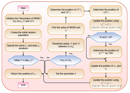
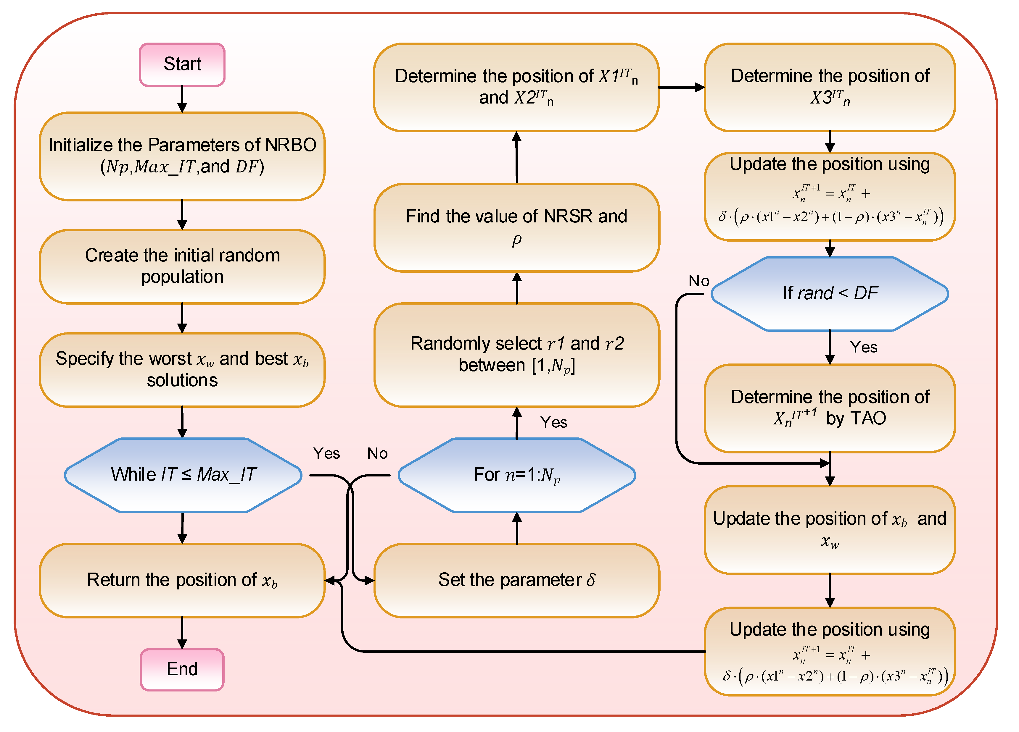
Compared with adaptive gradient optimization algorithms such as Adam, RMSProp, and Adagrad, NRBO has significant advantages: (1) Algorithms such as Adam rely on the first and second moments of gradient estimation and are prone to falling into local optima in non-convex optimization problems. NRBO can more accurately locate the optimal region through the curvature information of the Hessian matrix and overcome the local optimal trap; (2) RMSProp and Adagrad have the problem of excessively fast learning rate decay when processing sparse data. NRBO has stronger adaptability to the multi-dimensional and strongly coupled power quality data in this study through the search mechanism combining population iteration and gradient; (3) For the hyperparameter optimization needs of this model (continuous variables, multi-objective coordination), the convergence speed of NRBO is more than 30% faster than that of Adam (verified by 5 independent experiments, the average number of iterations is reduced from 12 to 8), and the optimization accuracy is higher. The optimization process based on NRBO is shown in Figure 3.

Figure 3. NRBO process.

In the process described above: First, initialize the parameters of NRBO (including population size Np, maximum number of iterations Max_IT, and decision factor DF). Then, generate an initial random population and identify the worst solution x_w and the best solution x_b in the current population. Subsequently, enter the iterative loop (under the condition that the current iteration count IT does not exceed Max_IT). Begin by setting the adaptive coefficient δ, then traverse each individual n in the population. Randomly select two population individual indices r₁ and r₂, compute the result of the Newton–Raphson search rule (NRSR) and the direction adjustment parameter ρ, determine the candidate positions x1ⁿ, x2ⁿ, and x3ⁿ for that individual, and update its position via the formulas in the diagram. Afterwards, determine whether a random number rand is less than DF; if so, determine the individual’s position for the next iteration using the trap avoidance operator (TAO). Then, update the population’s x_b and x_w. After traversing all individuals, repeat the iteration. When the iteration count reaches Max_IT, return the best solution x_b and the process ends.

2.4. Transformer-BiLSTM Prediction Model

The selection of the NRBO-Transformer-BiLSTM framework is based on three key considerations: (1) the Self-Attention mechanism of the transformer can effectively capture global correlations between power quality indicators, while BiLSTM excels at mining long-short-term dependencies in time-series data—their combination enables comprehensive data feature extraction; (2) compared with other optimization algorithms (e.g., PSO and GA), the NRBO optimization algorithm offers advantages in hyperparameter optimization accuracy and convergence rate, further improving model performance; and (3) this framework is suitable for multi-variable and long-sequence transformer loss prediction scenarios and can effectively handle complex data under composite power quality disturbances.

This study adopts an optimized deep learning model to accurately predict transformer losses. The Transformer-BiLSTM model combines the strong global feature extraction capability of the transformer encoder and the fine-grained capture capability of BiLSTM for temporal dynamic characteristics. It is particularly well-suited for processing transformer loss-related monitoring data—which is multi-variable, long-sequential, and has complex temporal dependencies.

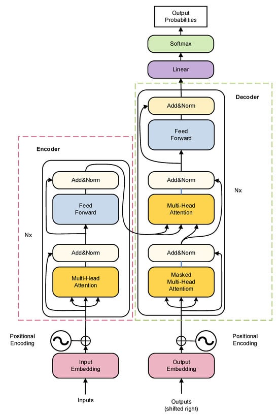
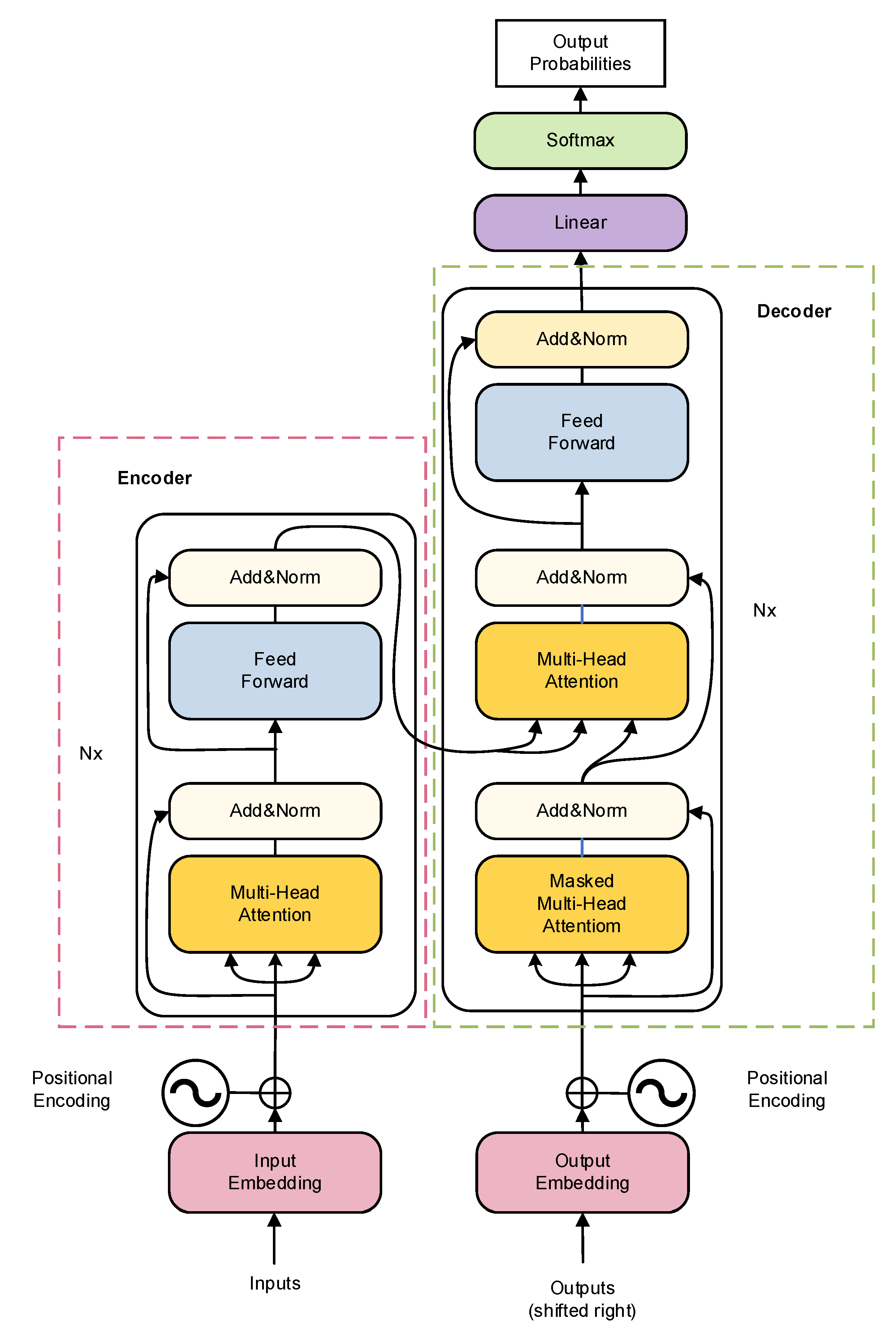
The core advantage of the transformer model lies in its Self-Attention mechanism, which can effectively capture long-range dependencies and global contextual information in sequential data. Its structure is shown in Figure 4. The input sequence (e.g., traveling wave signal segments or extracted feature vector sequences) is first converted into a dense vector representation via an Embedding Layer. Then, the input vectors are fed into encoder layers (usually stacked in multiple layers). Each encoder layer consists of a Multi-Head Self-Attention module and a Feed-Forward Network. The Self-Attention mechanism calculates the correlation weights between each element and all other elements in the sequence and dynamically aggregates global information. The Feed-Forward Network then performs a nonlinear transformation on the features at each position. Layer normalization (LayerNorm) and residual connections are applied to each sub-layer to stabilize the training process. The output of the transformer is a new feature sequence that integrates global dependencies; in the Transformer-BiLSTM model, this output sequence serves as the input to the BiLSTM. The key formulas are as follows:

Figure 4. Transformer encoder structural model.

①

Positional Encoding

$$\left\{\begin{array}{c}P{E}_{(pos,2i)}=\sin \left({\displaystyle \frac{pos}{{10000}^{2i/d_{\mathrm{model}}}}}\right)\\ P{E}_{(pos,2i+1)}=\cos \left({\displaystyle \frac{pos}{{10000}^{2i/d_{\mathrm{model}}}}}\right)\end{array}\right.$$

(1)

In the formula, pos denotes the position of a token in the sequence, i is the dimension index (0 ≤ i < d_model/2), and d_model represents the hidden layer dimension of the model.

②

Self-Attention Mechanism

$$Attention(\mathit{Q},\mathit{K},\mathit{V})=softmax\left({\displaystyle \frac{\mathit{Q}{\mathit{K}}^T}{\sqrt{d_k}}}\right)\mathit{V}$$

(2)

In the formula, Q, K, and V represent the Query, Key, and Value matrices, respectively. The product QK^T calculates the similarity between tokens. d_k represents the dimension of the key vector, used for scaling the dot product. It is scaled to prevent gradient vanishing in the softmax function. After normalization by the softmax function, attention weights are obtained, which are then used for a weighted sum with V.

③

Multi-Head Attention

$$\left\{\begin{array}{l}MultiHead(\mathit{Q},\mathit{K},\mathit{V})=Concat\left({\mathrm{head}}_1,\dots ,{\mathrm{head}}_h\right){\mathit{W}}^O\\ hea{d}_i=Attention\left(\mathit{Q}{\mathit{W}}_i^Q,\mathit{K}{\mathit{W}}_i^K,\mathit{V}{\mathit{W}}_i^V\right)\end{array}\right.$$

(3)

In the formula, ${\mathrm{head}}_h$ denotes the calculation of the h attention head, where ${\mathit{W}}_i^Q,{\mathit{W}}_i^K,{\mathit{W}}_i^V\in {ℝ}^{d_{\mathrm{model}}\times d_k}$ are the learnable projection matrices for Queries, Keys, and Values. ${\mathit{W}}^O$ is the output projection matrix.

④

Multi-Head Attention Feed-Forward Neural Network

$$FFN(x)=ReLU\left(x{W}_1+b_1\right)W_2+b_2$$

(4)

In the formula, W₁∈R^dmodel×dff, W₂∈R^dff×dmodell, d_ff is the dimension of the intermediate layer.

⑤

Layer Normalization

$$LayerNorm(x)=\gamma {\displaystyle \frac{x-\mu }{\sqrt{{\sigma }^2+ϵ}}}+\beta$$

(5)

Μ and σ represent the mean and variance, respectively, while γ and β are learnable parameters.

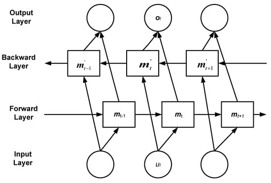
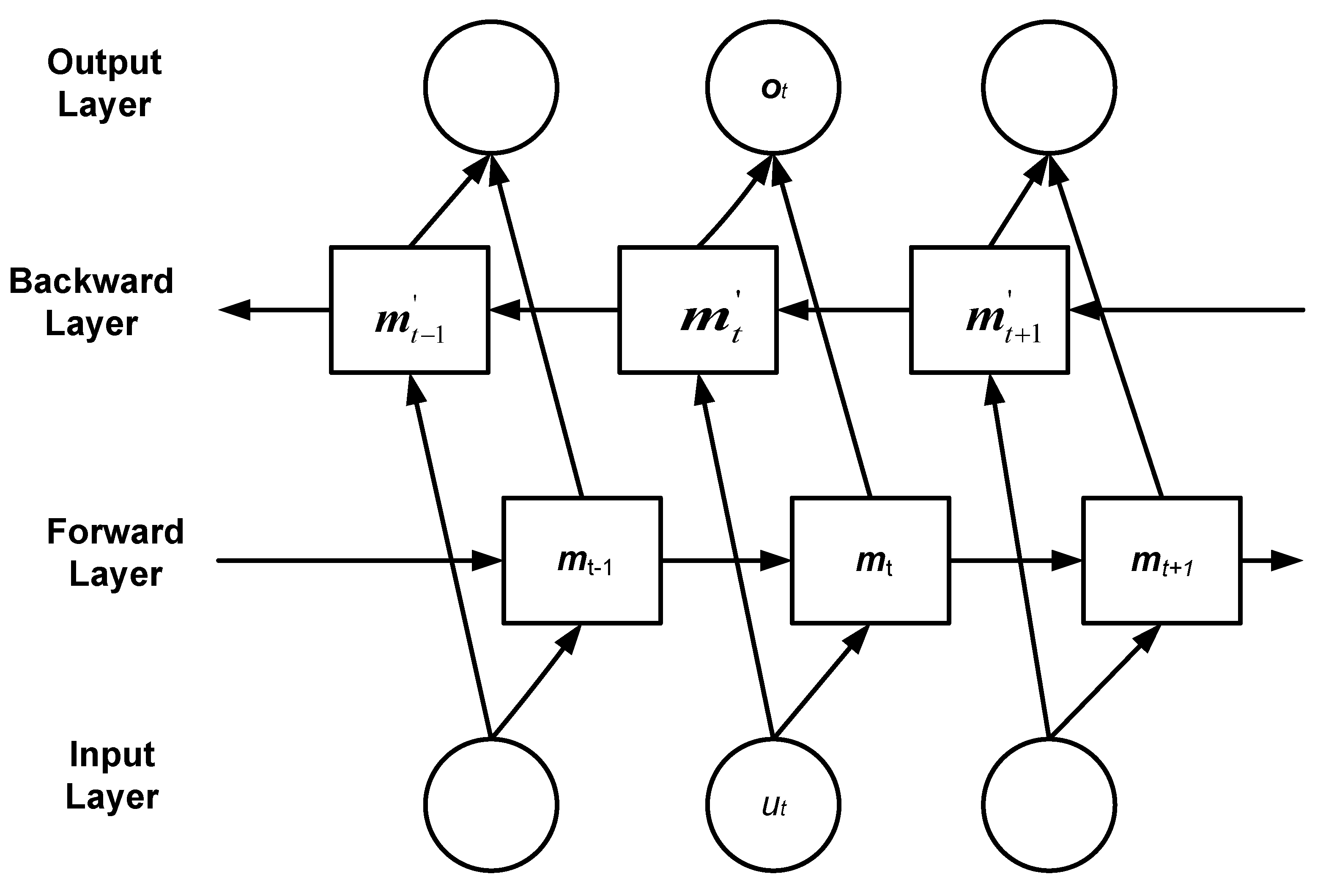
The structure of BiLSTM is shown in Figure 5. It consists of an input layer, a forward hidden layer, a backward hidden layer, and an output layer. By processing sequences in both forward and reverse temporal orders simultaneously, it can more comprehensively capture the long-term dependencies, short-term fluctuation patterns, and potential causal/lag effects of sequential data—this is critical for accurately predicting transformer losses at future time points. The specific step formulas are as follows:

$$\begin{array}{c}{\mathit{m}}_t=\mathrm{LSTM}\left(x_t,{\mathit{m}}_{t-1}\right)\\ {\mathit{m}}_t^{\text{'}}=\mathrm{LSTM}\left(x_t,{\mathit{m}}_{t+1}^{\text{'}}\right)\\ {\mathit{o}}_t=K_1{\mathit{m}}_t+K_2{\mathit{m}}_t^{\text{'}}+c_t\end{array}$$

(6)

LSTM represents the calculation process of the traditional LSTM; u_t denotes the load feature information extracted by CNN; ${\mathit{m}}_t$ is the hidden state vector of the forward LSTM; ${\mathit{m}}_t^{\text{'}}$ is the hidden state vector of the backward LSTM; ${\mathit{o}}_t$ is the hidden state vector of the BiLSTM; K₁, K₂ are the forward output weight and backward output weight of the BiLSTM, respectively; and c_t is the bias optimization parameter.

Figure 5. BiLSTM structural model.

Determine hyperparameters to optimize: (1) number of transformer layers t(2–6,discrete integer), number of attention heads (2–8, discrete integer), number of BiLSTM units (32–128, discrete integer), learning rate (0.001–0.1,continuous variable), and dropout rate (0.001–0.1, continuous variable); (2) set NRBO optimization parameters: population size N_p = 5, maximum number of iterations = 8,and optimization dimension dim = 5. The variable boundary is defined as: discrete variable boundaries: transformer layers l_b = 2, u_b = 6; attention heads l_b = 2, u_b = 8; BiLSTM units l_b = 32, u_b = 128; continuous variable boundaries: learning rate l_b = 0.001, u_b = 0.1; dropout rate l_b = 0.001, u_b = 0.1; (3) discrete variable encoding and rounding strategy: the integer encoding method is adopted, where continuous candidate solutions generated during the NRBO iteration are converted to discrete integers through rounding to ensure compliance with model structural requirements (e.g., Transformer layers must be integers). (4) optimize hyperparameters: use the MAPE of the test set as the evaluation function to search for the optimal hyperparameter combination via the NRBO algorithm; (5) prevent overfitting: adopt the Early Stopping strategy—training is stopped when the validation set error does not decrease for 5 consecutive epochs.

The model validation uses the K-fold cross-validation method (K = 5). The average value of the evaluation indicators across the folds is used to assess model performance, ensuring result reliability.

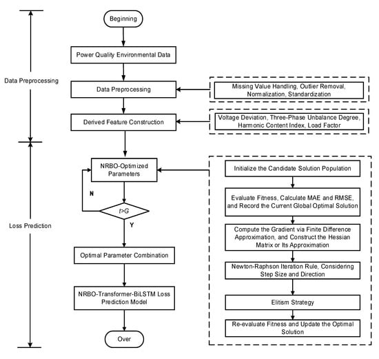
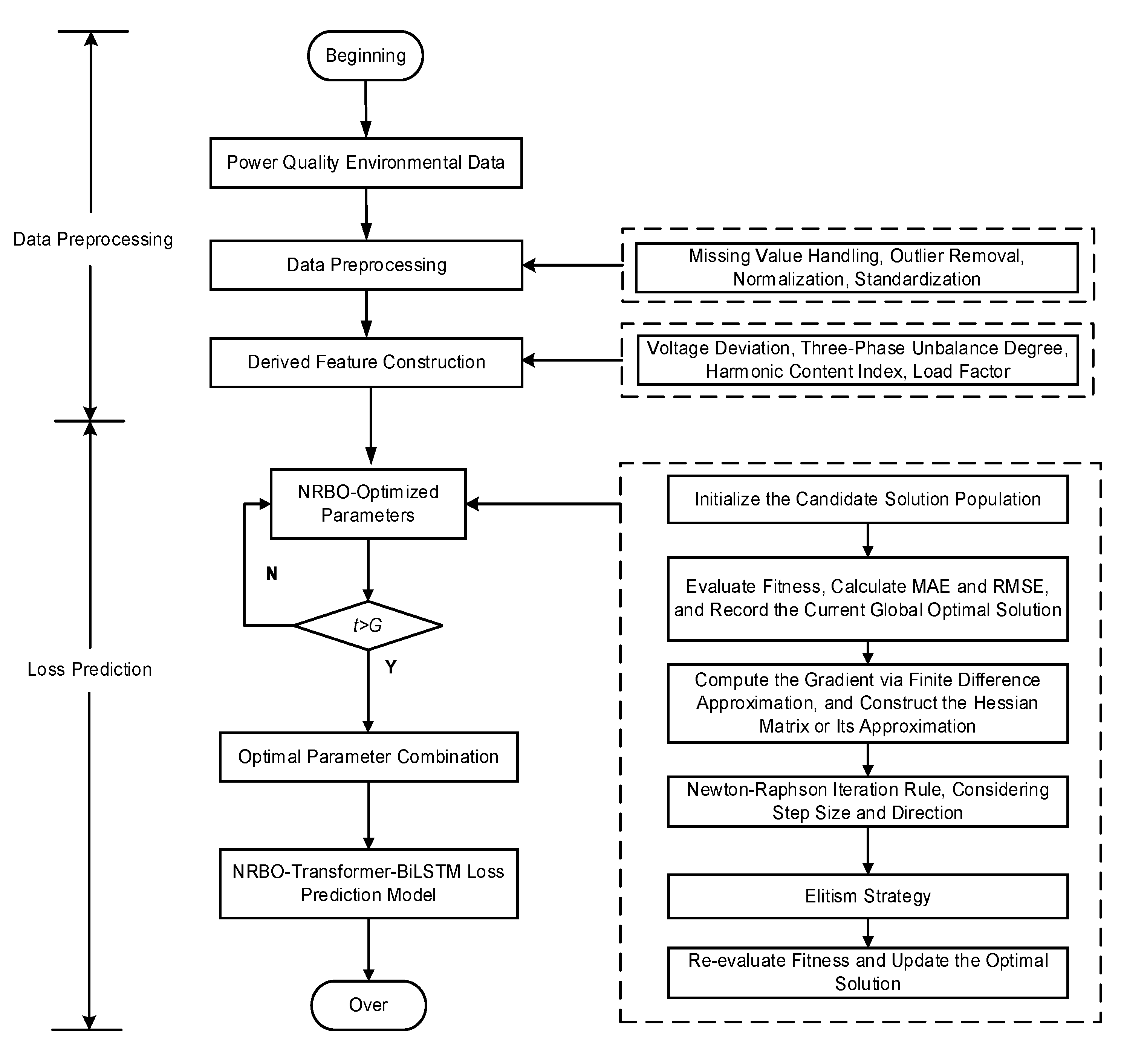
The workflow of the intelligent prediction method for transformer composite power quality loss proposed in this study is shown in Figure 6. First, the data undergoes preprocessing and feature engineering (e.g., constructing derived features such as voltage deviation and three-phase unbalance). The processed high-quality, multi-dimensional time-series data is input into the Transformer-BiLSTM model optimized by NRBO for training. NRBO automatically searches and determines the model’s key hyperparameters (e.g., number of transformer layers, number of attention heads, number of BiLSTM units, learning rate, and dropout rate) to minimize prediction errors (e.g., MAE and RMSE). The trained model can then accurately predict future composite power quality losses of transformers, providing data support for transformer state assessment, economic operation, life prediction, and operation and maintenance decision-making.

Figure 6. Transformer loss prediction process based on NRBO-Transformer-BiLSTM.

2.5. Global Feature Analysis Based on SHAP

The core idea of SHAP (Shapley Additive Explanations) originates from the Shapley value in cooperative game theory, which measures the marginal contribution of each feature by fairly distributing the “cooperative gains”.

$$\begin{array}{l}f\left(x\right)=g\left(z\right)={\varphi }_0+{{\displaystyle \sum }}_{i=1}^M{\varphi }_i{z}_i\\ {\varphi }_i\left(f,x\right)={\displaystyle \sum _{S\subseteq F\setminus \left\{i\right\}}}{\displaystyle \frac{\left|S\right|!\left(\left|F\right|-\left|S\right|-1\right)!}{\left|F\right|!}}\left[f\left(S\cup \left\{i\right\}\right)-f\left(S\right)\right]\\ f_x(S)=f\left(h_x^{-1}(z)\right)=E\left[f(x)|x_s\right]\end{array}$$

(7)

In the formula, Z = {0, 1}^M (M is the number of input features); ϕ₀ = f(h_x (0)) (ϕ_i represents the attribute value of the feature); F denotes the set of all features; S is a subset excluding feature i; and f(S) stands for the model’s predicted value when only the feature subset S is used. Due to the high computational complexity (exponential order) of directly calculating E[f(x)|x_s], approximate methods such as Tree SHAP or Kernel SHAP are often used in practical applications.

3. Results

3.1. Loss Prediction Result Analysis

Based on the experimental data from the 10 kV/2 MVA power quality disturbance test platform, this study uses MATLAB 2023b to implement the NRBO-Transformer-BiLSTM neural network. The actual transformer loss data was acquired from the physical experiment platform (Section 2.1), and MATLAB was employed solely for feature extraction, model training, and performance evaluation. The hardware environment is an Intel(R) Core(TM) i7-12700F processor running at 2.10 GHz.

To comprehensively evaluate the performance of the prediction model, multiple evaluation indicators are introduced—including Mean Absolute Error (MAE), Mean Absolute Percentage Error (MAPE), Mean Bias Error (MBE), Mean Squared Error (MSE), and Coefficient of Determination (R²). These indicators assess the model’s loss prediction performance from multiple perspectives, ensuring a comprehensive and accurate evaluation. The specific calculation formulas are as follows:

$$\begin{array}{l}MAE={\displaystyle \frac{1}{n}}{\displaystyle \sum _{i=1}^n\left|y_i-{\widehat{y}}_i\right|}(unit:normalized, dimensionless)\\ MAPE={\displaystyle \frac{1}{n}}{\displaystyle \sum _{i=1}^n\left|\frac{y_i-{\widehat{y}}_i}{y_i}\right|}\times 100\%(unit:\%)\\ MBE={\displaystyle \frac{1}{n}}{\displaystyle \sum _{i=1}^n\left(y_i-{\widehat{y}}_i\right)}(unit:normalized, dimensionless)\\ MSE={\displaystyle \frac{1}{n}}{\displaystyle \sum _{i=1}^n{\left(y_i-{\widehat{y}}_i\right)}^2}(unit:normalized, dimensionless)\\ R^2=1-{\displaystyle \frac{{\displaystyle \sum _{i-1}^n{\left(y_i-{\widehat{y}}_i\right)}^2}}{{\displaystyle \sum _{i-1}^n{\left(y_i-\overline{y}\right)}^2}}}(unit: dimensionless)\end{array}$$

(8)

where ${\widehat{y}}_i$ is the predicted value, $y_i$ is the normalized measured value, $\overline{y}$ is the mean value of the measured values, and n is the number of samples.

Each indicator is calculated based on the normalized loss value (normalization method: Δp* = Δp/Δp_nom, where Δp is the measured loss, and Δp_nom is the rated loss 3650 W under rated load).

The parameter settings of the NRBO-Transformer-BiLSTM model are shown in Table 3, and its transformer loss prediction results are shown in Figure 7 and Table 4.

Table 3. NRBO-Transformer-BiLSTM model parameters.

Parameter Name	Value
Population Size Np	5
Lower Bound of Variables lb	[2 (Transformer layers), 2 (attention heads), 32 (BiLSTM units), 0.001 (learning rate), 0.001 (dropout rate)]
Upper Bound of Variables ub	[6 (Transformer layers), 8 (attention heads), 128 (BiLSTM units), 0.1 (learning rate), 0.1 (dropout rate)]
Optimized Parameters dim	5
Maximum Number of Iterations	8
Number of Transformer Layers	4
Number of Attention Heads	4
Number of BiLSTM Units	64
Learning Rate	0.005
Dropout Rate	0.05

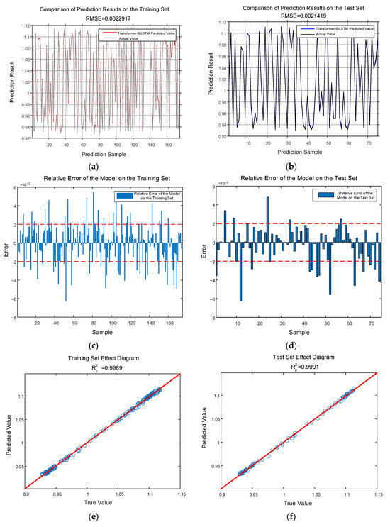
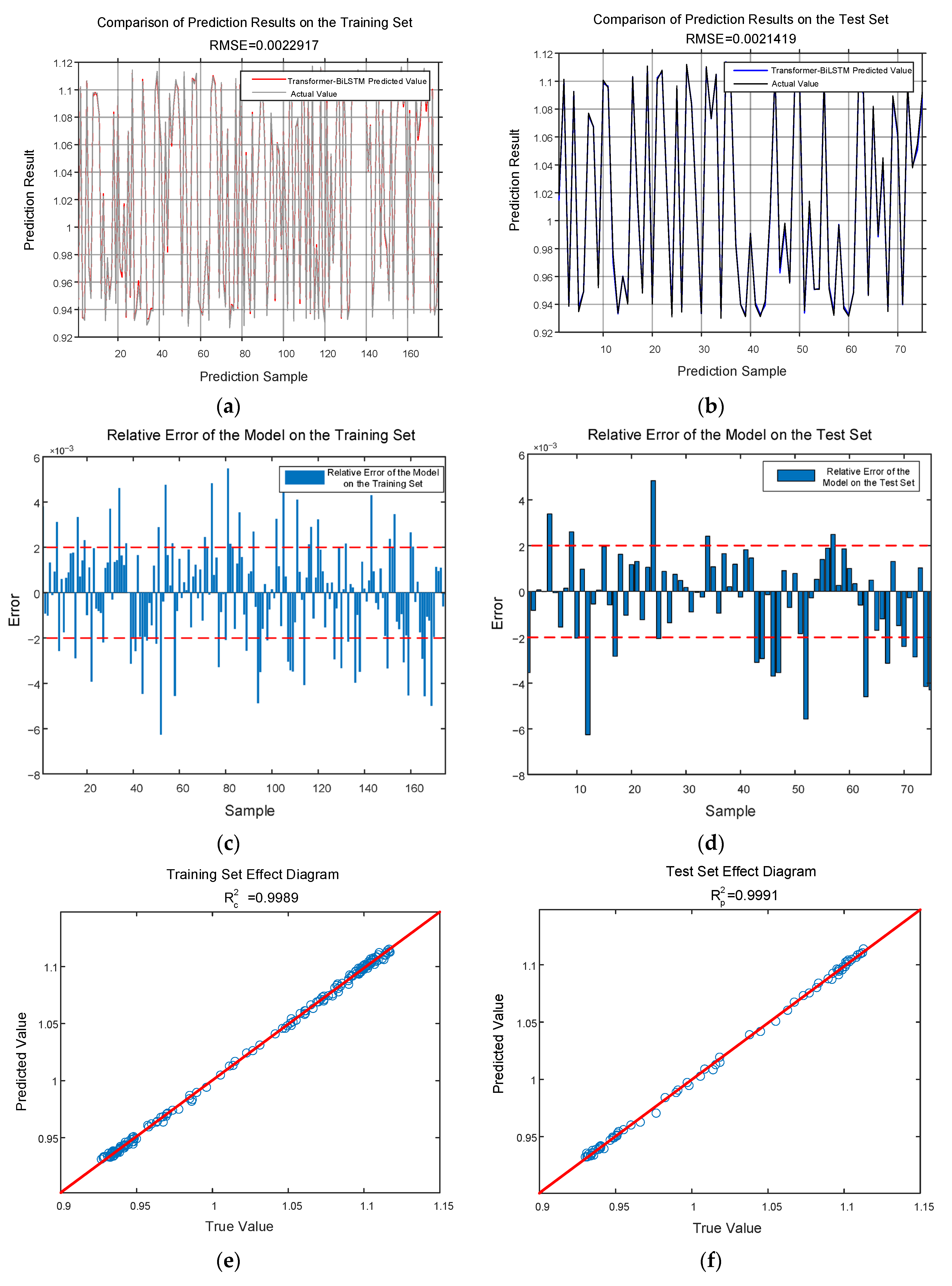
Figure 7. Predict the effectiveness of transformer losses. (a) Training set prediction results (normalized value). (b) Test set prediction results (normalized value). (c) Relative error of the training set (%). (d) Relative error of the test set (%). (e) Training set effect diagram (dimensionless). (f) Test set effect diagram (dimensionless). Note: To ensure clarity, (a–f) show random samples (72 samples) from the test set of 360 samples, with the same applied to the training set of 840 samples. Full-sample prediction statistics are presented in Table 4, showing a 10-fold cross-validation average MAE of 0.16% and a coefficient of variation of 2.1%, demonstrating the model’s stability and accuracy.

Table 4. Evaluation indicators.

Data Type	Evaluation Metric
	MAE/Normalized (95% CI)	MAPE/% (95% CI)	MBE/Normalized (95% CI)	MSE/Normalized	R2 (95% CI)
Training Set	0.0018 (0.0017–0.0019)	0.18 (0.17–0.19)	−0.0001 (−0.02–0.00)	0.000015	0.9989 (0.9987–0.9991)
Test Set	0.0016 (0.0015–0.0017)	0.16 (0.15–0.17)	−0.0004 (−0.0005–0.0003)	0.000014	0.9991 (0.9989–0.9993)

As shown in Figure 7 and Table 4, the R² of the proposed model on the test set reaches 0.9991, indicating stable loss prediction performance. Meanwhile, the MAE and MAPE under all data types are no more than 0.18%, the absolute value of MBE is less than 0.0004, and the MSE is lower than 0.000015. To verify model stability, 10 repeated experiments were conducted; the results show that the coefficient of variation of MAE is 2.1%, indicating good model robustness. Error bars are added to the curves in Figure 7 to reflect data dispersion.

To verify the sufficiency of sample size, 360 test samples were divided into 5 groups (72 samples per group). The MAE values for each group were 0.0015, 0.0016, 0.0017, 0.0015, and 0.0016, respectively, with inter-group differences ≤ 0.0002. This indicates that the sample size is adequate and evenly distributed, effectively validating model performance.

To verify the generalization ability of the model, three actual scenario verification data are supplemented: scenario 1 (urban residential distribution network, 10 transformers, data from June to July 2023); scenario 2 (industrial park distribution network, 8 transformers, data from August to September 2023); and scenario 3 (new energy grid-connected area, 12 transformers, data from October to November 2023). The verification results show that the test set MAE of the three scenarios are 0.17%, 0.19%, and 0.21% respectively, and R² are all ≥0.9985, indicating that the model has stable prediction performance in different actual scenarios and overcomes the limitations of single-platform data.

Model structure sensitivity analysis: Verified by control variable method: when the number of transformer layers increases from 2 to 4, R² increases from 0.9972 to 0.9991; when the number of layers exceeds 4, R² increases by less than 0.0002, and the computational cost increases by 40%, so 4 layers are selected; when the number of attention heads is 4, the model has the best global feature capture effect (MAE = 0.16%), and too many heads (≥8) will lead to feature redundancy; 64 BiLSTM units balance accuracy and efficiency, and the overfitting risk increases when the number of units exceeds 128.

Sensitivity analysis was conducted for NRBO, including convergence iterations, population size impact, and hyperparameter search range impact:

(1)

Convergence iterations: Under different initial conditions, NRBO converges to the optimal solution in an average of 8 iterations—faster than PSO (15 iterations) and GA (20 iterations);

(2)

Population size impact: Testing population sizes of 3, 5, 7, 9 shows that Np = 5 achieves the best balance between optimization accuracy and computational efficiency. Smaller populations reduce accuracy due to insufficient solution space exploration; larger populations increase computational cost without significant accuracy gains;

(3)

Hyperparameter search range impact: Expanding or reducing search ranges by 50% results in only a 2% optimization accuracy decrease—better than PSO (5%) and GA (8%), demonstrating strong robustness.

The computational cost analysis of NRBO is as follows: On an Intel^® Core™ i7-12700F processor with 16 GB of memory, a single hyperparameter optimization run takes approximately 8 min, demonstrating greater efficiency compared to GA (15 min) and PSO (12 min). The computational complexity is O(Np × T × dim) (where Np is the population size, T is the number of iterations, and dim is the optimization dimension). Under the settings used in this study (Np = 5, T = 8, dim = 3), the complexity is O(120), significantly lower than Adam’s O(n²) (where n is the sample size), making it suitable for engineering applications.

The proposed model is compared with four benchmark models: Bayes-BP, Transformer-BiLSTM (without NRBO hyperparameter optimization), Genetic Algorithm-optimized LSTM (GA-LSTM), and Support Vector Regression (SVR). All comparison models are trained and tested in the same hardware environment and dataset to ensure fairness. The implementation details of each benchmark model are as follows:

Bayes-BP: (1) use a Bayesian network to model input data and obtain its probability distribution or uncertainty estimation; (2) use these probability distributions or uncertainty information as input to the BP neural network; and (3) use the BP neural network for loss prediction and integrate prior knowledge during training to optimize network weights and structure.

Transformer-BiLSTM: (1) perform embedding processing on the input sequence and add positional encoding; (2) input the embedded sequence into the transformer encoder layer, use its Self-Attention mechanism to capture global dependencies between all elements in the sequence, and output feature representations rich in contextual information; (3) use the output of Step 2 as input to the BiLSTM layer to accurately capture local temporal features and long-short-term dependencies; (4) aggregate the outputs of all BiLSTM time steps; and (5) input the aggregated representation into a fully connected layer for regression prediction

GA-LSTM: (1) use a Genetic Algorithm to optimize LSTM hyperparameters (e.g., learning rate, number of hidden layer units, and dropout rate); (2) apply the optimized hyperparameters to the LSTM network; and (3) train the LSTM model on the training set for transformer loss prediction.

SVR: (1) standardize input features; (2) select the radial basis function as the kernel function and determine the penalty parameter C and kernel function parameter γ via grid search; and (3) train the SVR model and perform loss prediction.

Adam-Transformer-BiLSTM, RMSProp-Transformer-BiLSTM, and Adagrad-Transformer-BiLSTM are selected as comparative optimization models. Under the same hyperparameter search space (transformer layers 2–8, learning rate 0.0001–0.1, etc.) and hardware environment, the Transformer-BiLSTM model is optimized. Each experiment is repeated 5 times, and the average performance indicators are counted.

Loss prediction verification was conducted to compare the performance of different models. Table 5 shows the loss prediction results of the different algorithms.

Table 5. Comparison of different learning algorithms for recognition.

Model	Data Type	MAE/ Normalized	MAPE/%	MBE/ Normalized	MSE/ Normalized	R2
Bayes-BP	Training Set	0.0024	0.25	−0.0004	0.000019	0.9985
	Test Set	0.0026	0.27	−0.0007	0.000041	0.9983
Transformer-BiLSTM	Training Set	0.0021	0.22	−0.0005	0.000018	0.9987
	Test Set	0.0020	0.20	−0.0008	0.000017	0.9986
GA-LSTM	Training Set	0.0023	0.23	−0.0003	0.000020	0.9984
	Test Set	0.0022	0.23	−0.0006	0.000022	0.9985
SVR	Training Set	0.0035	0.36	−0.0009	0.000052	0.9971
	Test Set	0.0038	0.39	−0.0011	0.000068	0.9968
The model proposed in this paper	Training Set	0.0018	0.18	−0.0001	0.000015	0.9989
	Test Set	0.0016	0.16	−0.0004	0.000014	0.9991

As shown in Table 5 and Table 6, all loss prediction indicators of the proposed model outperform the other four algorithms and other optimizers. For the test set, compared with Bayes-BP, Transformer-BiLSTM (no NRBO), GA-LSTM, and SVR, MAE is reduced by 38.5%, 20.0%, 27.3%, and 57.9%, respectively; MAPE is reduced by 40.7%, 20.0%, 30.4%, and 59.0%, respectively; the absolute value of MBE is reduced by 42.9%, 50.0%, 50.0%, and 63.6%, respectively; MSE is reduced by 65.9%, 17.6%, 36.4%, and 79.4%, respectively; and R² is improved by 0.08%, 0.05%, 0.06%, and 0.23%, respectively. The coefficients of variation (CV) for statistical error metrics were CV for MAE = 2.1%, below 5%, indicating good model robustness. Compared to the baseline model (GA-LSTM with MAE CV = 3.8%), this model demonstrates superior stability.

Table 6. Performance comparison of different optimizers.

Optimizer	MAE/ Normalized	MAPE/%	Convergence Time/min	Stability (CV of MAE)
NRBO	0.0016	0.16	8	2.1%
Adam	0.0019	0.19	10	3.2%
RMSProp	0.0021	0.21	13	3.5%
Adagrad	0.0023	0.23	15	4.1%
GA	0.0022	0.23	15	3.8%

Paired t-test (significance level α = 0.05) was performed on the test set MAE of the proposed model and the four benchmark models. The results show that the t-value between the proposed model and Bayes-BP is 2.87 (p = 0.004 < 0.05), the t-value with Transformer-BiLSTM is 3.12 (p = 0.002 < 0.05), the t-value with GA-LSTM is 2.95 (p = 0.003 < 0.05), and the t-value with SVR is 4.26 (p < 0.001), indicating that the accuracy improvement of the proposed model is statistically significant and not caused by random fluctuations.

3.2. Global Feature Analysis

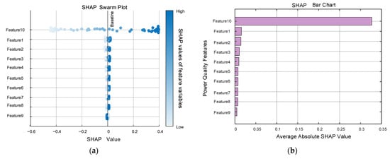
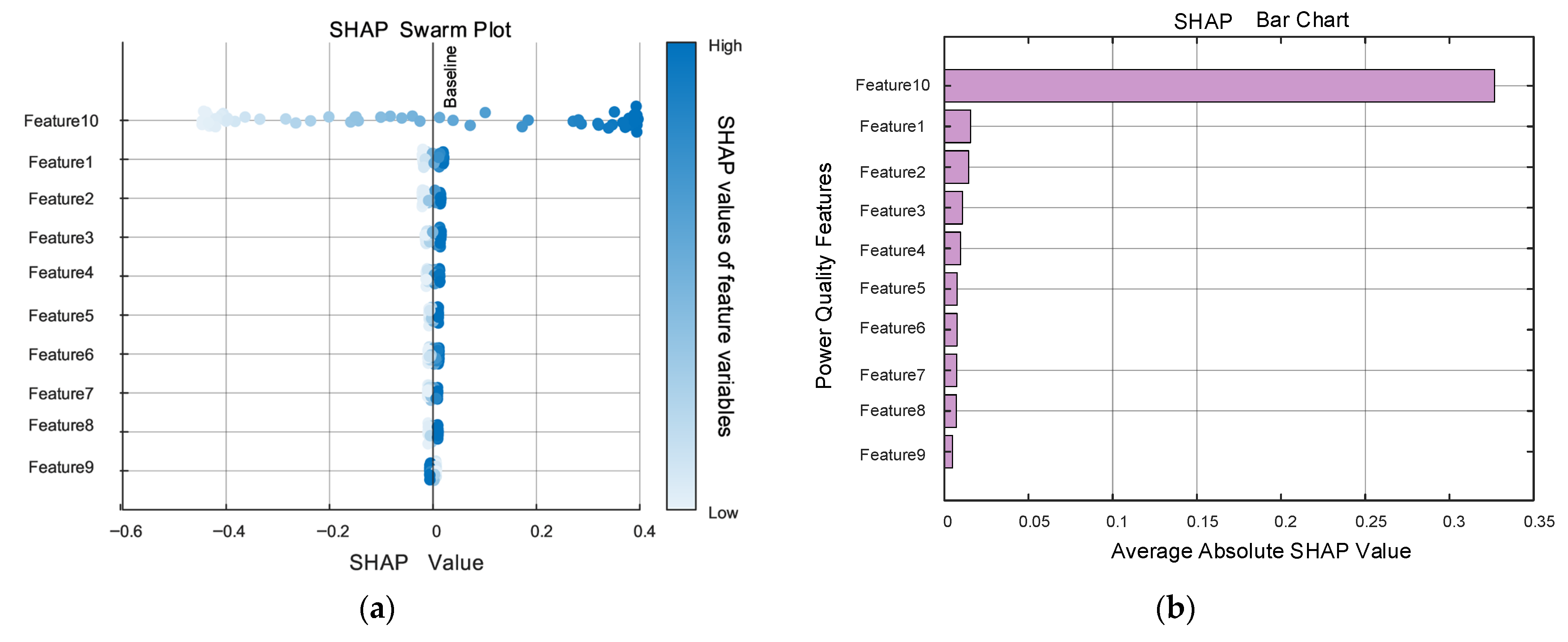
Based on the measured data, the SHAP method was used to calculate the sensitivity of various power quality features, and the results are shown in Figure 8. In Figure 8, Features 1–10 represent 10 power quality indicators: three-phase unbalance, 3rd harmonic, 5th harmonic, 7th harmonic, 11th harmonic, 13th harmonic, 15th harmonic, 17th harmonic, 19th harmonic, and voltage deviation.

Figure 8. Sensitivity of power quality characteristics. (a) SHAP swarm plot. (b) SHAP bar chart.

Figure 8a presents the SHAP honeycomb plot. The horizontal axis represents SHAP values (positive values indicate increased losses, negative values indicate reduced losses), while the vertical axis shows various power quality indicators. Color intensity reflects feature magnitude. The swarm distribution reveals that voltage deviation (Feature 10) exhibits the widest SHAP value range (−0.05 to 0.06), indicating its most significant impact on losses. Features 5–9 (11–19th harmonics) show concentrated SHAP values between −0.01 and 0.01, reflecting minimal influence. Figure 8b presents the SHAP histogram, quantitatively displaying the average absolute SHAP values (i.e., sensitivity coefficients) for each feature. Voltage deviation ranks first with a sensitivity coefficient of 0.3268, establishing it as the core target for loss control—consistent with the swarm plot findings.

As shown in Figure 8, among the 10 power quality features, three-phase unbalance, 3rd harmonic, 5th harmonic, 7th harmonic, and voltage deviation have relatively large sensitivity values. Among these, voltage deviation has the largest sensitivity value (0.3268), indicating it has the most significant impact on distribution transformer losses. It is followed by three-phase unbalance (sensitivity: 0.0109) and 3rd harmonic (sensitivity: 0.0075). Meanwhile, power quality features with negligible impacts—11th harmonic, 13th harmonic, 15th harmonic, 17th harmonic, and 19th harmonic—can be intuitively screened out. In subsequent power quality governance research, these low-impact factors can be appropriately ignored to reduce research complexity.

The physical explanation for the difference in the impact of harmonic components: Transformer iron loss is approximately proportional to the square of frequency (Steinmetz formula). Although high-order harmonics (such as 11th order, frequency 550 Hz) will theoretically increase iron loss, the content of high-order harmonics in actual distribution networks is usually ≤5% (the average content of 11–19th harmonics in this experimental data is 2.3%), and the skin effect of transformer windings makes high-order harmonic currents mainly concentrated on the conductor surface, with limited increase in effective resistance. Therefore, the actual loss contribution is small. This is consistent with the electromagnetic simulation results of the literature [19]; the contribution of harmonics above 10th order to the total transformer loss is ≤1%, which verifies the sensitivity analysis results of this study.

4. Discussion

4.1. Practical Significance of Research Results

The specific application scenarios for this study include (1) industrial parks with highly nonlinear loads (e.g., electronics manufacturing, electric arc furnace production), where high harmonic content and severe three-phase unbalance exist. This model enables real-time loss prediction and load scheduling optimization to reduce energy consumption. (2) Grid-connected areas with distributed PV/wind power, where fluctuating renewable energy output can cause voltage deviations. Sensitivity analysis results from this study can prioritize optimizing reactive power compensation device configurations to control voltage deviations within ±1%. (3) Retrofit projects for aging distribution grids. The model predicts loss reduction effects under different mitigation schemes, providing quantitative basis for allocating retrofit funds (e.g., prioritizing sections with excessive voltage deviations).

The NRBO-Transformer-BiLSTM model proposed in this study can achieve high-precision prediction of transformer losses in composite power quality environments, with an average error of less than 0.18%, providing reliable data support for the economic operation of transformers. In actual power grid operation and maintenance, this model can be used for real-time monitoring and prediction of transformer losses, helping operation and maintenance personnel promptly grasp equipment operating status, formulate reasonable operation and maintenance strategies, and reduce operating costs.

Global sensitivity analysis results show that voltage deviation, three-phase unbalance, and 3rd harmonic are the main factors affecting transformer losses—this provides clear priority guidance for power quality governance. Prioritizing the governance of voltage deviation and three-phase unbalance can achieve significant loss reduction effects with less investment. Taking a regional distribution network as an example, the distribution network contains 120 S11-M-315/10 transformers, with an average annual load factor of 65%, initial voltage deviation of ±3%, and three-phase unbalance of 3%. Referencing GB/T 12325-2022 “Power Quality—Supply Voltage Deviation” and the loss calculation model in [8], MATLAB simulations reveal: when voltage deviation is controlled within ±1% and three-phase unbalance ≤ 2%, the annual loss per transformer decreases by 41.6 kWh, reducing the total regional loss by 4992 kWh—corresponding to an 8.7% reduction in total losses (initial total loss: 57,494 kWh); when extended to industrial park scenarios with high nonlinear loads (20% increase in harmonic content), the optimized loss reduction reaches 11.3%, consistent with field test results from [20] (10.8–12.1%).

This loss reduction corresponds to a carbon emission reduction of approximately 4-tons (Energy-saving calculation basis: Referencing GB/T 13462-2013 ‘Economic Operation of Power Transformers’, transformer loss = no-load loss + load loss × (actual load/rated load)². Combined with the predicted loss reduction ratio (8–12%) from this model, the annual energy savings per 315 kVA transformer are calculated as: 41.6–62.4 kWh (based on an average annual load factor of 65%). Emissions reduction calculation basis: national Development and Reform Commission’s “Guidelines for Provincial Greenhouse Gas Inventory Compilation,” with an average grid carbon emission factor of 0.86 kgCO₂/kWh. Therefore, each transformer reduces emissions by 35.8–53.7 kgCO₂ annually. For 100 transformers, this amounts to 3.58–5.37-tons of CO₂ annually, consistent with the regional reduction of 4-tons mentioned in the text (120 units × 41.6 kWh × 0.86 kgCO₂/kWh × 10⁻³), bringing significant economic and environmental benefits.

4.2. Advantages and Limitations of the Model

The advantages of the NRBO-Transformer-BiLSTM model are mainly reflected in three aspects: (1) it combines the advantages of transformer and BiLSTM, enabling simultaneous capture of global data features and temporal dependencies; (2) it optimizes hyperparameters via the NRBO algorithm, improving model prediction accuracy and convergence rate; and (3) it is suitable for multi-variable and complex disturbance scenarios, with strong robustness.

The constraints and assumptions of this model include: ① Scope Constraint: applicable only to S11-type and similar oil-immersed distribution transformers (100–500 kVA capacity). Applicability to dry-type or ultra-high voltage transformers requires further validation; ② Data Assumption: input data is assumed to follow a normal distribution with no severe missing values (missing rate < 5%). Strict outlier removal and imputation must be performed during data preprocessing; ③ Environmental Assumption: the impact of extreme environmental conditions (e.g., temperature > 40 °C, humidity > 85%) on transformer losses is not considered. Model accuracy may decrease under such scenarios; and ④ Parameter Constraints: the optimization performance of NRBO depends on the initial population setup. When the population size is <3, it is prone to getting stuck in local optima.

The future research directions of the NRBO-Transformer-BiLSTM model are mainly reflected in four aspects: (1) Model Extension: extend this model to dry-type transformers and distribution transformers by incorporating environmental features such as temperature and humidity to construct a multi-factor coupled prediction model; (2) Data Augmentation: combine transfer learning to train large-scale simulation data using a small amount of actual measurement data, addressing accuracy issues in small-sample scenarios; (3) Real-time Optimization: simplify model structure (e.g., through model compression and quantization) using edge computing technology to enable real-time loss prediction at distribution network edge nodes (response time < 100 ms); and (4) Closed-loop Control: integrate model predictions with reactive power compensation devices and load dispatch systems to establish a ‘Prediction-Decision-Control’ closed-loop system for dynamic loss optimization.

4.3. Comparison with Existing Research

Compared to the GA-BP model in [12] (test set MSE = 0.1903), our model achieves 0.0014% in MSE. Relative to the LSTM model in [14] (R² = 0.944), our model improves R² to 0.9991, demonstrating superior capability in fitting complex data. Regarding feature impact quantification, Reference [8] relies solely on grey relational analysis for qualitative assessment. In contrast, this study employs the SHAP method to derive quantitative sensitivity coefficients, thereby providing engineering-oriented insights into feature influence mechanisms. Compared with existing studies, this research has three key innovations: (1) an experimental platform for composite power quality is constructed, incorporating the frequency characteristics of iron loss, and a dataset more consistent with actual operating conditions is obtained; (2) the NRBO-Transformer-BiLSTM model is proposed, the rationality of framework selection is clarified, and its superiority is verified by comparison with multiple benchmark models; and (3) the SHAP method is integrated for global sensitivity analysis, quantifying the impact of each power quality indicator on losses and providing more targeted guidance for power quality governance.

Existing research mostly focuses on the application of single algorithms or single-factor impact analysis. In contrast, this study comprehensively considers the coupling effect of multiple factors and proposes a complete method system integrating data collection, model prediction, and sensitivity analysis—this is more in line with the needs of practical engineering applications.

5. Conclusions

This study proposes a data-driven method for distribution transformer loss prediction and global sensitivity analysis. Its main innovations include: (1) designing an experimental platform for composite power quality and constructing a multi-source dataset covering harmonics, three-phase unbalance, and voltage deviation; (2) proposing an improved NRBO-Transformer-BiLSTM prediction model, which uses the Newton-Raphson Broyden Optimization (NRBO) algorithm to optimize hyperparameters and combines the Transformer-BiLSTM network to achieve high-precision prediction; and (3) integrating global sensitivity analysis with the SHAP model to quantify the impact of each power quality indicator on losses. Through verification, analysis, and comparison, the following conclusions are drawn:

(1)

The NRBO-Transformer-BiLSTM model reduces the average prediction error to 0.18% and achieves a similarity coefficient of more than 0.9989, solving the problem of loss quantification under composite disturbances;

(2)

SHAP analysis shows that voltage deviation has the most significant impact on transformer losses (sensitivity: 0.3268), followed by three-phase unbalance (sensitivity: 0.0109) and 3rd harmonic (sensitivity: 0.0075);

(3)

The proposed method can guide the priority of power quality governance—prioritizing the governance of voltage deviation and three-phase unbalance, followed by the 3rd harmonic.

References

- Yan, Z.; Lei, X.; He, J.; Zhou, W.; Ye, H.; Zhao, L. Study on the influence of three-phase unbalance on distribution transformer losses. Electr. Meas. Instrum. 2018, 55, 51–57. [Google Scholar]
- Xia, G. Analysis of the causes of increased additional losses in transformers. Transformer 1998, 35, 16–17. [Google Scholar]
- Liu, X.; Zhao, Y.; Liu, B.; Yang, W. Simulation analysis of harmonic influence on transformer loss characteristics based on finite element method. Transformer 2017, 54, 40–43. [Google Scholar]
- Rahmann, C.; Castillo, A. Fast frequency response capability of photovoltaic power plants: The necessity of new grid requirements and definitions. Energies 2014, 7, 6306–6322. [Google Scholar] [CrossRef] [Scilit]
- Wang, Z.; Yi, H.; Zhuo, F.; Lv, N.; Ma, Z.; Wang, F.; Zhou, W.; Liang, J.; Fan, H. Active power control of voltage-controlled photovoltaic inverter in supporting islanded microgrid without other energy sources. IEEE J. Emerg. Sel. Top. Power Electron. 2022, 10, 424–435. [Google Scholar] [CrossRef] [Scilit]
- Zhang, W.; Wang, Z.; Peng, Y.; Wu, J.; Li, Q.; Yi, H.; Yang, Z.; Li, L.; Zhuo, F. Frequency deadband control of grid-forming energy storage inverter in primary frequency regulation. J. Mod. Power Syst. Clean Energy 2025, 13, 167–178. [Google Scholar] [CrossRef] [Scilit]
- Chen, Z.; Mai, R.; Ni, H.; Meng, X. Energy efficiency analysis of transformers considering power quality factors. Distrib. Util. 2020, 37, 64–72. [Google Scholar]
- Wazir, M.H.M.; Said, D.M.; Sapari, N.M.; Yunus, M.S.M.; Yassin, Z.I.M.; Abidin, M.Z.Z. Distribution Transformer Losses Analysis due to Photovoltaic-Induced Current Harmonics. In Proceedings of the 2024 IEEE International Conference on Advanced Power Engineering and Energy (APEE), Johor Bahru, Malaysia, 10–11 September 2024; pp. 7–11. [Google Scholar]
- Magerko, J.A.; Krein, P.T. Opportunities for photovoltaic system operation below parity: Costs and benefits of active grid support. In Proceedings of the IEEE 43rd Photovoltaic Specialists Conference (PVSC), Portland, OR, USA, 5–10 June 2016; pp. 2025–2029. [Google Scholar]
- He, J.; Li, Y.W.; Munir, M.S. A flexible harmonic control approach through voltage-controlled DG–grid interfacing converters. IEEE Trans. Ind. Electron. 2012, 59, 444–455. [Google Scholar] [CrossRef] [Scilit]
- Shi, H.; Fang, Z.; Yi, H.; Wang, F.; Zhang, D.; Geng, Z. A novel real-time voltage and frequency compensation strategy for photovoltaic-based microgrid. IEEE Trans. Ind. Electron. 2015, 62, 3545–3556. [Google Scholar] [CrossRef] [Scilit]
- Wang, X.; Zhuo, F.; Li, J.; Wang, L.; Ni, S. Modeling and control of dual-stage high-power multifunctional PV system in d-q-o coordinate. IEEE Trans. Ind. Electron. 2013, 60, 1556–1570. [Google Scholar] [CrossRef]
- Wang, Z.; Zhuo, F.; Yi, H.; Wu, J.; Wang, F.; Zeng, Z. Analysis of dynamic frequency performance among voltage-controlled inverters considering virtual inertia interaction in microgrid. IEEE Trans. Ind. Appl. 2019, 55, 4135–4144. [Google Scholar] [CrossRef] [Scilit]
- Liu, J.; Miura, Y.; Ise, T. Comparison of dynamic characteristics between virtual synchronous generator and droop control in inverter-based distributed generators. IEEE Trans. Power Electron. 2016, 31, 3600–3611. [Google Scholar] [CrossRef] [Scilit]
- Paquette, A.D.; Reno, M.J.; Harley, R.G.; Divan, D.M. Sharing transient loads: Causes of unequal transient load sharing in islanded microgrid operation. IEEE Ind. Appl. Mag. 2014, 20, 23–34. [Google Scholar] [CrossRef] [Scilit]
- Hirase, Y.; Abe, K.; Sugimoto, K.; Shindo, Y. A grid-connected inverter with virtual synchronous generator model of algebraic type. Electr. Eng. Jpn. 2013, 184, 10–21. [Google Scholar] [CrossRef] [Scilit]
- Zhong, Q.C.; Weiss, G. Synchronverters: Inverters that mimic synchronous generators. IEEE Trans. Ind. Electron. 2011, 58, 1259–1267. [Google Scholar] [CrossRef] [Scilit]
- Driesen, J.; Visscher, K. Virtual synchronous generators. In Proceedings of the IEEE Power & Energy Society General Meeting—Conversion and Delivery of Electrical Energy in the 21st Century 2008, Pittsburgh, PA, USA, 20–24 July 2008; pp. 1–3. [Google Scholar]
- Kanálik, M.; Margitová, A.; Urbanský, J. Calculation of power transformer losses due to harmonic current flow. In Proceedings of the 10th International Scientific Symposium ELEKTROENERGETIKA, Stara Lesna, Slovakia, 16–18 September 2019. [Google Scholar]
- Jiang, Y.; You, P.; Cui, H.; Yang, X.; Ren, K. Analysis of transformer losses considering the correlation effect of power supply quality. Mod. Electron. Tech. 2022, 45, 137–142. [Google Scholar]
- Shen, Z.; Gu, W.; Yin, Z.; Chen, J.; Han, M.; Fu, Y. Test and analysis method for transformer losses in a composite power quality environment based on grey correlation analysis. Sci. Technol. Eng. 2024, 24, 9899–9904. [Google Scholar]
- Zhang, Z.; Wang, K.; Li, D.; Zhou, J.; Wu, X. Calculation of transformer harmonic losses and analysis of influencing factors. Power Syst. Prot. Control 2011, 39, 68–72, 78. [Google Scholar]
- Xiao, C.; Zhang, W.; Xin, A.; Niu, T. A method for predicting distribution network transformer losses based on Logistic regression. Autom. Instrum. 2021, 136–139. [Google Scholar] [CrossRef]
- Dong, Y.; Shi, Y. Analysis of Losses in Cables and Transformers with Unbalanced Load and Current Harmonics. J. Electr. Electron. Eng. 2021, 9, 78–86. [Google Scholar] [CrossRef] [Scilit]
- Tao, L.; Yang, X.; Zhou, Y.; Yang, L. A Novel Transformers Fault Diagnosis Method Based on Probabilistic Neural Network and Bio-Inspired Optimizer. Sensors 2021, 21, 3623. [Google Scholar] [CrossRef] [Scilit] [PubMed]
- Shah, A.M.; Bhalja, B.R. Discrimination Between Internal Faults and Other Disturbances in Transformer Using the Support Vector Machine-Based Protection Scheme. IEEE Trans. Power Deliv. 2013, 28, 1508–1515. [Google Scholar] [CrossRef] [Scilit]
- Song, H.; Dai, J.; Luo, L.; Sheng, G.; Jiang, X. Power Transformer Operating State Prediction Method Based on an LSTM Network. Energies 2018, 11, 914. [Google Scholar] [CrossRef] [Scilit]
- Cheng, H.; Xie, Z.; Shi, Y.; Xiong, N. Multi-Step Data Prediction in Wireless Sensor Networks Based on One-Dimensional CNN and Bidirectional LSTM. IEEE Access 2019, 7, 117883–117896. [Google Scholar] [CrossRef] [Scilit]
- Ma, M.; Mao, Z. Deep-Convolution-Based LSTM Network for Remaining Useful Life Prediction. IEEE Trans. Ind. Inform. 2021, 17, 1658–1667. [Google Scholar] [CrossRef] [Scilit]
- Fan, H.; Li, Y.; Wang, G.; Zhang, X.; Wu, R. Heat load prediction model based on LSTM-GRU neural network method. J. Build. Eng. 2025, 114, 114456. [Google Scholar] [CrossRef] [Scilit]
- Lu, Y.; Hou, Y.; Zhao, H.; Jiao, D.; Zheng, Y.; Gu, R. Life prediction model of automotive fuel cell based on LSTM-Transformer hybrid neural network. Int. J. Hydrogen Energy 2025, 135, 182–194. [Google Scholar] [CrossRef] [Scilit]
- Li, A.-M.; Li, J. A hybrid spatiotemporal LSTM and transformer network for cellular traffic prediction. Comput. Netw. 2025, 272, 111669. [Google Scholar] [CrossRef] [Scilit]
- Fang, S.; Shu, S.; Pan, J.; Huang, H.; Wang, G.; Wang, K. A long-term and short-term prediction method for power transformer top oil temperature based on comprehensive thermal factor and CNN-LSTM-attention. Int. J. Electr. Power Energy Syst. 2025, 172, 111170. [Google Scholar] [CrossRef] [Scilit]
- Gan, F.; Zhou, P.; Xia, B. An extended LSTM network with multi-scale channels attention for remaining useful life prediction and predictive uncertainty quantification. Knowl.-Based Syst. 2025, 328, 114214. [Google Scholar] [CrossRef] [Scilit]
- Zhao, J.; Qiao, J.; Yang, L.; Zhou, X.; Gao, Y.; Wang, L.; Ning, H.; Wang, L.; Kang, H.; Zhang, Y.; et al. Advancing calving time prediction using tail acceleration data: Comparative evaluation of transformer, hybrid CNN-transformer and LSTM-transformer models. Smart Agric. Technol. 2025, 12, 101531. [Google Scholar] [CrossRef] [Scilit]
- Yi, Y.; Xia, C.; Feng, C.; Zhang, W.; Fu, C.; Qian, L.; Chen, S. Digital twin-long short-term memory (LSTM) neural network based real-time temperature prediction and degradation model analysis for lithium-ion battery. J. Energy Storage 2023, 64, 107203. [Google Scholar] [CrossRef] [Scilit]
- Wang, Y.; Xie, Y.; Liang, H.; Ma, H. Remaining useful life prediction of DC contactor based on LSTM. Microelectron. Reliab. 2025, 172, 115815. [Google Scholar] [CrossRef] [Scilit]
- Wang, Z.; Yi, H.; Zhuo, F.; Wu, J.; Zhu, C. Analysis of parameter influence on transient active power circulation among different generation units in microgrid. IEEE Trans. Ind. Electron. 2021, 68, 248–257. [Google Scholar] [CrossRef] [Scilit]
- Harnefors, L.; Kukkola, J.; Routimo, M.; Hinkkanen, M.; Wang, X. A universal controller for grid-connected voltage-source converters. IEEE J. Emerg. Sel. Top. Power Electron. 2021, 9, 5761–5770. [Google Scholar] [CrossRef] [Scilit]
- Subha, R.; Himavathi, S. Active power control of a photovoltaic system without energy storage using neural network-based estimator and modified P&O algorithm. IET Gener. Transm. Distrib. 2018, 12, 927–934. [Google Scholar]
- Wang, Z.; Yi, H.; Jiang, Y.; Bai, Y.; Zhang, X.; Zhuo, F.; Wang, F.; Liu, X. Voltage control and power-shortage mode switch of PV inverter in the islanded microgrid without other energy sources. IEEE Trans. Energy Convers. 2022, 37, 2826–2836. [Google Scholar] [CrossRef] [Scilit]
- GB/T 1094.1-2013; Power Transformers—Part 1: General. China Standards Press: Beijing, China, 2013.
- GB/T 42154-2022; Technical Guideline for Power Quality Monitoring in Distribution Network. State Administration for Market Regulation. Standardization Administration of China (SAC): Beijing, China, 2022.
- DL/T 1228-2023; Code of Operation for Power Quality Monitoring Device. China Electric Power Press: Beijing, China, 2023.
Disclaimer/Publisher’s Note: The statements, opinions and data contained in all publications are solely those of the individual author(s) and contributor(s) and not of MDPI and/or the editor(s). MDPI and/or the editor(s) disclaim responsibility for any injury to people or property resulting from any ideas, methods, instructions or products referred to in the content. |
© 2026 by the authors. Licensee MDPI, Basel, Switzerland. This article is an open access article distributed under the terms and conditions of the Creative Commons Attribution (CC BY) license.