Multi-Objective Dimension and Shape Optimization Design of the Cable-Driven Parallel Robot Based on the Response Surface

Abstract

Cable-driven parallel robots (CDPRs) are increasingly favored in rehabilitation, medical devices, and material transportation due to their flexible structure and large transmission distance. The CDPRs with a highly modular and flexible structure are usually easy to be quickly reorganized. It is important to study the dimension and shape optimization of the basis and moving platforms for rapidly reconstructing a high-performance CDPR. The influence of each parameter of CDPRs’ dimension and shape on performance is mutually coupled. Therefore, obtaining the global optimal result by simply superimposing each optimum parameter is usually difficult. To this end, the concepts of a constant stiffness space (CSS) and a cable-tension-constrained workspace (CTCW) and their calculation methods are introduced, and the CDPRs’ dimension and shape are optimized with the maximum CSS and CTCW volume as the optimization indicators. First, the response surface optimization model between CDPRs’ performance and multi-objective optimization parameters is established, taking into account the coupling relationship of each CDPR optimization parameter and the effect on performance, and it is solved by using the Latin hypercube design method. Then, the effect of CDPRs’ dimension and shape on performance is analyzed by using the response surface optimization model, and the CDPRs’ optimization dimensions are provided.

1. Introduction

The cable-driven parallel robots (CDPRs), also known as the tendon-driven or the wire-driven parallel robots, are very important types of parallel mechanisms, which actuate a moving platform by using the driven cables substitute for rigid links [1,2,3,4]. Due to its good flexibility and light weight, the cables eliminate the motion range restriction of rigid rotating joints, and it can reduce the CDPRs’ motion inertia and enable CDPRs to have a light structure, low moving inertia, large load capacity, and large workspace [5,6,7,8,9,10]. CDPRs with a highly modular and flexible structure can realize rapid disassembly, reassembly, and structural adjustment in order to fulfill the different application requirements and improve production efficiency and reduce production cost. CDPRs have been highly preferred and widely investigated in the academic or industrial fields due to their excellent performances. Therefore, the CDPR has attracted increasing attention for a large number of applications such as rehabilitation [11,12,13,14], medical devices [15,16,17], industrial production [18,19,20], and material handling [21]. However, the dimension and shape of the basis platform and the moving platform show important impact on the CDPRs’ performance, and it is necessary to study the dimension and shape optimization of basis and moving platforms to realize CDPRs’ quick disassembly, reorganization, and structural adjustment, ensuring the reconfigured robots show better performance.

Although the CDPRs exhibit the above advantages and promote their application and extension, there are still many drawbacks and factors that limit their application. For instance, as driven cables can pull but not push, in order to properly transmit tension to CDPRs’ moving platform, the driven cables of CDPRs must consistently be in a positive tension. A completely restrained CDPR, which has n degrees of freedom (n-DOF), is usually required for redundant actuation, i.e., for completely controlling robots and addressing the above-mentioned demands, at least (n + 1)-driven wires are required. It is worth noting that if gravity serves as a virtual-driven cable, the completely restrained n-DOF robots usually require n-driven wires to control them. For different types of robots, i.e., redundant robots with more actuators than their DOFs, the CDPRs’ degree of redundancy can usually be obtained by using r = q − n, where q represents the number of driven wires [7]. Although the CDPRs’ load capacity, stiffness, and working space, etc., can be improved by using redundant actuation, meanwhile, the number of drive wires required for robots will also increase and the environment and wires are liable to collision or interference, which makes the CDPR system more complex and costly, and consequently, it also increases the CDPRs’ control difficulty and the energy consumption. Considering the use of redundant actuation associated with the complexity, cost, and advantages of robots, n-DOF CDPRs are usually actuated through utilizing n + 2 driving wires [22,23,24,25]. Therefore, a 2 degree of redundancy CDPR is taken as the study object for analyzing the multi-objective dimension optimization problem of robots with the maximum cable-tension-constrained workspace (CTCW) and the constant stiffness space (CSS) volume as the performance indicator, based on the response surface considered in this paper.

Usually, different types of workspaces for CDPRs are defined based on performance, for instance, the closure workspace of the force and wrench, and so on. Lau and Azizian proposed the wrench-closure workspace of CDPRs and designed its computing methods [26,27]. The force-closure workspace of CDPRs is introduced, and its computing methods are designed [28]. In [29], a new concept of dynamic workspace is proposed, which indicates that the shape of the dynamic workspace is related to the accelerations of the moving platform. The CDPRs’ geometric configuration is optimized by using the wrench-closure workspace as the performance indicator [30]. The shape, dimension, and configuration of CDPRs are optimized by using the workspace as the optimization indicators [31,32,33,34]. In [35], the dimension of an under-restrained 6-DOF CDPR is optimized, considering the workspace as the performance indicator on the basis of the least-squares-support vector regression. In most of the above-mentioned studies, the shape, dimension, and configuration of CDPRs are usually optimized by considering the workspace as the performance indicator, which has gradually become a mature method. However, generally, the optimization variable values of the above methods do not vary continuously (such as the actuators’ number). For the variables that require continuous variation, the intercoupling impact between the CDPRs’ optimization variables is usually ignored by using the ideal of “first sample and then optimize,” and the research on the mathematical optimization model between the indicators and variables is lacking. In [36], a multi-objective optimization method is proposed for rigid-links-driven parallel robots; however, it disregards CDPRs. To the authors’ knowledge, the CDPRs’ shape and dimension optimization with the CSS and CTCW as the optimization indicators have not been studied so far. Cui and Tang [7] first proposed the concept of the CSS. The robots’ performance is found to be closely related to the tension of driven wires. When the robots are driven by using a smaller cable tension, the system consumes less energy and the stiffness also becomes smaller, but the driven cables of CDPRs tend toward the pseudo-drag or vibration. When the moving platform is driven by using a larger cable tension, the energy consumed by robots increases, the stiffness becomes large, and the driven cables and actuators tend to overload. Therefore, it is of great significance to study the CDPRs’ CTCW.

As our preliminary research [37], CDPRs are optimized by using the multi-parameter response surface optimization method. Therefore, to more clearly reflect the intercoupling relationship between optimization variables and their effect on the performance indicators, an approximate mathematical model of the response surface is adopted for the multi-objective dimension and shape optimization design of CDPRs. First, the CDPRs’ static model is developed by using the static analysis, and the CDPRs’ cable tension feasible region (CTFR) and the stiffness model investigated earlier by the author are reviewed. Next, the concepts of the CSS and CTCW and their calculation methods are introduced, and the CSS and CTCW volume are considered as the optimization indicators of CDPRs. The response surface optimization model between the multi-objective optimization variables and CDPR workspace volume is established, taking into account the coupling relationship of each optimization variable of robots and the effect on CDPRs’ workspace volume, and it is solved by using the Latin hypercube design method and the sample points selected. Finally, the CDPRs’ dimension and shape are optimized via comprehensively analyzing the coupling relationship of each optimization parameter. Consequently, the following contributions and work of this study are listed. (i) The CDPRs’ dimension and shape are optimized by using the CSS and CTCW volumes as the performance indicators for the first time. (ii) The CDPRs’ dimension and shape are optimized by using the multi-objective optimization model, which can be constructed by comprehensively analyzing the intercoupling relationship of each optimization parameter of CDPRs. (iii) The concept of the robot dimension coefficient (DC) is introduced, which can establish the coupling relationship of each dimension parameter of CDPRs. The CDPRs’ dimension and shape can be optimized by using the method proposed in this work by arbitrarily determining a structural size.

Paper organization: Section 2 establishes the CDPRs’ static model and stiffness model by using the static analysis. Section 3 introduces the concepts of the CSS and CTCW based on the CDPRs’ CTFR, and their calculation methods are also proposed. Section 4 describes the multi-objective response surface optimization model of CDPRs with the maximum CSS and CTCW volume as the optimization indicators, respectively. In Section 5, the response surface optimization model is solved by using the sample points, whose position is determined by using the Latin hypercube design method, and the CDPRs’ dimension and shape are optimized to obtain the optimal results. Finally, Section 6 presents conclusions.

2. Static Model

In this section, first, the robots’ static analysis is conducted, and then the stiffness model of robots is reviewed.

2.1. Static Analysis

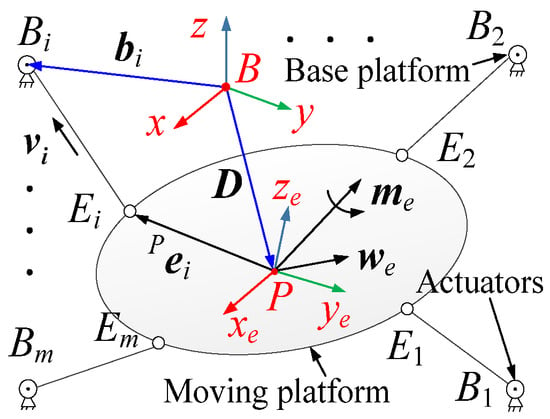
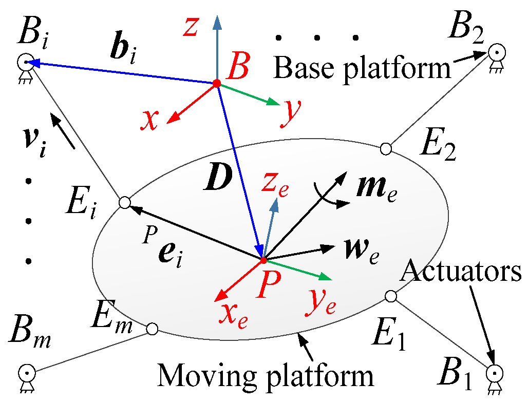
Figure 1 describes the schematic of the general CDPRs model, which can be controlled by using m-driven wires. The moving platform of robots is connected to the fixed actuators by using m-driven wires. The CDPRs’ moving and base coordinate frames are separately assigned by $P$ and $B$. Here, $E_i$ denotes the connection point between the moving platform and driven wires, and $B_i$ represents the fixed exit points of driven wires. By applying the above-mentioned two coordinate systems, the moving platforms’ posture and position can be expressed by using the angular displacement, $\mathsf{\Theta }={[\alpha ,\beta ,\gamma ]}^{\mathrm{T}}$ (in degree), of $P$ relative to $B$ and the position vector, and $\mathit{D}={[{\mathrm{x}}_{\mathrm{P}},{\mathrm{y}}_{\mathrm{P}},{\mathrm{z}}_{\mathrm{P}}]}^{\mathrm{T}}$ (in meters), of the origin of $P$ in $B$, respectively. Thus, $\mathit{x}={[D,\mathsf{\Theta }]}^{\mathrm{T}}$ is the moving platform’s pose in $B$. As the CDPRs’ dimension investigated in this work is small, the gravity of driven wires can usually be ignored, and the linear model of driven wires is used in the static balance. According to the cable catenary model [38], as the length and width of the robots in this paper are both less than 2 m, the deformation of the cable due to gravity can be ignored and a linear model is utilized instead of the cable catenary model.

Figure 1. The CDPRs’ general structural model.

By using the CDPRs’ static equilibrium condition, we can calculate the static equation as follows:

$${\displaystyle \sum _{i=1}^m{\mathsf{\tau }}_i}+{\mathit{w}}_e=0,{\displaystyle \sum _{i=1}^m{\mathbf{e}}_i\times {\mathsf{\tau }}_i}+{\mathit{m}}_e=0$$

(1)

where ${\mathsf{\tau }}_i$ denotes the tension of the ith driven wires, $\overrightarrow{{\mathit{E}}_{\mathit{i}}{\mathit{B}}_{\mathit{i}}}$ and ${\mathbf{e}}_i$ represent, separately, the direction of ${\mathsf{\tau }}_i$ and the vector $\overrightarrow{\mathit{P}{\mathit{E}}_{\mathit{i}}}$, and ${\mathit{m}}_e$ and ${\mathit{w}}_e$ are the resultant torque (N·m) and force (N) (containing the moving platform’s weight) of the load acting on the CDPRs, respectively. Let ${\mathsf{\tau }}_i$ be the magnitude of ${\mathsf{\tau }}_i$, and ${\mathit{v}}_i$ be the unit vector of the ith driven cables which has the same direction as ${\mathsf{\tau }}_i$. Moreover, ${\mathit{v}}_i$ can be calculated by $(\mathit{B}{\mathit{B}}_i-\mathit{B}\mathit{P}-\mathit{P}{\mathit{E}}_i)/(\mathit{B}{\mathit{B}}_i-\mathit{B}\mathit{P}-\mathit{P}{\mathit{E}}_i)=({\mathit{b}}_i-\mathit{D}-\Re \cdot {}^P\mathit{e}_i)/({\mathit{b}}_i-\mathit{D}-\Re \cdot {}^P\mathit{e}_i)$, where ${\mathit{b}}_i$ and ${}^P\mathit{e}_i$ are separately the position vector of $B_i$ in $B$ and $E_i$ in $P$, and $\Re$ is the rotation matrix of $P$ relative to $B$.

By using Equation (1), one can obtain

$${\displaystyle \mathbb{R}}·{\displaystyle \mathbb{C}}+\mathit{W}=0$$

(2)

where ${\displaystyle \mathbb{C}}={\left[{\tau }_1,{\tau }_2,\dots ,{\tau }_m\right]}^{\mathrm{T}}$ represents the cables tension vector, $\mathit{W}={\left[{\mathit{w}}_e,{\mathit{m}}_e\right]}^{\mathrm{T}}$, and ${\displaystyle \mathbb{R}}$ denotes the CDPRs’ structure matrix, where

$${\displaystyle \mathbb{R}}(\mathit{x})=\left[\begin{array}{l}\hspace{1em}\hspace{0.33em}\hspace{0.33em}\hspace{0.33em}\hspace{0.17em}{\mathit{v}}_1\hspace{1em}\hspace{1em}\hspace{0.33em}\hspace{0.33em}\hspace{0.33em}\dots \hspace{1em}\hspace{1em}\hspace{0.33em}\hspace{0.33em}\hspace{0.33em}\hspace{0.33em}{\mathit{v}}_m\\ (\Re \cdot {}^P\mathit{e}_1)\times {\mathit{v}}_1\hspace{1em}\dots \hspace{1em}(\Re \cdot {}^P\mathit{e}_m)\times {\mathit{v}}_m\end{array}\right].$$

2.2. Static Stiffness Model

This section first reviews the stiffness model previously studied in refs. [1,7]. When the external load acts on CDPRs, the robots’ anti-deformation ability is one of the indices that estimates the robots’ stiffness. The following mathematical expression of relationship between the small load, $\delta \mathit{W}$, applied to the CDPRs, and the small change, $\delta \mathit{x}$, of robots’ posture can be written:

$$\delta \mathit{W}=M\cdot \delta \mathit{x}$$

(3)

where $\mathit{M}$ represents the stiffness matrix.

By using Equations (2) and (3), we have

$$\mathit{M}=\partial \mathit{W}/\partial \mathit{x}=-((\partial {\displaystyle \mathbb{R}}/\partial \mathit{x}){\displaystyle \mathbb{C}}+{\displaystyle \mathbb{R}}(\partial {\displaystyle \mathbb{C}}/\partial \mathit{x}))={\mathit{M}}_1+{\mathit{M}}_2$$

(4)

As shown in Equation (4), the matrix $\mathit{M}$ contains two parts. ${\mathit{M}}_1$ is relevant to the driven wire tension and the robots’ structure matrix transformation, which can usually be controlled by using the driven wire tension and named as controllable stiffness. ${\mathit{M}}_2$ is relevant to the CDPRs’ structure and posture and named as inherent stiffness.

The basis of enabling robots to obtain the CSS is controllable stiffness. From (4), ${\mathit{M}}_1$ can be obtained:

$${\mathit{M}}_1=-\mathit{H}{\displaystyle \mathbb{C}}$$

(5)

where $\mathit{H}=[{\mathit{H}}^1,{\mathit{H}}^2,\dots ,{\mathit{H}}^n]\in {\mathrm{R}}^{n\times n\times m}$ is the Hessian matrix, and

$${\mathit{H}}^j={\displaystyle \frac{\partial {\displaystyle \mathbb{R}}}{\partial {\mathit{x}}_j}}=\left[\begin{array}{c}\partial {\mathit{v}}_1/\partial {\mathit{x}}_j\hspace{1em}\hspace{1em}\hspace{0.33em}\hspace{0.17em}\dots \hspace{0.33em}\hspace{1em}\hspace{1em}\hspace{0.33em}\partial {\mathit{v}}_m/\partial {\mathit{x}}_j\\ \partial [(\Re \cdot {}^P\mathit{e}_1)\times {\mathit{v}}_1]/\partial {\mathit{x}}_j\hspace{0.17em}\hspace{0.33em}\dots \hspace{0.17em}\hspace{0.33em}\partial [(\Re \cdot {}^P\mathit{e}_m)\times {\mathit{v}}_m]/\partial {\mathit{x}}_j\end{array}\right]$$

(6)

The inherent stiffness of robots cannot usually be controlled by using the driven wire tension, but it still shows a great influence on CDPRs’ stiffness. From Equation (4), ${\mathit{M}}_2$ can be obtained as follows:

$${\mathit{M}}_2=-{\displaystyle \mathbb{R}}{\displaystyle \frac{\partial {\displaystyle \mathbb{C}}}{\partial \mathit{l}}}{\displaystyle \frac{\partial \mathit{l}}{\partial \mathit{x}}}={\displaystyle \mathbb{R}}\cdot diag({\displaystyle \frac{{\mathrm{E}}_1\cdot {\mathrm{A}}_1}{l_{\mathrm{o}1}}},\dots ,{\displaystyle \frac{{\mathrm{E}}_m\cdot {\mathrm{A}}_m}{l_{\mathrm{o}\mathrm{m}}}})\cdot {{\displaystyle \mathbb{R}}}^T$$

(7)

where $l_{oi}$, $E_i$, and $A_i$ denote separately the static length, elastic modulus, and cross sectional area of the ith wire.

3. Constant Stiffness Space and Cable-Tension-Constrained Workspace

In this section, the concepts of the CSS and CTCW and their calculation methods are discussed. First, the CTFR of CDPRs is briefly reviewed [39].

3.1. Cable Tension Feasible Region

CDPRs’ performance is closely related to the tension of driven wires. Therefore, the CDPRs’ CTCW and CSS are investigated based on the CTFR in this paper. Next, when the robots’ load is constant, a 2 degree of redundancy CDPR is considered as a study case, and the CDPRs’ CTFR is explained as follows.

When the structure matrix is a full rank matrix, because this paper considers the CTFR for the 2 degree of redundancy CDPR, from Equation (2), the following expression is obtained:

$${\displaystyle \mathbb{C}}={{\displaystyle \mathbb{R}}}^{+}(-\mathit{W})+\mathit{U}\mathsf{\phi }= {\mathit{t}}_s+{\mathit{t}}_u$$

(8)

where ${{\displaystyle \mathbb{R}}}^{+}$ represents the Moore–Penrose pseudoinverse of ${\displaystyle \mathbb{R}}$, ${\mathit{U}}_{m\times 2}=\mathrm{null}({\displaystyle \mathbb{R}})$ represents a full rank matrix, $\mathsf{\phi }=[{\phi }_1 {\phi }_2{]}^{\mathrm{T}}$ denotes a 2D point, and ${\phi }_1\in \mathrm{R}$, ${\phi }_2\in \mathrm{R}$, and $\mathit{U}\mathsf{\phi }$ and ${{\displaystyle \mathbb{R}}}^{+}\left(-\mathit{W}\right)$ are the homogeneous general solution and the minimum-norm solution of Equation (2), respectively.

Let $\mathsf{\Pi }$ be the set of driven wire tension solutions, ${\displaystyle \mathbb{C}}$, of Equation (2) satisfying ${\tau }_{\min }\le {\displaystyle \mathbb{C}}\le {\tau }_{\max }$, which can usually be obtained by using the following 2 m inequalities:

$${\tau }_{\min }-{\mathit{t}}_s\le {\mathit{U}}_{m\times 2}\mathsf{\phi }\le {\tau }_{\max }-{\mathit{t}}_s$$

(9)

where ${\tau }_{\min }$ and ${\tau }_{\max }$ represent the lower and upper driven cables’ tension-limited value vectors of CDPRs, respectively. As $\mathsf{\phi }$ changes, each inequality can determine a half plane via utilizing a boundary line, when the critical values of driven wire tension are constant. The closed region obtained via the intersection of 2 m half planes, which can be determined through using Equation (9), is called the CTFR. In this work, robots are actuated through using m identical driven cables; therefore, the limiting values for each cable tension are the same.

3.2. Constant Stiffness Space

There are usually different demands for the CDPRs’ performance when they are used in different workplaces. For example, in simulation satellite Mars landing experiments, a workspace with a constant stiffness is usually required for the CDPRs [5]. The CDPRs’ CSS is usually a closed space with a constant system stiffness, which can be formed by robots’ posture set, whereas the driven cable tension of robots must be in the CTFR, and its mathematical expression can be obtained:

$$\begin{gathered} \mathrm{find}\hspace{1em}\hspace{1em}\hspace{0.33em}{\mathrm{S}}_c(x) \\ \mathrm{s}.\hspace{0.33em}\mathrm{t}.\hspace{0.33em}\hspace{1em}\mathrm{M}(x_i)={\mathrm{M}}_c \\ \hspace{0.17em}{\mathit{p}}_{\hspace{0.17em}x}\in \mathrm{CTFR}(x_i) \end{gathered}$$

(10)

where x represents the CDPRs’ set of postures, ${\mathrm{S}}_c(x)$ represents the CSS, $x_i$ denotes posture in the set x, $\mathrm{M}(x_i)$ denotes CDPRs’ system stiffness at the posture $x_i$, ${\mathrm{M}}_c$ denotes a stiffness matrix, ${\mathit{p}}_{\hspace{0.17em}x}$ denotes any point on the located plane of the $\mathrm{CTFR}(x_i)$, and $\mathrm{CTFR}(x_i)$ represents the CDPRs’ CTFR at the posture $x_i$.

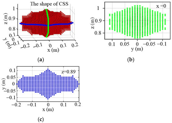
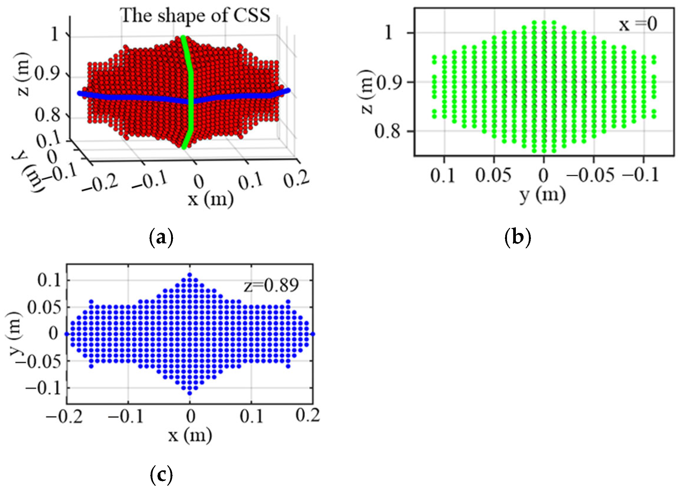
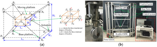
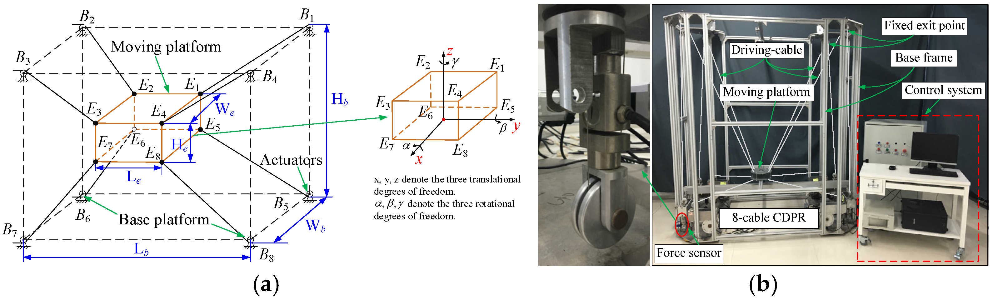
To effectively obtain the CDPRs’ CSS, its calculation method is introduced, as illustrated in Algorithm A1 in Appendix A. An example of the CSS is shown in Figure 2; the dimensions and configuration of CDPRs are depicted in Figure 3a and Table 1; and the performance parameters of driven cables are presented in Table 2; Figure 3b is the prototype system of CDPRs.

Figure 2. The example of the CSS. (a) The shape of the CSS. (b) The CSS’s cross section in the x direction. (c) The CSS’s cross section in the z direction.

Figure 3. The eight-cables-driven spatial 6-DOF CDPRs. (a) Framework diagram. (b) Prototype system.

Table 1. The dimensions of CDPRs.

Dimension	Value (Meters)	Dimension	Value (Meters)
${\mathrm{L}}_b$	$1.540$	${\mathrm{L}}_e$	$0.124\sqrt{2}$
${\mathrm{W}}_b$	$1.032$	${\mathrm{W}}_e$	$0.124\sqrt{2}$
${\mathrm{H}}_b$	$1.780$	${\mathrm{H}}_e$	$0.085$

Table 2. The performance parameter of driven cables.

Parameter	Description	Value
$E_s$	Yang’s Elastic Modulus of driven wires	12.4 GPa
$D$	Diameter of driven wires	0.47 mm
$t_{\max }$	Maximum cable tension	400 N
$t_{\min }$	Minimum cable tension	10 N

GPa = 10⁹ N/m²; mm = millimeter.

In this work, the step size $s_r=1$ mm, and the accuracy is $\epsilon =5\%$.

3.3. Cable-Tension-Constrained Workspace

The driven cable tension is closely related to the robots’ performance. Therefore, it is of great significance to study the robots’ CTCW. In practical applications, the cable materials of different CDPRs tend to have large differences, which results in a great difference in the limited values ${\tau }_{\min }$ and ${\tau }_{\max }$ of the driven cable tension (the material properties of the wires selected are shown in Table 2). The robot’s cable tension requirements for the driven cables often vary in different applications. Therefore, the driven cable tension of robots is required to be within a certain range. For this reason, the concept of CDPRs’ CTCW is proposed, and its calculation methods are presented in this work.

The CDPR is under the action of load while satisfying the system balance, and the closed area determined by the posture set of robots, whose driven cable tension is within the critical value range, and is called the cable-tension-constrained workspace (CTCW), which can be calculated as follows:

$$\begin{gathered} \mathrm{find}\hspace{1em}\hspace{1em}\hspace{1em}{\mathrm{S}}_t(x) \\ \mathrm{s}.\hspace{0.33em}\mathrm{t}.\hspace{0.33em}\hspace{1em}\hspace{0.33em}{\displaystyle \mathbb{R}}·{\displaystyle \mathbb{C}}+\mathit{W}=0 \\ \hspace{0.17em}{\displaystyle \mathbb{C}}\in [{\tau }_{\min },{\tau }_{\max }] \end{gathered}$$

(11)

where ${\mathrm{S}}_t(\mathrm{x})$ is the CTCW and x represents the CDPRs’ posture set.

At any posture, a redundant CDPR usually has numerous groups of driven cable tension vectors ${\displaystyle \mathbb{C}}$ satisfying ${\displaystyle \mathbb{R}}·{\displaystyle \mathbb{C}}+\mathit{W}=0$. Generally, these driven cable tension vectors of the CDPR can form an r-dimensional affine space. Therefore, it is difficult to acquire the optimal driven wire tension solutions satisfying ${\displaystyle \mathbb{R}}·{\displaystyle \mathbb{C}}+\mathit{W}=0$. However, as this paper applies the 2 degree of redundancy CDPRs, the CTFR is considered on a plane. By using Equation (11), the following expression can be obtained:

$$\begin{gathered} \mathrm{find}\hspace{1em}\hspace{1em}\hspace{1em}{\mathrm{S}}_t(x) \\ \mathrm{s}.\hspace{0.33em}\mathrm{t}.\hspace{0.33em}\hspace{1em}\mathrm{CTFR}(x_i)\notin \varnothing \end{gathered}$$

(12)

where $\mathrm{CTFR}({\mathrm{x}}_i)$ denotes the CDPRs’ CTFR at the posture ${\mathrm{x}}_i$.

Therefore, (12) can transform the iteration problem, which examines whether the CDPRs’ posture belongs to its CTCW, into the geometry problem, which examines whether the CDPRs’ CTFR exists. According to the above analysis, the computing method of the CDPRs’ CTCW is designed on the basis of the CTFR to effectively determine the CTCW. The detailed calculation process of the CTCW is illustrated in Algorithm A2 in Appendix A.

In this work, the step size $l_o=10\hspace{0.33em}\mathrm{mm}$. Different types of CTCWs of CDPRs can be obtained by modifying critical conditions of (11) based on the CTFR. The lowest power consumption CTCW, highest stiffness CTCW, and optimum safety CTCW can be acquired through constraining the driven wire tension.

4. Dimension and Shape Optimization

Generally, the CDPR can be rapidly reconstructed and quickly adjust its mechanical structure by using the modular design in order to fulfill various working demands. Therefore, it is significant to investigate the effects of the CDPR dimension and shape on its CSS and CTCW volume. In practical applications, since the CDPRs’ moving platform is usually non-point-mass, the driven cable tension generates extra torque on the robots. From (2), ${\mathit{W}}_c$ can be obtained:

$${\mathit{W}}_c={\displaystyle \mathbb{R}}·{\displaystyle \mathbb{C}}=\left[\begin{array}{l}\hspace{1em}\hspace{0.33em}\hspace{0.33em}\hspace{0.33em}{\mathit{v}}_1\hspace{1em}\hspace{1em}\hspace{0.33em}\hspace{0.17em}\dots \hspace{1em}\hspace{1em}\hspace{0.33em}\hspace{0.33em}\hspace{0.33em}\hspace{0.33em}{\mathit{v}}_m\\ e_1\cdot \sin {\theta }_1\cdot {\mathsf{\delta }}_1\hspace{0.33em}\dots \hspace{0.33em}{e}_m\cdot \sin {\theta }_m\cdot {\mathsf{\delta }}_m\end{array}\right]{\left[{\tau }_1,{\tau }_2,\dots ,{\tau }_m\right]}^{\mathrm{T}}$$

(13)

where ${\mathit{W}}_c={\left[{\mathit{w}}_c,{\mathit{m}}_c\right]}^{\mathrm{T}}$, and ${\mathit{m}}_c$ and ${\mathit{w}}_c$ denote the resultant torque (N·m) and force (N) acting on the CDPRs by using the driven wire tension of robots, respectively. ${\theta }_i$ represents the angle between ${\mathbf{e}}_i$ and ${\mathit{v}}_i$, and ${\mathsf{\delta }}_i$ represents the unit vector of $(\Re \cdot {}^P\mathit{e}_i)\times {\mathit{v}}_i$.

As shown in (13), it is clear that the torque of driven wire tension acting upon the robots is bound up with the posture (it can be determined according to different operation demands) and the shape of moving platform, and it is also bound up with the force arm $e_i$ of the driven cable tension. With an increase in the force arm $e_i$, the ${\mathsf{\tau }}_i\cdot e_i\cdot \sin {\theta }_i$ value also increases gradually. At a certain posture of CDPRs, the necessary and insufficient condition of this posture belongs to the CTCW or CSS is the driven cable tension satisfying ${\tau }_{\min }\le {\tau }_i\le {\tau }_{\max }$. Usually, the CDPRs cannot generate a small moment when $e_i$ is too large. Similarly, the CDPRs cannot generate large moment when $e_i$ is too small. Therefore, it is very important to investigate the dimension and configuration optimization of CDPRs’ basis platform and moving platform for improving the volume of the CTCW or CSS.

The spatial 6-DOF CDPR is usually driven by eight wires, and their configuration often adopts 4–4 configuration. As shown in Figure 3, the cable layout of these kinds of CDPRs is generally implemented in a symmetrical way, and their basis platform and moving platform are cubes. Due to a symmetrical mechanical structure, a large number of properties, such as working space, of this kind of CDPR are usually symmetrical. Moreover, many experts have also conducted numerous studies on such CDPRs, which are often employed for improving the performance of robots. Thus, this kind of CDPR is considered as a research object for studying the optimization problem of its shape and dimension in this work. The CDPRs’ dimension and shape are optimized by using the CSS and CTCW volume of robots as the optimization indicators in this work. Generally, the CDPRs’ dimension and shape display a significant impact on their CTCW and CSS volume, and there is also a definite proportion among the CDPRs’ dimensions. Any two structural dimensions of CDPR can form a ratio, which is referred to as the dimension coefficient (DC). Meanwhile, the effect of DCs on the CDPRs’ performance is mutually coupled. The global optimal result of the CDPRs’ dimension and shape is often difficult to obtain by the superposition of the single optimal variables, which can be determined by using the control variable optimization method. Therefore, the CDPRs’ dimension and shape are optimized through comprehensively considering the coupling effect of all DCs on the volume of robots’ CSS and CTCW.

4.1. Optimization Model of the CSS

Assume that $V_c$ denotes the volume of CDPRs’ CSS, which can be expressed as follows:

$$V_c=f({\epsilon }_1,{\epsilon }_2,{\epsilon }_3,{\epsilon }_4,{\epsilon }_5)$$

(14)

where ${\epsilon }_1={\mathrm{L}}_b/{\mathrm{L}}_e,{\epsilon }_2={\mathrm{W}}_b/{\mathrm{W}}_e,{\epsilon }_3={\mathrm{H}}_b/{\mathrm{H}}_e,{\epsilon }_4={\mathrm{L}}_b/{\mathrm{W}}_b,{\epsilon }_5={\mathrm{L}}_b/{\mathrm{H}}_b$, where ${\epsilon }_i(i=1,2,\dots ,5)$ is the DC; ${\mathrm{L}}_e({\mathrm{E}}_1{\mathrm{E}}_2)$, ${\mathrm{W}}_e({\mathrm{E}}_2{\mathrm{E}}_3)$, and ${\mathrm{H}}_e({\mathrm{E}}_2{\mathrm{E}}_6)$ are separately the length, width, and height of the cuboid enveloped via the junction point between driven cables and the moving platform; and ${\mathrm{L}}_b({\mathrm{B}}_1{\mathrm{B}}_2)$, ${\mathrm{W}}_b({\mathrm{B}}_2{\mathrm{B}}_3)$, and ${\mathrm{H}}_b({\mathrm{B}}_2{\mathrm{B}}_6)$ denote the length, width, and height of the cuboid enveloped through the fixed exit point of the driven wires, respectively. In addition, for an already designed CDPR, in order to obtain its optimum dimension and shape, we can optionally modify the junction points between the driven cables and moving platform, or the position of the fixed exit point of driven wires on the basis platform. Therefore, optimizing a mature CDPR product does not require modifying the dimension and shape of the basis platform. Generally, the CDPRs’ dimension and shape can be obtained through determining a structural dimension once the CDPRs’ DCs are determined.

In this work, the CDPRs’ limited size, ${\mathrm{H}}_b$(${\mathrm{H}}_b=1.78\hspace{0.17em}\mathrm{m}$), is considered. The CDPRs’ dimension and shape are optimized by using the DCs, considering the maximum CSS volume as performance indices. Therefore, in order to describe the CDPRs’ optimization problem, we have

$$\begin{gathered} \max \hspace{1em}\hspace{1em}\hspace{1em}\hspace{1em}\hspace{1em}{V}_c(\epsilon ) \\ \mathrm{s}.\hspace{0.33em}\mathrm{t}.\hspace{0.33em}\hspace{0.33em}\hspace{0.33em}\hspace{0.33em}\hspace{1em}\hspace{1em}\hspace{1em}\hspace{0.17em}{\varphi }_i\le {\epsilon }_i\le {\vartheta }_i \end{gathered}$$

(15)

where $V_c(\epsilon )$ represents the CSS volume, and ${\vartheta }_i$ and ${\varphi }_i$ are separately the DCs’ maximum and minimum limited values.

The CDPRs’ dimension and shape are optimized by using the response surface optimization model, which is established through comprehensively considering the coupling effect of each DC on the robots’ CSS volume. At the same time, the quadratic polynomial is used as the response surface optimization model in this work so that it can reflect the actual values of the CSS volume without too much complexity; thus, one can obtain

$$V_{cp}(\epsilon )={\displaystyle \sum _{i=1}^n{\delta }_i\cdot {\epsilon }_i}+{\displaystyle \sum _{k=1}^n{\displaystyle \sum _{i=k}^n{\delta }_{ki}\cdot {\epsilon }_k\cdot {\epsilon }_i}}+{\delta }_0$$

(16)

where $V_{cp}(\epsilon )$ is the predicted values of the CDPRs’ CSS volume, ${\epsilon }_i$ denotes the ith DC, and ${\delta }_i$, ${\delta }_{ki}$, and ${\delta }_0$ represent the response surface optimization model’s coefficients, which can be obtained through utilizing the least-squares method.

4.2. Optimization Model of the CTCW

In this work, assume that $V_t$ represents the CTCW volume of CDPRs, which can be expressed as follows:

$$V_t=g({\epsilon }_1,{\epsilon }_2,{\epsilon }_3,{\epsilon }_4,{\epsilon }_5)$$

(17)

Similarly to the CSS, optimizing already designed CDPRs does not require modifying the dimension and shape of the basis platform. The optimization problem of CDPRs considering the CTCW volume as the performance index is expressed as follows:

$$\begin{gathered} \max \hspace{1em}\hspace{1em}\hspace{1em}\hspace{1em}\hspace{1em}{V}_t(\epsilon ) \\ \mathrm{s}.\hspace{0.33em}\mathrm{t}.\hspace{0.33em}\hspace{0.33em}\hspace{0.33em}\hspace{1em}\hspace{1em}\hspace{1em}\hspace{0.33em}\hspace{0.17em}{\varphi }_i\le {\epsilon }_i\le {\vartheta }_i \end{gathered}$$

(18)

where $V_t(\epsilon )$ denotes the CTCW’s volume.

Similarly, the CDPRs’ dimension and shape are optimized by using the response surface optimization model, which is established through comprehensively considering the coupling effect of DCs on the CDPRs’ CTCW volume. Similarly to the CSS, the quadratic polynomial is used as the response surface optimization model so that it can effectively reflect the actual values of the CTCW volume; we have

$$V_{tp}(\epsilon )={\displaystyle \sum _{i=1}^n{\kappa }_i\cdot {\epsilon }_i}+{\displaystyle \sum _{k=1}^n{\displaystyle \sum _{i=k}^n{\kappa }_{ki}\cdot {\epsilon }_k\cdot {\epsilon }_i}}+{\kappa }_0$$

(19)

where $V_{tp}(\epsilon )$ is the predicted volume of the CDPRs’ CTCW, ${\epsilon }_i$ denotes the ith DC, and ${\kappa }_i$, ${\kappa }_{ki}$, and ${\kappa }_0$ represent the response surface optimization model’s coefficients, which can be obtained through utilizing the least-squares method.

5. Experimental Analysis and Optimization

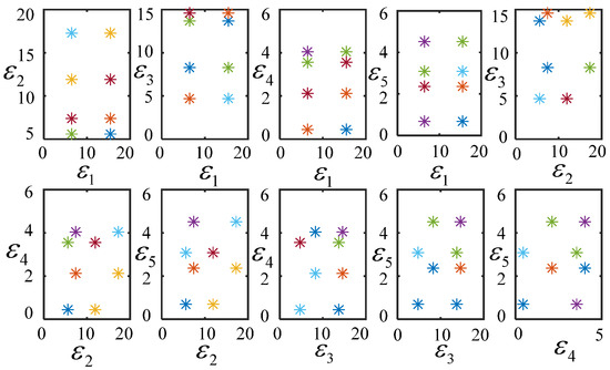
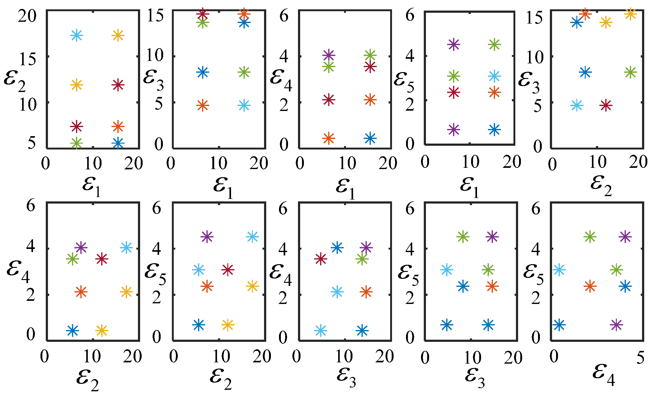
In this work, for optimizing the CDPRs’ dimension and shape by using the ideal response surface optimization model, the coefficients in (16) and (19) are determined by using the design of experiment (DOE) method. Generally, the approximation accuracy of the response surface optimization model is found relevant for the selected sample points. Meanwhile, the CDPRs have multiple variables that are required to be optimized and analyzed, their form of optimization targets (the shape of the CSS and CTCW) is usually irregular, and it is also difficult to gain the ideal result by using some experimental points, which are selected by simply using central composite design method or Box–Benhnken. Fortunately, the users can artificially set the number of sample points by using the Latin hypercube design method. The higher precision response surface optimization model can be obtained by using very few sample points because they apply the equal probability orthogonal distribution principle. Therefore, the positions of the sample points can be determined via utilizing the Latin hypercube design method in this paper. According to the empirical knowledge and practical engineering requirements, the DCs’ limited values (unit is 1) presented in Table 3 are used to investigate the optimization problem of the robots’ dimension and shape. When the CDPRs’ pose is $x={[0.0,0.0,{\mathrm{H}}_b(1-1/20),0.0,0.0,0.0]}^{\mathrm{T}}$, and the load of the moving platform is 0.0, the stiffness matrix of CDPRs, which is driven through using the tension of driven cables at the centroid of CTFR, is used as the stiffness matrix of CSS. According to the equal probability principle, this work divides the defined domain of DCs into two non-overlapping intervals, randomly selects the numbers in each interval, and randomly combines these numbers into a sample. Then, another sample can be obtained from the above intervals in the same way. As plotted in Figure 4, the singular points in both samples are removed, and the rest of the sample points are mixed together as an experimental sample.

Table 3. The limited values of the DCs.

Limited Values	${\mathit{\epsilon }}_1$	${\mathit{\epsilon }}_2$	${\mathit{\epsilon }}_3$	${\mathit{\epsilon }}_4$	${\mathit{\epsilon }}_5$
$\varphi$	2	2	2	0.2	0.2
$\vartheta$	20	20	20	5	5

Figure 4. Sample points selected by using the Latin hypercube design method.

Combining the sample points illustrated in Figure 4, the least-squares method is used to fit and solve (16), and thus the second-order polynomial response surface optimization model can be expressed as follows:

$$\begin{array}{l}{V}_{cp}(\epsilon )=84.4+38.4{\epsilon }_1-22.1{\epsilon }_2-20.7{\epsilon }_3-133.8{\epsilon }_4+95.9{\epsilon }_5-21.3{\epsilon }_1{\epsilon }_2+4.9{\epsilon }_1{\epsilon }_3-9.4{\epsilon }_1{\epsilon }_4+35.6{\epsilon }_1{\epsilon }_5-\\ 42.0{\epsilon }_2{\epsilon }_3-22.6{\epsilon }_2{\epsilon }_4-21.0{\epsilon }_2{\epsilon }_5+9.8{\epsilon }_3{\epsilon }_4-52.6{\epsilon }_3{\epsilon }_5-142.7{\epsilon }_4{\epsilon }_5-42.9{\epsilon }_2^2+33.7{\epsilon }_3^2+20.9{\epsilon }_4^2+106.1{\epsilon }_5^2\end{array}$$

(20)

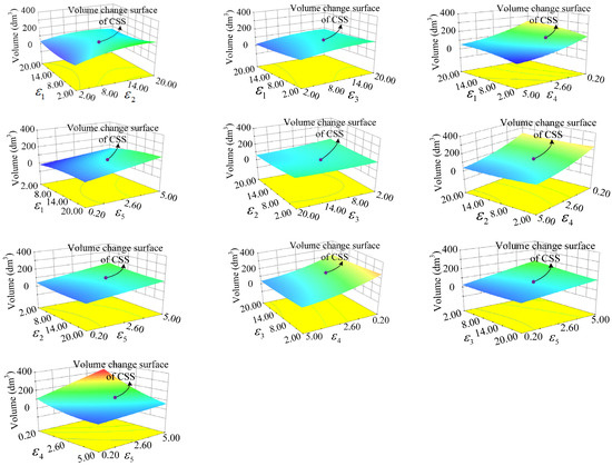
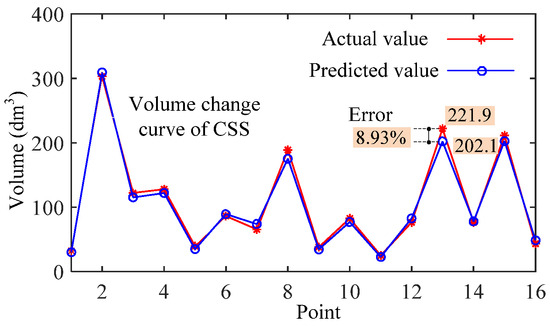
Then, the response surface gained by using the above model is described in Figure 5, and some typical points are selected for comparing the predicted value with the actual value, as shown in Figure 6 and Table 4.

Figure 5. Response surface model of the CSS.

Figure 6. The contrast curve of the predicted volume and actual volume of the CSS.

Table 4. Comparison of the predicted volume and actual volume of the CSS.

CSS Volume		Relative Errors	CSS Volume		Relative Errors
Actual Values	Predicted Values		Actual Values	Predicted Values
32.272	30.344	5.97%	37.992	34.636	8.83%
302.8	309.163	2.10%	82.6	77.155	6.59%
122.304	115.252	5.77%	25.216	22.855	9.36%
127.976	121.989	4.68%	76.488	82.821	8.28%
39.464	34.987	11.34%	221.92	202.092	8.93%
86.344	89.243	3.36%	76.688	77.973	1.68%
65.632	73.669	12.25%	211.728	202.860	4.19%
189.176	175.475	7.24%	37.992	34.636	13.12%

In this paper, dm denotes decimeter.

The results from Figure 5 are that the variation of ${\epsilon }_1$, ${\epsilon }_2$, and ${\epsilon }_3$ shows small effect on the robots’ CSS volume with the height ${\mathrm{H}}_b=1.78\hspace{0.17em}\mathrm{m}$ of the basis platform. However, the variation of ${\epsilon }_4$ and ${\epsilon }_5$ shows a significant impact on the CDPR’s CSS volume. The CSS’s volume gradually increases with a decrease in ${\epsilon }_4$ and an increase in ${\epsilon }_5$. The values of Adj R-squared $R_{adj}^2(0.8011>0.8)$ and R-squared $R^2(0.8674>0.8)$ of the above-mentioned model are very close, and they are also very close to 1, which indicate that the designed model can predict the CSS’s volume well. The results shown in Table 4 indicate that the maximum relative error between the actual volume and predicted volume of the CDPRs’ CSS is 13.12%, and the average relative error is 7.11%, which fulfills the design requirement with the average relative prediction error of less than 10%. As illustrated in Figure 6, the actual values of CDPRs’ CSS volume show good coherence with the predicted values of the model, which further verifies the validity of the response surface model constructed in this work. The optimal DCs can be obtained by using the response surface analysis and experimentally and comprehensively considering the DCs’ coupling influence on the robots’ CSS volume, and the optimization results are presented in Table 5.

Table 5. The optimization results considering the CSS’s volume as the performance indicator.

${\mathit{\epsilon }}_1$	${\mathit{\epsilon }}_2$	${\mathit{\epsilon }}_3$	${\mathit{\epsilon }}_4$	${\mathit{\epsilon }}_5$	V (dm3)
19.47	14.38	2.11	0.64	3.89	480.32

Similarly, combining the sample points illustrated in Figure 4, the least-squares method is used to fit and solve (19), and the second-order polynomial response surface optimization model is expressed as follows:

$$\begin{array}{l}{V}_{tp}(\epsilon )=3647.9-569.5{\epsilon }_1+53.4{\epsilon }_2+454.3{\epsilon }_3-5823.6{\epsilon }_4+5426.5{\epsilon }_5+130.9{\epsilon }_1{\epsilon }_2-664.3{\epsilon }_1{\epsilon }_3\\ +697.0{\epsilon }_1{\epsilon }_4-740.2{\epsilon }_1{\epsilon }_5-1303.4{\epsilon }_2{\epsilon }_3-23.6{\epsilon }_2{\epsilon }_4+75.2{\epsilon }_2{\epsilon }_5-698.3{\epsilon }_3{\epsilon }_4+1318.8{\epsilon }_3{\epsilon }_5\\ -10612.9{\epsilon }_4{\epsilon }_5-374.9{\epsilon }_2^2-505.2{\epsilon }_3^2-2223.6{\epsilon }_4^2+7373.5{\epsilon }_5^2\end{array}$$

(21)

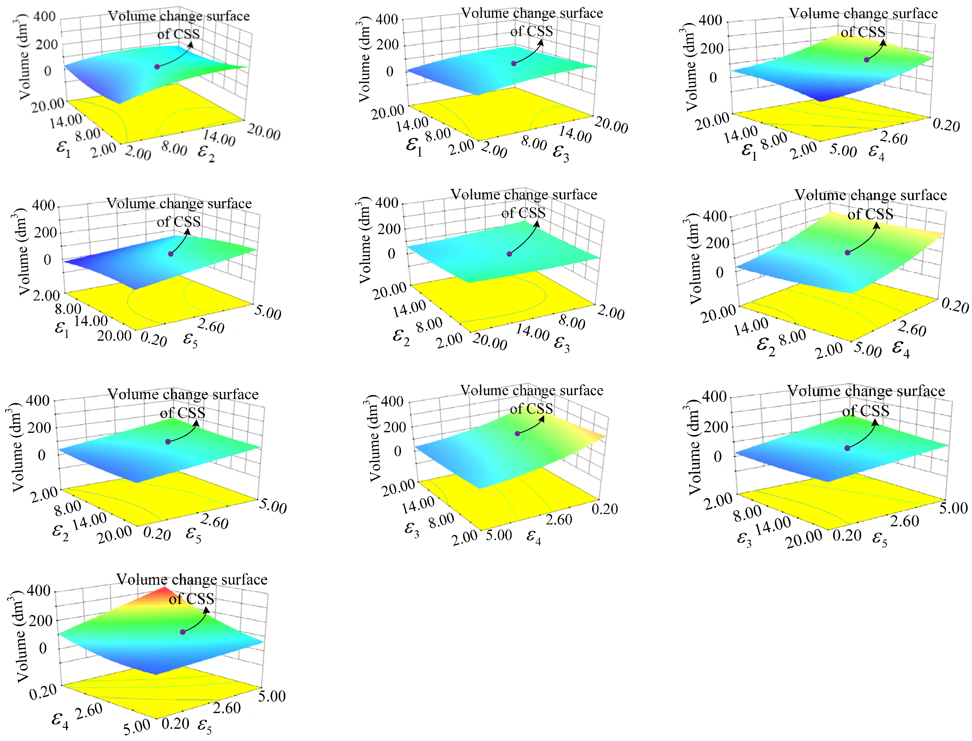
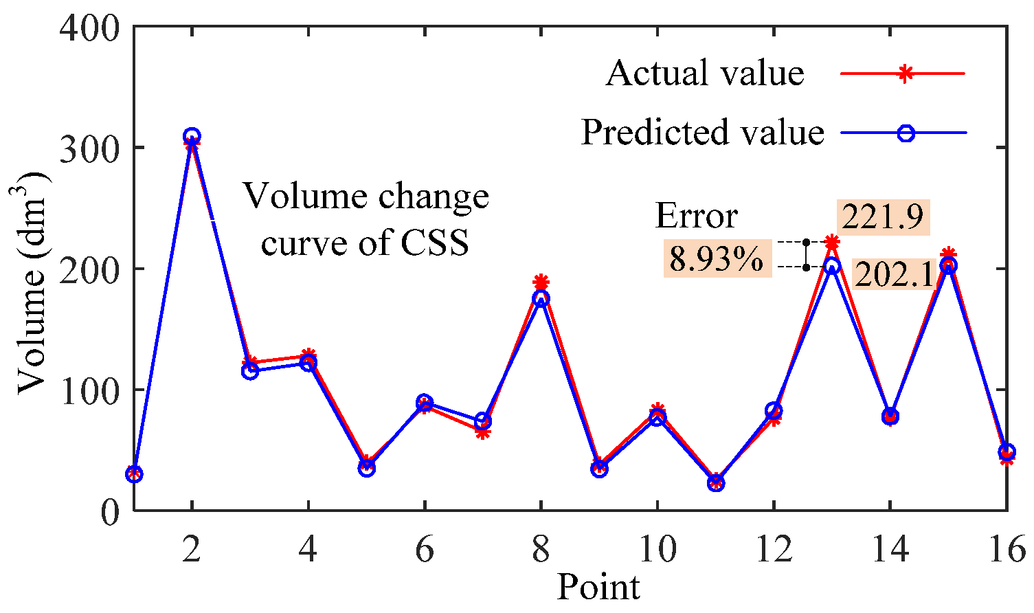
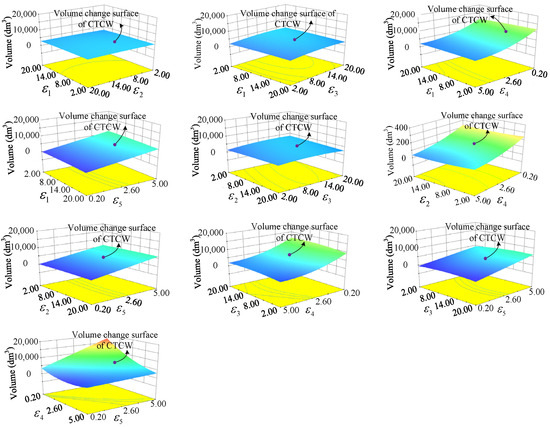
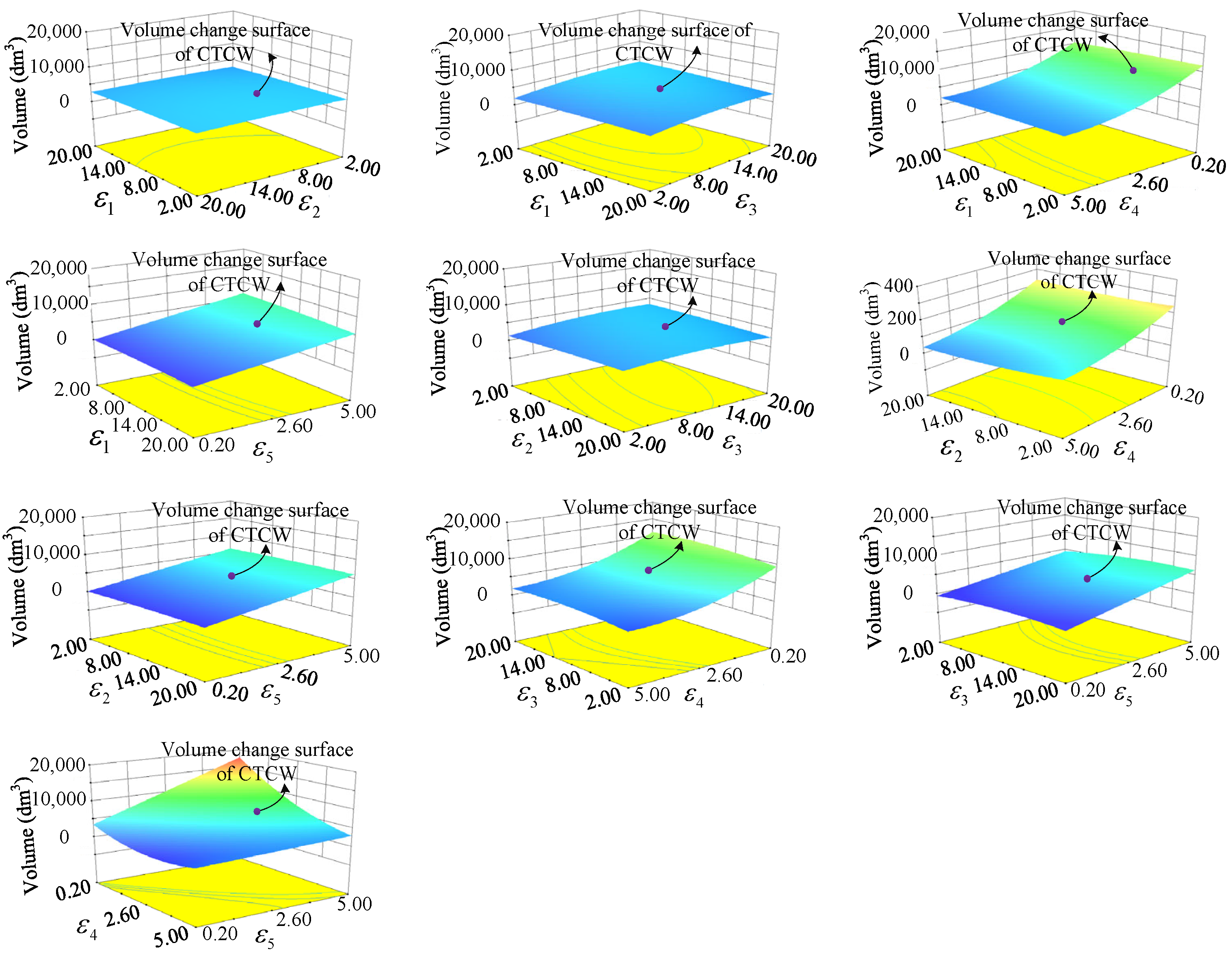
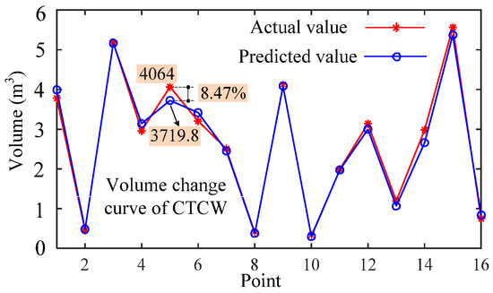
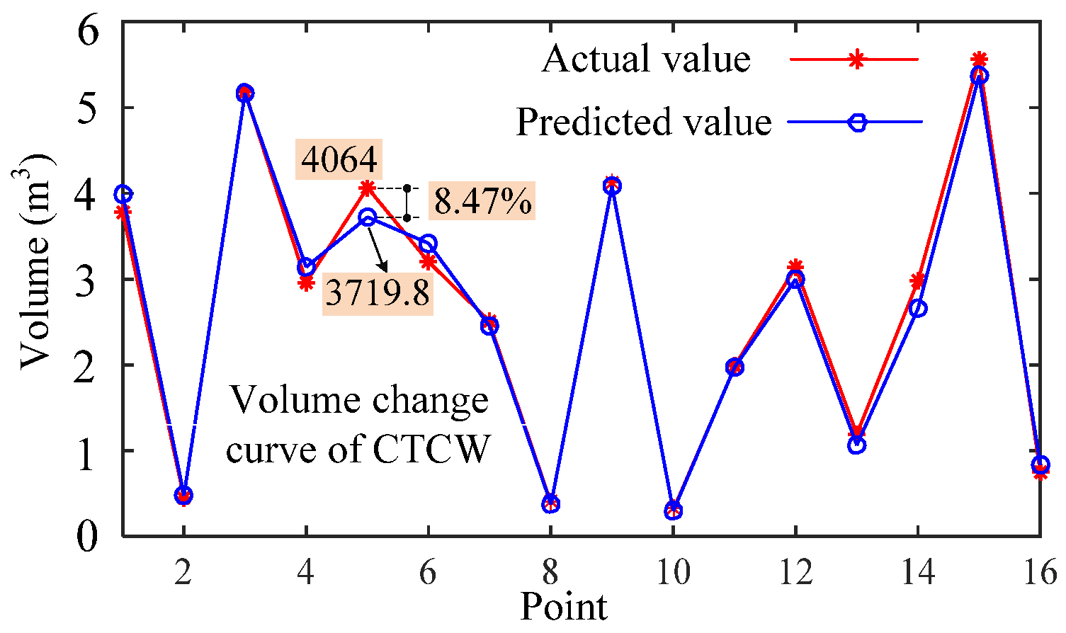
Then, the response surface can be obtained by using the above model, as shown in Figure 7, and some typical points are selected for comparing the predicted value with the actual value, as shown in Figure 8 and Table 6.

Figure 7. Response surface model of the CTCW.

Figure 8. The contrast curve of the predicted volume and actual volume of the CTCW.

Table 6. Comparison of the predicted volume and actual volume of the CTCW.

CTCW Volume		Relative Errors	CTCW Volume		Relative Errors
Actual Values	Predicted Values		Actual Values	Predicted Values
3776	3987.222	5.59%	4128	4082.515	1.10%
448	476.984	6.47%	328	293.929	10.39%
5184	5164.817	0.37%	1984	1970.871	0.66%
2960	3138.541	6.03%	3136	2994.574	4.51%
4064	3719.803	8.47%	1192	1062.488	10.86%
3200	3415.268	6.73%	2984	2656.680	10.97%
2504	2447.499	2.26%	5560	5369.606	3.42%
408	371.765	8.88%	744	830.481	11.62%

Similarly, the results shown from Figure 7 are that the variation of ${\epsilon }_1$, ${\epsilon }_2$, and ${\epsilon }_3$ shows small impact on the CDPRs’ CTCW volume with the height ${\mathrm{H}}_b=1.78\hspace{0.17em}\mathrm{m}$ of the basis platform. The variation of ${\epsilon }_4$ and ${\epsilon }_5$ shows a significant effect on the CDPRs’ CTCW volume. The CDPRs’ CTCW volume gradually increases with a decrease in ${\epsilon }_4$ and an increase in ${\epsilon }_5$. The values of Adj R-squared $R_{adj}^2(0.9612>0.8)$ and R-squared $R^2(0.9741>0.8)$ of the above-mentioned model are very close, and they are also very close to 1, which indicate that the designed model can predict the CTCW’s volume well. The results shown from Table 6 indicate that the maximum relative error between the predicted volume and actual volume of CDPRs’ CTCW is 11.62%, and the average relative error is 6.14%, which fulfills the design requirement with the average relative prediction error of less than 10%. As can be seen from Figure 8, the actual values of CDPRs’ CTCW volume show good coherence with the predicted values of the model, which further verifies the validity of the response surface model established in this paper. The optimal DCs can be obtained by using the response surface analysis and experimentally and comprehensively considering the DCs’ coupling impact on the CTCW volume of CDPRs, and the optimization results are presented in Table 7.

Table 7. The optimization results considering the CTCW volume as the performance index.

${\mathit{\xi }}_1$	${\mathit{\xi }}_2$	${\mathit{\xi }}_3$	${\mathit{\xi }}_4$	${\mathit{\xi }}_5$	V (dm3)
5.72	2.58	17.92	0.46	4.72	29,988.9

6. Conclusions

In this work, the eight-cables-driven spatial 6-DOF parallel robots are considered as a research object. First, the CDPRs’ static model is developed by using the static analysis, and the previously researched CDPRs’ CTFR and stiffness models are reviewed. Next, the concepts of the CSS and CTCW and their calculation methods are introduced, and the CSS and CTCW volume are considered as the optimization performance indices of CDPRs. The response surface optimization model between multi-objective optimization variables and CDPRs’ workspace volume is established by comprehensively considering the intercoupling relationship of optimization variables and their effect on CDPRs’ workspace volume, and combined with the selected sample points; it is solved by using the Latin hypercube design method. Then, by comprehensively considering the intercoupling impact of DCs on the robots’ CSS and CTCW volume, the CDPRs’ dimension and shape are optimized by using the constructed response surface model, and some typical points are selected and their actual and predicted values are compared and analyzed. It can be found that the average relative error between the actual volume and predicted volume of the CSS is 7.11%, the average relative error between the actual volume and predicted volume of the CTCW is 6.14%, and they fulfill the design requirements with the average relative error of less than 10%. The CDPRs’ optimal dimension and shape are obtained with the maximum CSS and CTCW volume, respectively, as the performance indicators are given.

This work is described by considering the dimension and shape optimization of the eight-cables-driven spatial 6-DOF parallel mechanisms as the study object. Such CDPRs are widely used and highly favored in the academic or industrial fields, but they still do not contain all possible robot designs. However, our findings in this paper can also be applied or served as a reference for the optimization of other robots. In addition, the proposed multi-objective optimization model achieves the optimization of multiple parameters while ensuring parameter continuity. However, it still fails to include all other parameters that may affect robot performance, such as the dexterity and uniformity of the robot’s movement. Therefore, to better optimize the robot’s structural parameters and maintain better performance, in the future, we will take into account more factors affecting robot performance and conduct optimization analysis of the robot’s structural parameters.

References

- Cui, Z.; Tang, X.; Hou, S.; Sun, H. Research on controllable stiffness of redundant cable-driven parallel robots. IEEE/ASME Trans. Mechatron. 2018, 23, 2390–2401. [Google Scholar] [CrossRef] [Scilit]
- An, H.; Yuan, H.; Tang, K.; Xu, W.; Wang, X. A Novel Cable-Driven Parallel Robot with Movable Anchor Points Capable for Obstacle Environments. IEEE/ASME Trans. Mechatron. 2022, 27, 5472–5483. [Google Scholar] [CrossRef] [Scilit]
- Lu, Y.; Chang, Z.; Lu, Y.; Wang, Y. Development and kinematics/statics analysis of rigid-flexible-soft hybrid finger mechanism with standard force sensor. Robot. Comput.-Integr. Manuf. 2021, 67, 101978. [Google Scholar] [CrossRef] [Scilit]
- Fabritius, M.; Miermeister, P.; Kraus, W.; Pott, A. A framework for analyzing the accuracy, complexity, and long-term performance of cable-driven parallel robot models. Mech. Mach. Theory 2023, 185, 105331. [Google Scholar] [CrossRef] [Scilit]
- Merlet, J.P. Simulation of discrete-time controlled cable-driven parallel robots on a trajectory. IEEE Trans. Robot. 2017, 33, 675–688. [Google Scholar] [CrossRef] [Scilit]
- Shi, D.; Wang, L.; Zhang, Y.; Zhang, W.; Xiao, H.; Ding, X. Review of human—Robot coordination control for rehabilitation based on motor function evaluation. Front. Mech. Eng. 2022, 17, 28. [Google Scholar] [CrossRef] [Scilit]
- Cui, Z.; Tang, X.; Hou, S.; Sun, H. Calculation and analysis of constant stiffness space for redundant cable-driven parallel robots. IEEE Access 2019, 7, 75407–75419. [Google Scholar] [CrossRef] [Scilit]
- Zhang, Z.; Shao, Z.; You, Z.; Tang, X.; Zi, B.; Yang, G.; Gosselin, C.; Caro, S. State-of-the-art on theories and applications of cable-driven parallel robots. Front. Mech. Eng. 2022, 17, 37. [Google Scholar] [CrossRef] [Scilit]
- Wang, R.; Li, S.; Li, Y. A Suspended Cable-Driven Parallel Robot with Articulated Reconfigurable Moving Platform for Schönflies Motions. IEEE/ASME Trans. Mechatron. 2022, 27, 5173–5184. [Google Scholar] [CrossRef] [Scilit]
- Cheng, H.H.; Lau, D. Cable Attachment Optimization for Reconfigurable Cable-Driven Parallel Robots Based on Various Workspace Conditions. IEEE Trans. Robot. 2023, 39, 3759–3775. [Google Scholar] [CrossRef] [Scilit]
- Qian, W.; Liao, J.; Lu, L.; Ai, L.; Li, M.; Xiao, X.; Guo, Z. CURER: A Lightweight Cable-Driven Compliant Upper Limb Rehabilitation Exoskeleton Robot. IEEE/ASME Trans. Mechatron. 2023, 28, 1730–1741. [Google Scholar] [CrossRef] [Scilit]
- Zhong, B.; Shen, M.; Liu, H.; Zhao, Y.; Qian, Q.; Wang, W.; Yu, H.; Zhang, M. A Cable-Driven Exoskeleton with Personalized Assistance Improves the Gait Metrics of People in Subacute Stroke. IEEE Trans. Neural Syst. Rehabil. Eng. 2023, 31, 2560–2569. [Google Scholar] [CrossRef] [Scilit]
- Li, X.; Yang, Q.; Song, R. Performance-Based Hybrid Control of a Cable-Driven Upper-Limb Rehabilitation Robot. IEEE Trans. Biomed. Eng. 2021, 68, 1351–1359. [Google Scholar] [CrossRef] [Scilit]
- Hamida, I.B.; Laribi, M.A.; Mlika, A.; Romdhane, L.; Zeghloul, S.; Carbone, G. Multi-Objective optimal design of a cable driven parallel robot for rehabilitation tasks. Mech. Mach. Theory 2021, 156, 104141. [Google Scholar] [CrossRef] [Scilit]
- Cui, Z.; Li, W.; Zhang, X.; Chiu, P.W.Y.; Li, Z. Accelerated Dual Neural Network Controller for Visual Servoing of Flexible Endoscopic Robot with Tracking Error, Joint Motion, and RCM Constraints. IEEE Trans. Ind. Electron. 2022, 69, 9246–9257. [Google Scholar] [CrossRef] [Scilit]
- Hao, J.; Zhang, K.; Zhang, Z.; Wang, S.; Shi, C. An Online Model-Free Adaptive Tracking Controller for Cable-Driven Medical Continuum Manipulators. IEEE Trans. Med. Robot. Bionics 2023, 5, 623–635. [Google Scholar] [CrossRef] [Scilit]
- Li, Z.; Wu, L.; Ren, H.; Yu, H. Kinematic comparison of surgical tendon-driven manipulators and concentric tube manipulators. Mech. Mach. Theory 2017, 107, 148–165. [Google Scholar] [CrossRef] [Scilit]
- Nägele, F.; Halt, L.; Tenbrock, P.; Pott, A. A Prototype-Based Skill Model for Specifying Robotic Assembly Tasks. In Proceedings of the 2018 IEEE International Conference on Robotics and Automation (ICRA), Brisbane, Australia, 21–25 May 2018; pp. 558–565. [Google Scholar]
- Schmidt, A.; Martin, C.; Dietz, T.; Pott, A. A generic data structure for the specific domain of robotic arc welding. Procedia CIRP 2018, 72, 322–327. [Google Scholar] [CrossRef] [Scilit]
- Duan, J.; Liu, H.; Zhang, Z.; Shao, Z.; Meng, X.; Lv, J.; Huang, M. Reconfiguration and Performance Evaluation of TBot Cable-Driven Parallel Robot. J. Mech. Robot. 2025, 17, 010909. [Google Scholar] [CrossRef] [Scilit]
- Lin, J.; Chiang, C.K. Motion control of a cable-suspended robot using image recognition with coordinate transformation. Proc. Inst. Mech. Eng. Part I J. Syst. Control Eng. 2021, 235, 52–67. [Google Scholar] [CrossRef] [Scilit]
- Tadokoro, S.; Murao, Y.; Hiller, M.; Murata, R.; Kohkawa, H. A motion base with 6-DOF by parallel cable drive architecture. IEEE/ASME Trans. Mechatron. 2002, 7, 115–123. [Google Scholar]
- Nasr, A.; Moosavian, S.A.A. Multi-criteria design of 6-dof fully-constrained cable driven redundant parallel manipulator. In Proceedings of the IEEE 2015 3rd RSI International Conference on Robotics and Mechatronics (ICROM), Tehran, Iran, 7–9 October 2015; pp. 001–006. [Google Scholar]
- Seon, J.A.; Park, S.; Ko, S.Y.; Park, J.O. Cable configuration analysis to increase the rotational range of suspended 6-DOF cable driven parallel robots. In Proceedings of the IEEE 16th International Conference on Control, Automation and Systems (ICCAS), Gyeongju, Republic of Korea, 16–19 October 2016; pp. 1047–1052. [Google Scholar]
- Chellal, R.; Laroche, E.; Cuvillon, L. An H∞ methodology for position control of 6-DoF cable-driven parallel robots. In Proceedings of the IEEE European Control Conference (ECC), Strasbourg, France, 24–27 June 2014; pp. 358–363. [Google Scholar]
- Lau, D.; Oetomo, D.; Halgamuge, S.K. Wrench-closure workspace generation for cable driven parallel manipulators using a hybrid analytical-numerical approach. J. Mech. Des. 2011, 133, 071004. [Google Scholar]
- Azizian, K.; Cardou, P.; Moore, B. Classifying the boundaries of the wrench-closure workspace of planar parallel cable-driven mechanisms by visual inspection. J. Mech. Robot. 2012, 4, 024503. [Google Scholar] [CrossRef] [Scilit]
- Pham, C.B.; Yeo, S.H.; Yang, G.; Kurbanhusen, M.S.; Chen, I.M. Force-closure workspace analysis of cable-driven parallel mechanisms. Mech. Mach. Theory 2006, 41, 53–69. [Google Scholar]
- Barrette, G.; Gosselin, C. Determination of the dynamic workspace of cable-driven planar parallel mechanisms. J. Mech. Des. 2005, 127, 242–248. [Google Scholar] [CrossRef] [Scilit]
- Lamine, H.; Bennour, S.; Romdhane, L. Design of cable-driven parallel manipulators for a specific workspace using interval analysis. Adv. Robot. 2016, 30, 585–594. [Google Scholar] [CrossRef] [Scilit]
- Jamshidifar, H.; Khajepour, A. Static Workspace Optimization of Aerial Cable Towed Robots with Land-Fixed Winches. IEEE Trans. Robot. 2020, 36, 1603–1610. [Google Scholar] [CrossRef] [Scilit]
- Zhang, Z.; Shao, Z.; Wang, L. Optimization and implementation of a high-speed 3-DOFs translational cable-driven parallel robot. Mech. Mach. Theory 2020, 145, 103693. [Google Scholar] [CrossRef] [Scilit]
- Bolboli, J.; Khosravi, M.A.; Abdollahi, F. Stiffness feasible workspace of cable-driven parallel robots with application to optimal design of a planar cable robot. Robot. Auton. Syst. 2019, 114, 19–28. [Google Scholar] [CrossRef] [Scilit]
- Hay, A.M.; Snyman, J.A. Optimization of a planar tendon-driven parallel manipulator for a maximal dextrous workspace. Eng. Optim. 2005, 37, 217–236. [Google Scholar] [CrossRef] [Scilit]
- Jiang, X.; Huang, Y.; Zheng, Y. Dimension optimization design of an under-restrained 6-DOF four-cable-driven parallel manipulator based on least square-support vector regression. In Proceedings of the IEEE International Conference on Mechatronics and Automation, Beijing, China, 7–10 August 2011; pp. 458–463. [Google Scholar]
- Zhang, D.; Gao, Z. Forward kinematics, performance analysis, and multi-objective optimization of a bio-inspired parallel manipulator. Robot. Comput.-Integr. Manuf. 2012, 28, 484–492. [Google Scholar] [CrossRef] [Scilit]
- Cui, Z.; Tang, X.; Hou, S.; Sun, H. Optimization Design of Redundant Cable Driven Parallel Robots Based on Constant Stiffness Space. In Proceedings of the IEEE International Conference on Robotics and Biomimetics (ROBIO), Dali, China, 6–8 December 2019; pp. 1041–1046. [Google Scholar]
- Yao, R. Study on Tension Characteristic and Dimensional Synthetic Design of Cable Driven Parallel Manipulators with Large Span. Ph.D. Thesis, Tsinghua University, Beijing, China, 2010. [Google Scholar]
- Cui, Z.; Tang, X.; Hou, S.; Sun, H. Non-iterative geometric method for cable-tension optimization of cable-driven parallel robots with 2 redundant cables. Mechatronics 2019, 59, 49–60. [Google Scholar] [CrossRef] [Scilit]
Disclaimer/Publisher’s Note: The statements, opinions and data contained in all publications are solely those of the individual author(s) and contributor(s) and not of MDPI and/or the editor(s). MDPI and/or the editor(s) disclaim responsibility for any injury to people or property resulting from any ideas, methods, instructions or products referred to in the content. |
© 2026 by the authors. Licensee MDPI, Basel, Switzerland. This article is an open access article distributed under the terms and conditions of the Creative Commons Attribution (CC BY) license.