Auditing Trajectory-Based Transfer Diagnostics in Variational Quantum Learning

Abstract

Trajectory-derived scalars are often used to assess few-shot adaptation in variational quantum learning, but their associations may reflect optimization geometry rather than out-of-sample transfer. We audit parameter drift, an observable-variance proxy, and support–query gradient alignment in Heisenberg/XYZ tasks with 4–10 qubits and circuit depths 2, 3, and 5. A one-step expansion links alignment to validation improvement; the alignment–improvement rank correlation rises from 0.60 to 0.85 as gradient magnitudes and adaptation steps shrink, and the alignment–gap association is near zero for each pooled size after adjustment for improvement and initial query loss, with heterogeneous configuration effects. Target decomposition shows that this adjusted null does not establish absence of transfer information. Four controls bound the interpretation: under an independent support–validation–test split, validation-set alignment has no rank association with improvement on unseen observables ($\rho \approx 0$ at $n=6,8$), also in a family with positive transfer; with a fixed Pauli-term count the shrinkage of the mean gradient norm largely disappears while the identity strengthening persists; depolarizing noise strengthens the identity link; and the ansatz is near-Haar expressible throughout. Drift tracks support improvement, and the variance proxy remains near zero. These results motivate an audit checklist for trajectory scalars.

1. Introduction

Parameterized quantum circuits and variational quantum algorithms (VQAs) are central to near-term quantum computation and quantum machine learning [1,2,3,4], including supervised models built on quantum feature maps [5,6], where the data encoding shapes expressivity [7,8]. They are optimized by hybrid quantum–classical gradient methods [9,10,11,12] and are typically deployed where training data, measurement budget, and optimization steps are all limited [13]. In this regime, a practitioner rarely has a certified generalization bound; instead, they read scalar quantities off the adaptation trajectory—the distance moved by the parameters, an observable-variance proxy, the support-set improvement, and the alignment between support and validation gradients—and treat them as cheap indicators of how the model will transfer. These proxies are attractive because they are inexpensive and often correlate with some aspect of optimization; their interpretation as indicators of query-set generalization is far less direct.

The reliability of such scalar proxies is already contested in classical machine learning, where intuitive complexity and sharpness measures correlate with generalization in some settings and fail in others [14,15,16,17,18]. Meta-learning has undergone a parallel reassessment [19]: the gains of gradient-based meta-learning have been attributed largely to feature reuse rather than rapid adaptation [20], memorization can masquerade as adaptation [21], and simple fine-tuning baselines rival episodic meta-learners [22,23]. In the quantum setting, meta-learning has been used to optimize quantum heuristics [24], learn variational-algorithm update strategies [25], accelerate digitized-counterdiabatic optimization [26], and construct task-adaptive initializations [27]; the present study differs by auditing the interpretation of trajectory-derived scalar diagnostics rather than proposing a new meta-optimizer. Variational quantum models inherit this difficulty and add physical structure of their own. Their trainability is governed by barren plateaus and ansatz expressibility [28,29,30,31,32,33,34,35], whose sources have been unified into a single algebraic theory [36,37,38]; and their generalization behavior need not follow classical capacity intuitions [39,40,41,42,43,44,45]. Crucially, the objects over which a variational model must generalize are frequently observables. For a parameterized Hamiltonian $H_{\tau }={\sum }_j{c}_{\tau ,j}{P}_{\tau ,j}$, one may fit a subset of Pauli terms and ask how the adapted circuit performs on the remaining, unmeasured terms. This observable-space transfer is a quantum-native notion of generalization: it is defined by the measurement decomposition of a physical operator, not by an i.i.d. split of a classical dataset, and it is what a near-term experiment cares about when the measurement budget forbids estimating every term.

We examine how first-order variational geometry, gradient magnitudes, and scale-dependent trajectory shrinkage shape what these diagnostics measure. The mechanism is a one-step optimization identity: to first order, the validation improvement along the support-gradient direction is $I_{\mathrm{val}}\approx \alpha ⟨g_{\mathrm{val}},g_{\mathrm{tr}}⟩=\alpha cos(g_{\mathrm{val}},g_{\mathrm{tr}})\parallel g_{\mathrm{val}}\parallel \parallel g_{\mathrm{tr}}\parallel$, so the cosine alignment predicts local improvement; the cosine-only prediction can depend on the variability of the gradient-norm product $q=\parallel g_{\mathrm{val}}\parallel \parallel g_{\mathrm{tr}}\parallel$, although the present data do not isolate that variability from gradient-magnitude and trajectory shrinkage. Finite-size gradient-norm concentration in variational circuits is operationally consistent with the concentration mechanism that, at scale, produces barren plateaus; we therefore ask whether this concentration already constrains trajectory diagnostics in the near-term regime. We predict, and then test by sweeping system size, that as a circuit is scaled its gradient magnitudes and adaptation steps shrink and the alignment–improvement identity tightens empirically, so gradient alignment reports ever more on the local validation improvement along the support-gradient direction—while its relationship to query-set observable generalization is not thereby shown to carry transfer content beyond the mediated local-improvement channel.

This reframes the interpretation of trajectory diagnostics as a question about the physics of the landscape rather than about statistics alone. It is complementary to capacity- and trainability-level analyses: Caro et al. bound generalization error by the number of trainable gates [39]; Banchi et al. give an information-theoretic account [42]; and Gil-Fuster, Eisert, and Bravo-Prieto show that uniform-capacity frameworks cannot explain observed quantum generalization [44]. Those operate at the level of what frameworks can certify. We operate one level down, at the level of the per-run scalars a practitioner computes from an adaptation trajectory, and we examine their behavior in the same finite-size regime that the barren-plateau literature studies.

Contributions. The first-order relation itself is elementary; the contribution is to show, with matched controls, how far it and the target algebra account for what practitioners read off trajectory diagnostics, and to bound the claims that survive. (i) Identity dominance at scale: across $n=4$–10 and $L=2,3,5$ the alignment–improvement rank correlation rises from $0.60$ to $0.85$ as gradient magnitudes and adaptation steps shrink, with the barren-plateau probe decaying consistently with an exponential form over the tested range (Section 3.1 and Section 3.2); the practical implication is that alignment increasingly reports the local one-step improvement rather than transfer. (ii) Apparent transfer signals are channel-accounted: the raw alignment–gap association is near zero for each pooled size once the local improvement and the initial validation loss are adjusted for, and by target decomposition this adjusted null is principally a statement about the residual training-loss component—it does not establish absence of transfer information (Section 3.2 and Section 3.5). (iii) Movement is not transfer: drift tracks support improvement almost mechanically, the variance proxy is near zero against the gap, and a transfer ratio is analytically circular (Section 3.3). (iv) Controls that bound the interpretation: an independent support–validation–test split, two task families with stronger observable transfer, a fixed-term-count control against the growing Pauli-term count, depolarizing-noise runs, and an expressibility analysis (Section 3.6) delimit what the same-query-set audit does and does not show. (v) An audit protocol packages these controls for trajectory-derived diagnostics (Section 3.7). For a practitioner, the implication is direct: a trajectory scalar that correlates with a post-adaptation target should be read as evidence of transfer only after the local-improvement and target-construction channels have been removed and the association has survived an independent split.

Our claims are bounded to the tested setting: a hardware-efficient ansatz, Heisenberg-type (XYZ) task families, $n\le 10$, and predominantly noise-free simulation (a depolarizing-noise check is reported in Section 3.6). We state that scope explicitly. Within it, first-order geometry and the shrinking gradient scale—not statistical accident—shape what the diagnostics measure.

From an intelligent-systems perspective, this work audits low-cost proxy metrics used to monitor a hybrid quantum–classical learning pipeline. The analysis separates optimization coupling, target-construction overlap, and configuration instability, thereby providing a reproducible procedure for evaluating candidate monitoring metrics before they are used for model selection or deployment.

2. Methods

2.1. Setup, Diagnostics, and Query-Set Targets

Each task $\tau$ is a Hamiltonian with a finite Pauli decomposition $H_{\tau }={\sum }_{j=1}^M{c}_{\tau ,j}{P}_{\tau ,j}$, where $P_{\tau ,j}$ is a Pauli string on n qubits and $c_{\tau ,j}\in \mathbb{R}$. The main family consists of open-boundary anisotropic Heisenberg/XYZ Hamiltonians with local fields (nearest-neighbor $XX,YY,ZZ$ couplings and on-site Z fields, so $M=4n-3$; $M=21$ at $n=6$); each task draws its coefficients from a fixed distribution. We treat each Pauli term $(c_{\tau ,j},P_{\tau ,j})$ as a within-task sample, which lets us define disjoint support and query observable subsets inside a single Hamiltonian and ask how adaptation on the measured subset transfers to the unmeasured one. The variational state is a hardware-efficient ansatz of L layers, each applying $R_Y$ and $R_Z$ rotations on every qubit followed by a linear CNOT chain ($2nL$ parameters). Expectation values are computed by exact, noise-free, infinite-shot state-vector simulation with backpropagation gradients; this isolates the diagnostic behavior from shot noise, whose role we return to in the discussion.

For each task, the M Pauli terms are split uniformly at random into an ≈2:1 support:query ratio (14:7 at $n=6$). The support set drives inner-loop adaptation; the query set is not used for adaptation, but it is not held out from the diagnostic either—it enters through the validation gradient $g_{\mathrm{val}}\left({\theta }_0\right)$ that defines the alignment A and through the post-adaptation target $L_{\mathrm{val}}\left({\theta }_K\right)$. Alignment is therefore a meta-validation diagnostic that requires validation-gradient access, not a support-only deployable quantity. For a subset S, the normalized subset loss is $L_S\left(\theta \right)={\sum }_{j\in S}{c}_{\tau ,j}{⟨P_{\tau ,j}⟩}_{\theta }/{\sum }_{j\in S}\left|c_{\tau ,j}\right|\in [-1,1]$. Let ${\theta }_0$ be a Reptile-style meta-initialization [46,47,48] (a warm start for the per-task optimization [49,50,51]) and ${\theta }_K$ the parameters after K inner gradient steps on the support loss. The primary target, fixed before interpreting any improvement-based alternative, is the post-adaptation observable-generalization gap

$$G\left(\tau \right)=L_{\mathrm{val}}({\theta }_K;\tau )-L_{\mathrm{tr}}({\theta }_K;\tau ),$$

(1)

the difference between query and support losses on disjoint observable subsets of the same Hamiltonian. We evaluate three trajectory diagnostics: task drift $D\left(\tau \right)=\parallel {\theta }_K-{\theta }_0{\parallel }_2$; a support-side observable-variance proxy $V_{\mathrm{tr}}\left(\tau \right)$, motivated by finite-shot measurement variance but evaluated exactly [52]; and the support–query gradient cosine alignment

$$A\left(\tau \right)={\displaystyle \frac{⟨g_{\mathrm{tr}},g_{\mathrm{val}}⟩}{\parallel g_{\mathrm{tr}}\parallel \parallel g_{\mathrm{val}}\parallel }},$$

(2)

with $g_{\mathrm{tr}},g_{\mathrm{val}}$ evaluated at the meta-initialization ${\theta }_0$ so that A contains no post-adaptation target variable; it is non-circular with respect to the post-adaptation target by construction, although it uses the query-set gradient at ${\theta }_0$ and is therefore a meta-validation quantity rather than an independent test diagnostic. No near-zero gradient norms occurred in the reported simulations (the smallest pooled norms are $\parallel g_{\mathrm{tr}}\parallel \approx 0.060$ and $\parallel g_{\mathrm{val}}\parallel \approx 0.093$), so the cosine is always well conditioned; deep in a barren plateau, where the norms themselves vanish, the diagnostic becomes ill-defined. In the separate corollary run, five algorithmic conditions vary adaptation magnitude in a controlled way (an unregularized Reptile baseline and four proximal/variance-regularized variants); they are not proposed as an optimizer but exist to move the diagnostics across a physical range.

2.2. Task Families and Experimental Configurations

Tasks and ansatz. Tasks are open-boundary anisotropic Heisenberg/XYZ Hamiltonians on n qubits with nearest-neighbor $XX,YY,ZZ$ couplings and on-site Z fields ($M=4n-3$ Pauli terms). Per task, each of the $3(n-1)$ couplings is drawn independently as $\left|J\right|s$ with $\left|J\right|\sim \mathrm{Unif}[0.5,1.5]$ and random sign s (giving anisotropy across $XX/YY/ZZ$ and across bonds), and each of the n fields is drawn $h\sim \mathcal{N}(0,0.5^2)$; coefficients are used as drawn (no per-task renormalization beyond the subset-loss normalization below). The ansatz is L layers of $(R_Y,R_Z)$ per qubit plus a linear CNOT chain ($2nL$ parameters), simulated exactly (noise-free, infinite shot) with backpropagation gradients.

Targets and diagnostics (scaling experiment). The M terms are split ≈2:1 into support and query subsets; the normalized subset loss is $L_S={\sum }_{j\in S}{c}_j{⟨P_j⟩}_{\theta }/{\sum }_{j\in S}\left|c_j\right|\in [-1,1]$. The primary target is G [Equation (1)]; post hoc quantities are $I_{\mathrm{tr}}=L_{\mathrm{tr}}\left({\theta }_0\right)-L_{\mathrm{tr}}\left({\theta }_K\right)$, $I_{\mathrm{val}}=L_{\mathrm{val}}\left({\theta }_0\right)-L_{\mathrm{val}}\left({\theta }_K\right)$, and $I_{\mathrm{tr}}-I_{\mathrm{val}}$. The scaling experiment records the alignment A [Equation (2)] with gradients at ${\theta }_0$, the gradient norms and their coefficient of variation (to test the regime of Equation (3)), the drift $\parallel {\theta }_K-{\theta }_0{\parallel }_2$, and $I_{\mathrm{val}}$ at $K=1$ and K. The meta-initialization ${\theta }_0$ is a Reptile outer loop [46] of 200 steps (one task per step, $K=10$ inner steps at inner rate $0.5$, outer update $\theta \leftarrow \theta +\beta ({\theta }_K-\theta )$ with $\beta =0.3$, start $\theta \sim \mathcal{N}(0,0.1^2)$); evaluation uses fresh tasks.

Corollary run. The movement-based corollaries (Section 3.3) use a separate configuration at $n=6$, $L=3$, matching the released v17 code. Tasks are the same XYZ-with-fields family but with couplings $J_x,J_y,J_z\sim \mathrm{Unif}[0.5,2.0]$ and fields $h_z\sim \mathrm{Unif}[-1,1]$; the bounded subset loss is $L_S=\mathrm{clip}\left((E_S+{\parallel c\parallel }_1{)/(2\parallel c\parallel }_1),0,1\right)$ with $E_S=(M/|S\left|\right){\sum }_{j\in S}{c}_j⟨P_j⟩$ and ${\parallel c\parallel }_1={\sum }_j\left|c_j\right|$, and the support/query sizes are $m_{\mathrm{tr}}=14$, $m_{\mathrm{val}}=7$. The observable-variance proxy is the coefficient-weighted mean measurement standard error, $V_{\mathrm{tr}}=\frac{1}{\left|S\right|}{\sum }_{j\in S}\left|c_j\right|\sqrt{(1-{⟨P_j⟩}^2)/N_{\mathrm{shot}}}$ with $N_{\mathrm{shot}}=1000$, using the fact that Pauli strings square to the identity [52]. Note that $V_{\mathrm{tr}}$ is an ${\ell }_1$-weighted average of per-term standard errors—a measurement-cost proxy—not the standard error of the summed subset-loss estimator. Adaptation is 10 inner gradient steps at inner rate $0.2$ (finite-difference gradients in the reference code; exact gradients give identical results to ${10}^{-5}$), and the meta-initialization is a 20-task Reptile loop (outer rate $0.2$, start $\theta \sim \mathcal{N}(0,0.5^2)$). The five conditions differ only in the inner objective, $L_{\mathrm{inner}}^{({\beta }_d,{\beta }_v)}=L_S+{\beta }_d{\parallel \theta -\mu \parallel }^2/\left(2{\sigma }^2\right)+{\beta }_v{V}_{\mathrm{tr}}$ with ${\sigma }^2=1$ and $({\beta }_d,{\beta }_v)=(0,0),(0.2,0),(0,5),(0.2,5),(1,10)$ for reptile, drift_light, variance_light, full_bqml_light, and full_bqml_strong; these move adaptation magnitude across a physical range and are not proposed as an optimizer.

Scaling sweep and barren-plateau probe. For each $(n,L)$ with $n\in \{4,6,8,10\}$, $L\in \{2,3,5\}$, and 3 seeds we produce a Reptile meta-initialization and evaluate 50 tasks, recording per task the gradient norms, A, $I_{\mathrm{val}}$, $L_{\mathrm{tr}}\left({\theta }_0\right),L_{\mathrm{val}}\left({\theta }_0\right)$, and G. Independently, at 200 random initializations $\theta \sim \mathrm{Unif}{[0,2\pi ]}^{2nL}$ per configuration, we measure the barren-plateau probe $\mathrm{Var}[\partial L_{\mathrm{tr}}/\partial {\theta }_1]$ and the mean gradient norm; the fixed component serves as a finite-size concentration probe rather than a complete characterization of all parameter directions, with the mean norm as a complementary aggregate check. $\mathrm{Var}[\partial L/\partial {\theta }_1]$ is fit to $e^{-bn}$ per depth by linear regression of its logarithm on n. The gradient-norm concentration is summarized by $\mathrm{CV}(\parallel g\parallel )=\mathrm{std}/\mathrm{mean}$ over tasks and compared with the i.i.d. Gaussian null ${\mathrm{CV}}_{\mathrm{null}}=1/\sqrt{2d}$, $d=2nL$. (The norm of a d-dimensional isotropic Gaussian vector follows a ${\chi }_d$ distribution with $\mathrm{CV}\left({\chi }_d\right)=\sqrt{d-{\mu }_d^2}/{\mu }_d$, ${\mu }_d=\sqrt{2}\mathsf{\Gamma }((d+1)/2)/\mathsf{\Gamma }(d/2)$; for the smallest configuration here, $d=16$, the large-d approximation $1/\sqrt{2d}$ is accurate to $\sim 1\%$).

Revision controls. Four additional controls, each run with the same Reptile meta-initialization (200 outer steps, $K=10$, inner rate $0.5$, outer rate $0.3$, start $\theta \sim \mathcal{N}(0,0.1^2)$), $L=3$, and 50 evaluation tasks per seed, address the diagnostic–evaluation-set overlap, the near-zero-mean-transfer character of the family, the term-count confounder, and noise. (a) Independent split: the Pauli terms are partitioned $2:1:1$ into support S, validation V, and test T; adaptation uses S only, the alignment $A_V=cos(g_S,g_V)$ is computed on V, and the out-of-sample targets $I_T=L_T\left({\theta }_0\right)-L_T\left({\theta }_K\right)$ and $G_T=L_T\left({\theta }_K\right)-L_S\left({\theta }_K\right)$ are evaluated on T, which enters neither adaptation nor the diagnostic; $n=6,8$, three seeds. (b) Task families with stronger observable transfer: a correlated family in which the $XX,YY,ZZ$ couplings on a bond share one coupling $J_b\sim \mathrm{Unif}[0.5,1.5]$ with random sign up to $15\%$ anisotropy and the fields share a common value $h\sim \mathcal{N}(0,0.5^2)$ up to $15\%$ site noise, and a uniform family in which all bonds share one coupling and all sites one field (5% noise), so that support terms nearly determine the query terms; both are audited with the same two-way split as the main experiment and with the three-way split of (a). (c) Fixed term count: at every $n\in \{4,6,8,10\}$ each task retains a random subset of $M_{\mathrm{fix}}=13$ Pauli terms (the full count at $n=4$), split $2:1$ as before, so that the number of averaged terms and the normalization no longer change with n; two seeds, with the random-initialization probe ($R=100$) on the same fixed-term support loss. (d) Noise: single-qubit depolarizing channels of strength $p\in \{0.01,0.05\}$ after every layer, simulated with a density-matrix backend at $n=6$, two seeds. Expressibility is measured for every $(n,L)$ by the Kullback–Leibler divergence between the fidelity distribution of 1000 random parameter pairs (75 bins) and the Haar distribution [31].

2.3. Statistical Analysis and Reproducibility

Statistical analysis. Because the normalized subset loss averages over more Pauli terms as n grows, the magnitude of $I_{\mathrm{val}}$ contracts with n; the principal claims therefore rest on rank correlations and the $K=1$ versus $K=10$ comparison rather than on raw improvement magnitudes. Associations are Spearman rank correlations; we lead with effect sizes and stability across seeds and report hierarchical-bootstrap $95\%$ confidence intervals (resampling $(L,\mathrm{seed})$ configurations, then tasks within each, $B=1500$–2000) rather than naive task-level p-values, since the $N=450$ pooled tasks per n are clustered by meta-initialization. Partial correlations $\rho (x,y|\mathit{z})$ are computed by rank-transforming all variables, regressing ranked x and y on the ranked controls $\mathit{z}$ (multiple linear regression), and correlating the residuals. We report $\rho (A,G|I_{\mathrm{val}})$ and, as the specified joint adjustment, $\rho (A,G|I_{\mathrm{val}},L_{\mathrm{val}}\left({\theta }_0\right))$; sensitivity checks $\rho (A,G|I_{\mathrm{tr}},I_{\mathrm{val}})$ and $\rho (A,|G\left|\right|I_{\mathrm{val}})$ localize the induced association to the $L_{\mathrm{val}}\left({\theta }_0\right)$ baseline. Shuffle tests permute the target while holding the diagnostic fixed.

Reproducibility and availability. The diagnostic-control analyses were reproduced in a separate execution environment. Experiments use PennyLane (version 0.45; https://pennylane.ai, accessed on 10 September 2026; default.qubit, exact state vector, backprop) with NumPy 2.4.4, SciPy 1.17.1, and pandas 3.0.2 (versions of the reproduction environment); Configuration is summarized in Table 1. The per-task result tables and the environment specification are available in the repository [53].

Table 1. Experimental configuration.

Quantity	Value
Qubits n (sweep)	4, 6, 8, 10
Ansatz depth L (sweep)	2, 3, 5
Parameters	$2nL$
Pauli terms M	$4n-3$
Support/query	≈2:1
Scaling: tasks × seeds	$50\times 3$ per $(n,L)$
Barren probe: random inits	200 per $(n,L)$
v17 corollary run	5 cond. $\times 3\times 50$ ($n=6,L=3$)
Inner steps K	10
Inner/outer rate, scaling	0.5/0.3
Inner/outer rate, corollary	0.2/0.2
Simulator	PennyLane 0.45, default.qubit
Correlation	Spearman, two-sided p
Primary target	$G=L_{\mathrm{val}}\left({\theta }_K\right)-L_{\mathrm{tr}}\left({\theta }_K\right)$

3. Results

We first establish the mechanism (Section 3.1), test its scale dependence and the audit controls across system size (Section 3.2), extend the analysis to the movement-based diagnostics (Section 3.3 and Section 3.4), and collect the matching controls into an audit protocol (Section 3.7).

3.1. The First-Order Relation and Its Scale-Dependent Covariates

Under a one-step update ${\theta }_1={\theta }_0-\alpha g_{\mathrm{tr}}$, a first-order expansion of the validation loss along the support-gradient direction gives

$$\begin{array}{cc}\hfill I_{\mathrm{val}}^{\left(1\right)}& \equiv L_{\mathrm{val}}\left({\theta }_0\right)-L_{\mathrm{val}}\left({\theta }_1\right)\hfill \\ \hfill & \approx \alpha ⟨g_{\mathrm{val}},g_{\mathrm{tr}}⟩=\alpha cos(g_{\mathrm{val}},g_{\mathrm{tr}})\parallel g_{\mathrm{val}}\parallel \parallel g_{\mathrm{tr}}\parallel .\hfill \end{array}$$

(3)

The neglected term is $O({\alpha }^2\parallel {\nabla }^2{L}_{\mathrm{val}}{\parallel }_{\mathrm{op}}\parallel g_{\mathrm{tr}}{\parallel }^2)$, with ${\parallel ·\parallel }_{\mathrm{op}}$ the operator norm of the Hessian, so the approximation is controlled by the step displacement $\alpha \parallel g_{\mathrm{tr}}\parallel$ and the local curvature of $L_{\mathrm{val}}$. In the experiments, adaptation uses K inner steps, and we write $I_{\mathrm{val}}\equiv I_{\mathrm{val}}^{\left(K\right)}=L_{\mathrm{val}}\left({\theta }_0\right)-L_{\mathrm{val}}\left({\theta }_K\right)$ for the multi-step validation improvement; Equation (3) is the initial-tangent approximation to this quantity. Equation (3) ties the cosine alignment A to the local improvement through a prefactor set by the gradient-norm magnitudes. When those norms are tightly concentrated across tasks—small coefficient of variation $\mathrm{CV}(\parallel g\parallel )$—the product $\parallel g_{\mathrm{val}}\parallel \parallel g_{\mathrm{tr}}\parallel$ is nearly constant and Equation (3) collapses to $I_{\mathrm{val}}^{\left(1\right)}\propto A$: the alignment diagnostic then reports the local query-set improvement almost by identity; this explains its predictive strength through optimization geometry and does not by itself establish independent test-set transfer utility.

The one-step relation depends on the norm product $q=\parallel g_{\mathrm{val}}\parallel \parallel g_{\mathrm{tr}}\parallel$. Across the tested sweep, the relative spread of q, the mean gradient magnitude, and the adaptation displacement co-vary; the present observational data do not isolate their individual effects. Exponential concentration of circuit gradients with qubit number and depth is the defining feature of barren plateaus [28,29,30,36,37,38]; the finite-size concentration we measure below is operationally consistent with that mechanism, and we test whether it already shapes the behavior of the alignment diagnostic in the near-term regime. This gives a testable, scale-dependent expectation: as the circuit is scaled, the gradient norms concentrate further, the agreement between the alignment ordering and Equation (3) tightens empirically, and gradient alignment reports ever more on the local validation improvement along the support-gradient direction; the attribution analysis (Section 3.5) does not isolate concentration as the independent factor in this tightening.

We describe a sufficient small-relative-variation limit and examine the observed scale-dependent covariates at the level of the predictive variation. Writing $q=\parallel g_{\mathrm{val}}\parallel \parallel g_{\mathrm{tr}}\parallel$ for the gradient-norm product, Equation (3) gives, for the one-step quantity, $I_{\mathrm{val}}^{\left(1\right)}\approx \alpha Aq$; empirically we test how well the same initial-tangent diagnostic predicts $I_{\mathrm{val}}^{\left(K\right)}$. When q has small relative variation ($\mathrm{CV}\left(q\right)$ small) and is not strongly rank-correlated with A, the multiplicative factor q perturbs the magnitude of the improvement but leaves its task-to-task ordering close to that of A; in the idealized limit $\mathrm{CV}\left(q\right)\to 0$, the alignment A and the one-step improvement are rank-equivalent. We do not claim a rigorous $O\left(\mathrm{CV}\right(q\left)\right)$ rank bound—closely spaced or sign-changing A values can amplify small perturbations—but state this as a candidate account and examine it directly below: the empirical identity gap $\rho (⟨g_{\mathrm{tr}},g_{\mathrm{val}}⟩,I_{\mathrm{val}})-\rho (A,I_{\mathrm{val}})$ is ≈0 across the sweep (the cosine and inner-product orderings nearly coincide), and $\mathrm{CV}\left(q\right)$ decreases with scale [53]. Small relative variation in q is one sufficient regime in which the cosine ordering approaches the inner-product ordering; in the K-step data, this trend is observationally coupled to shrinking gradient magnitudes and shorter adaptation trajectories.

Two caveats fix the scope of the identity. First, $A\left(\tau \right)$ is evaluated at the meta-initialization ${\theta }_0$: it is an initial-tangent diagnostic. The experiments below adapt for K steps with per-step gradients $g_t=\nabla L_{\mathrm{tr}}\left({\theta }_t\right)$, and the exact multi-step improvement is a sum of line integrals along the trajectory,

$$I_{\mathrm{val}}^{\left(K\right)}={\displaystyle \sum _{t=0}^{K-1}}{\alpha }_t{\int }_0^1⟨\nabla L_{\mathrm{val}}({\theta }_t-s{\alpha }_t{g}_t),g_t⟩ds.$$

(4)

Expanding each integrand about $s=0$ gives the first-order form

$$I_{\mathrm{val}}^{\left(K\right)}={\displaystyle \sum _{t=0}^{K-1}}{\alpha }_t⟨\nabla L_{\mathrm{val}}\left({\theta }_t\right),g_t⟩+O\left({\sum }_t{\alpha }_t^2{sup}_{s\in [0,1]}\parallel {\nabla }^2{L}_{\mathrm{val}}({\theta }_t-s{\alpha }_t{g}_t){\parallel }_{\mathrm{op}}{\parallel g_t\parallel }^2\right),$$

(5)

of which Equation (3) is the $t=0$ first-order term. We therefore do not claim that the one-step identity determines $I_{\mathrm{val}}^{\left(K\right)}$ exactly; we claim that the initial-tangent alignment A predicts $I_{\mathrm{val}}^{\left(K\right)}$ with an empirical association that increases across the same scale sweep as gradient magnitudes and trajectories shrink, and we verify this at $K=10$ below. The $K=1$ case is the closest empirical test of the first-order tangent expression—the one-step improvement is predicted almost perfectly by Equation (3), though even here the exact change is the line integral in Equation (4), and the identity remains a first-order approximation—and we provide it in the supplementary material [53]. Second, the identity is a statement about local improvement $I_{\mathrm{val}}$, not about the query–support gap G; the two are distinct, and the remainder of this section separates them.

3.2. Demonstration Across System Size

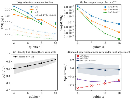
We swept $n\in \{4,6,8,10\}$ and $L\in \{2,3,5\}$ with 50 evaluation tasks and 3 seeds per configuration, recording at ${\theta }_0$ the gradient norms, the alignment A, and after K-step adaptation the local improvement $I_{\mathrm{val}}$ and the query–support gap G; independently, at random initializations, we measured the barren-plateau gradient variance. All correlations are Spearman; methods are in Section 2. Figure 1 summarizes the result.

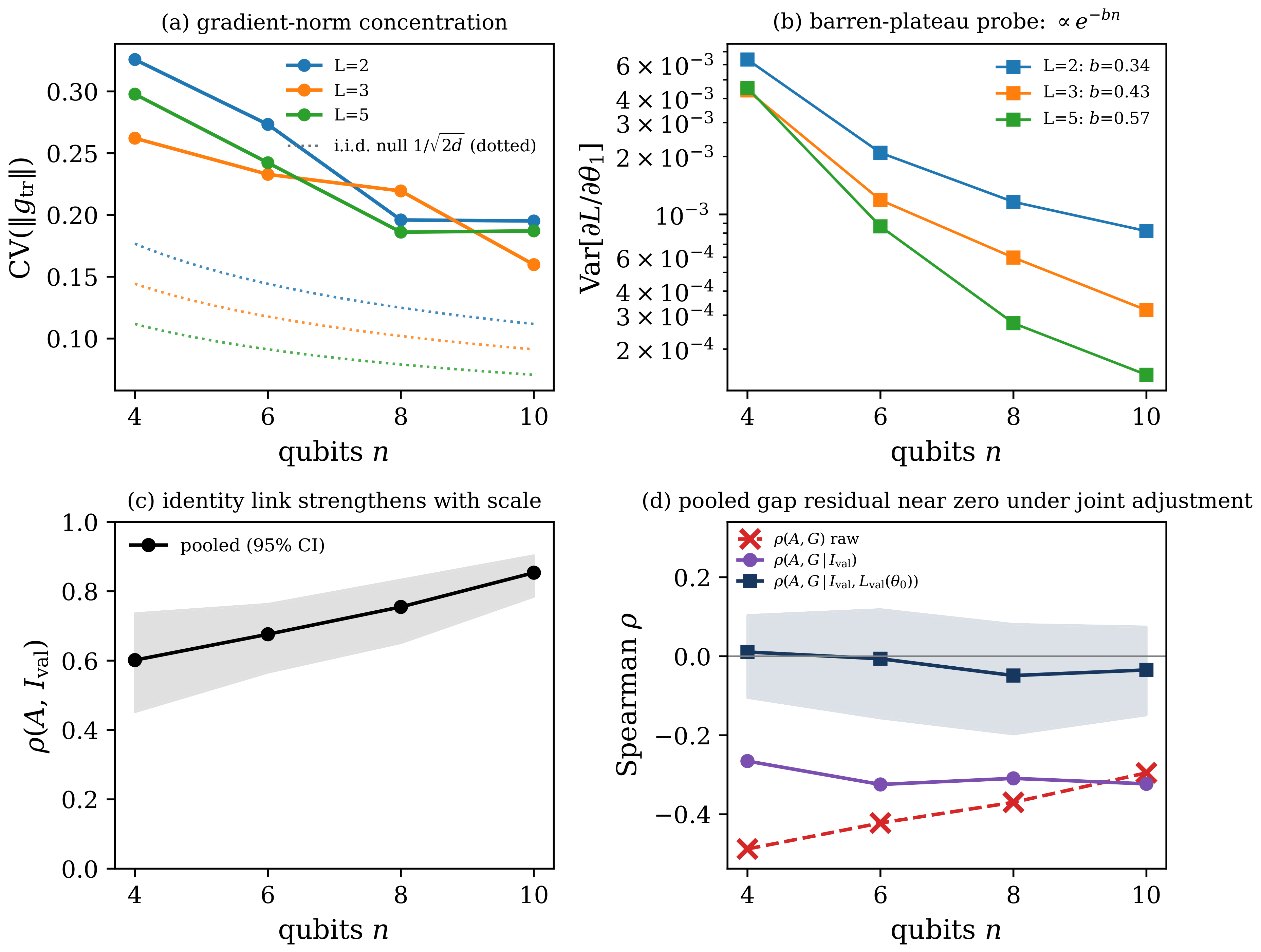
Figure 1. Scale-dependent gradient statistics and alignment behavior across system size ($n=4$–10 qubits, depth $L=2,3,5$; 50 tasks × 3 seeds per point). (a) The gradient-norm coefficient of variation $\mathrm{CV}(\parallel g_{\mathrm{tr}}\parallel )$ concentrates with scale and lies a factor ≈ 2 above the i.i.d. Gaussian dimensional null $1/\sqrt{2d}$ (thin dotted lines, one for each depth in the matching colour), the relative variability exceeds the i.i.d. null, while its decrease with scale parallels the dimensional trend; the directly relevant identity prefactor $q=\parallel g_{\mathrm{tr}}\parallel \parallel g_{\mathrm{val}}\parallel$ concentrates similarly [53]. (b) The barren-plateau probe: the variance of a gradient component at random initialization is consistent with exponential decay, $\propto e^{-bn}$ over the tested range; markers are per-size means connected as a guide to the eye, and b is the exponential-fit rate, increasing with depth ($b=0.34,0.43,0.57$ at $L=2,3,5$). (c) The first-order identity tightens: the pooled rank correlation between alignment A and local validation improvement $I_{\mathrm{val}}$ rises from $\approx 0.60$ at $n=4$ to $\approx 0.85$ at $n=10$ (shaded band: hierarchical-bootstrap $95\%$ CI). (d) The apparent query–support-gap association is accounted for within the specified local-improvement and baseline adjustments: the raw $\rho (A,G)$ (dashed) and the improvement-controlled $\rho (A,G|I_{\mathrm{val}})$ (purple, ≈−0.30) are shown; the pooled residual is near zero after additionally adjusting for the initial validation loss, $\rho (A,G|I_{\mathrm{val}},L_{\mathrm{val}}\left({\theta }_0\right))$ (navy; shaded band: bootstrap $95\%$ CI straddling zero at every size).

Gradients concentrate with scale. The barren-plateau probe [Figure 1b] shows the variance of a single gradient component ($\partial L/\partial {\theta }_1$) decreasing with system size in a way consistent with exponential decay over the tested range ($n\le 10$): a fit $\mathrm{Var}[\partial L/\partial {\theta }_1]\propto e^{-bn}$ gives $b=0.34,0.43,0.57$ per qubit at $L=2,3,5$ (bootstrap $95\%$ CIs of width $\lesssim 0.05$), the rate increasing with depth—a finite-size concentration signature associated with barren-plateau behavior; the mean gradient norm falls in step (from $0.40$ at $n=4$ to $0.18$ at $n=10$). The gradient-norm coefficient of variation [Figure 1a] shows an overall concentration with scale (from $\mathrm{CV}\approx 0.30$ at $n=4$ to ≈0.18–$0.20$ at $n=8$–10), saturating rather than decreasing monotonically at the largest sizes. Importantly, the observed $\mathrm{CV}(\parallel g_{\mathrm{tr}}\parallel )$ exceeds the value expected for an i.i.d. Gaussian gradient of the same dimension $d=2nL$, ${\mathrm{CV}}_{\mathrm{null}}=1/\sqrt{2d}$, by a roughly constant factor ≈ 2 across the sweep; the observed gradients carry larger relative variability than the i.i.d. null, while the decreasing trend itself parallels the dimensional scaling and is not uniquely attributed here. The identity’s prefactor $q=\parallel g_{\mathrm{tr}}\parallel \parallel g_{\mathrm{val}}\parallel$ concentrates in the same way [53]: the pooled $\mathrm{CV}(\parallel g_{\mathrm{val}}\parallel )$ falls from $0.36$ to $0.26$ and $\mathrm{CV}\left(q\right)$ from $0.55$ to ≈0.41–$0.45$ (noisier, as a product of two fluctuating norms), so it is q, not $\parallel g_{\mathrm{tr}}\parallel$ alone, whose relative spread narrows with scale. This is the concentration regime that Equation (3) requires.

The identity tightens with scale. Across the sweep, the alignment–improvement rank correlation rises with system size [Figure 1c], pooled $\rho (A,I_{\mathrm{val}})=0.60,0.68,0.76,0.85$ at $n=4,6,8,10$ (hierarchical-bootstrap $95\%$ CIs $[0.45,0.74]$ and $[0.78,0.90]$ at the endpoints, non-overlapping; consistent across the three seeds), with the identity gap $\rho (⟨g_{\mathrm{tr}},g_{\mathrm{val}}⟩,I_{\mathrm{val}})-\rho (A,I_{\mathrm{val}})\approx 0$ throughout, showing that the cosine and inner-product rankings are similar across this sweep; the attribution analysis (Section 3.5) does not identify CV-based concentration as an independent cause. That the tightening reflects the identity rather than merely a scale-dependent linearization of the K-step trajectory is probed by the one-step limit, where the first-order expression is at its most accurate: with $K=1$ the correlation is $\rho (A,I_{\mathrm{val}}^{\left(1\right)})=0.95,0.96,0.97,0.97$ at $n=4,6,8,10$—already near-perfect and essentially flat in n—whereas the $K=10$ improvement $I_{\mathrm{val}}^{\left(K\right)}$ gives the rising $0.60$–$0.85$ above. The one-step tangent identity is already strong at every size; what scale adds is that the full K-step improvement moves closer to that initial tangent as gradient magnitudes and adaptation steps shrink, while CV-based concentration changes concurrently. Gradient alignment thus reports ever more on the local validation improvement along the support-gradient direction as the circuit is scaled.

The apparent query–support-gap association is sensitive to shared optimization and target-construction quantities. The relationship of alignment to observable generalization requires care [Figure 1d]. The raw $\rho (A,G)$ is moderate and negative and appears to weaken with n ($-0.488,-0.422,-0.370,-0.295$), as do the related $\rho (A,|G\left|\right)$ ($-0.446$ to $-0.208$) and $\rho (A,L_{\mathrm{val}}\left({\theta }_K\right))$ ($-0.557$ to $-0.359$). This weakening is consistent with an algebraic channel shared through the post-adaptation validation loss: G and $I_{\mathrm{val}}$ both contain the post-adaptation validation loss, and their coupling $\rho (I_{\mathrm{val}},G)$ itself shrinks with scale ($-0.507$ to $-0.151$). Controlling for $I_{\mathrm{val}}$ alone leaves a residual that is stable across scale, $\rho (A,G|I_{\mathrm{val}})=-0.27,-0.32,-0.31,-0.32$ ($95\%$ CIs excluding zero). But G is algebraically coupled to a second controlled quantity: through $G=L_{\mathrm{val}}\left({\theta }_K\right)-L_{\mathrm{tr}}\left({\theta }_K\right)$ and $L_{\mathrm{val}}\left({\theta }_K\right)=L_{\mathrm{val}}\left({\theta }_0\right)-I_{\mathrm{val}}$, it carries the initial validation loss $L_{\mathrm{val}}\left({\theta }_0\right)$, which reflects task difficulty at the meta-initialization where A is computed. Controlling for both the local improvement and this baseline yields near-zero pooled residuals at each n: $\rho (A,G|I_{\mathrm{val}},L_{\mathrm{val}}\left({\theta }_0\right))=+0.01,-0.01,-0.05,-0.03$ at $n=4,6,8,10$, with bootstrap CIs straddling zero (e.g., $[-0.14,+0.09]$ at $n=10$). The residual is substantially reduced after adding the initial validation loss to the control set: controlling for $I_{\mathrm{tr}}$ and $I_{\mathrm{val}}$ instead leaves it near $-0.30$, whereas adding $L_{\mathrm{val}}\left({\theta }_0\right)$ yields the near-zero values above; this is a descriptive adjustment result rather than identification of a causal baseline channel.

This baseline dependence can be probed at the level of the target itself. Define the baseline-corrected gap $\Delta G=[L_{\mathrm{val}}\left({\theta }_K\right)-L_{\mathrm{tr}}\left({\theta }_K\right)]-[L_{\mathrm{val}}\left({\theta }_0\right)-L_{\mathrm{tr}}\left({\theta }_0\right)]$, the change in the train–validation gap produced by adaptation, which subtracts the initial baseline by construction. Equivalently $\Delta G=I_{\mathrm{tr}}-I_{\mathrm{val}}$, so this is a check of whether A predicts the adaptation-induced train–validation improvement imbalance beyond its validation-improvement channel. The raw association is again moderate and negative ($\rho (A,\Delta G)=-0.48,-0.55,-0.53,-0.59$), and controlling for the local improvement alone removes it: $\rho (A,\Delta G|I_{\mathrm{val}})=+0.03,-0.03,-0.07,-0.10$ at $n=4,6,8,10$, with bootstrap CIs straddling zero at both endpoints ($[-0.10,+0.15]$ at $n=4$, $[-0.25,+0.07]$ at $n=10$). This is a complementary sensitivity check—the target algebra makes it a statement about the $I_{\mathrm{tr}}$ residual—rather than an independent proof, but it points the same way as the joint control: once the initial baseline is removed from the target, the single control $I_{\mathrm{val}}$ suffices. The same holds for the query loss itself rather than the gap: $\rho (A,L_{\mathrm{val}}\left({\theta }_K\right)|I_{\mathrm{val}},L_{\mathrm{val}}\left({\theta }_0\right))=-0.06,-0.03,-0.10,-0.02$ [53], so the vanishing is not special to the signed gap G.

Two conclusions follow. First, alignment carries no incremental association with the post-adaptation gap beyond the local-improvement and initial-validation-loss channels, within the rank-linear control model used here: its apparent gap signal is accounted for by the local improvement it predicts through the identity and by the initial-loss baseline it shares with G (equivalently, by $I_{\mathrm{val}}$ alone once the baseline is removed from the target). The negative association disappears after adjustment for the initial validation loss; we interpret this descriptively rather than as evidence for a causal baseline mechanism. Second, the identity link strengthens with scale while the (induced) gap association provides no additional pooled rank-linear association after the specified controls (independent out-of-sample utility is not tested here). As circuits grow, the alignment signal is increasingly dominated by its local-improvement component, and gradient alignment is not a stable standalone diagnostic of the same-query-set gap in the tested regime; its out-of-sample transfer utility requires an independent evaluation split.

The setting is a near-zero-mean-transfer regime, by design. It is worth stating plainly what kind of task family this is. Support adaptation improves the support loss substantially (mean $I_{\mathrm{tr}}=+0.41$ down to $+0.16$ across n) but does not improve the query loss on average: the mean validation improvement is $⟨I_{\mathrm{val}}⟩\approx 0$ at every size ($-0.008,+0.002,-0.003,+0.001$), with roughly half of tasks improving and half worsening. This is consistent with the construction: coefficients are drawn independently and, for the linear observable loss over disjoint Pauli sets, no shared minimizer is deliberately imposed; the evaluated task family empirically exhibits little mean observable transfer to detect. Establishing diagnostic behavior in a genuinely positive-transfer family requires a different task construction and an independent evaluation split, which we leave to future work. Rather than weakening the result, this sharpens it: even in a clean setting where genuine mean transfer is absent, the trajectory diagnostics still appear correlated with the query–support gap, and that appearance is accounted for, within the reported rank-linear controls, by the local-improvement and baseline channels above. The quantity the identity predicts is the per-task validation improvement, which retains real spread ($\mathrm{std}\left(I_{\mathrm{val}}\right)=0.28,0.16,0.10,0.06$) even as its mean vanishes. Whether the same diagnostics fail in a genuinely high-transfer regime, which would require a different loss construction, is left to future work.

3.3. Corollary: Adaptation Magnitude Is Decoupled from Observable Generalization

Throughout this subsection, $\mu$ denotes the Reptile meta-initialization parameter vector (the corollary-stage analog of ${\theta }_0$) about which the quadratic drift penalty is taken, and $I_{\mathrm{gap}}\equiv I_{\mathrm{tr}}-I_{\mathrm{val}}$.

The same physics—movement on the variational landscape versus transfer across observables—produces two further failures for the movement-based diagnostics. We report a multi-seed run (denoted v17) of five conditions × three seeds × 50 tasks ($n=150$ per condition) at $n=6$.

First, restraining movement does not improve transfer (Table 2). Across configurations ordered by the observed degree of movement suppression, lower drift co-occurs with higher query-set loss (drift from $0.231$ for plain Reptile down to $0.086$; $L_{\mathrm{val}}$ from $0.506$ up to $0.557$); the five conditions combine different penalty types rather than sweeping a single scalar strength, and plain Reptile, which moves most, attains the lowest query loss. The mean gap G shrinks under strong regularization only because adaptation is suppressed on both sides, co-occurring with the worst $L_{\mathrm{val}}$. Adaptation magnitude on the landscape is thus decoupled from observable generalization.

Table 2. Proximal regularization controls movement but not observable generalization (separate $n=6$ corollary configuration, distinct from the scaling experiment; per-condition means, $n=150$; mean ± std). Across the selected regularization configurations, stronger movement suppression is associated with higher query-set loss.

Condition	Drift	${\mathit{L}}_{\mathbf{val}}$	G
reptile	$0.231\pm 0.039$	$0.506\pm 0.064$	$0.0099$
drift_light	$0.190\pm 0.034$	$0.520\pm 0.063$	$0.0076$
variance_light	$0.227\pm 0.043$	$0.511\pm 0.071$	$0.0090$
full_bqml_light	$0.184\pm 0.036$	$0.525\pm 0.069$	$0.0066$
full_bqml_strong	$0.086\pm 0.019$	$0.557\pm 0.068$	$0.0008$

Second, the movement-based diagnostics inherit this decoupling as predictors (Table 3). Against the pre-specified gap G, drift shows weak and condition-dependent associations: four conditions have $\left|\rho \right|<0.12$ ($p>0.17$), while the strongest regularization condition gives $\rho =+0.227$ ($p=0.005$). In contrast, $V_{\mathrm{tr}}$ remains near zero in all conditions ($\left|\rho \right|<0.034$). The same drift predictor, whose association with G is weak and condition-dependent, is far more strongly associated with support-set improvement $I_{\mathrm{tr}}$ ($\rho \in [0.94,0.99996]$): drift is an adaptation-magnitude diagnostic, not a generalization diagnostic.

Table 3. Movement-based diagnostics primarily track support-set improvement; their associations with the query–support gap are weak and condition-dependent (separate $n=6$ corollary configuration; Spearman, $n=150$ per condition). G is the observable-generalization gap; improvement-based targets are post hoc; $I_{\mathrm{gap}}\equiv I_{\mathrm{tr}}-I_{\mathrm{val}}$.

Condition	Pred.	$\mathit{\rho }\left(\mathit{G}\right)$	p	$\mathit{\rho }\left({\mathit{I}}_{\mathbf{gap}}\right)$	$\mathit{\rho }\left({\mathit{I}}_{\mathbf{tr}}\right)$
reptile	drift	$-0.084$	$0.31$	$0.665$	$0.99989$
drift_light	drift	$-0.107$	$0.19$	$0.621$	$0.99996$
variance_light	drift	$+0.112$	$0.17$	$0.557$	$0.986$
full_bqml_light	drift	$+0.094$	$0.25$	$0.541$	$0.989$
full_bqml_strong	drift	$+0.227$	$0.005$	$0.561$	$0.941$
reptile	$V_{\mathrm{tr}}$	$-0.015$	$0.86$	$0.071$	$0.032$
drift_light	$V_{\mathrm{tr}}$	$-0.033$	$0.69$	$0.031$	$-0.018$
variance_light	$V_{\mathrm{tr}}$	$-0.008$	$0.92$	$0.079$	$0.029$
full_bqml_light	$V_{\mathrm{tr}}$	$-0.025$	$0.76$	$0.026$	$-0.009$
full_bqml_strong	$V_{\mathrm{tr}}$	$-0.026$	$0.76$	$-0.056$	$-0.038$

3.4. Origins of the Movement-Based Signals

The nulls of Section 3.3 coexist with strong correlations against post hoc, improvement-based targets. We trace these to two definitional/physical origins and expose each with a control on the same $n=150$ v17 data.

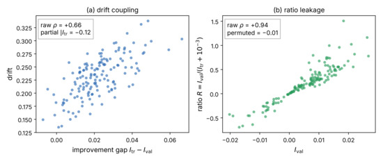
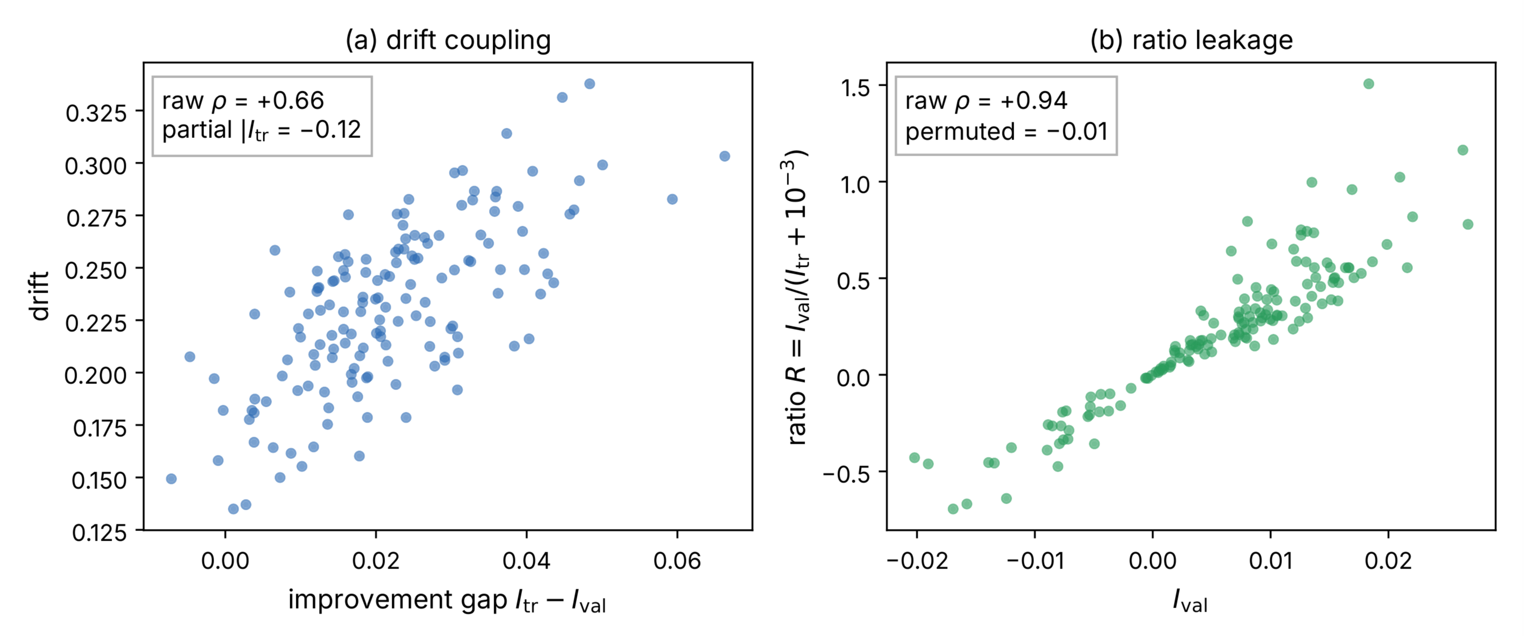
Drift–support-improvement coupling. For gradient-based adaptation, parameter movement is mechanically tied to support-loss reduction, so drift is coupled to $I_{\mathrm{tr}}$ and hence to any target containing $I_{\mathrm{tr}}$ (such as the improvement gap $I_{\mathrm{tr}}-I_{\mathrm{val}}$). The raw drift–improvement-gap correlation is $+0.54$–$0.66$ across conditions, but a partial correlation removing $I_{\mathrm{tr}}$ collapses it to between $-0.34$ and $-0.04$ (reptile $+0.66\to -0.12$; full_bqml_light $+0.54\to -0.34$) [Figure 2a].

Figure 2. Origins of the movement-based signals ($n=6$ v17 run, unregularized condition). (a) Drift’s correlation with the improvement gap ($\rho =+0.66$) collapses after controlling for support improvement (partial $\rho =-0.12$), so the apparent signal is adaptation magnitude, not transfer. (b) A transfer ratio correlates with validation improvement ($\rho =+0.94$), but this is analytic circularity (the target sits in the ratio’s numerator); the target-permutation check ($\rho =-0.01$) illustrates the leaked channel rather than proving it. Spearman correlations per panel.

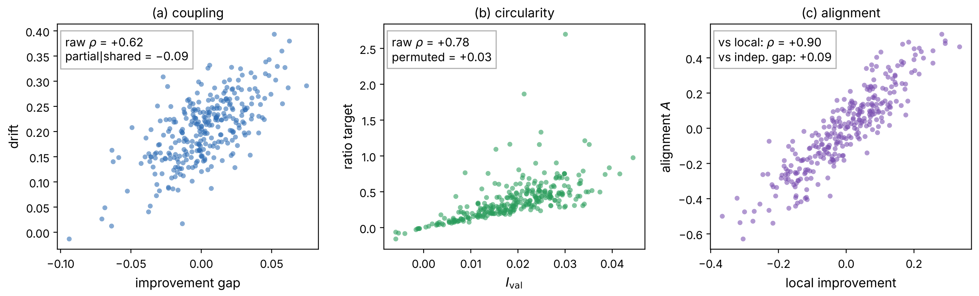
Ratio target leakage. A transfer ratio $R=I_{\mathrm{val}}/(I_{\mathrm{tr}}+ϵ)$ places the target $I_{\mathrm{val}}$ in its own numerator; Figure 2b uses $ϵ={10}^{-3}$, and recomputation from the public per-task data gives $\rho (R,I_{\mathrm{val}})=+0.94$ ($+0.94$–$0.97$ across conditions). Because $I_{\mathrm{val}}$ appears in the numerator, this correlation is circular analytically: the leakage follows from the definition of R, independently of any test, and this algebraic conclusion is independent of the chosen stabilizer value, although the numerical correlation depends on that value. Permuting the target reduces the correlation to $\rho \in [-0.05,+0.15]$; because permutation would also destroy a genuine correlation, this shuffle is a diagnostic illustration of the leaked channel, not the proof of circularity—the proof is definitional [Figure 2b]. A synthetic model isolates both origins in closed form (Figure 3): the coupling correlation collapses under partial control ($+0.62\to -0.09$) and the ratio correlation collapses under target permutation ($+0.78\to +0.03$), while a first-order alignment diagnostic is strong against local improvement ($+0.90$) but near zero against an independently generated gap ($+0.09$), reproducing the metric skeleton that the physical experiments then populate.

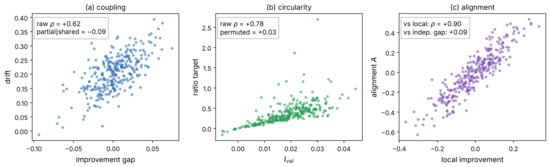
Figure 3. Synthetic isolation of the metric skeleton. (a) Coupling: raw $\rho =+0.62$, partial $\rho =-0.09$ after controlling for the shared component. (b) Circularity: raw $\rho =+0.78$, target-permuted $\rho =+0.03$. (c) A first-order alignment diagnostic is strong against local improvement ($\rho =+0.90$) but near zero against an independently generated gap ($\rho =+0.09$), reproducing the metric skeleton that the physical experiments populate.

3.5. Attribution and Scaling-Form Checks at the Configuration Level

Four post hoc checks on the same per-task data sharpen the scope of the results above; all can be reproduced from the public repository [53].

Heterogeneity beneath the pooled null. The pooled-by-size joint-control residuals reported above coexist with heterogeneity across the 36 $(n,L,\mathrm{seed})$ configurations: per-configuration joint residuals span $-0.17$ to $+0.09$ ($n=4$), $-0.19$ to $+0.15$ ($n=6$), $-0.35$ to $+0.16$ ($n=8$), and $-0.20$ to $+0.17$ ($n=10$), with two $n=8$, $L=5$ seeds nominally significant at $p<0.05$. The pooled statements should therefore be read as pooled statements, not as claims about every configuration.

What the joint-control null does and does not say. Because $G=L_{\mathrm{val}}\left({\theta }_0\right)-I_{\mathrm{val}}-L_{\mathrm{tr}}\left({\theta }_K\right)$ and the joint control set is exactly $\{I_{\mathrm{val}},L_{\mathrm{val}}\left({\theta }_0\right)\}$, linear residualization of G on the controls leaves only the $-L_{\mathrm{tr}}\left({\theta }_K\right)$ component; the rank-based analogue agrees numerically, with $\rho (A,G|I_{\mathrm{val}},L_{\mathrm{val}}\left({\theta }_0\right))$ and $\rho (A,-L_{\mathrm{tr}}\left({\theta }_K\right)|I_{\mathrm{val}},L_{\mathrm{val}}\left({\theta }_0\right))$ differing by at most $0.005$–$0.044$ across sizes. The joint-control null is therefore best read as the statement that alignment carries no additional rank-linear information about the residual training loss, rather than as an independent demonstration that alignment carries no transfer information; distinguishing the latter would require observable splits in which the diagnostic and the evaluation target do not share a measurement set.

Attribution of the identity tightening. At the configuration level, the per-configuration correlation $\rho (A,I_{\mathrm{val}})$ associates with the gradient-norm coefficient of variation (Spearman $-0.44$, $p=8\times {10}^{-3}$), but this association vanishes once the mean gradient norm is partialled out ($+0.18$, $p=0.30$), whereas the mean gradient norm ($-0.75$; $-0.69$ after partialling out the coefficient of variation, $p\approx 3\times {10}^{-6}$) and the mean drift ($-0.70$) retain strong associations. On this dataset, concentration in the coefficient-of-variation sense is therefore not supported as an independent factor; the tightening covaries most strongly with the shrinkage of gradient magnitudes and adaptation trajectories, and disentangling these observationally coupled quantities requires interventional (step-size–matched) experiments beyond the present data.

Scaling form. With four system sizes, the gradient-variance decay is fit comparably by exponential and power-law forms (log-linear versus log–log $R^2$: $0.94$ vs. $0.99$ at $L=2$, $0.97$ vs. $1.00$ at $L=3$, $0.96$ vs. $1.00$ at $L=5$, per-$(n,L)$ means); the exponential fit is used throughout as a finite-range concentration summary, not as an asymptotic scaling classification.

3.6. Independent Split, Task Families with Stronger Transfer, Fixed-Term-Count, and Noise Controls

Four controls added in revision bound the interpretation of the same-query-set audit above; their designs are given in Section 2.2, the pooled statistics are summarized in Table 4, and the full per-seed tables in the Supplementary Material (Tables S8–S12).

Table 4. Revision controls at $L=3$ (pooled over seeds; Spearman $\rho$; per-seed ranges in Tables S8–S11). $A_V$: alignment on the validation terms; $I_V$, $I_T$: validation and unseen-test improvements; $G_T$: out-of-sample gap; joint: rank-partial after adjusting for the improvement and the initial loss of the target subset.

Family	Split, n	Mean ${\mathit{I}}_{\mathit{V}}$	Mean ${\mathit{I}}_{\mathit{T}}$	$\mathit{\rho }({\mathit{A}}_{\mathit{V}},{\mathit{I}}_{\mathit{V}})$	$\mathit{\rho }({\mathit{A}}_{\mathit{V}},{\mathit{I}}_{\mathit{T}})$	Raw $\mathit{\rho }({\mathit{A}}_{\mathit{V}},\mathit{G})$	Joint
original	S–V–T, 6	+0.024	−0.005	+0.66	0.00	+0.02	+0.01
original	S–V–T, 8	+0.007	−0.003	+0.77	−0.10	+0.13	+0.22
correlated	S–V, 6	+0.022	–	+0.68	–	−0.34	−0.12
correlated	S–V–T, 6	+0.005	−0.025	+0.64	+0.06	−0.13	+0.07
uniform	S–V, 6	+0.349	–	+0.15	–	−0.32	−0.11
uniform	S–V–T, 6	+0.277	+0.283	+0.44	−0.06	+0.14	+0.06
uniform	S–V–T, 8	+0.290	+0.278	+0.64	−0.33	+0.10	−0.19

Independent support–validation–test split. When the Pauli terms are partitioned into support, validation, and an unseen test subset, the alignment computed on the validation terms keeps a same-set relation to the validation improvement, $\rho (A_V,I_V)=+0.66$ at $n=6$ and $+0.77$ at $n=8$ (pooled over three seeds), but shows no rank association with the improvement on the test terms, $\rho (A_V,I_T)=0.00$ and $-0.10$ (per-seed ranges $-0.11$ to $+0.13$ and $-0.12$ to $-0.04$). The oracle alignment computed with the test gradient itself does predict $I_T$ ($\rho (A_T,I_T)=+0.63$, $+0.84$), so the first-order relation is a statement about the observables that enter the alignment, and the validation-set alignment carries no detectable out-of-sample content in this family. Against the out-of-sample gap $G_T$ the raw association is $\rho (A_V,G_T)=+0.02$ ($n=6$) and $+0.13$ ($n=8$), and $+0.01$ and $+0.22$ after adjusting for $I_T$ and $L_T\left({\theta }_0\right)$; the positive residual at $n=8$ is consistent with the support-loss term $L_S\left({\theta }_K\right)$ that $G_T$ shares with the adaptation, which the adjustment for the test-subset quantities does not remove.

Task families with stronger observable transfer. The mean validation improvement, $+0.004$ (SE $0.012$) in the original family at $n=6$, is $+0.022$ (SE $0.014$) in the correlated family and $+0.349$ (SE $0.017$) in the uniform family, so the uniform family is a regime with clear positive observable transfer. Under the same two-way split as the main experiment the identity link is $\rho (A,I_{\mathrm{val}})=+0.68$ (correlated) and $+0.15$ (uniform), the raw alignment–gap association is $-0.34$ and $-0.32$, and the jointly adjusted residual is $-0.12$ and $-0.11$ (per-seed ranges $-0.26$ to $-0.09$ and $-0.27$ to $-0.03$). Under the three-way split the validation-set alignment’s association with the unseen-test improvement is $\rho (A_V,I_T)=+0.06$ (correlated, $n=6$), $-0.06$ (uniform, $n=6$), and $-0.33$ (uniform, $n=8$). Transfer therefore does not rescue the diagnostic. Where the observable transfer is large, the validation-set alignment neither predicts the improvement on unseen terms nor retains the same-set identity link that dominates in the null-mean family—improvements of order $0.3$ over ten steps lie well beyond the first-order regime of Equation (3), and even the oracle alignment computed with the test gradient predicts $I_T$ only weakly ($\rho (A_T,I_T)=+0.35$ at $n=6$)—and the jointly adjusted alignment–gap residual in these families is negative rather than near zero, so the near-zero pooled residual of the original family is a property of that regime rather than a general null. The audit’s message, that alignment reports local same-set improvement rather than transfer, holds in both regimes.

Fixed term count. Holding the number of Pauli terms at $M_{\mathrm{fix}}=13$ for all n, the mean support-gradient norm changes from $0.391$ ($n=4$) to $0.308$ ($n=10$), compared with $0.398$ to $0.178$ in the main sweep at $L=3$; the random-initialization variance probe decays from $4.8\times {10}^{-3}$ to $9.6\times {10}^{-4}$; the gradient-norm coefficient of variation is $0.302,0.240,0.212,0.238$ for $n=4,6,8,10$ (main sweep: $0.263,0.239,0.223,0.184$); and the identity link is $\rho (A,I_{\mathrm{val}})=+0.53,+0.65,+0.66,+0.74$ (main sweep: $+0.57,+0.69,+0.83,+0.84$). The term-count control thus separates covariates that the main sweep confounds: the shrinkage of the mean gradient norm with n is largely a term-count and normalization effect and is essentially absent at fixed M, and the coefficient of variation no longer decreases, whereas the decay of the per-component random-initialization variance and the strengthening of the identity link persist at fixed M with reduced magnitude (seeds per size: 2, 2, 1, 1). The scaling statements of Section 3.2 are accordingly read as finite-size trends to which the growing term count contributes, not as evidence of a term-count-independent barren-plateau mechanism.

Depolarizing noise. With single-qubit depolarizing channels after every layer at $n=6$, the mean support-gradient norm is $0.285,0.253,0.171$ for $p=0,0.01,0.05$ (the $p=0$ values are the main-sweep configuration), the identity link is $\rho (A,I_{\mathrm{val}})=+0.69,+0.73,+0.93$, the raw alignment–gap association is $-0.36,-0.32,+0.06$, and the jointly adjusted residual is $+0.00,+0.01,-0.15$. Noise therefore does not weaken the association pattern: it moves the configuration further into the small-gradient regime, the identity link rising as the gradient magnitudes fall, while the raw alignment–gap association shrinks toward zero and the adjusted residual remains small in magnitude ($\left|\rho \right|\le 0.15$); the $p=0.05$ run uses a single seed.

Expressibility. The Kullback–Leibler expressibility of the ansatz [31] is small for every configuration ($D_{\mathrm{KL}}=0.010$–$0.019$ at $n=4$, $0.006$–$0.065$ at $n=6$, $0.001$–$0.032$ at $n=8$, $0.000$–$0.013$ at $n=10$; Table S12), i.e., the fidelity distributions are close to Haar at every tested size and depth, and it decreases with depth within a size. Across the twelve configurations it correlates moderately with the gradient-norm coefficient of variation ($\rho =+0.50$) but not with the identity link ($\rho =+0.10$) or the mean gradient norm ($\rho =+0.04$); within a size, the deeper and more expressive circuits show a weaker identity link ($n=4$: $0.76\to 0.47$; $n=6$: $0.76\to 0.57$; $n=8$: $0.81\to 0.63$; $n=10$: $0.92\to 0.81$ from $L=2$ to $L=5$), in the direction expected from the expressibility–trainability trade-off [30]. Expressibility is therefore reported as a measured covariate: it does not separate the across-size configurations and is not treated as a causal factor.

3.7. An Audit Protocol for Trajectory-Derived Diagnostics

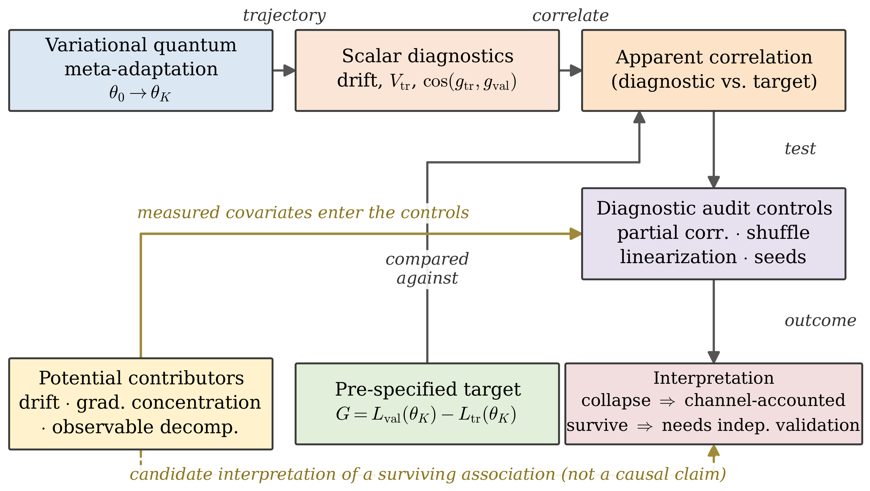
The preceding analyses and their corollaries motivate treating an apparent diagnostic correlation as a candidate association to be stress-tested, not as evidence of observable generalization. We collect the matching controls into a minimal protocol (Table 5; workflow in Figure 4). Beginning from a pre-specified query-set target [Equation (1)]: Control 1 conditions on support improvement (partial correlation removing $I_{\mathrm{tr}}$) to expose drift’s adaptation-magnitude coupling; Control 2 tests the diagnostic against $I_{\mathrm{tr}},I_{\mathrm{val}},G$ separately; Control 3 shuffles the target for ratio metrics to expose circularity; Control 4 checks the linearization identity for alignment ($K=1$ versus $K=10$, prefactor concentration) and, critically, reports the residual under the joint control $\rho (A,G|I_{\mathrm{val}},L_{\mathrm{val}}\left({\theta }_0\right))$—not the $I_{\mathrm{val}}$ control alone, which leaves a baseline-induced residual ($\left|\rho \right|\approx 0.30$ here)—with the baseline-corrected target $\rho (A,\Delta G|I_{\mathrm{val}})$ as an equivalent single-control check, so that the sensitivity of the measured association to local improvement and the initial baseline can be assessed; Control 5 reports signed and absolute gaps; Control 6 requires seed and condition stability; and Control 7 separates diagnostic value from performance improvement (Table 2). The protocol is two-sided: in a synthetic implementation check where an explicit alignment term is added to the target as an implementation check alongside the local-improvement and baseline channels, the association survives the joint control ($\rho =-0.62$, versus $-0.06$ in the channels-only construction) [53], showing that the implemented residualization removes channel-mediated associations while not mechanically forcing an explicitly injected component to zero.

Table 5. Audit protocol for trajectory-derived diagnostics. Each failure mode is paired with the control that exposes it and the trajectory or target-construction feature associated with it.

Failure Mode	Audit Control	Status
Diagnostic–evaluation-set overlap	Independent support–validation–test split (alignment on V, targets on unseen T)	Tested at $n=6,8$ (Section 3.6)
First-order identity (alignment)	$K=1$/$K=10$ check, $\mathrm{CV}\left(q\right)$, $\rho (A,G|I_{\mathrm{val}})$ vs. scale	Demonstrated
Initial-baseline channel	$\rho (A,G|I_{\mathrm{val}},L_{\mathrm{val}}\left({\theta }_0\right))$ and $\rho (A,\Delta G|I_{\mathrm{val}})$	Demonstrated
Support-improvement coupling	Partial correlation controlling $I_{\mathrm{tr}}$	Empirical
Support–query-set conflation	Test $I_{\mathrm{tr}},I_{\mathrm{val}},G$ separately	Empirical
Target leakage (ratio)	Inspect algebraic target overlap; shuffle as illustration	Analytic
Support–query imbalance	Report signed G and $\left|G\right|$	Reported
Seed/condition instability	Report across seeds and conditions	Empirical
Regularization–performance mismatch	Report $L_{\mathrm{val}}$ separately	Empirical

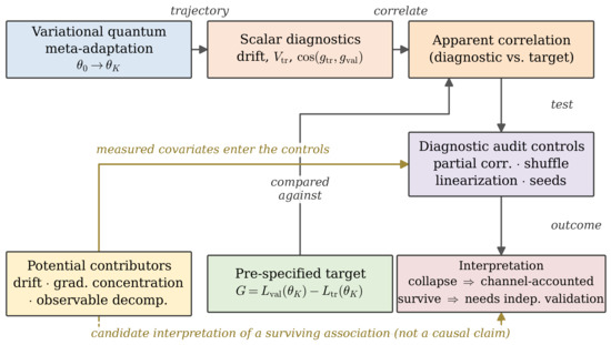
Figure 4. Diagnostic-audit workflow. Trajectory scalars are tested against the pre-specified observable-generalization gap G; apparent correlations with post hoc targets are then subjected to audit controls. The measured covariates (adaptation magnitude, gradient concentration, observable decomposition) enter the controls as control variables (solid arrow) and, for an association that survives, supply candidate interpretations that are not causal claims (dashed connection). Passing the controls does not certify generalization; a collapse identifies dependence on the tested channel but does not establish a unique causal mechanism, and a surviving association still requires independent validation.

4. Discussion

First-order geometry and measured scale-dependent covariates. The through-line of this work is physical: the first-order identity of Equation (3) makes gradient alignment a proxy for the local validation improvement along the support-gradient direction, with a strength that covaries with gradient concentration and with the shrinkage of gradient magnitudes and step displacements; concentration is operationally the same phenomenon that becomes a barren plateau at scale. Sweeping $n=4$–10 and $L=2,3,5$ bears this out: the gradient variance is consistent with exponential decay over the tested range at a depth-increasing rate [Figure 1b], the norm CV decreases with scale while staying above the dimensional null [Figure 1a], and the identity link tightens from $\rho =0.60$ to $0.85$ [Figure 1c]. The practical consequence is of direct interest to VQA practice: as circuits are scaled toward the regime where such diagnostics are most needed, gradient alignment becomes increasingly dominated by local-improvement structure, within the same-query-set design studied here.

The apparent gap signal is accounted for within the specified local-improvement and baseline adjustments. We took care to test whether alignment retains any residual association with the query–support gap. Controlling for the local improvement leaves an apparent residual ($\left|\rho \right|$≈ 0.30), but this is coupled to a second shared quantity: the initial validation-loss baseline $L_{\mathrm{val}}\left({\theta }_0\right)$ that G inherits through the post-adaptation validation loss. For each pooled n, the joint-adjusted residual is near zero; individual depth–seed configurations remain heterogeneous ($\left|\rho \right|\lesssim 0.05$, CIs including zero; Figure 1d), and a sensitivity analysis shows the residual is substantially reduced after adding the initial validation loss to the control set; this is a descriptive adjustment result rather than identification of a causal baseline channel. The negative raw association therefore disappears under baseline adjustment; we read this descriptively rather than as an inverse transfer relation. The honest reading is that alignment’s apparent gap signal is accounted for, within the reported rank-linear controls, by shared local-optimization and baseline quantities, with no incremental association beyond those channels (within the rank-linear control model): as a standalone “higher alignment, better transfer” signal it is misleading, and it becomes increasingly aligned with local-improvement structure as the circuit grows.

Corollaries. In a separate corollary configuration probing the same physical interpretation, movement on the variational landscape is decoupled from observable generalization: proximal regularization suppresses drift while worsening $L_{\mathrm{val}}$ (Table 2), and drift and the variance proxy show weak, condition-dependent associations with G (four conditions $\left|\rho \right|<0.12$; strongest regularization $\rho =0.227$) while drift tracks support improvement almost perfectly (Table 3). These are the movement-based analogs of the alignment result: drift reports on adaptation magnitude, and neither quantity provides a stable standalone transfer diagnostic across the tested conditions.

Robustness checks. Four checks leave the picture intact [53]. First, a term-type-stratified support/query split (balancing $XX,YY,ZZ,Z$ terms across the split so that G cannot be a split artifact) preserves both the identity link ($\rho (A,I_{\mathrm{val}})$ high and rising with n) and the near-zero pooled joint-adjusted association ($\rho (A,G|I_{\mathrm{val}},L_{\mathrm{val}}\left({\theta }_0\right))$ within $\pm 0.05$ at $n=6,8$), matching the uniform split. Second, across two further Hamiltonian families (a transverse-field Ising model and a fixed random-local-Pauli family) and two entangler topologies (linear and ring), the identity link stays high ($\rho (A,I_{\mathrm{val}})=0.49$–$0.91$) and the joint-controlled gap association stays near zero ($-0.17$ to $+0.12$), so the same qualitative association pattern extends beyond the XYZ family and the linear chain. Third, evaluating the variance proxy under a finite shot budget rather than exactly degrades it gracefully: its rank agreement with the exact proxy is $\rho =+0.84$ at 100 shots and $+0.98$ at 1000 shots, with a small positive sampling bias, which shows that finite-shot estimation introduces additional sampling variation and bias. Fourth, replacing the Reptile meta-initialization with a plain random initialization (no meta-training) reproduces the same qualitative association pattern at $n=6$: the identity link is $\rho (A,I_{\mathrm{val}})=+0.74$, the raw gap association is $\rho (A,G)=-0.27$, and it collapses under the joint control to $+0.07$—matching the Reptile arm ($0.68$, $-0.42$, $-0.01$). The same qualitative association pattern is observed under random initialization, indicating that it is not specific to the Reptile meta-initialization.

Relation to prior work. Our study complements capacity- and trainability-level analyses. Caro et al. bound generalization by trainable-gate count [39], with related bounds developed subsequently [41,42,43]; Gil-Fuster et al. show uniform-capacity frameworks fail to explain quantum generalization [44]; and the barren-plateau literature traces gradient concentration to a common algebraic origin [36,37,38] and to overparametrization and noise [54,55], and exponential concentration likewise limits quantum kernel methods [56]. We connect that same finite-size regime to a practical question one level down—what a trajectory diagnostic measures—and report its measured scale-dependent covariates.

What the revision controls add. The independent split answers the question that the same-query-set design cannot. At $n=6$ and 8 the validation-set alignment keeps its same-set relation to the validation improvement but has no rank association with the improvement on unseen test observables ($\rho (A_V,I_T)=0.00$ and $-0.10$), and the same holds in a task family with clear positive transfer (uniform family: mean $I_T=+0.283$ at $n=6$, yet $\rho (A_V,I_T)=-0.06$ and $-0.33$ at $n=6,8$). The first-order identity is thus a statement about the observables that enter the alignment; in these families alignment is a same-set local-improvement report, not an out-of-sample transfer diagnostic, in the null-mean and the positive-transfer regime alike. The transfer-richer families add a second lesson: the identity’s rank dominance is itself regime-dependent, weakening when multi-step improvements are large, so the strong alignment–improvement correlations of the original family should not be extrapolated to transfer-rich settings, where alignment is a weaker same-set predictor and still not an out-of-sample one. The fixed-term-count control qualifies the scaling reading: the shrinkage of the mean gradient norm with size is largely a term-count and normalization effect, while the per-component variance decay and the strengthening of the identity link persist, with reduced magnitude, when the term count is held fixed (Section 3.6). The size dependence of the diagnostics is therefore partly a property of the objective’s construction and partly of the circuit, and we do not attribute it to a barren-plateau mechanism alone. Noise. Depolarizing noise at $n=6$ moves the configuration further into the small-gradient regime: the identity link is +0.69, +0.73, +0.93 for $p=0,0.01,0.05$ while the mean support-gradient norm is 0.285, 0.253, 0.171, the raw alignment–gap association shrinks toward zero, and the adjusted residual stays small in magnitude (Section 3.6). Together with the finite-shot check of the variance proxy (Supplementary Section S5.3; rank correlation $0.84$ at 100 shots and $0.98$ at 1000 shots with the exact value), these runs indicate that the association pattern reported here is not an artifact of noise-free simulation, while shot noise in the gradients themselves and hardware noise beyond the depolarizing model remain open (Limitations). Expressibility, finally, is not the missing covariate: the ansatz is near-Haar at every tested size and depth, and the measure does not separate the configurations across sizes (Section 3.6).

Limitations. The claims are bounded. Term-count confounding: the number of Hamiltonian Pauli terms grows with system size ($M=4n-3$) and the normalized subset losses average over more terms at larger n; the fixed-term-count control (Section 3.6) shows that the shrinkage of the mean gradient norm is largely this term-count effect while the per-component variance decay and the identity strengthening persist with reduced magnitude, but it was run at a single depth with one seed per size at $n=8,10$, so a full fixed-term sweep is left to future work. Scale and breadth: four-to-ten qubits and Reptile as a tractable proxy for second-order meta-learning [57]; the robustness checks above extend to two extra Hamiltonian families and a ring entangler at $n=6$, but a full n-sweep for each family is left to future work, and the gradient-variance decay we observe, while consistent with an exponential form over the tested range and above the dimensional null, is measured below the deep barren-plateau regime. Diagnostic coverage: we tested drift, variance, and alignment; margin-, Fisher/QFIM- [58], and effective-dimension-based [43] measures are not stress-tested here, though the same audit concerns may extend, and diagnostic usefulness is in general task-relative in the spirit of no-free-lunch results for quantum learning [59]. Simulation: the main experiments are noise-free state-vector simulations; the depolarizing-noise control at $n=6$ (Section 3.6) leaves the identity link and the small adjusted residual intact (the identity link strengthens as the gradients shrink), and a finite-shot check confirms the variance proxy degrades gracefully with a positive bias, but shot noise in the gradients and a full noisy-hardware study remain open. Independent split and transfer regime: the three-way split was run at $n=6,8$ and $L=3$ with validation and test subsets of 5–7 terms, and the positive-transfer families at $n=6$ ($n=8$ for one family); the same-query-set analysis remains the primary evidence for the scaling trends, and the split results bound its interpretation rather than replace it. Role of meta-learning: we study the mechanism in a Reptile-style meta-adaptation setting, the natural home for these few-shot trajectory diagnostics, but the random-initialization control (Section 3.2) shows the same qualitative association pattern without Reptile, indicating that it is not specific to the meta-initialization; this comparison does not identify a unique causal mechanism. The identity is first-order and metric-definitional, so it is unlikely to be specific to Reptile, and we have not tested full MAML [57]. The attribution parallels the classical finding that the gains of gradient-based meta-learning stem largely from feature reuse rather than rapid adaptation [20]; the identity supplies the analogous attribution in the variational setting, with measured scale-dependent covariates rather than an isolated mechanism.

5. Conclusions

We audited how first-order geometry, gradient scale, trajectory shrinkage, and target construction shape trajectory-derived diagnostic associations in variational quantum learning. A first-order relation ties support–validation gradient alignment to the local validation improvement along the support-gradient direction. Across $n=4$–10 and $L=2,3,5$, the alignment–improvement correlation increases from $0.60$ to $0.85$ as gradient magnitudes and adaptation trajectories shrink; the present observational analysis does not isolate coefficient-of-variation concentration as an independent cause. The alignment–query–support-gap association is near zero for each pooled system size after the specified joint rank-linear adjustment, while individual depth–seed configurations remain heterogeneous. By target decomposition, this adjusted null is principally a statement about the residual training-loss component and does not establish absence of transfer information. In the separate corollary configuration, drift primarily tracks support improvement and shows weak, condition-dependent gap association, whereas the variance proxy remains near zero against the gap. These findings motivate an audit protocol that identifies dependence on specified optimization and target-construction channels without certifying a unique artifact mechanism. Four controls added in revision bound this reading: under an independent support–validation–test split the validation-set alignment has no rank association with the improvement on unseen observables at $n=6,8$ ($\rho =0.00$, $-0.10$), including in a task family with clear positive transfer; with the Pauli-term count held fixed, the shrinkage of the mean gradient norm largely disappears while the per-component variance decay and the strengthening of the identity link persist with reduced magnitude; depolarizing noise at $n=6$ strengthens rather than weakens the identity link and leaves the adjusted residual small; and the ansatz is near-Haar expressible at every tested size and depth, so expressibility does not separate the configurations. The primary scaling analysis remains a same-query-set, noise-free study at $n\le 10$, and the controls were run at $L=3$, with the split and family controls at $n\le 8$, the fixed-term control at $n\le 10$, and noise at $n=6$. Natural extensions are to push toward the deep barren-plateau regime with larger systems and other ansatz templates, to independent-split sweeps across depths and families, to literature diagnostics (margin, Fisher/QFIM, effective dimension), and to hardware data, where finite-shot statistics enter the variance proxy directly.

References

- Cerezo, M.; Arrasmith, A.; Babbush, R.; Benjamin, S.C.; Endo, S.; Fujii, K.; McClean, J.R.; Mitarai, K.; Yuan, X.; Cincio, L.; et al. Variational quantum algorithms. Nat. Rev. Phys. 2021, 3, 625. [Google Scholar] [CrossRef] [Scilit]
- Bharti, K.; Cervera-Lierta, A.; Kyaw, T.H.; Haug, T.; Alperin-Lea, S.; Anand, A.; Degroote, M.; Heimonen, H.; Kottmann, J.S.; Menke, T.; et al. Noisy intermediate-scale quantum algorithms. Rev. Mod. Phys. 2022, 94, 015004. [Google Scholar] [CrossRef] [Scilit]
- Biamonte, J.; Wittek, P.; Pancotti, N.; Rebentrost, P.; Wiebe, N.; Lloyd, S. Quantum machine learning. Nature 2017, 549, 195. [Google Scholar] [CrossRef] [Scilit] [PubMed]
- Benedetti, M.; Lloyd, E.; Sack, S.; Fiorentini, M. Parameterized quantum circuits as machine learning models. Quantum Sci. Technol. 2019, 4, 043001, Correction in Quantum Sci. Technol. 2020, 5, 019601. https://doi.org/10.1088/2058-9565/ab5944. [Google Scholar] [CrossRef] [Scilit]
- Havlíček, V.; Córcoles, A.D.; Temme, K.; Harrow, A.W.; Kandala, A.; Chow, J.M.; Gambetta, J.M. Supervised learning with quantum-enhanced feature spaces. Nature 2019, 567, 209. [Google Scholar] [CrossRef] [Scilit] [PubMed]
- Schuld, M.; Killoran, N. Quantum machine learning in feature Hilbert spaces. Phys. Rev. Lett. 2019, 122, 040504. [Google Scholar] [CrossRef] [Scilit] [PubMed]
- Schuld, M.; Sweke, R.; Meyer, J.J. Effect of data encoding on the expressive power of variational quantum-machine-learning models. Phys. Rev. A 2021, 103, 032430. [Google Scholar] [CrossRef] [Scilit]
- Du, Y.; Tu, Z.; Yuan, X.; Tao, D. Efficient measure for the expressivity of variational quantum algorithms. Phys. Rev. Lett. 2022, 128, 080506. [Google Scholar] [CrossRef] [Scilit] [PubMed]
- Mitarai, K.; Negoro, M.; Kitagawa, M.; Fujii, K. Quantum circuit learning. Phys. Rev. A 2018, 98, 032309. [Google Scholar] [CrossRef] [Scilit]
- Schuld, M.; Bergholm, V.; Gogolin, C.; Izaac, J.; Killoran, N. Evaluating analytic gradients on quantum hardware. Phys. Rev. A 2019, 99, 032331. [Google Scholar] [CrossRef] [Scilit]
- McClean, J.R.; Romero, J.; Babbush, R.; Aspuru-Guzik, A. The theory of variational hybrid quantum-classical algorithms. New J. Phys. 2016, 18, 023023. [Google Scholar] [CrossRef] [Scilit]
- Peruzzo, A.; McClean, J.; Shadbolt, P.; Yung, M.-H.; Zhou, X.-Q.; Love, P.J.; Aspuru-Guzik, A.; O’Brien, J.L. A variational eigenvalue solver on a photonic quantum processor. Nat. Commun. 2014, 5, 4213. [Google Scholar] [CrossRef] [Scilit] [PubMed]
- Preskill, J. Quantum computing in the NISQ era and beyond. Quantum 2018, 2, 79. [Google Scholar] [CrossRef] [Scilit]
- Jiang, Y.; Neyshabur, B.; Mobahi, H.; Krishnan, D.; Bengio, S. Fantastic generalization measures and where to find them. arXiv 2020, arXiv:1912.02178. [Google Scholar]
- Keskar, N.S.; Mudigere, D.; Nocedal, J.; Smelyanskiy, M.; Tang, P.T.P. On large-batch training for deep learning: Generalization gap and sharp minima. arXiv 2017, arXiv:1609.04836. [Google Scholar]
- Dziugaite, G.K.; Roy, D.M. Computing nonvacuous generalization bounds for deep (stochastic) neural networks with many more parameters than training data. arXiv 2017, arXiv:1703.11008. [Google Scholar]
- Hochreiter, S.; Schmidhuber, J. Flat minima. Neural Comput. 1997, 9, 1. [Google Scholar] [CrossRef] [Scilit] [PubMed]
- Dziugaite, G.K.; Drouin, A.; Neal, B.; Rajkumar, N.; Caballero, E.; Wang, L.; Mitliagkas, I.; Roy, D.M. In search of robust measures of generalization. arXiv 2020, arXiv:2010.11924. [Google Scholar]
- Hospedales, T.M.; Antoniou, A.; Micaelli, P.; Storkey, A.J. Meta-learning in neural networks: A survey. IEEE Trans. Pattern Anal. Mach. Intell. 2022, 44, 5149. [Google Scholar] [CrossRef] [Scilit] [PubMed]
- Raghu, A.; Raghu, M.; Bengio, S.; Vinyals, O. Rapid learning or feature reuse? Towards understanding the effectiveness of MAML. arXiv 2020, arXiv:1909.09157. [Google Scholar]
- Yin, M.; Tucker, G.; Zhou, M.; Levine, S.; Finn, C. Meta-learning without memorization. arXiv 2020, arXiv:1912.03820. [Google Scholar]
- Chen, W.-Y.; Liu, Y.-C.; Kira, Z.; Wang, Y.-C.F.; Huang, J.-B. A closer look at few-shot classification. arXiv 2019, arXiv:1904.04232. [Google Scholar]
- Dhillon, G.S.; Chaudhari, P.; Ravichandran, A.; Soatto, S. A baseline for few-shot image classification. arXiv 2020, arXiv:1909.02729. [Google Scholar]
- Wilson, M.; Stromswold, R.; Wudarski, F.; Hadfield, S.; Tubman, N.M.; Rieffel, E.G. Optimizing quantum heuristics with meta-learning. Quantum Mach. Intell. 2021, 3, 13. [Google Scholar] [CrossRef] [Scilit]
- Huang, R.; Tan, X.; Xu, Q. Learning to learn variational quantum algorithm. IEEE Trans. Neural Netw. Learn. Syst. 2023, 34, 8430–8440. [Google Scholar] [CrossRef] [Scilit] [PubMed]
- Chandarana, P.; Vieites, P.S.; Hegade, N.N.; Solano, E.; Ban, Y.; Chen, X. Meta-learning digitized-counterdiabatic quantum optimization. Quantum Sci. Technol. 2023, 8, 045007. [Google Scholar] [CrossRef] [Scilit]
- Lee, J.; Cho, J.; Kim, S. Q-MAML: Quantum model-agnostic meta-learning for variational quantum algorithms. Proc. AAAI Conf. Artif. Intell. 2025, 39, 18137–18144. [Google Scholar] [CrossRef] [Scilit]
- McClean, J.R.; Boixo, S.; Smelyanskiy, V.N.; Babbush, R.; Neven, H. Barren plateaus in quantum neural network training landscapes. Nat. Commun. 2018, 9, 4812. [Google Scholar] [CrossRef] [Scilit] [PubMed]
- Cerezo, M.; Sone, A.; Volkoff, T.; Cincio, L.; Coles, P.J. Cost function dependent barren plateaus in shallow parametrized quantum circuits. Nat. Commun. 2021, 12, 1791. [Google Scholar] [CrossRef] [Scilit] [PubMed]
- Holmes, Z.; Sharma, K.; Cerezo, M.; Coles, P.J. Connecting ansatz expressibility to gradient magnitudes and barren plateaus. PRX Quantum 2022, 3, 010313. [Google Scholar] [CrossRef] [Scilit]
- Sim, S.; Johnson, P.D.; Aspuru-Guzik, A. Expressibility and entangling capability of parameterized quantum circuits for hybrid quantum-classical algorithms. Adv. Quantum Technol. 2019, 2, 1900070. [Google Scholar] [CrossRef] [Scilit]
- Wang, S.; Fontana, E.; Cerezo, M.; Sharma, K.; Sone, A.; Cincio, L.; Coles, P.J. Noise-induced barren plateaus in variational quantum algorithms. Nat. Commun. 2021, 12, 6961. [Google Scholar] [CrossRef] [Scilit] [PubMed]
- Marrero, C.O.; Kieferóvá, M.; Wiebe, N. Entanglement-induced barren plateaus. PRX Quantum 2021, 2, 040316. [Google Scholar] [CrossRef] [Scilit]
- Cerezo, M.; Coles, P.J. Higher order derivatives of quantum neural networks with barren plateaus. Quantum Sci. Technol. 2021, 6, 035006. [Google Scholar] [CrossRef] [Scilit]
- Arrasmith, A.; Cerezo, M.; Czarnik, P.; Cincio, L.; Coles, P.J. Effect of barren plateaus on gradient-free optimization. Quantum 2021, 5, 558. [Google Scholar] [CrossRef] [Scilit]
- Ragone, M.; Bakalov, B.N.; Sauvage, F.; Kemper, A.F.; Marrero, C.O.; Larocca, M.; Cerezo, M. A Lie algebraic theory of barren plateaus for deep parameterized quantum circuits. Nat. Commun. 2024, 15, 7172. [Google Scholar] [CrossRef] [Scilit] [PubMed]
- Fontana, E.; Herman, D.; Chakrabarti, S.; Kumar, N.; Yalovetzky, R.; Heredge, J.; Sureshbabu, S.H.; Pistoia, M. Characterizing barren plateaus in quantum ansätze with the adjoint representation. Nat. Commun. 2024, 15, 7171. [Google Scholar] [CrossRef] [Scilit] [PubMed]
- Larocca, M.; Thanasilp, S.; Wang, S.; Sharma, K.; Biamonte, J.; Coles, P.J.; Cincio, L.; McClean, J.R.; Holmes, Z.; Cerezo, M. Barren plateaus in variational quantum computing. Nat. Rev. Phys. 2025, 7, 174. [Google Scholar] [CrossRef] [Scilit]
- Caro, M.C.; Huang, H.-Y.; Cerezo, M.; Sharma, K.; Sornborger, A.; Cincio, L.; Coles, P.J. Generalization in quantum machine learning from few training data. Nat. Commun. 2022, 13, 4919. [Google Scholar] [CrossRef] [Scilit] [PubMed]
- Caro, M.C.; Huang, H.-Y.; Ezzell, N.; Gibbs, J.; Sornborger, A.T.; Cincio, L.; Coles, P.J.; Holmes, Z. Out-of-distribution generalization for learning quantum dynamics. Nat. Commun. 2023, 14, 3751. [Google Scholar] [CrossRef] [Scilit] [PubMed]
- Caro, M.C.; Gil-Fuster, E.; Meyer, J.J.; Eisert, J.; Sweke, R. Encoding-dependent generalization bounds for parametrized quantum circuits. Quantum 2021, 5, 582. [Google Scholar] [CrossRef] [Scilit]
- Banchi, L.; Pereira, J.; Pirandola, S. Generalization in quantum machine learning: A quantum information standpoint. PRX Quantum 2021, 2, 040321. [Google Scholar] [CrossRef] [Scilit]
- Abbas, A.; Sutter, D.; Zoufal, C.; Lucchi, A.; Figalli, A.; Woerner, S. The power of quantum neural networks. Nat. Comput. Sci. 2021, 1, 403. [Google Scholar] [CrossRef] [Scilit] [PubMed]
- Gil-Fuster, E.; Eisert, J.; Bravo-Prieto, C. Understanding quantum machine learning also requires rethinking generalization. Nat. Commun. 2024, 15, 2277. [Google Scholar] [CrossRef] [Scilit] [PubMed]
- Peters, E.; Schuld, M. Generalization despite overfitting in quantum machine learning models. Quantum 2023, 7, 1210. [Google Scholar] [CrossRef] [Scilit]
- Nichol, A.; Achiam, J.; Schulman, J. On first-order meta-learning algorithms. arXiv 2018, arXiv:1803.02999. [Google Scholar]
- Verdon, G.; Broughton, M.; McClean, J.R.; Sung, K.J.; Babbush, R.; Jiang, Z.; Neven, H.; Mohseni, M. Learning to learn with quantum neural networks via classical neural networks. arXiv 2019, arXiv:1907.05415. [Google Scholar]
- Cervera-Lierta, A.; Kottmann, J.S.; Aspuru-Guzik, A. The meta-variational quantum eigensolver: Learning energy profiles of parameterized Hamiltonians for quantum simulation. PRX Quantum 2021, 2, 020329. [Google Scholar] [CrossRef] [Scilit]
- Puig, R.; Drudis, M.; Thanasilp, S.; Holmes, Z. Variational quantum simulation: A case study for understanding warm starts. PRX Quantum 2025, 6, 010317. [Google Scholar] [CrossRef] [Scilit]
- Grant, E.; Wossnig, L.; Ostaszewski, M.; Benedetti, M. An initialization strategy for addressing barren plateaus in parametrized quantum circuits. Quantum 2019, 3, 214. [Google Scholar] [CrossRef] [Scilit]
- Skolik, A.; McClean, J.R.; Mohseni, M.; Smagt, P.v.; Leib, M. Layerwise learning for quantum neural networks. Quantum Mach. Intell. 2021, 3, 5. [Google Scholar] [CrossRef] [Scilit]
- Huang, H.-Y.; Kueng, R.; Preskill, J. Predicting many properties of a quantum system from very few measurements. Nat. Phys. 2020, 16, 1050. [Google Scholar] [CrossRef] [Scilit]
- Oh, S.H. Data and Supplementary Material for This Article. 2026. Available online: https://github.com/shoh0320/qml-trajectory-diagnostics (accessed on 17 September 2026).
- Larocca, M.; Ju, N.; García-Martín, D.; Coles, P.J.; Cerezo, M. Theory of overparametrization in quantum neural networks. Nat. Comput. Sci. 2023, 3, 542. [Google Scholar] [CrossRef] [Scilit] [PubMed]
- García-Martín, D.; Larocca, M.; Cerezo, M. Effects of noise on the overparametrization of quantum neural networks. Phys. Rev. Res. 2024, 6, 013295. [Google Scholar] [CrossRef] [Scilit]
- Thanasilp, S.; Wang, S.; Cerezo, M.; Holmes, Z. Exponential concentration in quantum kernel methods. Nat. Commun. 2024, 15, 5200. [Google Scholar] [CrossRef] [Scilit] [PubMed]
- Finn, C.; Abbeel, P.; Levine, S. Model-agnostic meta-learning for fast adaptation of deep networks. arXiv 2017, arXiv:1703.03400. [Google Scholar]
- Haug, T.; Kim, M.S. Generalization of quantum machine learning models using quantum Fisher information metric. Phys. Rev. Lett. 2024, 133, 050603. [Google Scholar] [CrossRef] [Scilit] [PubMed]
- Sharma, K.; Cerezo, M.; Holmes, Z.; Cincio, L.; Sornborger, A.; Coles, P.J. Reformulation of the no-free-lunch theorem for entangled datasets. Phys. Rev. Lett. 2022, 128, 070501. [Google Scholar] [CrossRef] [Scilit] [PubMed]
Disclaimer/Publisher’s Note: The statements, opinions and data contained in all publications are solely those of the individual author(s) and contributor(s) and not of MDPI and/or the editor(s). MDPI and/or the editor(s) disclaim responsibility for any injury to people or property resulting from any ideas, methods, instructions or products referred to in the content. |
© 2026 by the author. Licensee MDPI, Basel, Switzerland. This article is an open access article distributed under the terms and conditions of the Creative Commons Attribution (CC BY) license.