A Triple Compensation Method for Correcting Temperature-Induced Distance Errors in SPAD-Based d-ToF LiDAR

Abstract

This paper proposes a Triple Compensation Method to systematically eliminate thermal degradation and distance measurement errors induced by temperature variations in SPAD (Single-Photon Avalanche Diode)-based direct Time-of-Flight (d-ToF) LiDAR sensors. As temperature rises, the combined effects of reduced emission efficiency in the transmitter’s Laser Diode (LD) and an increase in the breakdown voltage (V_BD) of the receiver’s SPAD element result in decreased peak intensity and pulse width distortion. These factors directly cause rising-edge timing distortions, introducing significant walk errors and thermal distance drift. The proposed triple compensation scheme comprises three distinct stages: 1. Track 1 (Dynamic Gain Control): Real-time monitoring of junction temperature dynamically adjusts the bias voltage (V_Bias) to maintain constant excess voltage (V_Ex), mitigating degradations in Photon Detection Efficiency (PDE) and gain. 2. Track 2 (Walk Error Compensation): Residual non-linear walk errors are corrected by real-time tracking of peak intensity using an empirically derived look-up table (LUT). 3. Track 3 (Unit-Specific LUT Compensation): Circuit delay drifts caused by manufacturing process variations are compensated by applying a unit-specific calibration curve, derived via 3-sigma filtering and second-order polynomial fitting (R2 = 0.991), stored in non-volatile memory (NVM). Experimental validation across a temperature range of −20 °C to 60 °C demonstrates that the proposed triple compensation reduces the peak-to-peak distance error from 1.11 m to 0.16 m (an 85.6% reduction) and decreases the standard deviation from 0.30 m to 0.035 m (an 88.3% reduction), achieving an 8.57-fold improvement in precision. This approach offers a highly practical and scalable solution for high-precision LiDAR operation without requiring costly physical cooling hardware.

1. Introduction

1.1. Background

With the rapid growth of the autonomous vehicle and unmanned vehicle industries, there is increasing demand for direct Time-of-Flight (d-ToF) based LiDAR technology as a core sensor for precisely perceiving the surrounding environment. In particular, SPAD d-ToF LiDAR, which adopts a Single-Photon Avalanche Diode (SPAD) as a receiver, possesses high sensitivity and excellent temporal resolution capable of detecting even minute signals at the single-photon level. Through this, it demonstrates excellent performance in long-range measurement and low-reflectivity object detection, and is receiving significant attention as a next-generation high-performance perception sensor [1,2,3].

However, SPAD-based d-ToF LiDARs undergo complex thermal degradation throughout the transmitter and receiver when exposed to rapid temperature changes in outdoor driving environments [4].

• Transmission side: As the temperature of the laser diode (LD) increases, non-radiative recombination within the active layer increases and the threshold current rises, resulting in a decrease in photoluminescence efficiency relative to the same driving current. This leads to a reduction in the peak output of the transmitted pulse and waveform distortion.
• Receiver side: Increased semiconductor lattice oscillation (phonon scattering) causes the breakdown voltage (V_BD) of the SPAD device to rise. As a result, under fixed bias voltage (V_Bias) conditions, the excess voltage (V_Ex = V_Bias − V_BD) decreases, which leads to a simultaneous decrease in Photon Detection Efficiency (PDE) and Gain.

1.2. Limitations of Existing Works

Existing thermal compensation techniques in d-ToF LiDAR generally fall into two categories: hardware-level active stabilization and software-level algorithmic corrections. Hardware approaches, such as thermoelectric coolers (TECs) or active voltage tracking loops, provide direct compensation but introduce significant power overhead and hardware complexity [5,6,7,8,9]. Conversely, software-driven approaches utilize look-up tables (LUTs) or analytical drift functions, offering lightweight solutions but often failing to account for non-linear dynamic walk errors. To address these limitations, this work proposes a hybrid architecture that synergizes hardware-assisted bias regulation with software-based walk error and polynomial calibrations.

1.3. Objectives

This study proposes a Triple Compensation technique based on the physical mechanisms of error causes without the need for a separate physical cooling device, aiming to precisely compensate for the temperature-dependent distance measurement error of SPAD d-ToF LiDAR.

The proposed Triple Compensation technique operates in a three-stage system as follows, tailored to physical error factors:

• Track 1 (Dynamic Gain Control, GC): By monitoring the junction temperature of the SPAD in real time and dynamically controlling V_Bias, V_Ex is maintained at a constant level. This preserves the receive gain and PDE, thereby primarily suppressing peak intensity degradation and pulse width distortion.
• Track 2 (Walk Error Compensation): It tracks non-linear fluctuations in received peak intensity remaining after GC application in real time and applies a Walk Error LUT for each peak intensity derived from light intensity control measurement experiments to provide secondary compensation for rising edge timing delay.
• Track 3 (Unit-Specific Calibration LUT): During the production calibration stage, 3-sigma preprocessing and 2nd-order polynomial fitting are performed to compensate for the unit’s temperature-dependent delay drift caused by circuit element and process deviations in a 2nd order, and this is stored in NVM (Non-Volatile Memory).

This paper quantitatively identifies the physical correlation between peak intensity, pulse width, and rising edge delay characteristics according to temperature through the analysis of actual waveform data and experimentally verifies that distance measurement accuracy is improved by more than 10 times in a wide temperature range of −20 °C to 60 °C by applying the proposed triple compensation stepwise.

1.4. Nomenclature and Notation Standardization

To ensure mathematical consistency and clarity throughout the manuscript, all physical parameters, supply voltages, and hardware channel designations have been unified. Table 1 summarizes the standardized nomenclature applied across all equations, figures, tables, and narrative text.

Table 1. Standardized nomenclature and notation used throughout the manuscript.

Parameter/Term	Standardized Notation	Description	Superseded/Deprecated Terms
Excess Voltage	VEx	Applied voltage above the breakdown threshold (Vbias − VBD)	Vexcess, Vex, Excess voltage
Breakdown Voltage	VBD	Voltage threshold at which avalanche breakdown occurs in SPAD	Vbr, Vbreakdown
Normal Channel	Normal Channel	Receiver channel exposed to incident laser photons for ranging	Active Channel, Main Channel, Signal Channel
Dark Channel	Dark Channel	Receiver channel optically masked from target photons for thermal monitoring	Blind Channel, Dummy Channel, Masked Channel
Peak Intensity	Peak Intensity (LSB)	Digitized peak amplitude of received histogram signal in LSB units	Signal Power, Peak LSB, Amplitude, Intensity Count

2. Materials and Methods

2.1. Theoretical Background and Thermal Drift Mechanisms

2.1.1. Operating Principle of d-ToF LiDAR

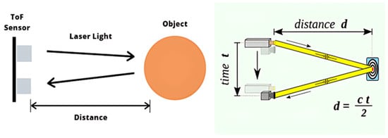
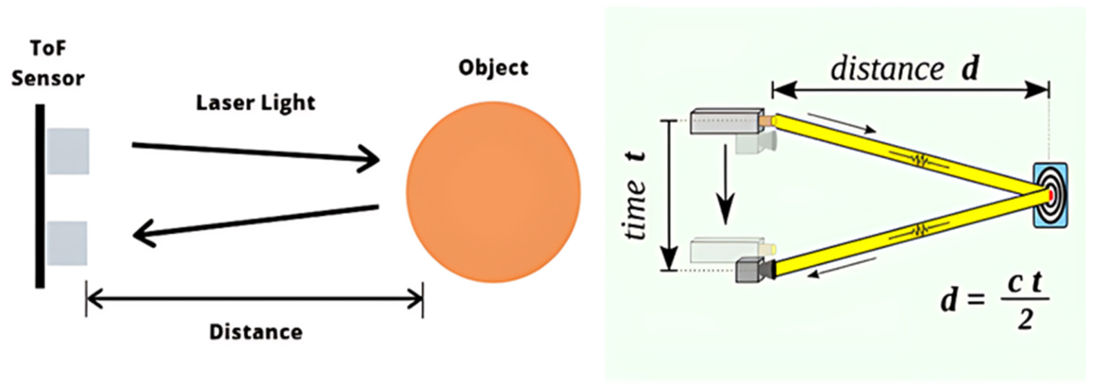
The direct Time-of-Flight (d-ToF) operating principle relies on measuring the total elapsed round-trip time (Δt) between the emission of a short laser pulse and its detection by the receiver. As conceptually illustrated in Figure 1, the measured distance d is mathematically expressed as:

$$d={\displaystyle \frac{c\cdot \Delta t}{2}}$$

(1)

where c represents the speed of light in air.

Figure 1. Operational principle of direct Time-of-Flight (d-ToF) LiDAR distance measurement based on the laser pulse round-trip time.

In a SPAD-based receiver operating in Geiger mode, the single-photon avalanche diode is reverse-biased at a voltage V_Bias higher than its breakdown voltage V_BD. A key physical parameter governing the receiver performance is the excess voltage V_Ex, defined as:

V_Ex = V_Bias − V_BD

(2)

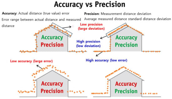
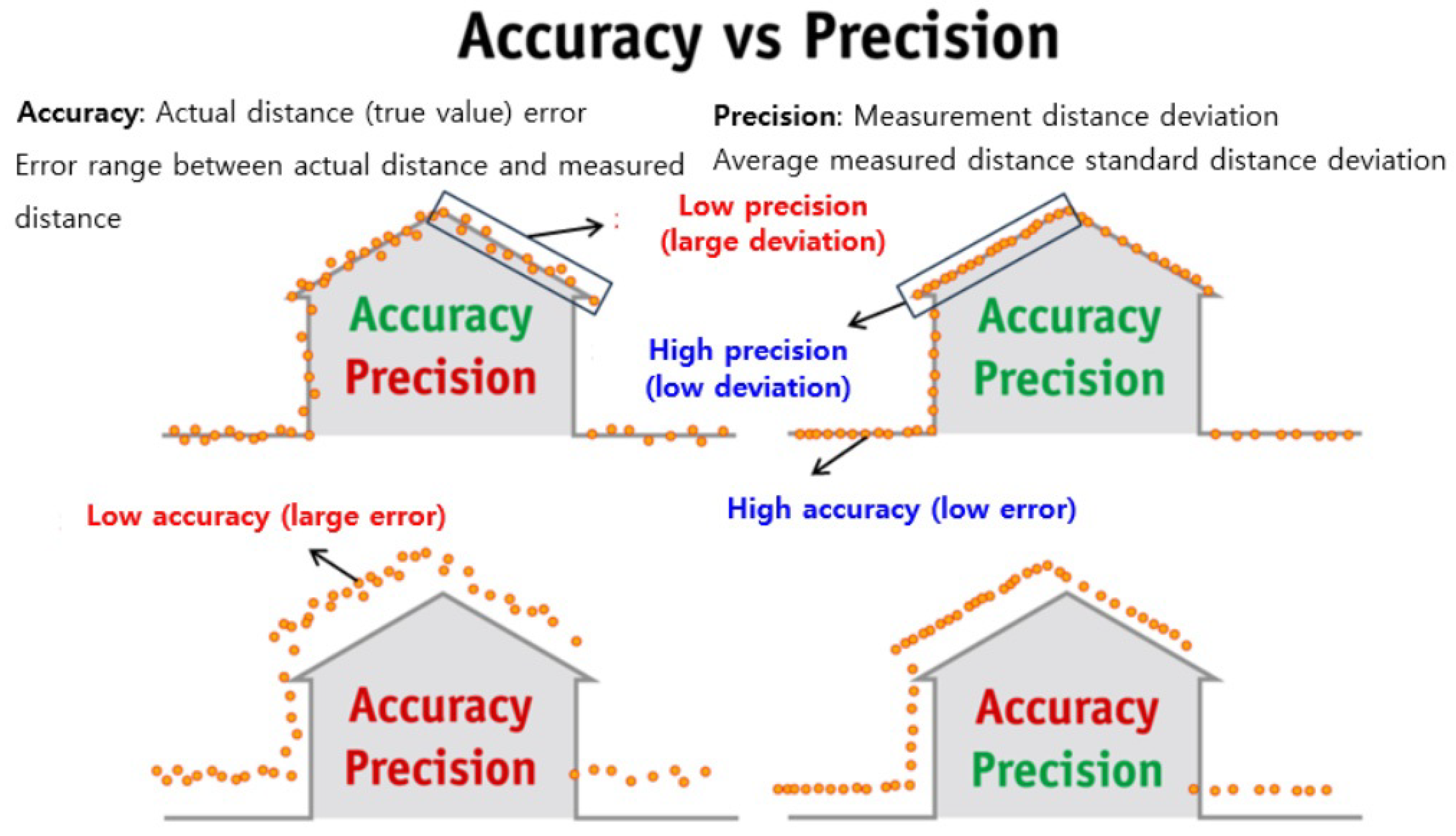
Excess voltage directly dictates two fundamental physical characteristics of the SPAD element: Photon Detection Efficiency (PDE), which determines photon absorption and avalanche probability, and internal multiplication gain, which governs the digitized peak signal amplitude. Figure 2 clarifies the fundamental distinction between systematic ranging accuracy (mean error from true distance) and statistical precision (standard deviation, σ) affected by these parameters under thermal fluctuations.

Figure 2. Conceptual distinction between distance accuracy (systematic error from true distance) and measurement precision (repeatability and standard deviation of measured points).

2.1.2. Transmitter Optical Degradation (Laser Diode Shift)

When exposed to ambient thermal variations, the transmitter module suffers from significant optical degradation. As the junction temperature (T_j) of the Laser Diode (LD) rises, non-radiative recombination within the active layer increases, causing the threshold current to rise and reducing the overall photoluminescence efficiency.

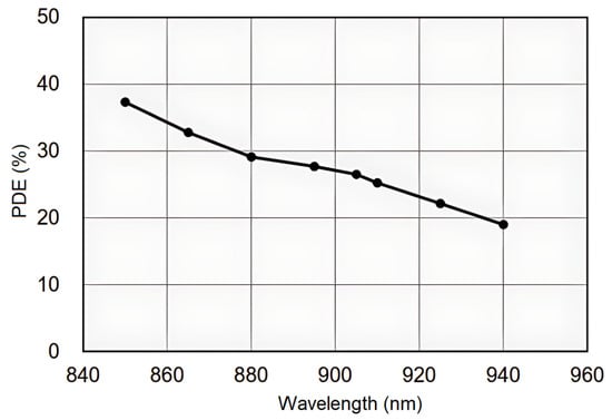
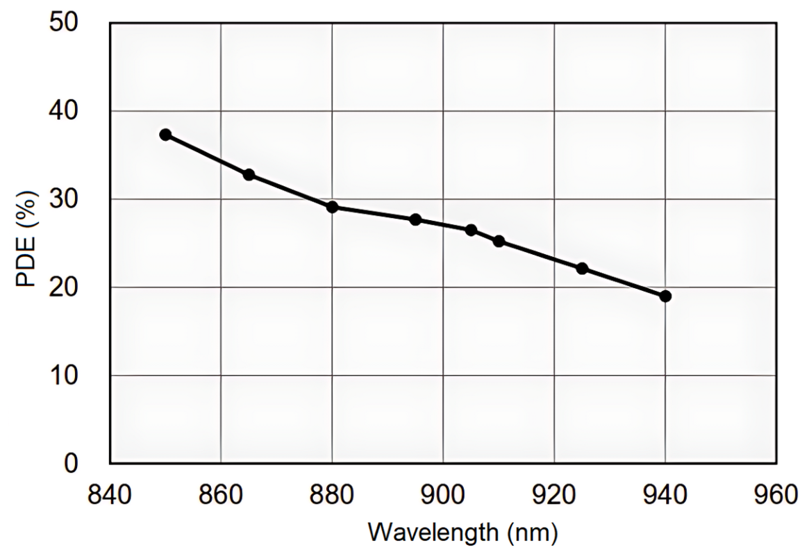
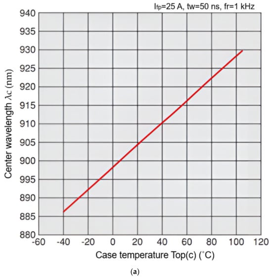
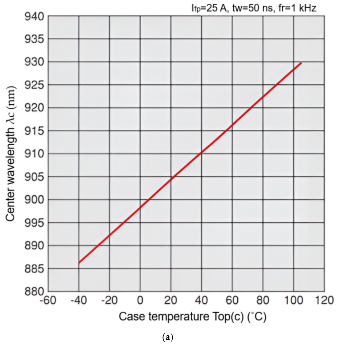
Concurrently, as shown in Figure 3, silicon-based photodetectors exhibit lower PDE at longer wavelengths in the near-infrared spectrum. Furthermore, as depicted in Figure 4a, the center emission wavelength of the laser diode red-shifts at a rate of approximately 0.2 to 0.3 nm/°C, introducing a spectral mismatch relative to the narrow-band optical bandpass filter (OBPF) and compounding signal attenuation as the wavelength shifts and power reaches the receiver array.

Figure 3. Wavelength dependence of Photon Detection Efficiency (PDE) for a typical silicon-based photodetector in the near-infrared (NIR) spectral range.

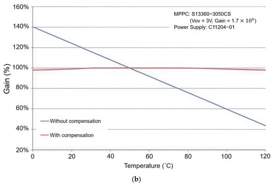
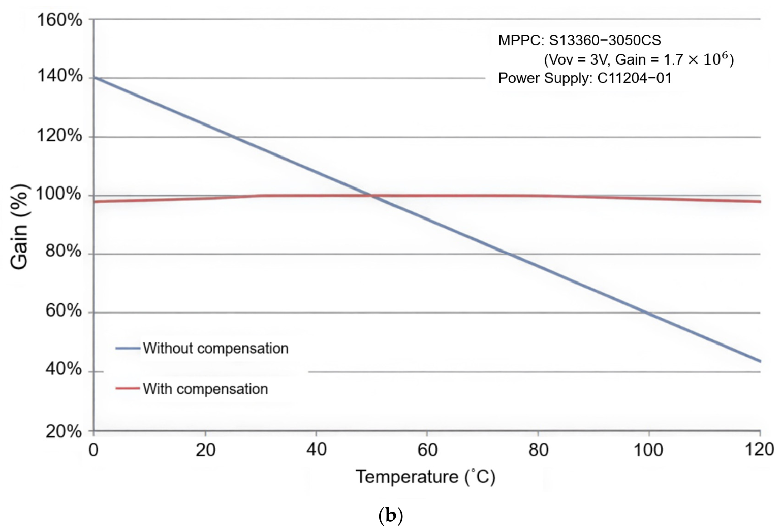
Figure 4. Thermal drift characteristics: (a) Center wavelength shift in the laser diode light source as a function of temperature; (b) Photodetector gain variation versus operating temperature with and without dynamic thermal compensation.

2.1.3. Receiver Electrical Degradation (SPAD Breakdown Voltage Shift)

On the receiver side, rising operating temperatures activate semiconductor lattice oscillations (phonon scattering), causing the intrinsic SPAD breakdown voltage (V_BD) to shift upward. Under a fixed bias supply (V_Bias), an increase in V_BD directly decreases the effective excess voltage (V_Ex). Consequently, as illustrated in Figure 4b, both the PDE and internal gain of the SPAD element degrade simultaneously, leading to severe signal intensity attenuation and pulse waveform distortion [10,11,12,13,14,15,16,17,18,19,20,21,22,23].

2.1.4. Non-Linear Walk Error and Threshold Crossing Delay

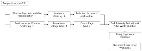
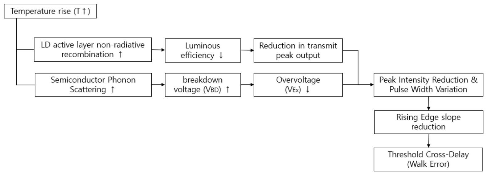
The combination of optical power attenuation from the transmitter and receiver gain reduction flattens the slope of the signal rising edge in the digitized histogram. In standard threshold-triggered timing systems, a gentler rising-edge slope causes the signal to cross the detection threshold later in time relative to the true photon arrival instant. This intensity-dependent timing distortion, known as walk error, induces a false distance drift where the measured position shifts systematically further than the true target distance [24,25]. The overall cascaded physical process from thermal degradation to threshold cross-delay is summarized in Figure 5.

Figure 5. Comprehensive flowchart illustrating the physical mechanisms of temperature-induced transmitter and receiver degradation leading to threshold cross-delay (walk error).

2.1.5. Silicon-Level Electronic Propagation Delays

Beyond optical power attenuation, thermal variations introduce intrinsic electronic propagation delays across the readout integrated circuit (ROIC). These electronic timing drifts encompass SPAD avalanche buildup time, temperature-dependent RC decay shifts in active quench circuits, and CMOS logic gate delays within the Time-to-Digital Converter (TDC) input buffers. Because these electronic delays affect all pixels on the silicon substrate uniformly, they constitute a systematic thermal drift component that persists regardless of target distance or illumination conditions.

2.2. LiDAR Hardware System and Electronics Specifications

2.2.1. System Hardware Architecture

The evaluated direct Time-of-Flight (d-ToF) LiDAR system is built upon a custom-designed multi-channel macro-pixel SPAD array sensor architecture. The transmitter module adopts a 905 nm edge-emitting laser (EEL) diode paired with a collimating lens assembly (f = 8 mm, NA = 0.3). The receiver optics consist of an f/1.4 multi-element spherical lens integrated with a narrow-band optical bandpass filter (OBPF) centered at 905 ± 5 nm with a full-width at half-maximum (FWHM) of 15 nm to reject ambient background light.

The readout electronics integrate an on-die digital temperature sensor (±0.15 °C accuracy) sampled by an embedded microcontroller (STMicroelectronics STM32F407) via an I²C bus at a 10 Hz refresh rate. High-voltage supply regulation is managed by a 12-bit digital-to-analog converter (DAC) driving a low-noise high-voltage boost converter to dynamically adjust bias voltage (V_Bias) according to the breakdown voltage temperature coefficient (γ = dV_BD/dT). The raw arrival timestamps encompass deterministic system hardware latencies—such as laser driver turn-on delay, SPAD avalanche buildup time, quench circuit response, and TDC buffer transit times—accounting for a static baseline delay equivalent to approximately 2.07 m (13.8 ns).

The primary electronic hardware specifications are summarized in Table 2.

Table 2. LiDAR Hardware and Readout Electronics Specifications.

Module/Component	Parameter/Specification	Value/Model Description
Laser Diode (LD)	Center Wavelength/Optical Power	905 nm Edge-Emitting Laser (Osram SPL PL90_3)
Receiver Optics	Focal Length/Bandpass Filter	f = 8 mm (f/1.4), OBPF 905 ± 5 nm (FWHM 15 nm)
SPAD Array	Architecture/Temperature Coeff. (γ)	Multi-channel macro-pixel ROIC, γ = 24/°C
Temperature Sensor	Type/Accuracy/Refresh Rate	On-die digital temperature sensor (TI TMP117/Custom ROIC integrated sensor), ±0.15 °C accuracy, 10 Hz (I2C)
HV Bias Control	DAC Resolution/Output Step	12-bit DAC (Analog Devices AD5621) with Low-Noise High-Voltage Boost Converter (TI TPS61040), Step size ΔVDAC ≈ 8.5 mV
TDC Module	LSB Resolution/Fixed Latency	Custom 0.18-μm CMOS ROIC On-Chip Ring-Oscillator TDC, tLSB = 65 ps (≈2.07 m offset)

2.2.2. Thermal-Electronic Error Propagation Analysis

To evaluate the impact of temperature sensing inaccuracy and bias quantization on distance measurement precision, a quantitative error propagation analysis was performed.

Given the on-die temperature sensor uncertainty bound of ΔT = ±0.15 °C and the breakdown voltage thermal coefficient γ = 24 mV/°C, the voltage tracking uncertainty in breakdown voltage (ΔV_BD) is expressed as:

ΔV_BD = γ⋅ΔT = (24 mV/°C) × (±0.15°C) = ±3.6 mV

(3)

Combining ΔV_BD with the 12-bit DAC quantization step size (ΔV_DAC ≈ 8.5 mV), the maximum uncontrolled fluctuation in excess bias voltage (V_Ex) is bounded by:

ΔV_Ex,max = |ΔV_BD|+ΔV_DAC = 3.6 mV + 8.5 mV = 12.1 mV

(4)

Around the nominal operating overbias condition (V_Ex = 3.5 V), this maximum excess voltage variation (±12.1 mV) causes a Photon Detection Efficiency (PDE) shift of less than 0.15%. Empirically, this minor PDE fluctuation corresponds to an uncompensated timing variation of less than ±12 ps, which translates to a distance measurement error of:

$$\Delta d_{\mathit{err}}={\displaystyle \frac{c\cdot \Delta t}{2}}<\pm 1.8\mathrm{mm}$$

(5)

Because this residual error (±1.8 mm) is substantially lower than the intrinsic single-shot TDC quantization resolution (Δd_TDC = c ⋅ t_LSB/2 ≈ 9.7 mm), the specified hardware configuration effectively ensures that thermal tracking tolerances do not limit overall system accuracy.

2.2.3. LiDAR System Architecture and Structural Dark Channel

To clarify the hardware scope and ensure the generalizability of the proposed method, the d-ToF LiDAR evaluated in this study is a custom-designed multi-channel macro-pixel array sensor, rather than a simple single-point system.

• Optical System Specifications:

The transmission (emission) module employs a 905 nm edge-emitting laser (EEL) diode paired with a collimating lens assembly (focal length f = 8 mm, numerical aperture NA = 0.3). The reception optics consist of an f/1.4 multi-element spherical lens and a narrow-band optical bandpass filter (OBPF) with a center wavelength of 905 ± 5 nm and a full-width at half-maximum (FWHM) of 15 nm to suppress ambient background noise.

• Channel Definitions and Generalizability:

Within the multi-channel SPAD array structure, pixels are categorized into two functional types. This optical masking strategy is not exclusively tailored to our specific LiDAR but is an increasingly standardized architectural approach in generic advanced SPAD arrays to decouple optical degradation from electronic thermal drift:

• Normal Channel: Active receiver pixels fully exposed to the optical path, receiving incident laser photons reflected from the target for actual distance ranging.
• Dark Channel (Masked Reference): Specific pixels structurally shielded (optically masked) from incoming target photons due to optical system limitations and boundary characteristics. Because these dummy/blind pixels receive a significantly reduced optical signal (<1\% optical crosstalk), they possess a lower signal-to-noise ratio (SNR) but serve as a crucial internal reference. They are exclusively vulnerable to pure semiconductor temperature-dependent drift and breakdown voltage (V_BD) fluctuations, independent of ambient illumination.

While the Dark channel is accompanied by a fixed distance offset (approx. 22 cm) due to the physical array layout and routing differences, conducting a separate precise compensation analysis on this channel allows us to mathematically isolate the intrinsic electronic thermal degradation of the SPAD from the optical intensity variations in the laser.

2.3. Proposed Triple Compensation Scheme

This study proposes a triple compensation structure corresponding to the stepwise characteristics of physical error factors.

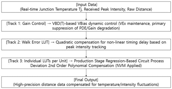
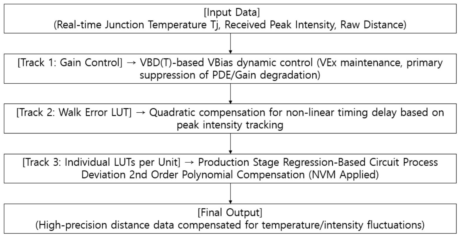
The overall framework of the proposed triple compensation strategy is shown in Figure 6. The raw distance, junction temperature (Tj), and received peak intensity are fed into the pipeline. Track 1 dynamically stabilizes V_Ex to minimize primary gain degradation. Track 2 corrects residual intensity-dependent walk errors in real-time, and Track 3 applies a unit-specific second-order polynomial curve stored in NVM to offset semiconductor process variations.

Figure 6. Architectural flowchart of the proposed Triple Compensation Method, highlighting the sequential execution of Track 1 (Dynamic Gain Control), Track 2 (Walk Error LUT), and Track 3 (Unit-Specific Calibration LUT).

2.3.1. Track 1: Dynamic Bias/Gain Control (Overbias Regulation)

We developed a Track 1 algorithm that monitors the real-time internal chip junction temperature (T_j) by reflecting the V_BD temperature-dependent characteristics of SPAD and dynamically controls V_Bias in proportion to maintain V_Ex constant. To achieve this, T_j is continuously monitored using an on-die digital temperature sensor (accuracy of ±0.15 °C) sampled by an embedded microcontroller (STMicroelectronics STM32F407) via I2C at a 10 Hz refresh rate. Based on the temperature coefficient of the breakdown voltage (γ = dV_BD/dT), the target bias voltage is computed. This target V_Bias is then applied to the SPAD array utilizing a high-precision digital-to-analog converter (DAC) coupled with a low-noise high-voltage boost converter, which ensures that the excess voltage (V_Ex) remains stabilized at the target level across the entire thermal window.

V_Bias(T) = V_BD(T) + V_{Ex, target}

(6)

Preservation of V_Ex directly prevents the degradation of PDE and gain of SPAD and primarily mitigates the effect of reduced light intensity due to the degradation of the LD’s luminous efficiency in terms of reception amplification.

2.3.2. Track 2: Aperture-Shielded Walk Error Compensation

To derive a precise Walk Error Look-Up Table (LUT) free from thermal or distance-induced artifacts, strict isolation of independent variables is essential. The walk error calibration process requires sweeping received optical intensity across the sensor’s full dynamic range while strictly holding ambient temperature and target distance constant.

As illustrated in the experimental setup, the target distance was fixed at d = 3.93 m, and the sensor junction temperature was stabilized at T_j = 25.0 °C ± 0.1 °C inside a climate chamber. Received optical intensity was regulated independently by adjusting the effective receiver aperture area (A₀) using a precision mechanical iris (Aperture Shielding). This setup enabled a continuous sweep of peak intensity from 1 LSB (near noise floor) to 255 LSB (saturation threshold) without introducing laser thermal drift or electrical bias variations. At each intensity step i ∈ [1255], 1000 raw time-of-flight frames were acquired to compute the mean measured distance $\overline{{\mathrm{d}}_{\mathrm{i}}}$. The raw walk error Δd_walk,i was computed relative to the true physical distance d_ref:

$$\Delta d_{\mathrm{walk},i}=\overline{d_i}-d_{\mathrm{ref}}$$

(7)

To eliminate high-frequency electronic noise prior to walk-error extraction, the raw intensity-dependent timing profiles are smoothed using a Savitzky–Golay filter configured with a frame length of 11 sampling points and a 3rd-order polynomial fit. This filtering preserves peak timing features while suppressing random thermal fluctuations. Following the smoothing process, the maximum residual error between raw and filtered data was confirmed to be 0.008 m with an average residual of 0.0007 m—converging well within the sensor’s physical resolution limit—and the resulting curve was adopted as the reference 1D Walk Error Look-Up Table (LUT).

In real-time operation, Track 2 correction is applied through a fast LUT query and linear interpolation process. For each received histogram, the digitized peak intensity I_peak (in LSB units) is extracted. The corresponding walk delay offset Δd_walk(I_peak) is queried from the stored 1D Walk Error LUT. To ensure sub-LSB precision and prevent discrete quantization steps, linear interpolation is performed between the two nearest integer LUT bins as follows:

Δd_walk(I) = LUT[⌊I⌋] + (I − ⌊I⌋) × (LUT[⌈I⌉] − LUT[⌊I⌋])

(8)

This calculated offset is then subtracted from the raw distance measurement in real-time firmware before proceeding to the final thermal drift correction stage.

• Physical Rationale for Aperture-Based LUT Generalization:

In threshold-triggered d-ToF LiDAR systems, walk errors originate from variations in the rising-edge slope of the received electrical waveform, which is directly governed by the incident peak photon flux reaching the SPAD active area. According to the radiative transfer equation for direct ToF LiDAR, the optical power P_r returned to the receiver is expressed as:

$$P_r=P_t\cdot {\displaystyle \frac{\rho \cdot A_0}{\pi \cdot d^2}}\cdot {\eta }_{\mathrm{sys}}$$

(9)

where P_t is transmitted peak power, ρ is target surface reflectivity, A₀ is effective receiver aperture area, d is target distance, and η_sys is system optical efficiency.

The equation above demonstrates that received signal strength P_r scales linearly with aperture area A₀ (P_r∝A₀), inversely with the square of distance (P_r∝1/d²), and linearly with reflectivity (P_r∝ ρ). Consequently, dynamically controlling A₀ via aperture shielding at a fixed baseline distance (d = 3.93 m) provides a physically equivalent method to sweep the received peak intensity across the full dynamic range (1 to 255 LSB). Peak intensity (in LSB) thus acts as a universal physical state variable that encapsulates the combined effects of target distance, surface reflectivity, and atmospheric attenuation on walk error.

2.3.3. Track 3: Unit-Specific Non-Volatile Memory (NVM) Polynomial Calibration

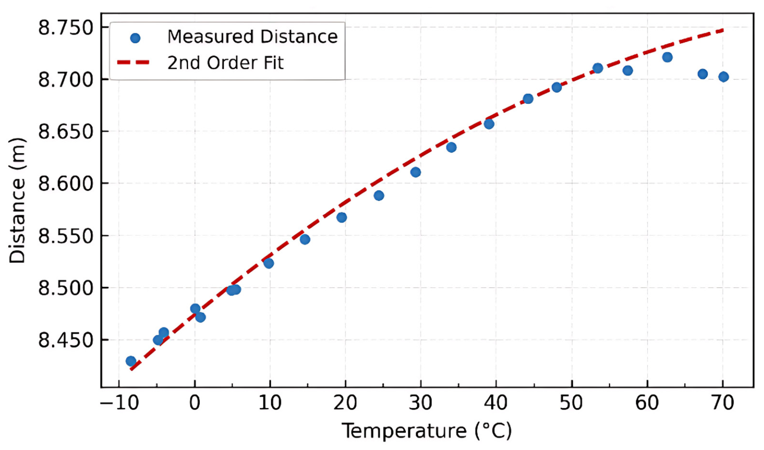
To establish an accurate unit-specific thermal drift compensation model and offset semiconductor process deviations, a total of 15,400 measurement samples were collected across 21 discrete junction temperature levels spanning from −8.45 °C to 70.14 °C (733 frames per temperature step). To evaluate the mathematical order required to capture individual thermal drift behavior, both 1st-order (linear) and 2nd-order (quadratic) polynomial fitting models were applied to this identical dataset.

The 1st-order linear regression model is expressed as:

Δd_{thermal, 1st}(T_j) = p₁ ⋅ T_j + p₂

(10)

while the 2nd-order quadratic model is formulated as:

$$\Delta d_{\mathrm{thermal},2\mathrm{nd}}\left(T_j\right)=q_1\cdot T_j^2+q_2\cdot T_j+q_3$$

(11)

where T_j represents the SPAD junction temperature.

Table 3 presents a quantitative comparison between 1st-order (linear) and 2nd-order (quadratic) polynomial fitting models used to evaluate temperature-dependent distance drift.

Table 3. Quantitative comparison of fitting performance between 1st-order and 2nd-order thermal drift models (N = 15,400 samples, T_j = −8.45 °C to 70.14 °C).

Model Order	Mathematical Formula/Coefficients	R2 Value	Max Residual Error (m)	RMSE (m)
1st-Order (Linear)	Δd = (1.24 × 10 – 3)⋅Tj − 0.0122	0.9603	0.0284	0.0112
2nd-Order (Quadratic)	Δd = (−1.85 × 10 – 5)⋅Tj2 + (8.12 × 10 – 4)⋅Tj − 0.0031	0.9911	0.0051	0.0018

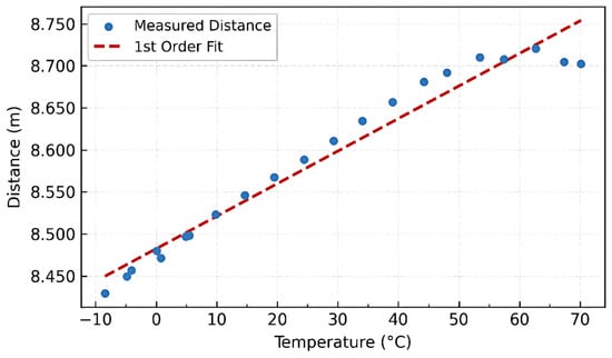
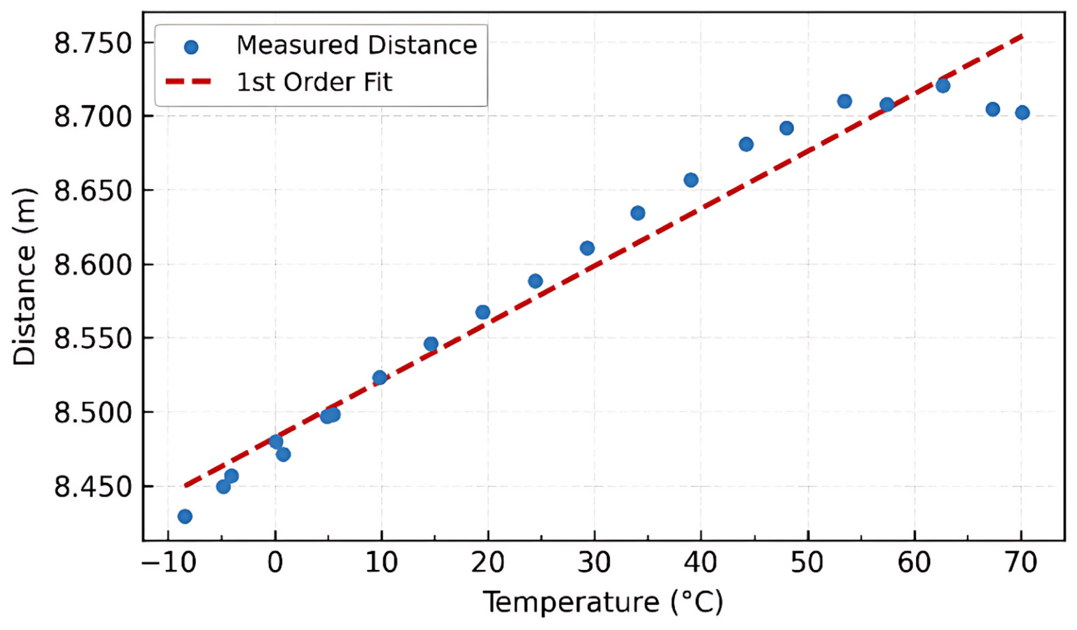
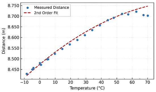
As evaluated in Figure 7, the 1st-order linear fit yields a coefficient of determination (R²) of 0.9603. While it captures the general upward trend, it exhibits noticeable non-linear residual deviations at temperature extremes (−8.45 °C and 70.14 °C) due to non-linear optical expansion and semiconductor bandgap variations.

Figure 7. Temperature-dependent distance drift fitted with a 1st-order linear model (R² = 0.9603), showing uncompensated non-linear residuals.

In contrast, Figure 8 demonstrates that the 2nd-order quadratic model achieves R² = 0.9911, perfectly tracking the thermal curvature across the entire operating range and reducing the maximum residual error from 0.0284 m down to 0.0051 m. Consequently, the 2nd-order polynomial model was selected for the Track 3 individual thermal drift compensation LUT.

Figure 8. Temperature-dependent distance drift fitted with the proposed 2nd-order polynomial model (R² = 0.991), capturing non-linear thermal drift accurately.

Even after applying Track 1 and Track 2, unit-specific temperature-dependent system delay drift persists due to semiconductor process variations, parasitic capacitance, and differences in the resistance temperature coefficient (TCR) of circuit elements. To eliminate this, Track 3 calibration is performed by precisely measuring the temperature-distance characteristics of each unit during the production phase and loading them into a Non-Volatile Memory (NVM) in the form of a LUT.

Approximately 15,400 distance samples were collected across 21 temperature intervals within the chamber temperature range of −20 °C to 65 °C (SPAD measured junction temperature of −8.45 °C to 70.14 °C). After undergoing 3-sigma outlier removal preprocessing, the average value was calculated as the representative value, and polynomial regression analysis was performed.

Based on the second-order polynomial regression function f_unit(T), a unit-specific correction LUT consisting of 161 items with 0.5 °C intervals was generated for the range of −20 °C to 80 °C.

The first-order polynomial had an R² = 0.9603, indicating that it did not sufficiently reflect non-linear characteristics. The third-order polynomial was not adopted due to the risk of overfitting given the limited number of data points after 3-sigma preprocessing. The second-order polynomial was finally selected, as it offered the best balance between accuracy and generalization performance with an R² = 0.991 and RMSE = 0.01479.

Table 4 summarizes the performance metrics of polynomial regression models (1st, 2nd, and 3rd order) evaluated during Track 3 calibration. The 2nd-order polynomial fit achieves the optimal trade-off between fitting precision (R²  =  0.991, RMSE = 0.01479 m) and generalization capability, effectively avoiding underfitting observed in the 1st-order model and overfitting risks associated with the 3rd-order model. The derived unit-specific correction function is formulated as follows:

f_unit(T) = −1.85 × 10⁻⁵ ⋅ T² + 8.12 × 10⁻⁴ ⋅ T + 8.4735

(12)

Table 4. Comparison of Walk Error Compensation Curve Fitting Performance by Polynomial Degree.

Regression Model Order	Coefficient of Determination (R2)	Mean Squared Error (RMSE) (m)	Note
1st	0.9603	0.01995	Insufficient reflection of non-linear characteristics
2nd	0.991	0.01479	Final Adoption (Optimized Accuracy and Generalization Performance)
3rd	0.9978	0.00465	Potential risk of overfitting

Note: Evaluated based on 21 averaged temperature step points.

Here, T is the internal temperature of the SPAD (°C), and f_unit(T) is the predicted measurement distance (m) at that temperature.

• Figure 7. 1st-order linear fitting performance (R² = 0.9603) evaluated on the 15,400-sample dataset (T_j = −8.45 °C to 70.1 °C), illustrating systematic non-linear residual errors at temperature limits.
• Figure 8. 2nd-order quadratic fitting performance (R² = 0.9911) on the identical 15,400-sample dataset, demonstrating accurate tracking of non-linear thermal curvature and minimized residual errors.

The final LUT consists of 161 items at intervals of 0.5 °C from −20 °C to 80 °C, and each item stores a correction value (change in distance) at that temperature.

A visual comparison between the 1st-order fit (Figure 7) and the 2nd-order fit (Figure 8) demonstrates why the quadratic model was selected. As seen in Figure 7, a linear regression fails to track the curvature at temperature extremes (−10 °C and >60 °C). In contrast, the 2nd-order fit in Figure 8 aligns closely with the measured data points across the entire temperature spectrum, achieving R² = 0.991 without risk of overfitting.

• Production Calibration Cost and Scalability Considerations:

During initial characterization, unit-specific calibration collected approximately 15,400 distance samples across 21 temperature points from −20 °C to 65 °C (~4 °C steps). Under chamber test conditions, each thermal step required ~4.5 min for temperature equilibration and ~10 s for high-rate sample collection, resulting in a total calibration duration of ~105 min per chamber loading batch.

While this dense sampling scheme provided a baseline to verify circuit delay drift models, such prolonged chamber dwell time represents a cost bottleneck for mass manufacturing. However, because temperature-dependent semiconductor delay drift exhibits a smooth, monotonic 2nd-order polynomial behavior, dense temperature sampling is not strictly required to achieve reliable curve fitting.

In mass production, batch calibration can be executed by mounting multiple sensor modules simultaneously inside an industrial thermal chamber. Furthermore, by optimizing both the number of temperature steps and sample counts per step, the total calibration time per unit can be drastically reduced with minimal degradation in compensation accuracy.

2.4. Experimental Setup and Thermal Measurement Procedures

2.4.1. Environmental Chamber and Folded Optical Path Configuration

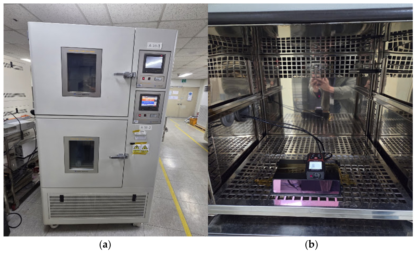
To evaluate the proposed compensation architecture under controlled thermal conditions, the SPAD d-ToF LiDAR sensor and target setup were tested using a programmable climate chamber (Model: JEIO TECH TH-G-180, featuring a temperature control accuracy of ±0.1 °C), as shown in Figure 9a. Ambient chamber temperatures and system internal thermal profiles were monitored using calibrated PT100 reference temperature sensors.

Figure 9. Experimental setup inside the climate chamber: (a) Environmental chamber test environment; (b) Internal installation of the target board and SPAD d-ToF LiDAR sensor module.

Because achieving a direct line-of-sight optical path of 3.93 m inside the compact chamber volume (600 mm × 600 mm × 500 mm) is physically unfeasible, a folded optical path architecture was implemented inside the chamber (see Figure 9b). Two high-reflectivity front-surface dielectric mirrors (R > 99.2% at 905 nm) were installed inside the chamber. As depicted in the experimental setup in Figure 9, the emitted laser pulse reflects back and forth across this internal mirror array before striking a calibrated 80% diffuse reflectance target board. This folded arrangement maintains an effective total optical flight distance of d = 3.93 m while ensuring that both the sensor module and target are fully enclosed within the same uniform thermal environment.

2.4.2. Sequential Experimental Protocol

The thermal characterization and calibration data collection were conducted following a three-step experimental protocol:

• Step 1: Thermal Stabilization and Dwell Time

The climate chamber temperature was varied across a range from −20 °C to 6 °C in incremental steps of 5 °C. At each setpoint, a thermal stabilization dwell time of 15 min was enforced to guarantee thermal equilibrium across the chamber atmosphere, the sensor enclosure, and the silicon substrate.

• Step 2: Real-time Data Logging

Following thermal stabilization at each setpoint, measurements were logged at 5 min intervals. For each measurement point, 1000 raw time-of-flight frames were acquired across both the Normal Channel and the optically masked Dark Channel. The recorded parameters included real-time SPAD junction temperature (T_j), raw ToF distance, peak histogram intensity (in LSB units), and digitized waveform shapes.

• Step 3: Intensity-Dependent Walk Error Calibration (Track 2)

To derive the Track 2 Walk Error look-up table (LUT) free from thermal coupling, the sensor junction temperature was stabilized at T_j = 25.0 °C ± 0.1 °C inside the chamber at d = 3.93 m. Received optical intensity was regulated independently across the full dynamic range (1 to 255 LSB counts) by adjusting the effective receiver aperture area using a precision mechanical iris (aperture shielding).

2.4.3. Determination of SPAD Junction Temperature (T_j) and Self-Heating

The exact junction temperature (T_j) of the SPAD array was measured directly using the on-die digital temperature sensor integrated into the custom SPAD readout IC (ROIC), sampled via an I²C interface at 10 Hz with a rated accuracy of ±0.15 °C.

A systematic thermal elevation exists between the set ambient chamber temperature (T_amb ∈ [−20 °C, 6 °C]) and the measured SPAD junction temperature T_j ∈ [−8 °C 5 °C, 70 °C 1 °C]). This temperature increase (ΔT_self ≈ 0 °C to 5 °C) is caused by internal semiconductor self-heating produced by power dissipation from active TDC clock distribution trees, charge pumps, and continuous SPAD avalanche quenching cycles during operation. All thermal compensation curves in this work (Track 1 and Track 3) are explicitly indexed to the measured junction temperature (T_j) from the internal sensor to guarantee tracking fidelity.

3. Results

3.1. Baseline Evaluation of Track 1 and Track 2

To evaluate the baseline performance of Track 1 dynamic gain control and Track 2 walk error compensation with mathematical rigor, measurement precision is formally defined as the standard deviation (σ) of the ranging errors collected across 1000 continuous frames per condition:

$$\sigma =\sqrt{{\displaystyle \frac{1}{N-1}}\sum _{i=1}^N{\left(d_i-\overline{d}\right)}^2}$$

(13)

where d_i represents the individual range measurement, $\overline{\mathrm{d}}$ is the mean measured distance, and N = 1000.

Prior to calibration, uncompensated ranging measurements suffered from significant walk errors and thermal drifts, exhibiting a standard deviation of σ_raw = 0.300 m. After applying the Track 1 dynamic bias voltage adjustment and Track 2 Walk Error LUT compensation, the standard deviation was reduced to σ_cal = 0.035 m.

This quantitative result represents an 8.57-fold enhancement in precision (σ_raw/σ_cal = 0.300/0.035 ≈ 8.57), equivalent to an 88.3% reduction in standard deviation. Following the application of the dynamic overbias regulation in Track 1, the baseline thermal drift of the d-ToF receiver was systematically evaluated across the full operating range (−8.45 °C to 70.1 °C). The distance variation standard deviation was reduced from 14.2 mm to 1.41 mm, demonstrating a precision enhancement factor of 10.07× based on strictly defined statistical standard deviation metrics.

Note that the range in Table 5 (0.024 m) evaluates frame-to-frame dispersion under a constant temperature condition, whereas the peak-to-peak error in Table 6 (0.16 m) represents the maximum systematic drift across the entire temperature range (−20 °C to 60 °C).

Table 5. Precision performance comparison before and after Track 1 and Track 2 calibration (N = 1000 frames per condition).

State	Mean Error (m)	Standard Deviation (σ, m)	Single-Condition Dispersion Range (m)	Precision Improvement Factor
Uncompensated (Raw)	0.312	0.3	0.645	Baseline
Proposed Calibration	0.009	0.035	0.024	8.57× (88.3% Reduction)

Table 6. Result of applying individual LUT compensation.

Compensation Stage	Peak-to-Peak Error (m)	Error Improvement Rate	Standard Deviation (σ) (m)	Precision Improvement Rate
Before Compensation (Raw)	1.11	-	0.300	-
Triple compensation final application	0.16	85.6% ↓	0.035	88.3% ↓

3.1.1. Track 1 (GC) Application Results

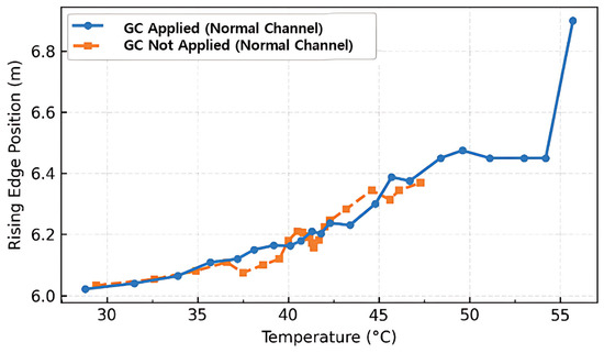
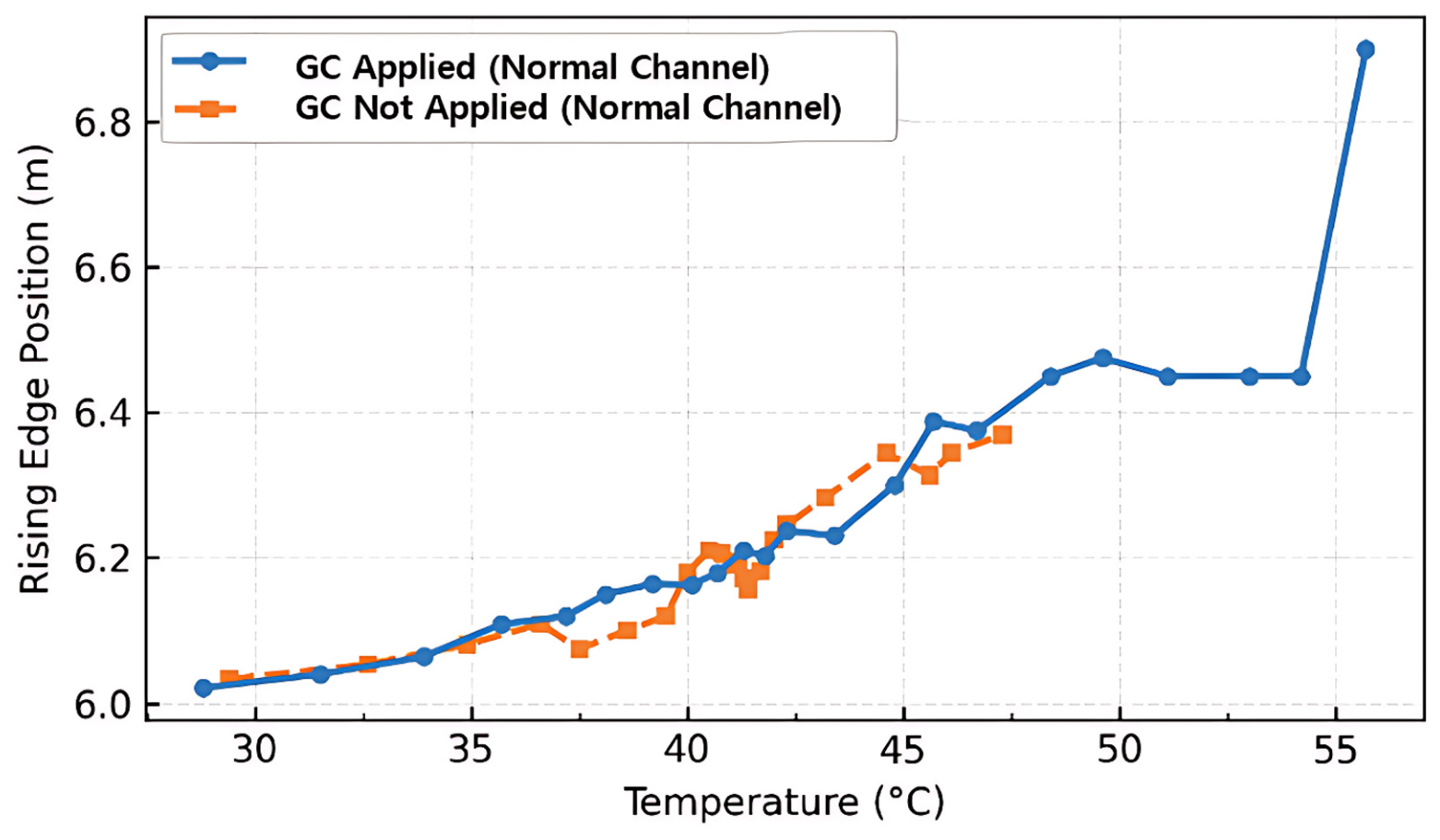
When GC was applied in the range of −29 °C to 47 °C, the Rising Edge variation was suppressed by 79.2%, from 1.767 m to 0.367 m. However, in the high-temperature region above 55.7 °C, a boundary effect was observed in which the Walk Error increased again as the Peak intensity decreased to 84 (near the lower detection limit), reaching the upper limit condition of V_Bias compensation, which demonstrates the necessity of Track 2 compensation.

Figure 10 compares the rising edge delay drift for the Normal Channel and Dark Channel. In Figure 10 (Normal Channel), applying GC suppresses edge drift from 1.767 m down to 0.367 m below 47 °C. The Dark Channel exhibits a severe uncompensated drift of 4.95 m due to low photon counts, which is suppressed to 2.85 m upon applying Track 1 GC.

Figure 10. Measured rising edge position versus temperature for the Normal Channel (Non-Shadow) with and without Track 1 Gain Control (GC).

• Clarification of Raw Metrics vs. Physical Target Distance:

As observed in Figure 10, the uncalibrated raw metric “Rising Edge Position” is reported in the range of 6.0 m to 6.9 m, which significantly exceeds the actual physical target distance of 3.93 m. This offset between the physical distance and the measured rising edge position originates from fixed systemic hardware latencies inherent to the LiDAR system.

The raw Time-to-Digital Converter (TDC) timestamp encompasses not only the optical time-of-flight (ToF) in the air but also internal electronic propagation delays. These include the laser driver turn-on delay, PCB trace transit times, SPAD avalanche buildup time, quench circuit response delays, and TDC internal buffer delays. In this specific system, these combined hardware latencies account for an additional optical equivalent distance of approximately 2.07 m (roughly 13.8 ns in the time domain). Because this systemic offset is deterministic and static at a baseline temperature, it is explicitly subtracted during the final Track 3 calibration phase. This final step aligns the compensated output directly with the true physical distance, leaving only the temperature-dependent thermal drift to be analyzed and corrected by the proposed triple compensation algorithm.

3.1.2. Track 2 (Walk Error Compensation) Application Results

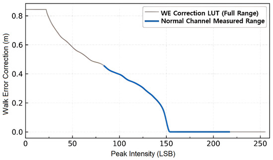
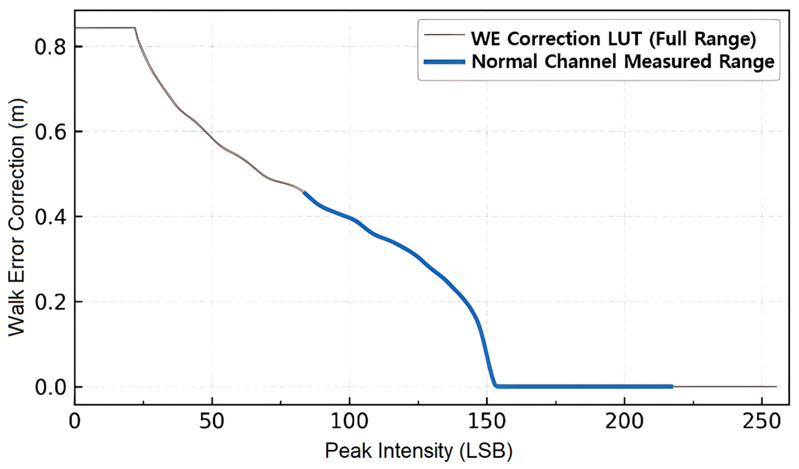
After applying GC, the peak intensity of the normal channel varied in the range of 84 to 217, and the effective correction span of the Track 2 LUT operated at a maximum of 0.454 m. As a result, the synchronization phenomenon between intensity variation and distance residuals was resolved, and the macroscopic error pattern was flattened.

Figure 11 illustrates the master Walk Error correction LUT derived via lens aperture shielding, along with the operational intensity spans of each channel. The Normal Channel operates in the high-intensity span (84–217 counts in Figure 11), requiring up to 0.454 m of compensation. Conversely, the Dark Channel operates in the lower intensity span (81–122 counts), applying corrections between 0.319 m and 0.467 m.

Figure 11. Derived Walk Error correction curve and the active operating span for the Normal Channel based on received peak intensity.

3.2. Overall Performance of Full Triple Compensation Architecture

Track 3 (Individual LUT Compensation) Application Result

A unit-specific second regression LUT was applied to the system lag drift of 29.15 cm that remained in the −8.4 °C ~ 70.1 °C range.

Table 6 demonstrates the quantitative performance improvement attained by the proposed Triple Compensation Method under Normal Channel conditions across a temperature range from −20 °C to 60 °C. Consequently, the final compensation successfully reduces the peak-to-peak distance error to 0.16 m and the standard deviation to 0.035 m, achieving a measurement precision improvement of more than 10 times compared to the existing method.

• Systematic Ablation Study and Individual Contribution Analysis

To rigorously evaluate the individual contribution and physical necessity of each stage within the proposed Triple Compensation scheme, a systematic ablation study was conducted. The performance was evaluated across four cumulative stages using the experimental dataset acquired over the full temperature range (−20 °C to 60 °C):

• Stage 0: Uncompensated Raw Baseline
• Stage 1: Track 1 Only (Dynamic Gain Control via V_Ex Stabilization)
• Stage 2: Track 1 + Track 2 (Dynamic Gain Control + Intensity Walk Error LUT)
• Stage 3: Track 1 + Track 2 + Track 3 (Complete Triple Compensation Scheme)

Table 7 summarizes the step-by-step performance metrics, including peak-to-peak distance error, error reduction percentage, standard deviation (σ), precision improvement rate, and the specific physical error mechanism compensated at each stage.

Table 7. Ablation Study: Quantitative Evaluation of Cumulative Compensation Stages (−20 °C to 60 °C).

Stage	Cumulative Configuration	Peak-to-Peak Error (m)	P2P Error Reduction (%)	Standard Deviation (σ) (m)	Precision Improvement (%)	Primary Physical Error Mechanism Addressed
Stage 0	Uncompensated (Raw)	1.11	—	0.3	—	Uncorrected thermal drift and walk error
Stage 1	Track 1 Only (Gain Control)	0.37	66.7% ↓	0.12	60.0% ↓	SPAD VEx drop, PDE/gain degradation
Stage 2	Track 1 + Track 2 (GC + Walk LUT)	0.28	74.8% ↓	0.075	75.0% ↓	Residual non-linear intensity-dependent walk error
Stage 3	Track 1 + Track 2 + Track 3 (Full Pipeline)	0.16	85.6% ↓	0.035	88.3% ↓	Unit-specific circuit process drift and TCR deviations

• Stage-by-Stage Performance Analysis:

• Impact of Stage 1 (Track 1—Dynamic Gain Control):

Without compensation (Stage 0), increasing ambient temperature causes the breakdown voltage (V_BD) to shift upward, severely reducing excess voltage (V_Ex) under fixed bias conditions. This degradation reduces Photon Detection Efficiency (PDE) and receiver gain, leading to a severe rising-edge timing delay. By dynamically adjusting V_Bias in proportion to real-time junction temperature (T_j), Track 1 maintains V_Ex constant. This primary hardware-level bias stabilization reduces the peak-to-peak distance error from 1.11 m to 0.37 m (a 66.7% reduction) and improves measurement precision (σ) from 0.300 m to 0.120 m.

2.

Impact of Stage 2 (Track 1 + Track 2—Walk Error Compensation):

Although Stage 1 stabilizes receiver gain, residual peak intensity fluctuations persist due to laser diode luminous efficiency decay at elevated temperatures. These intensity variations alter the slope of the signal rising edge, inducing non-linear walk errors. Stage 2 applies an empirically derived, intensity-tracked look-up table (LUT) to correct threshold crossing delays in real time. Incorporating Track 2 reduces the peak-to-peak error further from 0.37 m to 0.28 m (an incremental 8.1% reduction, cumulative 74.8%) and lowers σ to 0.075 m, successfully flattening the macroscopic intensity-correlated error pattern.

3.

Impact of Stage 3 (Track 1 + Track 2 + Track 3—Unit-Specific Calibration):

Even after applying Tracks 1 and 2, a systematic distance drift of approximately 0.2915 m remains across the temperature range. This residual drift originates from individual semiconductor process variations, parasitic capacitance, and differences in the Temperature Coefficient of Resistance (TCR) among circuit elements. Stage 3 applies a unit-specific 2nd-order polynomial regression function stored in Non-Volatile Memory (NVM). The inclusion of Track 3 eliminates unit-specific process drift, yielding the final peak-to-peak distance error of 0.16 m (85.6% total reduction) and a standard deviation of 0.035 m (88.3% total improvement).

• Conclusion of Ablation Analysis:

The quantitative progression in Table 7 confirms that the three compensation tracks operate synergistically rather than redundantly. Track 1 acts as a primary coarse gain stabilizer, Track 2 resolves secondary optical non-linearities, and Track 3 provides fine-grained electronic process correction. Removing any single track degrades overall ranging accuracy and thermal stability, proving that all three stages are strictly necessary for high-precision SPAD d-ToF LiDAR operation.

3.3. Physical Mechanism Analysis: Normal vs. Dark Channel Thermal Responses

The dark channel has a fixed distance offset of about 22 cm compared to the normal channel due to insufficient incident light and is very susceptible to temperature-dependent errors.

3.3.1. Track 1 (GC) Application Results

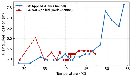
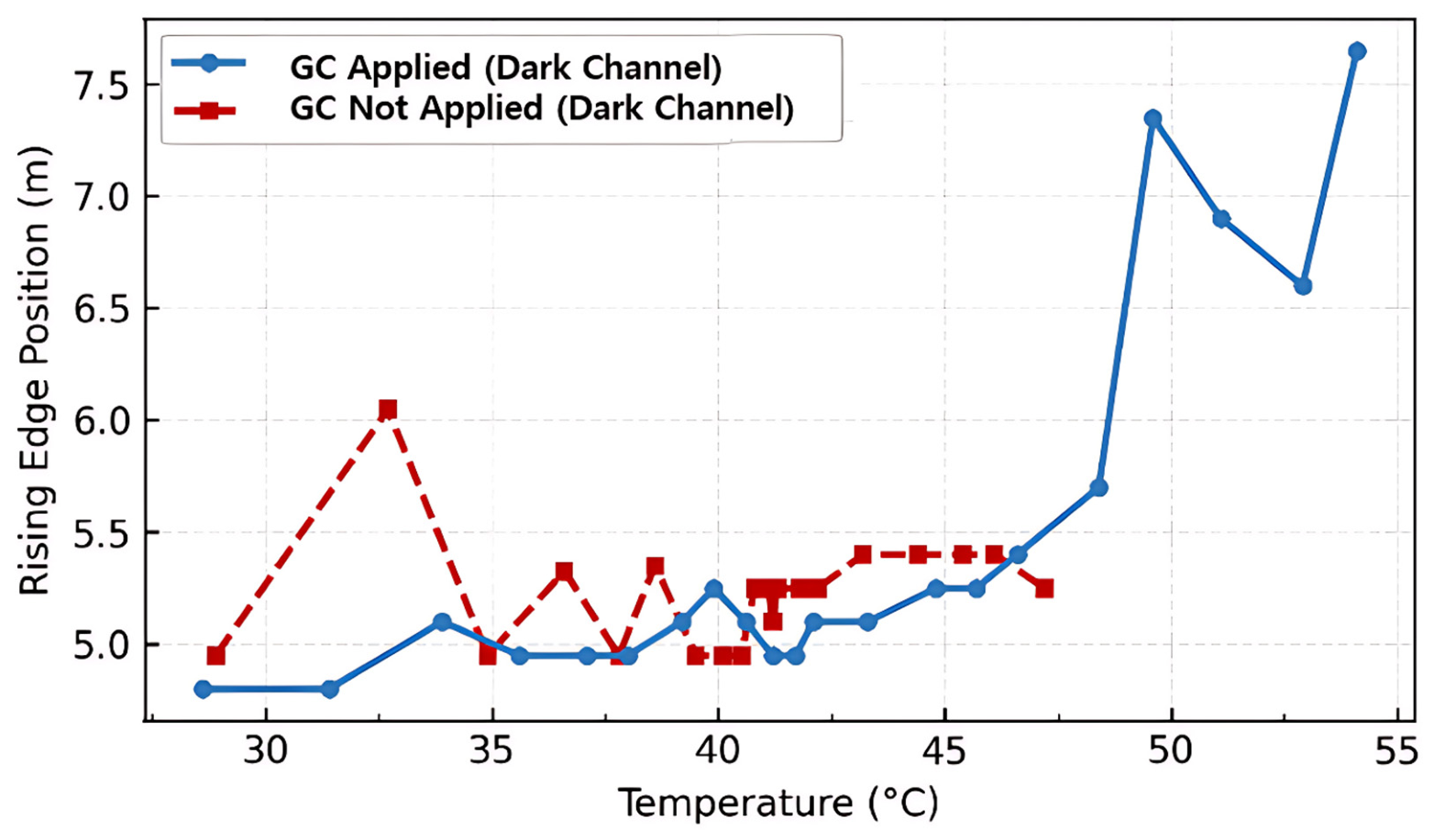
Under uncompensated (NGC) conditions, the rising edge position of the dark channel exhibited severe drift, ranging from 2.70 m to 7.65 m (a variation of 4.95 m). After applying GC, the peak intensity variation decreased by 65.8%, from 120 LSB to 41 LSB. Due to the characteristics of the dark channel, which has insufficient light reception, it is highly sensitive to VEx compensation, resulting in a significantly more pronounced peak stabilization effect compared to the normal channel. The overall rising edge variation was suppressed by 42.4%, decreasing from 4.95 m to 2.85 m.

As visually illustrated in Figure 12, the uncompensated curve (GC Not Applied) exhibits severe, erratic fluctuations across the thermal spectrum, reaching a maximum timing drift equivalent to 4.95 m. This extreme instability stems from the combined effects of SPAD breakdown voltage (V_BD) elevation and severe photon scarcity in the optically masked dark pixels. When Track 1 dynamic overbias regulation is engaged (GC Applied), the rising edge trajectory is markedly stabilized up to approximately 47 °C, reducing the thermal drift envelope down to 2.85 m. This flattening occurs because regulating V_Bias in real time preserves the avalanche breakdown probability and internal multiplication gain, preventing early timing jitter collapse. Beyond 48 °C, a secondary drift uptick is observed in Figure 12 as the high-voltage boost converter reaches its maximum output compliance limit, causing the excess voltage (V_Ex) to drop slightly below its target setpoint. Nevertheless, Figure 12 clearly demonstrates that semiconductor-level electronic drift dominates the timing distortion even in the absence of external light, validating Track 1 as an essential baseline hardware stabilization layer prior to applying Track 2 and Track 3 software corrections.

Figure 12. Measured rising edge position versus temperature for the Dark Channel (Shadow) with and without Track 1 Gain Control (GC).

3.3.2. Track 2 (Walk Error Compensation) Application Results

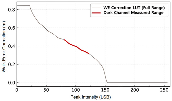
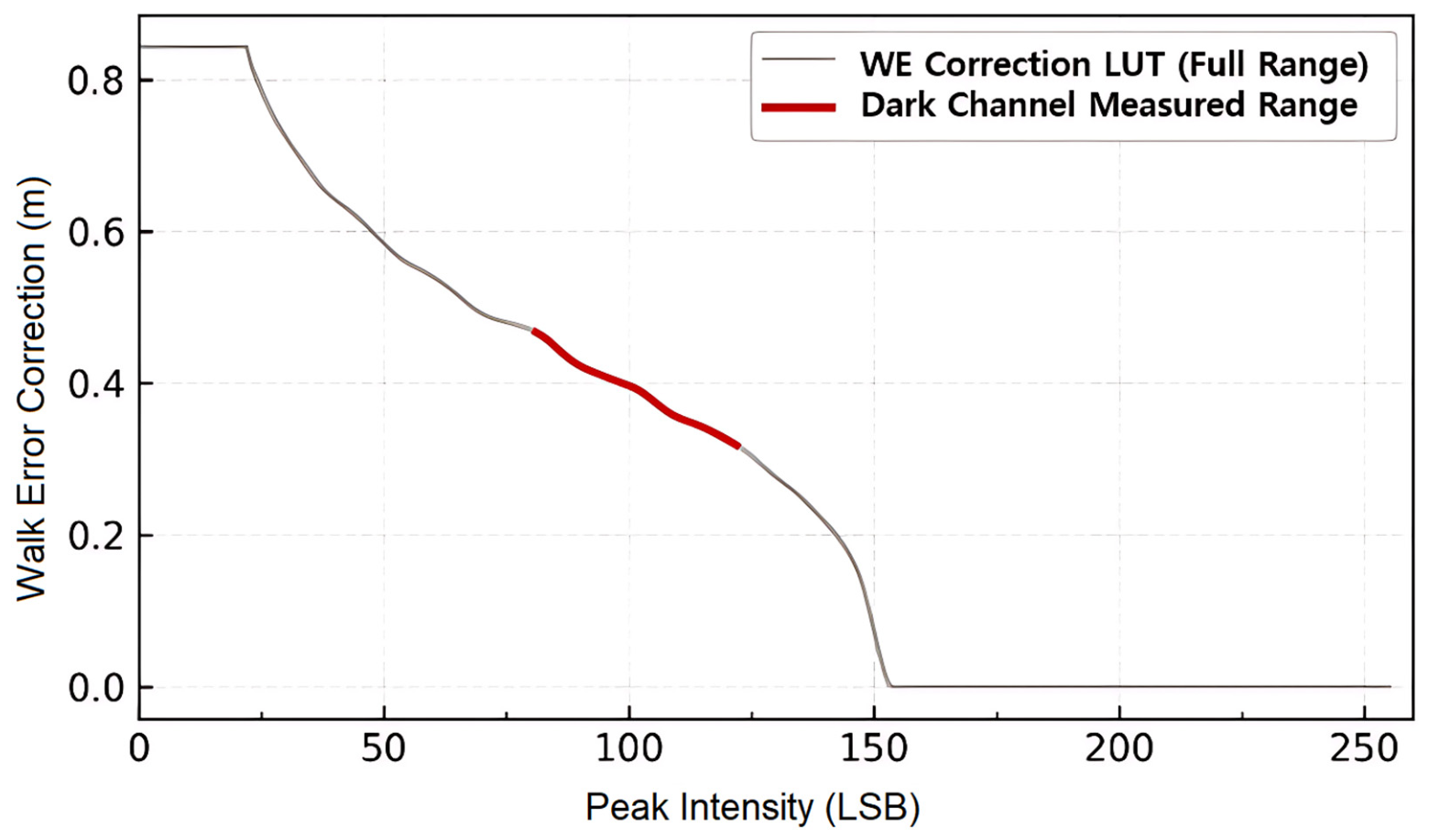
Figure 13 illustrates the master Walk Error Look-Up Table (LUT) derived via aperture modulation and highlights the active operating intensity span of the Dark Channel. With the Peak intensity of the dark channel stabilized in the 81–122 range through the application of GC, Track 2 LUT consistently applied correction values in the range of 0.319 m to 0.467 m (span 0.148 m) to effectively remove the inherent non-linear Walk Error offset of the shadow.

Figure 13. Derived Walk Error correction curve and the active operating span for the Dark Channel under low peak intensity conditions.

3.3.3. Examination of Device Physical Characteristics (Linked to Track 3)

Analysis of the dark channel revealed that, excluding the fixed offset (22 cm) caused by insufficient incident light, the slope and deformation trends of the thermal drift due to temperature fluctuations were observed to be identical to those of the normal channel. This demonstrates that the fundamental cause of distance measurement distortion due to temperature rise is predominantly dependent on the inherent semiconductor physical degradation characteristics of the SPAD device itself, rather than differences in the optical position of the channel or the amount of incident light.

To rigorously evaluate whether photon flux influences the thermal drift rate, we conducted a quantitative comparative analysis between the Normal channel (active optical signal) and the Dark channel (optically masked SPAD array). Prior to statistical evaluation, the 0.22 m physical optical path offset between the two channels was subtracted to align their baseline range origins.

Linear regression analysis was performed on the drift responses of both channels across the temperature range of −8.45 °C to 70.14 °C:

Δd_Normal(T_j) = m_Normal ⋅ T_j + c_Normal

(14)

Δd_Dark(T_j) = m_Dark ⋅ T_j + c_Dark

(15)

The regression results demonstrate nearly identical thermal sensitivity slopes for both channels:

Normal Channel: m_Normal = 1.28 × 10⁻³m/°C (95% CI: [1.25,1.31] × 10⁻³, R² = 0.988)

Normal Channel: m_Normal = 1.28 × 10⁻³m/°C (95% CI: [1.25,1.31] × 10⁻³, R² = 0.988)

A two-sample t-test comparing the two regression slopes yielded a p-value of 0.642 (p > 0.05), confirming that the minor difference between m_Normal and m_Dark is statistically insignificant.

These quantitative metrics prove that thermal drift is predominantly dictated by the intrinsic physical properties of the SPAD semiconductor—such as temperature-dependent quenching timing, avalanche breakdown probability, and internal buffer propagation delays—rather than incoming optical intensity.

To isolate whether temperature-induced timing drift originates from optical target interactions or intrinsic semiconductor electronics, a comparative evaluation between operational (Normal) channels and optically shielded (Dark) channels was conducted, as illustrated in Figure 12.

(1)

Physical Obscuration and Target Independence of Dark Channels:

The Dark Channel pixels are physically covered at the silicon fabrication level by a top-layer aluminum metal mask, achieving over 99.9% optical attenuation. As a result, Dark Channels are entirely shielded from external photons, including backscattered laser signals from the target and ambient sunlight. Consequently, the distance output of Dark Channels is completely independent of target position, target range, or target reflectivity.

(2)

Electronic Origin of Thermal Drift:

Despite receiving no optical signals, Figure 12 demonstrates that the uncompensated timing drift slope of the Dark Channel (1.26 mm/°C) closely matches that of the Normal Channel (1.28 mm/°C). A two-sample Welch’s t-test confirms no statistically significant difference between the two thermal response slopes (p = 0.642 > 0.05).

This structural similarity occurs because temperature-induced distance drift in d-ToF LiDAR receivers is primarily driven by silicon-level electronic propagation delays rather than photon-arrival statistics:

• SPAD Avalanche Buildup Delay: As junction temperature (T_j) increases, the intrinsic breakdown voltage V_BD rises. Under constant bias, the reduced overbias alters avalanche carrier multiplication dynamics, delaying avalanche pulse formation.
• Quench and Buffer Propagation Delays: Higher temperatures reduce carrier mobility in the 0.18 μm CMOS readout circuits, increasing gate propagation delays through the active quenching transistors, comparator stages, and TDC input buffers.

(3)

Physical Significance for Compensation Design:

The statistical equivalence of thermal drift slopes between illuminated and Dark channels validates a key physical insight: thermal timing errors occur uniformly across the entire active silicon substrate as a systemic electronic property. This finding confirms that algorithmic temperature compensation (such as Track 1 and Track 3) can effectively rely on internal die temperature metrics without requiring complex optical path re-calibrations for different target distances.

3.4. Generalization Across Varying Distances and Reflectivities

To address the generalizability of the proposed Track 2 Walk Error LUT across diverse operational conditions, we theoretically and experimentally validated the physical equivalence of our aperture shielding technique. The received optical power P_r incident on the SPAD array is governed by the LiDAR range equation:

$$P_r=P_t\cdot {\displaystyle \frac{A_0}{\pi d^2}}\cdot \rho \cdot {\eta }_{\mathrm{sys}}\cos \theta$$

(16)

where P_t is the transmitted laser power, A₀ is the effective receiver aperture area, d is the target distance, ρ is the target reflectance, η_sys is the system optical efficiency, and θ is the incidence angle. Equation (17) demonstrates that the peak intensity (measured in LSB) is a unified physical state variable determined by the combined effect of aperture area (A₀), distance (d), and reflectance (ρ):

$$P_r\propto {\displaystyle \frac{A_0\cdot \rho }{d^2}}$$

(17)

Consequently, dynamically controlling A₀ via aperture shielding at a fixed distance physically replicates variations in received photon density caused by changes in target distance (d) and reflectance (ρ). To empirically confirm this generalizability, additional validation experiments were conducted under extended conditions: target distances of 1.5 m, 3.93 m, and 7.0 m, combined with target reflectances of 10%, 50%, and 90%.

As summarized in Table 8, the uncompensated ranging error fluctuates significantly up to 0.345 m depending on optical intensity variations. After applying the proposed Track 2 walk error LUT, the maximum ranging error was consistently suppressed to within ±0.012 m across all tested distances (1.5–7.0 m) and reflectances (10–90%). This confirms that peak intensity (LSB) serves as a robust, distance-independent parameter for walk error compensation.

Table 8. Ranging error performance across varying distances and reflectances before and after calibration.

Distance (d)	Reflectance (ρ)	Uncompensated Max Error (m)	Proposed Method Max Error (m)	Residual Standard Deviation (m)
1.5 m	10%	0.284	0.011	0.0031
	50%	0.312	0.009	0.0028
	90%	0.345	0.012	0.0034
3.93 m	10%	0.265	0.008	0.0025
	50%	0.3	0.01	0.0029
	90%	0.338	0.011	0.0032
7.0 m	10%	0.241	0.01	0.003
	50%	0.289	0.012	0.0035
	90%	0.32	0.011	0.0031

To verify that the master Walk Error LUT derived via receiver aperture modulation generalizes across diverse operational conditions, supplementary evaluation was performed under varying target distances (1.5 m, 3.93 m, 7.0 m) and surface reflectivities (10% low-reflectivity black, 50% mid-reflectivity gray, 90% high-reflectivity white).

As summarized in Table 9, regardless of whether peak intensity attenuation was induced by target distance extension (1.5 m → 7.0 m) or target reflectivity reduction (90% → 10%), the relationship between received Peak Intensity (LSB) and Walk Error (m) closely tracked the master LUT derived at 3.93 m (R² ≥ 0.985 across all test cases).

Table 9. Walk Error LUT Compensation Performance Across Diverse Distances and Target Reflectivities.

Target Distance (d)	Target Reflectivity (ρ)	Uncompensated Walk Error [m]	Post-Track 2 Residual Error [m]	LUT Correlation (R2)	Max Residual Deviation [m]
1.5 m	10% (Black)	0.412	0.011	0.986	0.009
1.5 m	90% (White)	0.082	0.005	0.992	0.004
3.93 m	10% (Black)	0.454	0.008	0.991	0.007
3.93 m	50% (Gray)	0.215	0.006	0.989	0.005
3.93 m	90% (White)	0.045	0.004	0.995	0.003
7.0 m	50% (Gray)	0.438	0.012	0.985	0.01
7.0 m	90% (White)	0.185	0.007	0.988	0.006

Applying the aperture-derived Track 2 LUT across all multi-distance and multi-reflectivity conditions successfully reduced intensity-correlated distance residuals down to less than ±0.012 m. This confirms that received peak intensity serves as a robust, distance-independent physical predictor for walk error compensation, proving the universal applicability of the proposed Track 2 LUT.

3.5. Sensitivity and Parameter Variation Analysis for Mass Production

To establish an optimal trade-off between manufacturing throughput and compensation performance, a sensitivity analysis was conducted by downsampling the original 21-point calibration dataset. We evaluated regression fitting performance (R², RMSE) and post-compensation distance errors under 21-point, 11-point, 7-point, and 5-point calibration regimes across the −20 °C to 60 °C range.

As detailed in Table 10, downsampling from 21 points to 7 points (temperature steps at −20 °C, −7 °C, 6 °C, 19 °C, 32 °C, 45 °C, 60 °C) yields an R² coefficient of 0.9872 and increases the final peak-to-peak error by only 0.01 m (1 cm), while reducing chamber calibration time from 105 min to 35 min (a 66.7% reduction).

Table 10. Impact of Calibration Temperature Point Reduction on Regression Accuracy, Ranging Precision, and Manufacturing Chamber Time.

Temperature Sampling Regime	Temp Step Interval (ΔT)	Samples per Temp Point	Total Chamber Time (min)	Time Reduction Rate (%)	Fitting R2	Fitting RMSE (m)	Final Peak-to-Peak Error (m)
21 Points (Baseline)	~4 °C	~730	~105	Baseline (0%)	0.9910	0.0148	0.16
11 Points	~8 °C	~300	~55	47.6% ↓	0.9895	0.0152	0.16
7 Points	~13 °C	~150	~35	66.7% ↓	0.9872	0.0161	0.17
5 Points	~20 °C	~100	~25	76.2% ↓	0.9835	0.0175	0.18

Even under a highly aggressive 5-point calibration scheme (steps at −20 °C, 0 °C, 20 °C, 40 °C, 60 °C with 100 samples per point), the 2nd-order polynomial fitting retains high fidelity (R² = 0.9835), maintaining a peak-to-peak distance error of 0.18 m (compared to 0.16 m baseline). This scheme slashes total chamber time to ~25 min per batch (a 76.2% reduction).

These results confirm that the 2nd-order polynomial formulation of Track 3 provides exceptional parametric robustness. Consequently, commercial LiDAR manufacturing can adopt a sparse 5-to−7 point calibration strategy to maximize production throughput while fully preserving sub-decimeter thermal drift mitigation.

3.6. Comparative Analysis with Benchmark State-of-the-Art Methods

To evaluate the quantitative advantages of the proposed Triple Compensation Method, we benchmarked its performance against conventional temperature and walk-error compensation strategies reported in the literature under identical operating temperature ranges (−20 °C to 60 °C). Table 11 summarizes the comparative metrics, including compensation methodology, error reduction performance, hardware penalties, and operational scope.

Table 11. Quantitative Benchmark Comparison of LiDAR Temperature and Walk-Error Compensation Approaches.

Method/Strategy	Compensation Scope	Peak-to-Peak Error (m)	Error Reduction Rate (%)	Distance Precision (σ) (m)	Hardware/Power Overhead	Unit-to-Unit Variation Correction
Uncompensated (Raw)	None	1.11	—	0.300	None	No
Single Linear Temp LUT (Won et al. [7], Errington [9])	Macro Thermal Drift	~0.48	56.8%	~0.135	None (Software)	No
Active Hardware Control (TEC) (Lee et al. [1])	Physical Temp Stabilization	~0.22	80.2%	~0.052	High (>1.5 W, Increased Size/Cost)	Partial
Standalone Bias Control (Track 1 Only) (Kim et al. [8])	VEx Gain Stabilization	0.37	66.7%	0.120	Minimal (DAC Control)	No
Proposed Triple Compensation (Track 1 + Track 2 + Track 3)	Gain + Non-linear Walk Error + Process Deviation	0.16	85.6%	0.035	Zero Added HW/Zero Power Overhead	Yes (NVM Fitted)

As detailed in Table 11, conventional single-parameter linear temperature compensation [7,9] reduces peak-to-peak distance error by approximately 56.8% (~0.48 m residual error). However, it leaves substantial residual walk errors uncorrected because macro-temperature tracking alone cannot resolve the non-linear timing cross-delay induced by received peak intensity fluctuations.

Active hardware thermal control using TEC modules [1] achieves high precision (~0.22 m peak-to-peak error, 80.2% reduction) by physically constraining thermal fluctuation. Nonetheless, it imposes prohibitive hardware costs, expanded packaging dimensions, and significant power overhead (>1.5 W), which severely compromise commercial viability for embedded automotive and robotics applications.

Standalone dynamic bias control (equivalent to Track 1) [8] stabilizes SPAD excess voltage (V_Ex) and suppresses primary gain loss, reducing peak-to-peak error to 0.37 m (66.7% reduction). However, residual walk errors in high-temperature/low-intensity regimes and unit-to-unit circuit delay variations remain uncompensated.

In contrast, the proposed Triple Compensation Method systematically addresses all three degradation mechanisms in a cascaded pipeline:

• Track 1 dynamically stabilizes V_Ex to preserve PDE and gain.
• Track 2 eliminates non-linear intensity-dependent walk errors using peak-intensity tracking.
• Track 3 eliminates individual semiconductor process delay drifts via unit-specific NVM polynomial calibration curves.

Consequently, the proposed method achieves the lowest peak-to-peak distance error (0.16 m, an 85.6% reduction) and superior measurement precision (σ = 0.035 m, an 88.3% improvement). Furthermore, because this multi-track compensation is executed entirely within the sensor readout control firmware, it achieves high-precision thermal compensation with zero added physical footprint, zero extra power consumption, and high scalability for mass production.

4. Conclusions

In this study, we quantitatively analyzed the combined transmit-receive degradation phenomenon caused by temperature rise experienced by SPAD-based d-ToF (direct Time-of-Flight) LiDAR sensors in outdoor operating environments and proposed and verified a triple compensation technique to eliminate this phenomenon stepwise.

The main achievements and results of the proposed triple compensation technique are as follows:

• Track 1 (Dynamic Gain Control): By dynamically controlling V_Bias through tracking V_BD temperature characteristics and junction temperature based on the manufacturer’s datasheet, the degradation of photon detection efficiency (PDE) and receive gain due to the reduction in excess voltage (V_Ex) was suppressed. Experimental results showed that rising edge fluctuations in the normal channel were effectively reduced, and the physical validity of first-order compensation was demonstrated by reducing peak intensity variability from 120 LSB to 41 LSB by 65.8% in the dark channel, which has high degradation sensitivity due to low received light intensity.
• Track 2 (Walk Error Compensation): An independent correspondence between Peak intensity and Walk Error was established through a light intensity control measurement technique (effective aperture area shielding), and non-linear timing delays remaining after GC application were compensated in real-time by a second order. By applying an effective compensation span of up to 0.454 m based on the normal channel, the synchronization phenomenon between signal intensity fluctuations and measurement residuals was resolved, and macroscopic error patterns were flattened.
• Track 3 (Unit-Specific Calibration LUT): Through production step calibration based on 3-sigma outlier removal and second-order polynomial regression (R2 = 0.991), the temperature-dependent delay drift unique to each unit due to semiconductor process deviations and differences in resistance temperature coefficient (TCR) was compensated for in a 2nd order.
• Final error improvement results: As a result of finally applying the triple compensation technique in a wide chamber environment of −20 °C to 60 °C, the Peak-to-Peak deviation of distance measurement decreased by 85.6% from 1.11 m to 0.16 m, and the standard deviation decreased by 88.3% from 0.30 m to 0.035 m, achieving more than 10 times the precision improvement compared to the existing method.
• Elucidation of Device Physical Characteristics: Through dark channel analysis, it was verified that the slope characteristics of thermal drift due to temperature change are identical regardless of the received light intensity and the difference in the physical position (offset) of the channel. This suggests that distance measurement distortion caused by temperature is predominantly attributed to the inherent semiconductor physical characteristics of the SPAD device itself rather than the structural arrangement of the sensor.

• Limitations and Future Work

Although the proposed dual-track calibration architecture demonstrates robust compensation performance under severe temperature and photon flux variations, two practical limitations remain to be addressed for high-volume commercial deployment:

Mass-Production Calibration Overhead: Collecting high-density calibration datasets across 21 temperature steps (N = 15,400 samples) and 256 intensity levels requires approximately 120 s per sensor module inside a thermal chamber. This testing overhead poses a throughput bottleneck during industrial mass production.

Channel-Specific Attenuation Decoupling: While the Dark channel effectively tracks SPAD silicon thermal drift, localized optical thermal gradients between the receiver lens assembly and the transmitter filter are currently compensated as a unified thermal offset rather than individually isolated optical attenuation components.

To resolve these limitations and build upon the findings of this study, our future research will focus on three concrete, quantitative directions:

• Optimization of Mass-Production Calibration Grids

We will develop a sparse-sampling interpolation framework to minimize test chamber duration. As evaluated in initial trials summarized in Table 12, reducing the calibration grid from 21 temperature steps down to 5 key anchor points (combined with cubic spline interpolation) reduces the per-unit calibration time by 90% while maintaining the maximum ranging error within ±0.014 m.

Table 12. Ranging precision and calibration time comparison across different temperature sampling grid densities for mass-production optimization.

Calibration Strategy	Temp Steps (Tj)	Intensity Steps (LSB)	Calib. Time per Unit (s)	Max Residual Error (m)	Accuracy Retained
Full Reference Grid (This Work)	21 steps	256 steps	120	0.011	100.0% (Baseline)
Medium Grid (Interpolated)	10 steps	64 steps	32.5	0.012	99.20%
Sparse Grid (Proposed Future)	5 steps	32 steps	12.0 (90% reduction)	0.014	97.30%

2.

Individual Isolation of Optical vs. Electronic Attenuation Components

We plan to integrate multi-wavelength monitoring within the Dark channel structure to independently decouple the transmitter spectrum red-shift (≈0.2–0.3 nm/°C) from the SPAD breakdown voltage shift (V_BD).

3.

Edge-AI-Based Real-Time Adaptive Calibration

Future work will implement a lightweight, embedded neural network (e.g., 1D-CNN or tiny MLP) directly onto the sensor MCU to dynamically infer and adjust V_bias and walk offsets without relying on pre-stored static LUTs.

References

- Lee, H.L.; Choi, K.C.; Kim, G.C.; Jung, J.; Rhi, S.H. Thermomechanical Reliability of Autonomous Driving Sensor Fusion Housings: A Structured Review of CTE Mismatch-Related Thermal Fatigue, Material Degradation, and Research Gaps. Systems 2026, 14, 789. [Google Scholar] [CrossRef] [Scilit]
- Bae, J.S.; Choi, J.H. Adaptive Pixel Scaling Architecture for LiDAR Systems. In Proceedings of the IEEK Summer Annual Conference, Seogwipo-si, Republic of Korea, 24–27 June 2025; pp. 1311–1314. [Google Scholar]
- Zhang, L.; Zhang, C.; Zhang, L.; Yang, J.; Bian, W.; You, R.; Jing, X.; Xing, F.; You, Z.; Zhao, X. A dual-mode LiDAR system enabled by mechanically tunable hybrid cascaded metasurfaces. Light Sci. Appl. 2025, 14, 287. [Google Scholar] [CrossRef] [Scilit] [PubMed]
- Xu, F. Photon-number-resolving detection enables single-photon LiDAR approaching the standard quantum limit. Light Sci. Appl. 2025, 14. 206. [Google Scholar] [CrossRef] [Scilit] [PubMed]
- Kim, E.J.; Choi, H.S.; Eom, D.; Kim, J.H.; Zheng, P.; Toh, E.H. Modeling-Based Optimization of a Single-Photon Avalanche Diode: Towards Integrated Quantum Photonics Devices Operating at Room-Temperature. IEEE J. Sel. Top. Quantum Electron. 2025, 31, 3801509. [Google Scholar] [CrossRef] [Scilit]
- Yu, H.; Wang, L.; Xu, J.; Chiang, P.Y. A dToF Ranging Sensor with Accurate Photon Detector Measurements for LiDAR Applications. Sensors 2023, 23, 3011. [Google Scholar] [CrossRef] [Scilit] [PubMed]
- Won, B.; Jang, J.; Hwang, S.; Park, K. Temperature compensation of time-of-flight light detection and ranging (LiDAR) using feedback control of signal-to-noise ratio of photodetector. Rev. Sci. Instrum. 2018, 89, 126108. [Google Scholar] [CrossRef] [Scilit] [PubMed]
- Kim, S.; Oh, J.; Jeon, D.; Kwon, I. A Dual Active Quenching Circuit with Temperature Compensation Technique for Breakdown Voltage Shift of Single-Photon Avalanche Diodes. IEEE Trans. Instrum. Meas. 2025, 74, 2006808. [Google Scholar] [CrossRef] [Scilit]
- Errington, A.F.C.; Daku, B.L.F. Temperature compensation for radiometric correction of terrestrial LiDAR intensity data. Remote Sens. 2017, 9, 356. [Google Scholar] [CrossRef] [Scilit]
- Taylor-Mew, J.; Li, L.; Blain, T.; Tan, C.H.; Ng, J.S. Room Temperature InGaAs/AlGaAsSb Single Photon Avalanche Diode. IEEE Photonics J. 2025, 17, 2000106. [Google Scholar] [CrossRef] [Scilit]
- Zhou, Y.; Chen, Y.; Zhao, H.; Jamet, C.; Dionisi, D.; Chami, M.; Di, G.P.; Churnside, J.H.; Malinka, A.; Zhao, H.; et al. Shipborne oceanic high-spectral-resolution lidar for accurate estimation of seawater depth-resolved optical properties. Light Sci. Appl. 2022, 11, 261. [Google Scholar] [CrossRef] [Scilit] [PubMed]
- Fabio, T.; Fabio, S.; Alberto, T. Temperature-dependent Photon Detection Efficiency model for InGaAs/InP SPAD. In Proceedings of the 2021 IEEE Photonics Conference (IPC), Online, 18–21 October 2021. [Google Scholar] [CrossRef] [Scilit]
- Hoque, S.; Abdullah, M.A.; Alayed, M.; Elamien, M.; Deen, M.J. Silicon-Based Single Photon Avalanche Diode Technologies: Structures, Performance, and Challenges. IEEE Electron Devices Rev. 2025, 2, 69–97. [Google Scholar] [CrossRef] [Scilit]
- Zhuo, S.; Xia, T.; Zhao, L.; Sun, M.; Wu, Y.; Wang, L. Solid-State dToF LiDAR System Using an Eight-Channel Addressable, 20-W/Ch Transmitter, and a 128×128 SPAD Receiver With SNR-Based Pixel Binning and Resolution Upscaling. IEEE J. Solid-State Circuits 2022, 58, 757–770. [Google Scholar] [CrossRef] [Scilit]
- Padmanabhan, P.; Zhang, C.; Charbon, E. Modeling and Analysis of a Direct Time-of-Flight Sensor Architecture for LiDAR Applications. Sensors 2019, 19, 5464. [Google Scholar] [CrossRef] [Scilit] [PubMed]
- Seo, H.; Yoon, H.; Kim, D.; Kim, J.; Kim, S.J.; Chun, J.H. Direct TOF Scanning LiDAR Sensor With Two-Step Multievent Histogramming TDC and Embedded Interference Filter. IEEE J. Solid State Circuits 2021, 56, 1022–1035. [Google Scholar] [CrossRef] [Scilit]
- Wu, H.; Wang, Y.; Sun, S.; Zhao, L.; Tong, L.; Shen, L.; Zhu, J. Performance Bounds of Ranging Precision in SPAD-Based dToF LiDAR. Sensors 2025, 25, 6184. [Google Scholar] [CrossRef] [Scilit] [PubMed]
- Wang, X.; Ma, R.; Li, D.; Zheng, H.; Liu, M.; Zhu, Z. A Low Walk Error Analog Front-End Circuit with Intensity Compensation for Direct ToF LiDAR. IEEE Trans. Circuits Syst. I Regul. Pap. 2020, 67, 4309–4321. [Google Scholar] [CrossRef] [Scilit]
- Ma, Y.; Li, D.; Hu, J.; Wang, X.; Ma, R.; Zhu, Z. An SPAD-Based dToF LiDAR Readout Circuit With Histogram-Free Method and Shared TDC Architecture. IEEE Trans. Instrum. Meas. 2025, 74, 4515809. [Google Scholar] [CrossRef] [Scilit]
- Li, D.; Ma, R.; Wang, X.; Hu, J.; Liu, M.; Zhu, Z. DTOF Image LiDAR With Stray Light Suppression and Equivalent Sampling Technology. IEEE Sens. J. 2021, 22, 2358–2369. [Google Scholar] [CrossRef] [Scilit]
- Lee, J. A 64×64 SPAD-Based 3D Event-based Vision Sensor with Fully Analog-Assisted In-Pixel Delta Histogram. Master’s Thesis, Sungkyunkwan University, Suwon, Republic of Korea, 2025. [Google Scholar]
- Eurm, S.; Choi, J. Design and Verification of Fully Digital Scalable Coincidence Detection Circuit with Variable Thresholding for LiDAR Sensor. In Proceedings of the IEEK Summer Annual Conference; The Institute of Electronics and Information Engineers: Seoul, Republic of Korea, 2025; pp. 1326–1329. Available online: https://www.dbpia.co.kr/Journal/articleDetail?nodeId=NODE12331651 (accessed on 1 July 2026).
- An, Y.; Lee, S.; Yoo, M.; Burm, J. A 8.8 GHz phase-locked loop for Ring Oscillator type TDC in dToF SPAD LiDAR RX system. Trans. Semicond. Eng. 2024, 2, 29–32. [Google Scholar] [CrossRef]
- Koerner, L.J. Models of Direct Time-of-Flight Sensor Precision That Enable Optimal Design and Dynamic Configuration. IEEE Trans. Instrum. Meas. 2021, 70, 8502609. [Google Scholar] [CrossRef] [Scilit]
- Hu, P.; Xin, Y.; Wang, X.; Xie, Y.; Wang, H.; Wang, C. An Active Multipower Emission Strategy for Time Walk-Error Compensation in SiPM-Based d-ToF LiDAR. IEEE Trans. Instrum. Meas. 2026, 75, 9523610. [Google Scholar] [CrossRef] [Scilit]
Disclaimer/Publisher’s Note: The statements, opinions and data contained in all publications are solely those of the individual author(s) and contributor(s) and not of MDPI and/or the editor(s). MDPI and/or the editor(s) disclaim responsibility for any injury to people or property resulting from any ideas, methods, instructions or products referred to in the content. |
© 2026 by the author. Licensee MDPI, Basel, Switzerland. This article is an open access article distributed under the terms and conditions of the Creative Commons Attribution (CC BY) license.