Continuity-Aware Candidate Graph Association for Pore Track and Topology Reconstruction in Additive-Manufacturing XCT Volumes

Abstract

X-ray computed tomography (XCT) analysis of additively manufactured materials requires linking fragmented per-slice detections into physically meaningful pore tracks. We formulate cross-slice pore continuity as association and topology recovery on a directed candidate graph. We introduce CAPG-Link (Continuity-Aware Pore Graph Linker), which uses a frozen six-class detector to generate pore candidates, continuity-aware edge features and graph scoring to evaluate cross-slice hypotheses, and a globally constrained decoder to select consistent direct-successor links. Under a group-isolated five-fold benchmark with candidate–ground-truth-intersection nodes, the proposed method achieved a Link F1 of 0.9846 ± 0.0344, the highest observed mean among the compared methods, with no fold-level loss against Hungarian and min-cost-flow baselines. An association-only masking experiment reduced mean Link F1 to 0.7224 while keeping node F1 equal to 1.0 in every fold, providing direct evidence that cross-slice continuity features affect association quality. The study establishes a reproducible benchmark for pore continuity recovery while making explicit its conditional candidate-coverage ceiling and the limitations of the current continuity annotations.

1. Introduction

Additive manufacturing enables complex internal geometries but can also introduce pores and other process-induced discontinuities. Reviews of metal additive manufacturing connect process parameters, solidification structure, and defect formation to downstream properties [1,2]; the size, persistence, spatial arrangement, and branching behavior of these defects influence fatigue resistance, leakage, and structural reliability [3,4]. Quantitative porosity metrology is therefore an important part of process control [5]. X-ray computed tomography (XCT) provides non-destructive access to the interior of a manufactured component as an ordered stack of cross-sectional images [6,7,8,9,10]. Slice-wise detection provides observations of pore cross-sections, but it does not establish which observations belong to the same three-dimensional pore structure. Reliable cross-slice identity is therefore needed to measure pore persistence and infer annotation-supported local connectivity, including continuation and termination and, where represented in the reviewed identities, branch-related structure.

Cross-slice pore association is difficult for reasons that differ from conventional video tracking [11,12,13,14]. XCT slices have a fixed acquisition order and no object motion in the usual temporal sense. Instead, the observed contour of one physical pore evolves as the slicing plane passes through it. Small instances may change area abruptly because of partial-volume effects; neighboring pores may overlap in projection; and an observation may disappear, continue after a short gap, or coexist with several spatially plausible targets [6,7]. Thus, a slice detector alone cannot resolve three-dimensional identity or topology, while choosing successors from local proximity can duplicate successors, switch identities, or join separate pore structures. The task requires comparing competing hypotheses across the slice sequence while respecting the structural consistency of the resulting tracks.

Existing assignment and tracking methods provide useful foundations for this problem, but their usual costs and temporal assumptions do not explicitly represent how pore geometry and intermediate slice observations support continuity in XCT. A slice-wise detector supplies candidate observations, not three-dimensional identities; conversely, association must distinguish continuation from termination or a competing nearby pore using evidence that spans multiple slices. CAPG-Link addresses this gap as the core graph-inference framework for pore-track and annotation-defined local-connectivity reconstruction: it evaluates candidate relations using continuity-aware features and graph context, then applies constrained decoding to select a consistent set of links. The detector and candidate graph define the available observations and hypotheses, while CAPG-Link performs the structured cross-slice reasoning needed to form tracks.

Within CAPG-Link, pore proposals are represented as nodes in a directed candidate graph, and admissible forward relations are represented as edges. Edge features encode displacement, overlap, area consistency, confidence compatibility, structural context, and evidence from intermediate candidates. A graph neural network updates node and edge representations through bidirectional message passing and predicts node, edge, continuation, terminal-proxy, and source-choice scores. A constrained decoder selects a feasible set of direct-successor links. This design combines learned continuity evidence with explicit graph-level constraints to resolve ambiguous local candidates and reconstruct pore tracks and their annotated local connectivity.

The contributions of this work are as follows. First, we formulate cross-slice pore identity and annotation-defined local-connectivity inference from XCT observations as a continuity-aware candidate-graph problem, making explicit the ambiguity that remains after slice-wise detection. Second, we introduce CAPG-Link, a graph-inference framework that combines continuity features, competing-edge context, source-choice supervision, and constrained decoding to reconstruct consistent pore tracks and their reviewed local connectivity. Third, we provide a group-isolated five-fold comparison of CAPG-Link with assignment, graph-learning, and tracking adaptations under shared candidate graphs and evaluation code. Fourth, we assess the role of continuity evidence with fixed-node masking and quantify how candidate coverage and annotation scope affect interpretation of the association results.

2. Related Work

2.1. XCT Defect Detection and Volumetric Reconstruction

XCT defect analysis typically begins with image reconstruction, denoising, segmentation, or object detection on individual cross-sections [6,7,8,9]. In additive-manufacturing inspection, such methods quantify pore count, projected area, equivalent diameter, and spatial density. The broader front-end literature includes U-Net-style dense segmentation, region-proposal detectors, one-stage detectors, and focal-loss reweighting for class-imbalanced instances [15,16,17,18]. Related industrial-imaging studies combined YOLOv4 with region growing and automated defect-size measurement for industrial CT images of solid-rocket-motor grains and adapted YOLOv5 to detect small internal bubble defects in chip X-ray images [19,20]. These results support learned detection as a practical front end for low-contrast internal-defect imagery. However, their outputs, like those of most slice-wise detectors, remain independent two-dimensional instances; volumetric analysis must additionally decide which observations across the ordered slices form one physical pore.

Volumetric reconstruction methods commonly aggregate binary segmentations or merge connected components in three dimensions [7,10]. These approaches work well when masks are dense, spatially registered, and separated from nearby defects. The present setting instead starts from sparse detector candidates and manually reviewed instance identities. Several candidates may be geometrically plausible successors of one source, and a short or edge-adjacent region may not constitute a valid track. Consequently, simple three-dimensional connected-component aggregation does not capture the supervised direct-successor decisions required by the benchmark. Our formulation retains the slice-level detector as a front end but makes cross-slice identity an explicit graph-association problem.

2.2. Graph Association and Learning-Based Tracking

Classical data association uses nearest-neighbor matching, linear assignment, or min-cost flow [21,22,23]. The Hungarian algorithm gives a globally optimal solution to a bipartite assignment problem, while flow formulations extend assignment across multiple steps and incorporate birth, death, and transition costs. These methods remain strong when hand-designed geometric costs closely match the data, and they provide important baselines for the ordered XCT setting.

Learning-based association replaces fixed costs with representations estimated from data. Graph convolutional networks provide a localized baseline for semi-supervised relational learning [24], while message-passing graph networks provide a more general framework for relational reasoning [25]; GraphSAGE aggregates neighborhood information to learn inductive node embeddings [26], whereas graph attention networks weight neighboring messages according to learned attention coefficients [27]. A regional–temporal graph-attention model further demonstrated that spatial regions and sequence context can be represented jointly for artifact detection in CT images [28]. Learned affinity metrics and modern tracking benchmarks motivate evaluating association under competing identities rather than only per-detection accuracy [13,29]. Recent tracking systems use identity-prediction formulations to reason over multiple competing observations [30]; related 3D tracking work has combined intra-frame graph features with inter-frame bipartite matching and min-cost-flow decoding to reduce missed associations and identity switches [31]. These tracking assumptions are nevertheless not identical to pore reconstruction: appearance cues are limited, the sequence axis is spatial rather than temporal, and terminal or branch behavior reflects the intersection between a three-dimensional structure and consecutive planes. We adapt representative graph and tracking approaches to a common candidate graph, but reserve the primary method for continuity features and source-choice targets defined specifically for XCT slices.

3. Data and Problem Definition

3.1. Dataset, XCT Acquisition, and Annotation Protocol

The specimen fabrication and XCT acquisition followed the conditions reported in [32]. Table 1 summarizes the dataset, and the acquisition order defines the slice axis used for continuity analysis.

Table 1. Summary of the specimen, XCT volume, and reviewed continuity dataset.

Item	Value
Material and architecture	Inconel 713 nickel-based superalloy; Kelvin lattice
Nominal specimen dimensions	$135\times 135\times 135$ ${\mathrm{mm}}^3$
Manufacturing route	SLS polystyrene sacrificial pattern, silica-based ceramic preform, and investment casting
Reconstructed voxel size	$140\times 140\times 140$ ${\mathsf{\mu }\mathrm{m}}^3$
Tube settings	450 kV; 1.5 mA
Projection acquisition	960 views; four-frame averaging
Reconstructed volume	1800 ordered slices; 1800 × 1800 pixels per slice
Front-end annotation	Six slice-level structure classes
Pore ground truth	204 slice-level mask instances; 49 preliminary tracks
Continuity evaluation subset	13 manually reviewed pore identities
Evaluation partition	Five reviewed groups; five group-isolated folds

The six front-end labels are Porosity (enclosed microscopic voids within struts), Micropit (minor surface discontinuity or material loss), Cracking (macroscopic rupture), Protrusion (material beyond the CAD boundary), Inclusion (unfused powder or foreign matter), and Distortion (global or grid-scale deformation).

All six classes were retained for detector training, but only Porosity received reviewed cross-slice identities. Domain specialists delineated small, closed voids within the lattice struts as slice-level masks; a small region was labeled as Porosity only when neighboring slices supported its interpretation as an enclosed void. Isolated image artifacts without cross-slice support and cavities open to the surrounding background were excluded. Instances were assigned to the same preliminary track when they overlapped spatially or followed the established positional trend, allowing up to two intervening slices between linked observations. The authors reviewed the class assignments, masks, and identities and resolved ambiguous cases jointly. Because the protocol used expert annotation followed by author review rather than independent duplicate annotation, no inter-annotator agreement coefficient was computed.

Pore sizes were computed from the ground-truth masks using the reconstructed voxel size. The slice equivalent diameter is $2\sqrt{A/\pi }\times 0.14$ mm for mask area A; the 3D equivalent diameter is ${(6N{\left(0.14\right)}^3/\pi )}^{1/3}$ mm for N annotated voxels. Track extents are the union-bounding ranges in x and y and the inclusive first-to-last slice range in z (Table 2).

Table 2. Ground-truth pore-size distribution at an isotropic voxel size of 0.14 mm. Track extents are axis-aligned ranges rather than equivalent spherical diameters.

Measure	n	Min.	Q1	Median	Q3	Max.
Slice equiv. diameter (mm)	204	0.158	0.806	1.024	1.256	2.267
3D equiv. diameter (mm)	49	0.174	0.736	0.927	1.093	1.629
Track x range (mm)	49	0.14	0.98	1.12	1.40	3.08
Track y range (mm)	49	0.14	0.98	1.26	1.54	2.94
Track z range (mm)	49	0.14	0.28	0.56	0.84	1.54

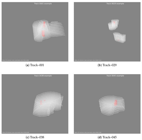
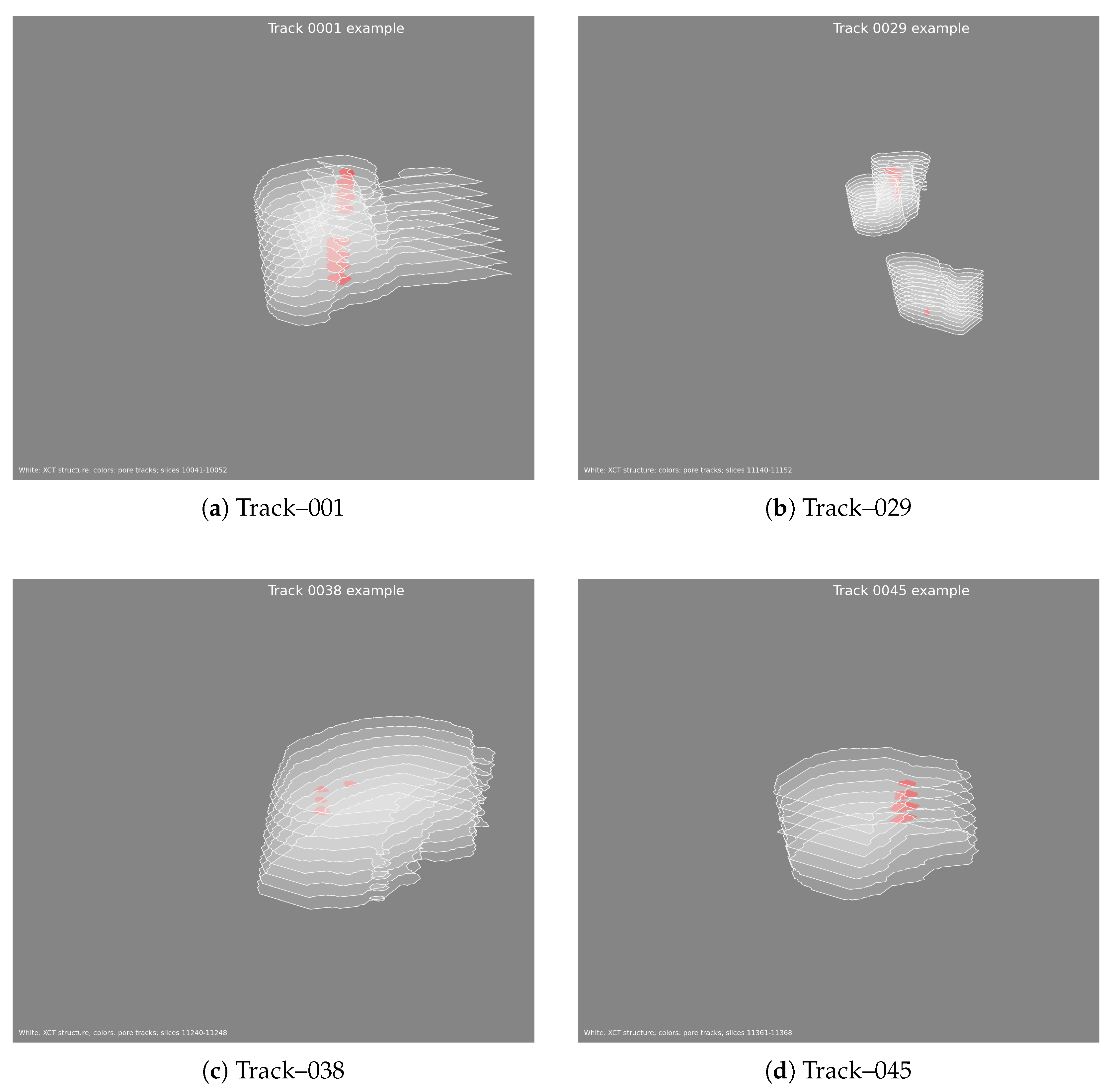
The 13 reviewed pore identities were organized into five groups for five-fold evaluation. Each fold used three groups for training, one for validation, and one for testing; keeping each group in one partition prevented slices or windows from the same tracks from crossing splits. Slices without reviewed identities were not treated as negative continuity annotations. Figure 1 shows representative reviewed tracks.

Figure 1. Examples of four individually annotated pore tracks from the XCT continuity dataset. Each panel shows one track across its ordered slices, with a small number of neighboring slices retained to provide structural context. The underlying XCT material is rendered as a translucent white stacked-slice surface and the selected pore track as a colored planar surface. The panels are qualitative dataset illustrations rather than physically exact three-dimensional reconstructions.

For the main association benchmark, detector proposals are intersected with reviewed pore instances. A proposal remains in the evaluated graph only when it has a valid correspondence to a reviewed instance, and only candidate edges whose two endpoints remain are preserved. This protocol isolates association errors from missed or spurious detections. It does not replace detector evaluation; candidate coverage is therefore reported separately and the association metrics are interpreted over the recoverable candidate set. Detector proposals were matched to reviewed pore instances independently on each slice. A proposal–annotation pair was eligible when its bounding-box IoU was at least 0.10 or its centroid distance was at most 25 pixels. Eligible pairs were ranked by $0.7\mathrm{IoU}+0.3\max (0,1-d_c/25)$ and greedily assigned one-to-one. Unmatched proposals were retained in the end-to-end audit but excluded from the conditional candidate–ground-truth intersection; unmatched annotations contributed to the node-coverage audit.

3.2. Continuity Annotations and Task Definition

A pore track is an ordered set of slice-level pore instances representing the same physical structure. For a source instance $v_i$ on slice $s_i$, a direct successor is the single annotated node that immediately follows it on the track. Different tracks can be close in space without being connected. A branch annotation records multiple track identities that coexist around a structural split, but each source retains only one directly annotated next node under the current source-choice convention. A terminal source has no annotated direct successor. Detector proposals on slices without continuity annotation are not reinterpreted as missing ground truth.

The single-direct-successor rule defines the present supervision and decoding task rather than imposing a physical assumption that pores cannot branch or merge. Multiple geometrically plausible outgoing relations may remain in the candidate graph, but each reviewed source contributes at most one positive direct-successor label, or a terminal decision when no successor is annotated; the source-choice decoder and global assignment enforce this feasibility constraint. When a physical branch, merge, or multiple connected subregions is represented by separate reviewed track identities, the corresponding direct-successor relations are evaluated within the same framework. The reported topology-related quantities therefore describe the reviewed local-connectivity decisions supported by the current annotation protocol.

Let $G=(V,E)$ be a directed candidate graph. Each node $v_i\in V$ has slice coordinate $s_i$ and feature vector ${\mathbf{x}}_i$. Each candidate edge $e_{ij}=(v_i,v_j)\in E$ points forward in the slice order and has feature vector ${\mathbf{r}}_{ij}$. The edge label $y_{ij}=1$ if $v_j$ is the annotated direct successor of $v_i$, and $y_{ij}=0$ otherwise. The model estimates a link probability $p_{ij}$ and a source-choice score over the available target edges and non-edge actions. The final output is a feasible selected edge set $E^{*}\subseteq E$, from which tracks and terminal behavior are reconstructed.

4. Proposed Method

4.1. Framework Overview

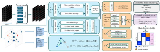
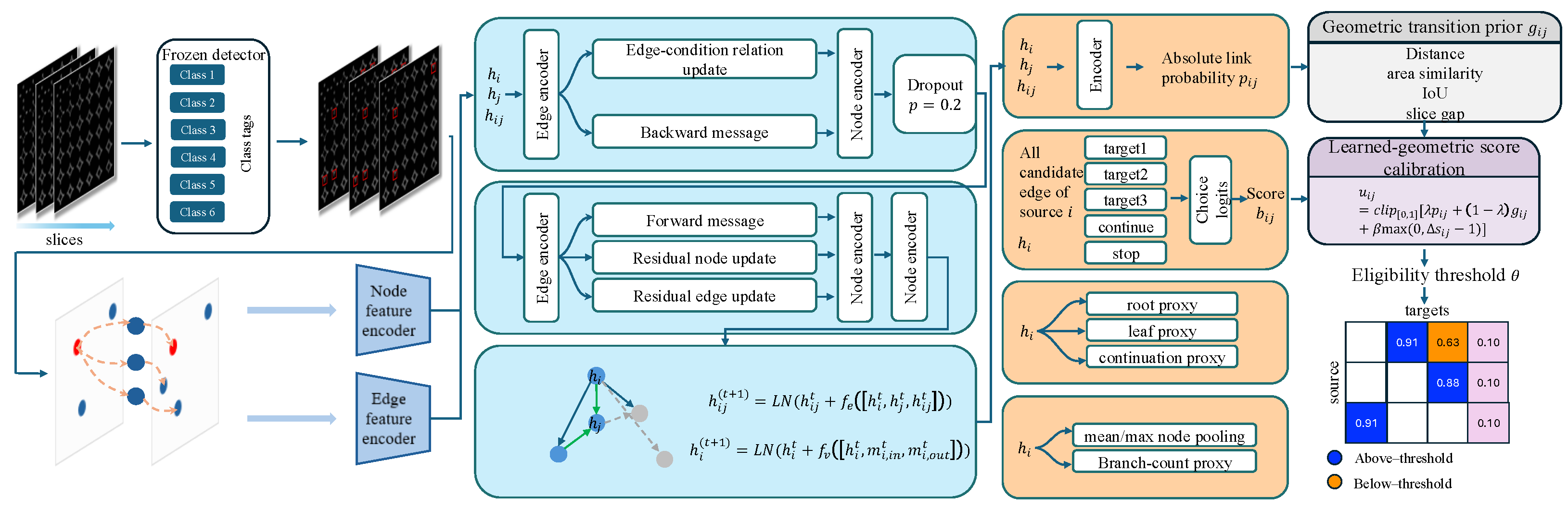
Figure 2 gives the detailed architecture of CAPG-Link and the information flow from the ordered XCT slices to the reconstructed pore tracks. The frozen six-class detector first converts the slice stack into pore candidates with class and structural metadata. The candidate builder then represents each pore proposal as a node and each admissible forward relation as a directed edge; separate node and edge encoders map these measurements into the hidden space used by the graph network. Within the blue message-passing blocks, edge states are updated from their incident nodes and edge context, while forward and backward messages allow each candidate to be evaluated against competing incoming and outgoing continuations. The orange prediction heads retain complementary views of the same representation: absolute edge probability estimates link plausibility; source-choice logits rank the alternatives for one source; and the root, leaf, continuation, and branch-count outputs provide topology-related auxiliary supervision.

Figure 2. Detailed architecture of CAPG-Link. The frozen six-class detector produces slice-wise pore candidates and structural context, which are converted into a directed candidate graph and encoded as node and edge representations. Residual bidirectional message passing updates these representations before the model predicts absolute link probabilities, source-relative choice logits, and topology-related proxy scores. A geometric transition prior is fused with the learned link probability; validation-selected calibration and the eligibility threshold then pass feasible candidates to the global one-to-one assignment that reconstructs pore tracks.

The six-class detector is frozen before continuity training. For every detected instance, the front end exports its confidence, bounding box, centroid, predicted class, slice identity, and available structure-unit metadata. Pore proposals become association nodes, while the remaining class and unit attributes supply local structural context. The graph builder considers only forward relations in slice order and retains edges that pass the frozen candidate rules. Consequently, the graph is directed and acyclic with respect to slice index.

During graph inference, separate encoders map node and edge measurements to a common hidden space. Three rounds of bidirectional message passing let one candidate edge interact with competing incoming and outgoing hypotheses. Multiple prediction heads then produce absolute node and edge probabilities, continuation and terminal proxies, and source-relative choice logits. The final Proposed system does not decode the raw neural edge probability alone. It combines that probability with a geometric transition probability and a gap prior; the fusion weights and acceptance threshold are selected on the validation graphs of each fold. A one-to-one global assignment then resolves conflicts among eligible edges. The selected directed edges are converted into pore tracks for evaluation.

All stages after the frozen detector are repeated independently in the five group-isolated folds. Model checkpoints, score-fusion parameters, and decision thresholds are chosen without consulting the corresponding test group. For the primary association experiment, the same workflow operates on candidate–ground-truth-intersection nodes and their induced edges; detector coverage is evaluated separately.

4.2. Slice-Wise Detection and Pore Candidate Projection

Let $I_s\in {\mathbb{R}}^{H\times W}$ denote the XCT image at slice s, where $H=W=1800$. The detector maps $I_s$ to a proposal set

$$D_s=\{d_i=(B_i,{\rho }_i,c_i,{\mathbf{m}}_i)\},$$

(1)

where $B_i=(x_i,y_i,w_i,h_i)$ is a bounding box, ${\rho }_i$ is detector confidence, $c_i$ is one of six front-end classes, and ${\mathbf{m}}_i$ contains the available structure identifiers. The center ${\mathbf{p}}_i=(x_i+w_i/2,y_i+h_i/2)$ and box area $A_i=w_i{h}_i$ are computed from $B_i$.

For detector operation, proposals are filtered and de-duplicated by the frozen front-end export procedure before graph construction. In the primary continuity benchmark, each exported proposal is matched to the manually reviewed pore annotations. We retain a node only when its [matched_gt_local_defect_id] is non-empty. If $V^{\prime }$ denotes the retained node set, the evaluated graph is the induced subgraph $G\left[V^{\prime }\right]$: no new edge is created after filtering, and an existing edge is retained only when both endpoints belong to $V^{\prime }$. This design guarantees that all compared association methods receive exactly the same recoverable pore instances and exactly the same candidate-edge opportunity set.

This projection defines the controlled association benchmark; detector coverage and unmatched proposals are evaluated separately in the end-to-end audit. Slice-level detector annotations and continuity annotations served different purposes: direct-successor supervision was defined only for the manually reviewed pore groups. Slices without reviewed continuity identities were not treated as negative links or as evidence that a pore terminated; unreviewed relations were excluded from the Link-F1 ground truth and their impact is reported through candidate coverage and the end-to-end audit.

4.3. Directed Candidate-Graph Construction

The graph builder organizes proposals by slice and creates a directed relation only from an earlier source node $v_i$ to a later target node $v_j$, so $s_j>s_i$. Candidate generation first considers adjacent slices and can retain a gap edge when the frozen graph export identifies a structurally compatible target across an intermediate slice. Spatial displacement, box overlap, area compatibility, unit consistency, and intermediate-candidate evidence are stored with each relation. Relations that are not emitted by this fixed builder never enter the learning or decoding stage.

For a graph window containing node set V and candidate edge set E, the positive-edge subset is

$$E^{+}=\{(i,j)\in E:\mathrm{id}\left(v_i\right)\to \mathrm{id}\left(v_j\right)\mathrm{is}\mathrm{an}\mathrm{annotated}\mathrm{direct}-\mathrm{successor}\mathrm{relation}\}.$$

(2)

All other emitted edges are local negatives. The exported training set uses complete reviewed graphs together with sliding windows of five selected slices, unit stride, a minimum of three slices, at least one positive node, and at least one positive edge. Window expansion increases the number of local training contexts while group isolation prevents a reviewed test group from entering the training or validation split.

Source-choice groups are derived after graph construction. For a positive source and the immediately following physical slice, all emitted candidate edges targeting that slice form the edge options; gap edges remain in the candidate graph and are scored by the edge head but are not part of this adjacent-slice source-choice group. A virtual [continue] option is included only when the continuation-target rule identifies an annotated successor beyond the currently visible candidate set, and a virtual [stop] option is included when at least one candidate edge or continuation option makes termination a competing decision. These virtual options are used by the source-choice loss and are not graph nodes or physical edges. Groups with fewer than two total options are excluded because they contain no ranking decision, and groups with more than one positive outgoing edge are excluded under the single-direct-successor convention. During primary inference, only eligible emitted edges enter thresholding and the global one-to-one assignment; its private dummy choice represents no selected successor, while virtual continue and stop logits provide source-level supervision rather than decoded physical links.

4.4. Node and Edge Representation

Each node uses a 16-dimensional feature vector. The features comprise proposal confidence; normalized centroid coordinates; normalized bounding-box width, height, and area; logarithmic aspect ratio; normalized slice position; indicators for an available structure-unit identifier and an available class-1 unit identifier; and a six-dimensional one-hot vector for the front-end class. Although association is evaluated only on pores, the class-context fields preserve information produced by the six-class front end.

Each directed candidate edge uses 20 features. Geometric continuity is represented by normalized slice gap, signed and absolute centroid displacement in both axes, normalized center distance, bounding-box intersection over union, and area similarity. Confidence compatibility is represented by source score, target score, score mean, and absolute score difference. Structural context comprises indicators for an identical structure unit, identical structure class, and identical class-1 unit. Gap context comprises whether a gap edge was used, normalized counts of intermediate candidates and same-unit intermediate candidates, and the maximum intermediate confidence with and without the same-unit restriction. These features distinguish a genuinely smooth continuation from a merely close candidate.

For clarity, representative geometric terms are

$$d_{ij}={\displaystyle \frac{{\parallel {\mathbf{c}}_j-{\mathbf{c}}_i\parallel }_2}{D}},q_{ij}={\displaystyle \frac{\min (A_i,A_j)}{\max (A_i,A_j)}},o_{ij}={\displaystyle \frac{|B_i\cap B_j|}{|B_i\cup B_j|}},$$

(3)

where $\mathbf{c}$, A, and B denote centroid, bounding-box area, and bounding box, respectively, and D is the normalization scale used by graph export. The full feature vector is read from the frozen graph representation rather than recomputed differently for individual comparison methods.

Table 3 groups the model inputs by role. The explicit separation supports the inference-time sensitivity analysis, which masks selected cross-slice edge measurements while keeping the evaluated candidate nodes fixed.

Table 3. Frozen node and edge features used by the continuity graph.

Group	Features
Node confidence and geometry	score; normalized center x/y; normalized box width, height, and area; log aspect ratio; normalized slice position
Node structural context	structure-unit availability; class-1-unit availability; six-class one-hot indicators
Edge displacement and shape	normalized slice gap; signed and absolute x/y displacement; center distance; box IoU; area similarity
Edge confidence context	source score; target score; mean score; absolute score difference
Edge structural context	same structure unit; same structure class; same class-1 unit
Gap/intermediate context	gap-edge flag; normalized intermediate-candidate counts; same-unit counts; maximum intermediate scores

For the masking analysis, 11 of the 20 edge dimensions were designated as continuity features: normalized slice gap; signed and absolute centroid displacement in both axes; normalized center distance; the gap-edge indicator; normalized counts of intermediate candidates and same-unit intermediate candidates; and maximum intermediate confidence with and without the same-unit restriction. Bounding-box IoU, area similarity, the four confidence features, and the three structural-context indicators were retained.

4.5. Continuity-Aware Graph Network

CAPG-Link maps node and edge features into 128-dimensional hidden representations with separate multilayer perceptrons. It then applies three residual message-passing steps. At step t, the representation of edge $(i,j)$ is updated from the current source, target, and edge states:

$${\mathbf{h}}_{ij}^{t+1}=\mathrm{LN}\left({\mathbf{h}}_{ij}^t+f_e^t\left([{\mathbf{h}}_i^t,{\mathbf{h}}_j^t,{\mathbf{h}}_{ij}^t]\right)\right).$$

(4)

Two directed message functions propagate information forward and backward. Incoming forward messages and outgoing backward messages are summed at each node, after which a residual node update is applied:

$${\mathbf{h}}_i^{t+1}=\mathrm{LN}\left({\mathbf{h}}_i^t+f_v^t\left([{\mathbf{h}}_i^t,{\mathbf{m}}_{i,\mathrm{in}}^t,{\mathbf{m}}_{i,\mathrm{out}}^t]\right)\right).$$

(5)

Layer normalization and dropout with probability 0.20 are used in the network. Bidirectional aggregation is useful here because an edge should be assessed not only by its local geometry but also by competing incoming and outgoing continuations.

The updated node states feed node, root-proxy, leaf-proxy, continuation, and stop heads. An edge head receives the updated source state, target state, edge state, and five role logits consisting of source root, source leaf, source continuation, target root, and target leaf scores. A parallel edge-choice head produces source-relative edge logits. The root and leaf outputs are treated as terminal-behavior proxies; this paper does not claim a broadly independent stop-classification benchmark.

More explicitly, let ${\mathsf{\ell }}_i^r$, ${\mathsf{\ell }}_i^l$, and ${\mathsf{\ell }}_i^c$ denote the root-proxy, leaf-proxy, and continuation logits of node i. The edge-classification input is

$${\mathbf{g}}_{ij}=[{\mathbf{h}}_i^T,{\mathbf{h}}_j^T,{\mathbf{h}}_{ij}^T,{\mathsf{\ell }}_i^r,{\mathsf{\ell }}_i^l,{\mathsf{\ell }}_i^c,{\mathsf{\ell }}_j^r,{\mathsf{\ell }}_j^l],$$

(6)

and separate multilayer heads map ${\mathbf{g}}_{ij}$ to an absolute edge logit $a_{ij}$ and a source-choice logit $b_{ij}$. The absolute probability $p_{ij}=\sigma \left(a_{ij}\right)$ answers whether an edge is plausible in isolation. The choice logit answers a different question: whether that edge should be preferred over the other options available to the same source. Keeping both heads preserves calibrated edge eligibility while directly training ambiguous local rankings.

The graph-level branch-count proxy uses the concatenation of mean and maximum node embeddings. This auxiliary head encourages the shared representation to retain graph-scale topology information, but branch count is not used to override the direct-successor constraint at decoding time. The distinction prevents the term branch from being misread as unrestricted one-to-many edge selection from a single annotated source.

4.6. Multi-Task and Source-Choice Supervision

Node and edge targets use weighted binary cross entropy. Root, leaf, and continuation auxiliary terms provide topology-related supervision, and the graph-level branch-count head predicts a positive branch-count proxy from concatenated mean and maximum graph embeddings. The distinctive source-choice term groups all decisions available to one source. Depending on the annotation and candidate set, the correct option is a target edge, a continue action, or a stop action. Cross entropy over this local option set encourages the model to rank the annotated decision above its direct competitors rather than scoring every edge independently.

The total objective is

$$\mathcal{L}={\lambda }_n{\mathcal{L}}_n+{\lambda }_e{\mathcal{L}}_e+{\lambda }_r{\mathcal{L}}_r+{\lambda }_l{\mathcal{L}}_l+{\lambda }_c{\mathcal{L}}_c+{\lambda }_b{\mathcal{L}}_b+{\lambda }_{sc}{\mathcal{L}}_{sc}.$$

(7)

In the full CAPG-Link configuration, ${\lambda }_c=1.25$ and ${\lambda }_{sc}=1.25$. Source-choice groups are additionally weighted by 0.5, 3.0, and 2.0 for edge, continue, and stop targets, respectively. This weighting emphasizes non-edge decisions without discarding absolute edge supervision. The validation monitor is source-choice non-edge macro recall, and early stopping begins only after the configured minimum number of epochs; no test fold is used for this selection.

For a source-choice group $C_i$, define its ordered options as the candidate edge logits, followed when applicable by the continuation and stop logits:

$${\mathbf{o}}_i=[\{b_{ij}:(i,j)\in C_i\},{\mathsf{\ell }}_i^c\left(\mathrm{optional}\right),{\mathsf{\ell }}_i^s\left(\mathrm{optional}\right)].$$

(8)

If $k_i$ is the annotated option index, its loss is

$${\mathcal{L}}_{sc}^{\left(i\right)}=-w_{t_i}\log {\displaystyle \frac{\exp \left(o_{i,k_i}\right)}{{\sum }_k\exp \left(o_{i,k}\right)}},$$

(9)

where $t_i\in \{\mathrm{edge},\mathrm{continue},\mathrm{stop}\}$ and $w_{t_i}$ is the group-type weight. The implementation normalizes the sum of weighted group losses by the sum of group weights. This source-relative objective supplies hard local negatives naturally: every incorrect target in the same option set competes directly with the annotated successor.

Checkpoint selection monitors the macro average of validation recall for continue and stop groups. This criterion was chosen because an edge-only monitor can favor a model that connects every eligible source but fails to recognize non-edge actions. For the full CAPG-Link configuration, early stopping uses a patience of 16 epochs after a minimum of 10 epochs. The held-out test graphs are evaluated only after this training decision has been frozen.

4.7. Validation-Selected Score Fusion

The main proposed system combines the neural continuity probability with an explicit geometric transition prior before global assignment. For candidate edge $(i,j)$, the geometric cost is

$$C_{ij}={\displaystyle \frac{d_{ij}^{\mathrm{pix}}}{{\tau }_d}}+{\alpha }_A(1-q_{ij})+{\alpha }_I(1-o_{ij})+{\alpha }_G\max (0,\Delta s_{ij}-1),$$

(10)

where $d_{ij}^{\mathrm{pix}}$ is center distance in pixels, $q_{ij}$ is area similarity, $o_{ij}$ is bounding-box IoU, $\Delta s_{ij}$ is the slice gap, and ${\tau }_d$, ${\alpha }_A$, ${\alpha }_I$, and ${\alpha }_G$ are the geometry parameters frozen from the validation-selected classical configuration. The corresponding geometric probability is $g_{ij}=\exp (-C_{ij})$. Edge-feature distances are normalized by the spatial extent of the exported graph, with the graph diagonal used for center distance, whereas this geometric cost uses centroid distance in pixels divided by a validation-selected distance scale. Specifically, ${\tau }_d\in \{5,10,20\}$ pixels, ${\alpha }_A,{\alpha }_I,{\alpha }_G\in \{0,0.5\}$, and the rejection threshold was selected from $\{0.5,1,2,4\}$ using validation graphs only. Candidate construction was fixed before training, with maximum slice gap 2, maximum centroid distance 48 pixels, and minimum area similarity 0.05; these parameters were not learned from test folds.

Let $p_{ij}$ be the absolute edge probability predicted by CAPG-Link. The fused score used by the final decoder is

$$u_{ij}={\mathrm{clip}}_{[0,1]}\left[\lambda p_{ij}+(1-\lambda )g_{ij}+\beta \max (0,\Delta s_{ij}-1)\right].$$

(11)

The learned weight $\lambda \in \{0,0.25,0.5,0.75,1\}$, gap adjustment $\beta \in \{0,0.05,0.10,0.20\}$, and eligibility threshold $\theta \in \{0.10,0.15,\dots ,0.95\}$ form a grid of 360 configurations. For each fold, the configuration maximizing Link F1 on full validation graphs is selected. Validation ties are resolved by preferring more learned evidence, then a smaller gap adjustment, and finally a more conservative (higher) threshold. The chosen configuration is applied once to the corresponding test fold.

This fusion has a specific interpretation. Geometry provides a stable inductive prior for easy links, whereas the graph probability incorporates competition and contextual continuity. The term controlled by $\beta$ is a validation-selected adjustment for an already emitted gap candidate, not a mechanism that creates a missing edge. An adjacent-slice edge ($\Delta s_{ij}=1$) receives no adjustment, whereas the only permitted gap edge ($\Delta s_{ij}=2$) receives $\beta$; candidate construction limits $\Delta s_{ij}$ to at most 2, so the term cannot encourage arbitrarily long links. Such a candidate must still pass the fixed distance and area-similarity gates, exceed the selected eligibility threshold, and compete in the global one-to-one assignment. This post-model adjustment is distinct from the learned gap-related edge features, which are inputs to CAPG-Link before score fusion. Although nonzero values were included in the validation grid to compensate for a possible score bias against a one-slice interruption, all five folds selected $\beta =0$; consequently, the reported primary results do not depend on an added gap score. Because all fusion parameters are selected without test labels, their use does not change the held-out evaluation protocol.

4.8. Global One-to-One Decoding

Only edges with $u_{ij}\ge \theta$ enter the assignment problem. Let S and T be the unique source and target identities among these eligible edges. We construct a rectangular cost matrix with one row per source, one column per target, and one private dummy column per source. A real source–target entry has cost $-u_{ij}$; a missing edge is assigned a large invalid cost. The private dummy entry has cost $-\theta$ and represents selecting no outgoing link for that source. The linear-sum assignment algorithm minimizes this matrix cost.

Equivalently, the selected variables solve

$$\underset{\mathbf{z}}{\max }\sum _{(i,j)\in E_{\theta }}{u}_{ij}{z}_{ij}+\theta \sum _{i\in S}{z}_{i⌀},$$

(12)

subject to

$$\sum _{j:(i,j)\in E_{\theta }}{z}_{ij}+z_{i⌀}=1,\sum _{i:(i,j)\in E_{\theta }}{z}_{ij}\le 1,$$

(13)

where $E_{\theta }$ is the eligible edge set and $z_{i⌀}$ is the private no-link choice. Thus every source either selects one eligible successor or terminates, and no target can be claimed by two sources. The dummy cost also ensures that an edge must offer at least threshold-level utility to displace the no-link option.

The global step serves two purposes. First, it prevents independently high-scoring edges from producing duplicate predecessors or successors. Second, it separates evidence estimation from structural feasibility: the learned CAPG-Link score and the geometric prior estimate transition utility, while the assignment layer guarantees consistency with the single-direct-successor annotation convention. Classical Hungarian and min-cost-flow baselines receive the same nodes and candidate edges; their difference lies in transition scoring and decoding, not in access to easier candidate graphs.

4.9. Track Reconstruction and Output Semantics

After assignment, rejected edge probabilities are set to zero in the shared prediction serializer and selected edges are exported with the retained nodes. Since all graph edges point forward in slice order and in/out degree is at most one after decoding, each connected component forms a directed chain. A node without a selected predecessor initializes a reconstructed track, and traversal continues until a node selects the private no-link option or has no eligible successor.

The benchmark’s reviewed branch structures are represented by distinct track/source identities whose direct-successor chains coexist in the same local region. The decoder does not manufacture an unrestricted one-to-many branch from a single source. Likewise, a track ending at the boundary of the annotated graph is not automatically interpreted as a physical pore termination beyond the observed range. These output semantics are why the paper reports terminal root/leaf behavior as proxies and avoids claiming a universally validated stop-vs-edge classifier.

The fold-wise training and held-out inference procedure is summarized below.

Procedure 1: Fold-wise continuity-aware pore association.

• Freeze the six-class detector and export slice-wise proposals and metadata.
• Build directed candidate graphs; derive node/edge labels and source-choice option sets.
• Train the CAPG-Link graph network with node, edge, topology-proxy, continuation, and source-choice losses.
• Select the checkpoint using validation source-choice non-edge macro recall.
• Infer validation edge probabilities and search $(\lambda ,\beta ,\theta )$ using validation Link F1 only.
• Infer test edge probabilities; fuse learned and geometric scores using the frozen validation configuration.
• Apply global one-to-one assignment with one private no-link dummy per source.
• Serialize selected nodes/edges, reconstruct directed tracks, and evaluate against projected test GT.

4.10. Implementation Scope

All feature definitions, candidate edges, fold assignments, and labels are loaded from frozen graph exports. Node and edge encoders use a hidden width of 128, the network uses three message-passing steps and dropout 0.20, and all normalization layers in the full CAPG-Link configuration are enabled. Model selection uses validation groups only; final fusion searches 360 validation configurations per fold. The oracle-intersection evaluation disables virtual-tail completion so that the predicted test links are restricted to the frozen induced candidate graph.

All compared methods used the same group-isolated folds, frozen candidate nodes and edges, test samples, and evaluation implementation. Hyperparameters and decision thresholds were selected using validation graphs only, without access to test labels. The classical methods shared the geometric cost $C_{ij}=d_{ij}/D+{\lambda }_A(1-q_{ij})+{\lambda }_I(1-o_{ij})+{\lambda }_G(\Delta s_{ij}-1)$, with its weights and rejection threshold selected from a common validation grid; they did not use CAPG-Link logits or hidden representations. Hungarian/LAP and min-cost flow allowed an unmatched source and enforced one-to-one source–target associations. The learning-based comparisons were adapted to the same graph input and fold protocol, and all final predictions were scored by the same evaluator. This common protocol isolates the association rule or learned linker as the principal difference between methods. For the Trackastra and MOTIP-style comparisons, the common frozen candidate graph replaced the original detection and candidate-generation input while their association mechanisms were evaluated under the same fold protocol. The nearest-neighbor baseline selected the lowest-cost eligible outgoing edge for each source and resolved target collisions by retaining the lower-cost association; sources without an eligible edge remained unmatched.

We distinguish two evaluation scopes. The conditional association benchmark evaluates link selection on the frozen candidate–ground-truth intersection, thereby isolating association quality when matched nodes are available. The end-to-end audit retains unmatched detector proposals and includes errors from node availability, candidate generation, link scoring, and decoding. Consequently, the conditional Link F1 is not interpreted as full-volume detector-to-track performance; the candidate-coverage analysis quantifies the upstream recoverability gap between the two scopes.

The primary benchmark retains only nodes with a non-empty matched ground-truth local defect identifier and evaluates the induced candidate edges. The five-fold result therefore measures association quality conditional on available candidates, while detector coverage is reported separately.

Candidate coverage was evaluated against the original, unprojected test annotations. Node coverage is the fraction of annotated nodes matched by a candidate, $C_{\mathrm{node}}=|V_{\mathrm{GT}}\cap V_{\mathrm{cand}}|/|V_{\mathrm{GT}}|$. Candidate-link coverage is the fraction of annotated directed links explicitly present in the frozen graph, $C_{\mathrm{link}}=|E_{\mathrm{GT}}\cap E_{\mathrm{cand}}|/|E_{\mathrm{GT}}|$; merely covering both endpoint nodes is insufficient. Assuming oracle selection of all represented links without false positives, the corresponding Link F1 ceiling is $2C_{\mathrm{link}}/(1+C_{\mathrm{link}})$.

4.11. Metrics

For links, a true positive (TP) is a predicted directed edge whose source and target form one reviewed direct-successor pair. A false positive (FP) is a predicted edge that is absent from the reviewed edge set, including a wrong target or an edge incident to an unmatched node; a false negative (FN) is a reviewed directed edge that is not predicted. In the conditional benchmark, ground-truth nodes without a matched candidate are excluded by the node projection, but a reviewed edge still contributes to FN when both endpoints remain and the candidate graph lacks that directed edge. The end-to-end audit additionally includes errors caused by unmatched or missing nodes. Link precision, recall, and F1 are

$$P={\displaystyle \frac{TP}{TP+FP}},R={\displaystyle \frac{TP}{TP+FN}},F1={\displaystyle \frac{2PR}{P+R}}={\displaystyle \frac{2TP}{2TP+FP+FN}}.$$

(14)

Node F1 uses the analogous counts for predicted and reviewed pore instances. Path-reachability F1 compares ordered source–descendant reachability pairs after mapping predicted nodes to reviewed instances, rather than counting only immediate edges. Root and leaf scores compare the reviewed and predicted terminal-node sets and are reported as terminal-behavior proxies. Branch-count accuracy is the fraction of evaluated graphs whose predicted and reviewed branch-count proxies agree exactly; it is not an unrestricted branch-reconstruction metric under the single-direct-successor convention.

Unless stated otherwise, Link and node metrics are micro-aggregated by summing TP, FP, and FN over the graphs in a fold and then computing the metric. Reported five-fold means and standard deviations are computed from the five fold-level metric values; they are not volume-level confidence intervals. Coverage metrics use their explicitly stated node, directed-edge, and complete-track denominators.

5. Results

5.1. Front-End Audit and Candidate Coverage

The six-class detector achieved AP 0.789, AP50 0.861, AP75 0.846, precision 0.808, recall 0.861, F1 0.834, and AR100 0.928 on 159 held-out XCT images (Table 4).

Table 4. Six-class front-end audit.

Scope	Metric	Value
Overall	AP	0.789
Overall	AP50	0.861
Overall	AP75	0.846
Overall	Precision	0.808
Overall	Recall	0.861
Overall	F1	0.834
Overall	AR100	0.928
Labels 1–6	AP range	0.724–0.867

Table 5 quantifies the candidate-graph ceiling before link scoring and decoding. Micro-aggregated over the five test folds, the graph covered 61/64 annotated nodes and explicitly represented 47/51 directed links, yielding an oracle Link F1 ceiling of 95.92%. Node coverage alone was insufficient: in Fold 1 both endpoints of the slice-10046-to-10049 gap link were present, but the directed candidate edge was absent. At the stricter track level, all nodes and links were represented for 9 of 13 annotated tracks.

Table 5. Coverage ceiling of the frozen candidate graph on the annotated test folds.

Test Fold	GT Nodes	Node Coverage	GT Links	Candidate-Link Coverage	Oracle Link F1 Ceiling
Fold 1	8	8/8 (100.00%)	7	6/7 (85.71%)	92.31%
Fold 2	7	7/7 (100.00%)	6	6/6 (100.00%)	100.00%
Fold 3	20	19/20 (95.00%)	14	13/14 (92.86%)	96.30%
Fold 4	23	22/23 (95.65%)	20	19/20 (95.00%)	97.44%
Fold 5	6	5/6 (83.33%)	4	3/4 (75.00%)	85.71%
Micro total	64	61/64 (95.31%)	51	47/51 (92.16%)	95.92%

These values describe the reviewed continuity subset used for the conditional benchmark.

5.2. End-to-End Detector-to-Track Audit

The fold test exports also retain unmatched detector proposals, allowing an end-to-end audit in which node availability is not conditioned on a ground-truth intersection. Across the five held-out groups, CAPG-Link achieved mean node F1 of 0.9246, mean link F1 of 0.9509, link precision of 1.0000, link recall of 0.9114, and path-reachability F1 of 0.8999. The corresponding fold values are reported in Table 6. These values are lower than the conditional association result because missed or unmatched pore proposals cannot be recovered by the linker. The end-to-end audit therefore reports the complete detector-to-linker behavior, while the conditional protocol remains useful for isolating association quality when the correct node is available.

Table 6. End-to-end detector-to-track audit for CAPG-Link (unmatched detector proposals retained).

Metric	Mean	Fold 1	Fold 2	Fold 3	Fold 4	Fold 5
Node F1	0.9246	1.0000	1.0000	1.0000	0.9565	0.6667
Link precision	1.0000	1.0000	1.0000	1.0000	1.0000	1.0000
Link recall	0.9114	0.8571	1.0000	1.0000	0.9500	0.7500
Link F1	0.9509	0.9231	1.0000	1.0000	0.9744	0.8571
Path reachability F1	0.8999	0.6000	1.0000	1.0000	0.9762	0.9231

5.3. External Comparison

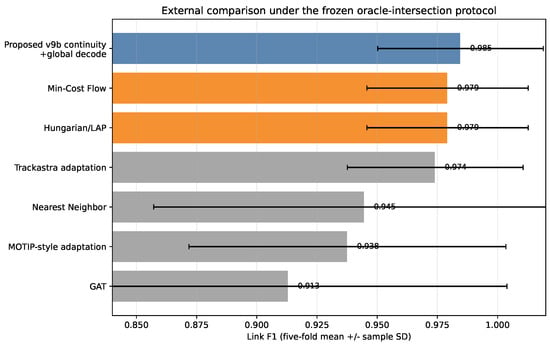
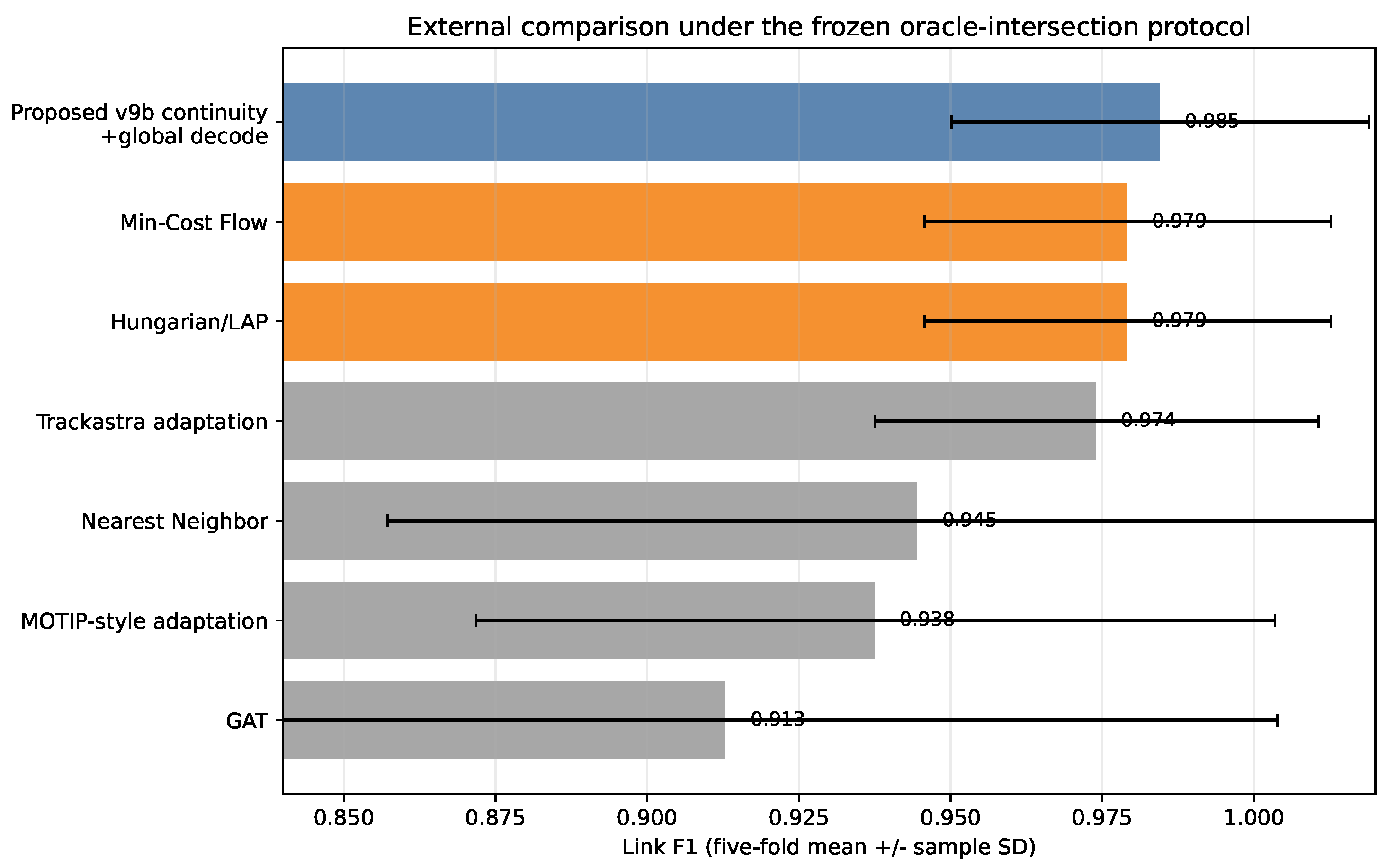
The comparison includes CAPG-Link (this work), Hungarian/linear-assignment (LAP) matching [21,22], min-cost flow [23], a Trackastra adaptation, an in-house nearest-neighbor matching baseline, a MOTIP-style adaptation [30], and a graph-attention-network (GAT) baseline [27]. The nearest-neighbor row is a simple geometric reference implementation and is not presented as a reproduction of a named published tracker. The proposed method obtained mean Link F1 $0.9846\pm 0.0344$ across folds, the highest observed mean (Table 7). Hungarian/LAP and min-cost flow each obtained $0.9792\pm 0.0335$, Trackastra adaptation $0.9741\pm 0.0365$, nearest neighbor $0.9446\pm 0.0874$, MOTIP-style adaptation $0.9377\pm 0.0658$, and GAT $0.9130\pm 0.0909$. The proposed method won one fold and tied four against Hungarian and min-cost flow, with no fold-level loss. Figure 3 presents the same comparison graphically with fold-level standard-deviation bars, making the small margin over assignment baselines and the larger gap to local or adapted learning baselines visible at a glance.

Table 7. Main five-fold external comparison (Link F1). Literature-derived baselines are cited in the text; the nearest-neighbor row is an in-house geometric baseline.

Method	Mean ± SD	F1-1	F1-2	F1-3	F1-4	F1-5
CAPG-Link	0.9846 ± 0.0344	0.9231	1.0000	1.0000	0.9744	1.0000
Hungarian/LAP	0.9792 ± 0.0335	0.9231	1.0000	1.0000	0.9474	1.0000
Min-cost flow	0.9792 ± 0.0335	0.9231	1.0000	1.0000	0.9474	1.0000
Trackastra adaptation	0.9741 ± 0.0365	0.9231	1.0000	1.0000	0.9217	1.0000
Nearest neighbor	0.9446 ± 0.0874	0.9231	1.0000	0.8000	0.9474	1.0000
MOTIP adaptation	0.9377 ± 0.0658	0.9231	1.0000	0.9231	0.8165	1.0000
GAT	0.9130 ± 0.0909	0.9231	0.8000	1.0000	0.8165	1.0000

Figure 3. Five-fold external comparison under the common candidate-graph protocol. Bars show mean Link F1 and sample standard deviation across folds.

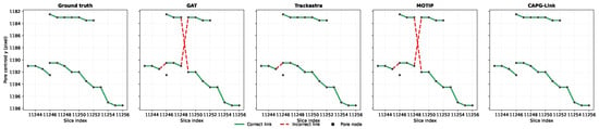
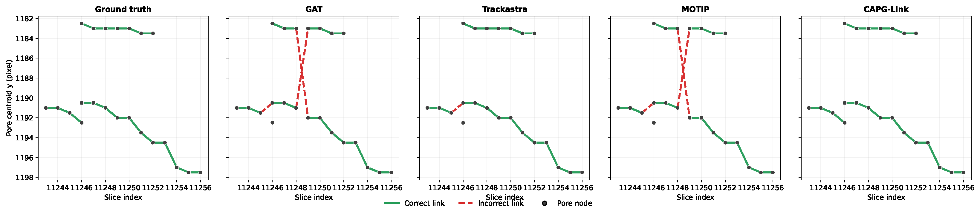
To complement the aggregate scores, Figure 4 visualizes the final association decisions on the same fold-04 candidate graph. This qualitative comparison is restricted to independently trained deep-learning models: GAT, the Trackastra adaptation, the MOTIP-style adaptation, and CAPG-Link. The ground-truth panel is shown first, followed by the four model outputs, with identical node coordinates and slice axes in every panel. Green solid segments denote links that agree with the reviewed ground truth, whereas red dashed segments denote incorrect selected links. Thus, the figure exposes the type of error that is hidden by a single fold-level F1 value, including competing-target choices and cross-track connections.

Figure 4. Qualitative comparison of deep-learning association models on the same fold-04 candidate graph. From left to right: reviewed ground truth, GAT, Trackastra adaptation, MOTIP adaptation, and CAPG-Link. All panels share the same pore nodes and coordinate system. Green solid links are correct selections and red dashed links are incorrect selections.

5.4. Runtime and Resource Cost

We measured association and decoding cost on the same five frozen oracle-intersection test graphs used for the accuracy comparison. Each graph was warmed up before repeated timing, and the reported time is the mean of the per-graph medians. Learned methods ran on an NVIDIA RTX 3090 GPU, whereas the classical decoders ran on CPU (Table 8). The five graphs contained 64 nodes and 121 candidate edges in total (mean 12.8 nodes and 24.2 edges; maximum 23 nodes and 70 edges). Detector inference, candidate generation, graph construction, disk I/O, and complete 1800-slice volume processing were not included in this association-only comparison.

Table 8. Association and decoding runtime on the frozen candidate graphs.

Method	Parameters	Device	Time (ms/Graph)	Peak Memory (MB)
CAPG-Link	1,045,256	RTX 3090 GPU	2.630	13.2–13.4
GAT	15,105	RTX 3090 GPU	3.331	9–10
MOTIP-style	88,706	RTX 3090 GPU	0.869	9–10
Trackastra adaptation	94,849	RTX 3090 GPU	0.656	9–10
Nearest neighbor	N/A	CPU	0.025	not sampled
Hungarian/LAP	N/A	CPU	0.037	not sampled
Min-cost flow	N/A	CPU	0.668	not sampled

The measurements used Python 3.10.19, PyTorch 2.1.0 with CUDA 12.1, and an RTX 3090 with 24 GB memory. The CAPG-Link linker checkpoint contains 1,045,256 parameters (4.1 MB); the reported classical methods have no trainable parameters.

5.5. Multi-Candidate Ambiguity Analysis

To quantify a difficult case that is defined directly by the frozen candidate graph, we identified an ambiguous source as a source node with at least two forward candidate successors. This criterion is independent of model predictions and captures competing successor hypotheses without introducing new dataset labels. Across the five folds, 41 ambiguous sources were identified; 39 had an annotated successor and were therefore evaluable for positive-link recall. On this subset, CAPG-Link recovered all 39 evaluable links without a false positive (Link F1 $=1.0000$), whereas Hungarian/LAP and min-cost flow each missed one link (Link F1 $=0.9870$). Trackastra, nearest neighbor, GAT, and MOTIP-style adaptation obtained Link F1 values of 0.9744, 0.9211, 0.9091, and 0.8974, respectively (Table 9).

Table 9. Performance on objectively defined multi-candidate ambiguous sources. The subset contains 41 sources, of which 39 have an evaluable ground-truth successor.

Method	TP	FP	FN	Precision	Recall	Link F1
CAPG-Link	39	0	0	1.0000	1.0000	1.0000
Hungarian/LAP	38	0	1	1.0000	0.9744	0.9870
Min-cost flow	38	0	1	1.0000	0.9744	0.9870
Trackastra adaptation	38	1	1	0.9744	0.9744	0.9744
Nearest neighbor	35	2	4	0.9459	0.8974	0.9211
GAT	35	3	4	0.9211	0.8974	0.9091
MOTIP-style adaptation	35	4	4	0.8974	0.8974	0.8974

The observed difference from the assignment baselines was concentrated in one Fold-4 connection. Branch, boundary, small-pore, and artifact categories were outside the original node-level annotation protocol and are, therefore, represented through traceable qualitative examples.

5.6. Visual Audit of Difficult Associations

To complement the aggregate ambiguity analysis, we inspected representative cases directly in the original slice masks. Figure 5 shows the Fold-4 relation from slice 11253 to slice 11254, where two successor candidates are present: CAPG-Link selects the reviewed link and the assignment baselines select neither the reviewed relation nor the same successor. The strip displays the surrounding slices 11250–11256 and retains the original pore-pixel extents. The three panels share one color encoding: green pixel regions belong to the reviewed track and red ones do not, while a dashed red arrow marks a relation that is not the reviewed link (a competing baseline choice, or a reviewed relation with no candidate edge).

Figure 5. Representative Fold-4 multi-candidate case. The slice strip uses the original pore-pixel regions and provides context around the reviewed relation from slice 11253 to slice 11254. The red region is the competing candidate at slice 11255.

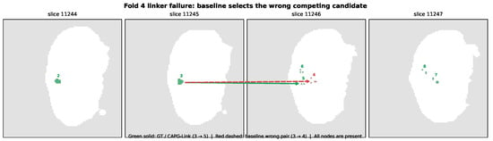
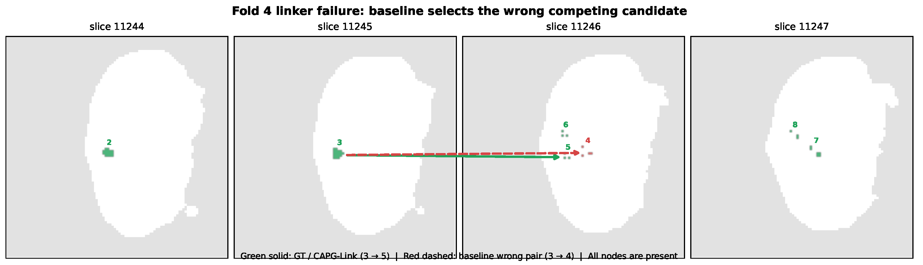
Figure 6 illustrates a separate linker-level failure: all relevant nodes and candidate edges are present, but a baseline selects a competing target while CAPG-Link selects the reviewed successor. In contrast, the Fold-1 diagnostic in Figure 7 contains a reviewed gap relation that is absent from the frozen candidate graph; this case isolates candidate generation from downstream linker selection. The branch example is a qualitative pipeline-validity pilot based on confirmed ground-truth boxes.

Figure 6. Fold-4 linker-level failure strip. The ground-truth and CAPG-Link successor are present in the candidate graph, while the baseline selects a competing target. The red region is the competing candidate, instance 4.

Figure 7. Fold-1 candidate-generation diagnostic. The reviewed gap relation is not emitted by the frozen candidate graph, so the case cannot be recovered by any downstream linker. Both endpoints belong to the same reviewed track, so all regions are green; the dashed arrow marks the reviewed relation that has no candidate edge.

5.7. Mechanism Evidence and Internal Ablation

In the internal comparison, the CAPG-Link variant without graph message passing, an intermediate CAPG-Link configuration with fixed score calibration, and the full CAPG-Link obtained mean Link F1 values of 0.9568, 0.9509, and 0.9846, respectively (Table 10). This comparison is intended to show the contribution of learned graph reasoning and validation-selected calibration; the intermediate configuration is not a single-module removal.

Table 10. Internal CAPG-Link configuration comparison.

Variant	Mean	F1-1	F1-2	F1-3	F1-4	F1-5
CAPG-Link without graph message passing	0.9568	0.9231	1.0000	0.9167	0.9444	1.0000
CAPG-Link with fixed score calibration	0.9509	0.9231	1.0000	1.0000	0.9744	0.8571
CAPG-Link (full)	0.9846	0.9231	1.0000	1.0000	0.9744	1.0000

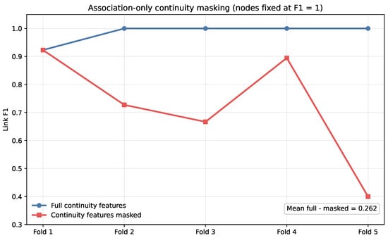
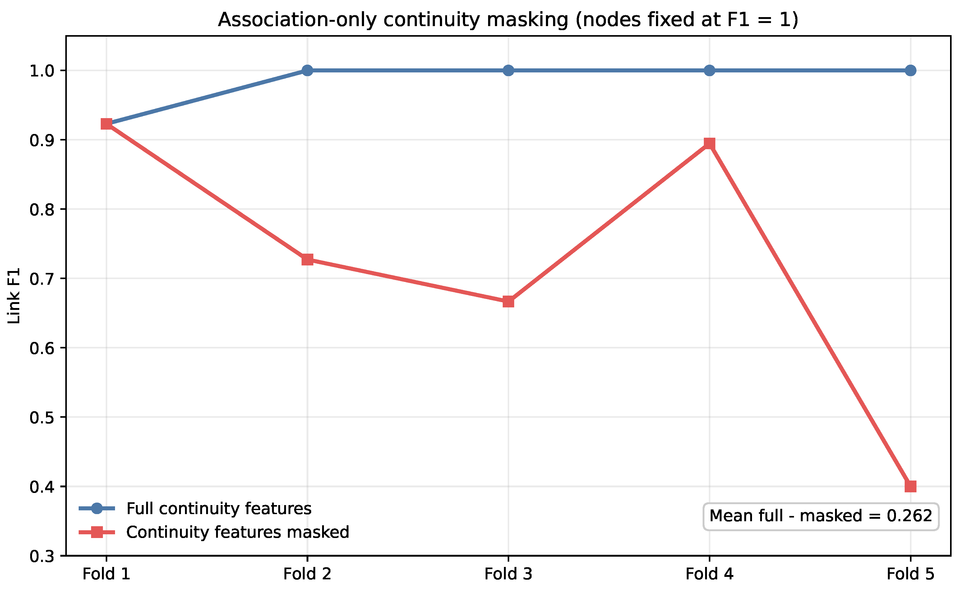
In the association-only masking experiment, the five checkpoints trained with the complete edge representation were retained. The 11 designated continuity dimensions were set directly to 0.0 in the validation and test graph inputs; no input dimension was deleted or replaced by a training-set mean. Node features, candidate nodes, candidate edges, and feature-vector dimensionality remained unchanged. The edge threshold was reselected on the masked validation graphs before evaluation on the masked test graphs. The resulting mean Link F1 was 0.7224, compared with 0.9846 for the unmasked condition; Node F1 remained 1.0 in every fold. Table 11 reports the fold-level comparison.

Table 11. Association-only continuity masking. The evaluated node set was fixed in both conditions.

Fold	Full	Masked	Drop	Node F1
fold01	0.9231	0.9231	0.0000	1.0000
fold02	1.0000	0.7273	0.2727	1.0000
fold03	1.0000	0.6667	0.3333	1.0000
fold04	1.0000	0.8947	0.1053	1.0000
fold05	1.0000	0.4000	0.6000	1.0000
Mean	0.9846	0.7224	0.2623	1.0000

The reduction was largest in fold05, followed by folds03, 02, and 04, while fold01 showed no additional decrease (Figure 8). In fold01, the ground-truth gap link from slice 10046 to slice 10049 was absent from the frozen candidate graph, so masking could not further affect that unrecoverable relation. Group-wise masks were also applied using the same protocol (Table 12). Displacement/distance produced the largest mean Link F1 reduction (0.0336), followed by intermediate-candidate context (0.0182) and slice-gap context (0.0154). Joint masking produced a substantially larger reduction, indicating sensitivity to the combined continuity representation.

Figure 8. Association-only continuity masking. Full and masked conditions are compared fold by fold while the evaluated node set is held fixed.

Table 12. Group-wise continuity masking. Drops are relative to the full-feature mean Link F1 of 0.9846.

Masked Feature Group	Mean Link P	Mean Link R	Mean Link F1	Drop
Displacement/distance	0.9846	0.9227	0.9510	0.0336
Slice-gap context	0.9846	0.9560	0.9692	0.0154
Intermediate-candidate context	1.0000	0.9381	0.9664	0.0182
Joint continuity mask	–	–	0.7224	0.2623

The masking difference was $+0.2623$ Link F1, with bootstrap 95% interval $[0.0877,0.4477]$ and paired sign-flip $p=0.125$ (descriptive, five folds).

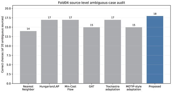
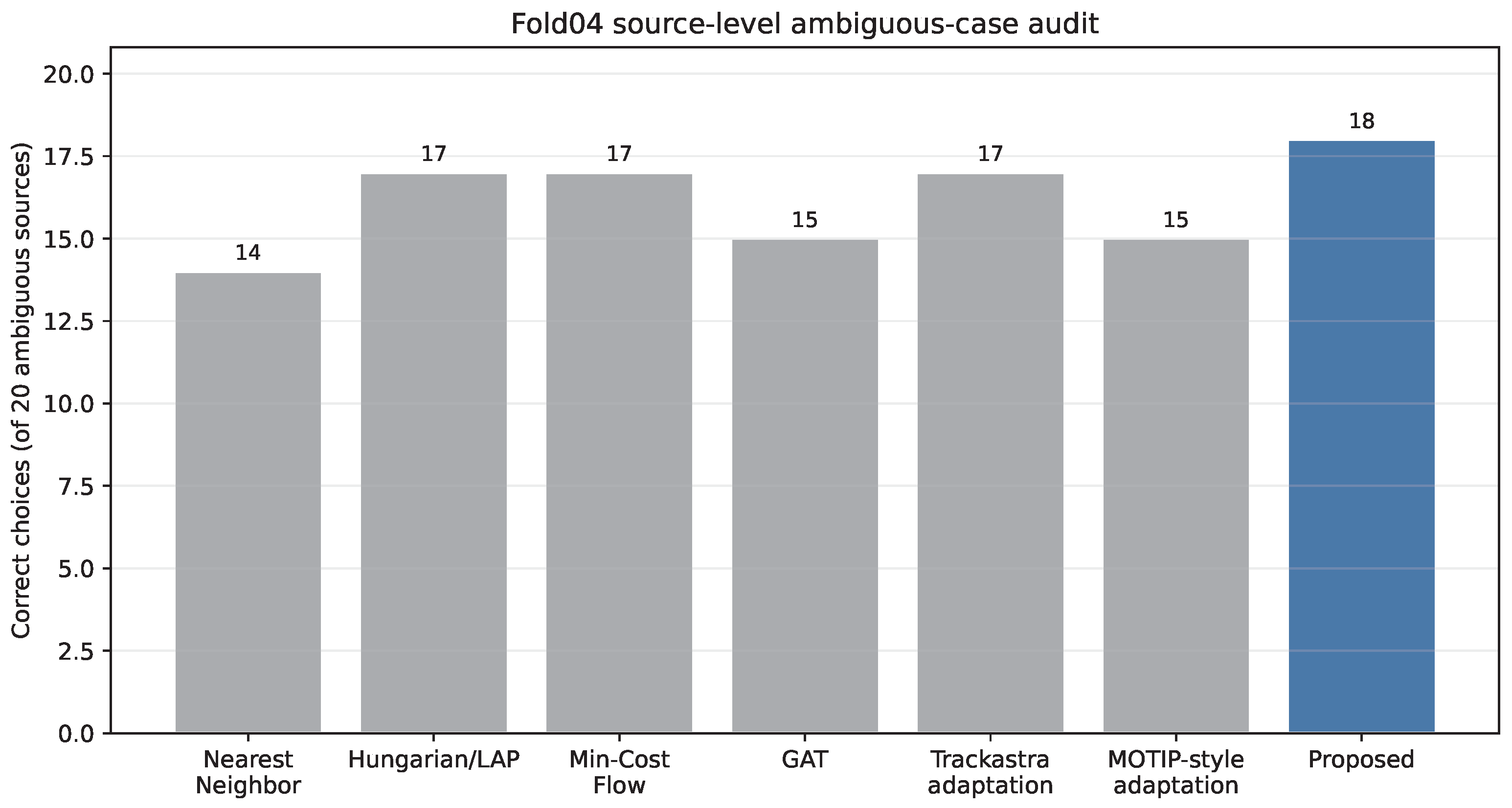
Figure 9 additionally reports the number of correct source choices on the manually reviewed ambiguous subset, providing a source-level view complementary to aggregate Link F1.

Figure 9. Fold04 source-level ambiguous-case audit. Correct selections are counted on the manually reviewed ambiguous-source subset.

5.8. Structural Proxies and Paired Statistics

The structural audit contained 132 GT gap opportunities across five folds, and all evaluated methods recovered zero gap bridges (Table 13). Root and leaf values are therefore terminal-behavior proxies rather than a separately validated stop classifier. The paired difference between the proposed method and Hungarian/LAP or min-cost flow was $+0.005405$ (bootstrap interval $[0,0.016216]$, $p=1.0$), which supports a non-regression and highest-observed-mean statement, not statistical superiority (Table 14).

Table 13. Claim-safe structural proxy summary.

Metric	Proposed Mean	Opportunities	Recovered
Path reachability F1	0.8999	–	–
Terminal root/leaf F1	proxy only	–	–
Gap bridge recovery	0.0000	132	0

Table 14. Selected paired comparisons.

Comparison	Mean Difference	Bootstrap 95% Interval	p
Proposed vs. Hungarian/LAP	+0.005405	[0, 0.016216]	1.000
Proposed vs. Min-cost flow	+0.005405	[0, 0.016216]	1.000
Proposed vs. Trackastra	+0.010526	[0, 0.031579]	1.000

6. Discussion

The results show that pore continuity recovery benefits from explicit cross-slice evidence and global feasibility constraints. CAPG-Link obtained the highest observed mean Link F1, $0.9846\pm 0.0344$. Against Hungarian/LAP and min-cost flow, it won one fold and tied four, with no fold-level loss. The small mean difference is therefore interpreted as a highest-observed-mean and non-regression result rather than evidence of statistical superiority. The difficult-case analysis further localizes the observed gain to a Fold-4 competing-candidate decision.

Under the fixed-node masking protocol, zeroing the designated continuity features reduced Link F1 in four of five folds, with reductions ranging from 0.1053 to 0.6000. Fold 1 showed no additional decrease because its reviewed gap edge was absent from the candidate graph. Among the grouped masks, displacement/distance produced the largest mean reduction, followed by intermediate-candidate context and slice-gap features. The joint and grouped results show that spatial displacement and cross-slice context are reflected in successor-selection performance, with different reduction magnitudes across the five folds.

Candidate coverage defines the recoverable scope of the association experiments: the frozen graph covered 95.31% of annotated nodes and 92.16% of annotated links, with 9 of 13 complete tracks represented. These measurements provide the deployment ceiling for extending the linker to full-volume detector outputs.

Continuity supervision is currently available for reviewed pore identities, while terminal behavior is represented through the reported proxy measures; broader validation will require denser annotations and additional materials, resolutions, and pore morphologies. Trackastra and MOTIP are evaluated as task adaptations.

7. Conclusions

CAPG-Link provides a structured way to turn slice-wise pore observations into reviewed cross-slice identities and local connectivity decisions that can support downstream pore persistence, track extent, and connectivity analysis. On the shared frozen candidate graphs, it achieved the highest observed mean Link F1 ($0.9846$) with no fold-level loss against the assignment baselines. The fixed-node masking experiment further showed that removing the designated continuity inputs reduced association performance in four of five folds, with displacement/distance features producing the largest isolated group effect. These results support the value of explicit cross-slice evidence for the association stage.

The reported association result is conditional on candidate availability. The measured node and directed-edge coverage, together with the incomplete full-track coverage, defines a deployment ceiling: a fully end-to-end system still requires detector-to-graph coverage over the complete XCT volume and denser, independently reviewed continuity annotations. Extending the benchmark across materials, resolutions, pore morphologies, and larger volumes will be needed to assess generalization beyond the present annotation-defined setting.

References

- Frazier, W.E. Metal additive manufacturing: A review. J. Mater. Eng. Perform. 2014, 23, 1917–1927. [Google Scholar] [CrossRef] [Scilit]
- DebRoy, T.; Wei, H.L.; Zuback, J.S.; Mukherjee, T.; Elmer, J.W.; Milewski, J.O.; Beese, A.M.; Wilson-Heid, A.; De, A.; Zhang, W. Additive manufacturing of metallic components—Process, structure and properties. Prog. Mater. Sci. 2018, 92, 112–224. [Google Scholar] [CrossRef] [Scilit]
- Leuders, S.; Thöne, M.; Riemer, A.; Niendorf, T.; Tröster, T.; Richard, H.A.; Maier, H.J. On the mechanical behaviour of titanium alloy TiAl6V4 manufactured by selective laser melting: Fatigue resistance and crack growth performance. Int. J. Fatigue 2013, 48, 300–307. [Google Scholar] [CrossRef] [Scilit]
- Yadollahi, A.; Shamsaei, N. Additive manufacturing of fatigue resistant materials: Challenges and opportunities. Int. J. Fatigue 2017, 98, 14–31. [Google Scholar] [CrossRef] [Scilit]
- Slotwinski, J.A.; Garboczi, E.J.; Stutzman, P.E. Porosity measurements and analysis for metal additive manufacturing process control. J. Res. Natl. Inst. Stand. Technol. 2014, 119, 494–528. [Google Scholar] [CrossRef] [Scilit] [PubMed]
- Thompson, A.; Maskery, I.; Leach, R.K. X-ray computed tomography for additive manufacturing: A review. Meas. Sci. Technol. 2016, 27, 072001. [Google Scholar] [CrossRef] [Scilit]
- du Plessis, A.; Yadroitsev, I.; Yadroitsava, I.; Le Roux, S.G. X-ray microcomputed tomography in additive manufacturing: A review of the current technology and applications. 3D Print. Addit. Manuf. 2018, 5, 227–239. [Google Scholar] [CrossRef] [Scilit]
- Withers, P.J. X-ray nanotomography. Mater. Today 2007, 10, 34–41. [Google Scholar] [CrossRef] [Scilit]
- Maire, E.; Withers, P.J. Quantitative X-ray tomography. Int. Mater. Rev. 2014, 59, 1–43. [Google Scholar] [CrossRef] [Scilit]
- Cnudde, V.; Boone, M.N. High-resolution X-ray computed tomography in geosciences: A review of the current technology and applications. Earth-Sci. Rev. 2013, 123, 1–17. [Google Scholar] [CrossRef] [Scilit]
- Bewley, A.; Ge, Z.; Ott, L.; Ramos, F.; Upcroft, B. Simple online and realtime tracking. In Proceedings of the IEEE International Conference on Image Processing (ICIP); IEEE: Piscataway, NJ, USA, 2016; pp. 3464–3468. [Google Scholar] [CrossRef] [Scilit]
- Wojke, N.; Bewley, A.; Paulus, D. Simple online and realtime tracking with a deep association metric. In Proceedings of the IEEE International Conference on Image Processing (ICIP); IEEE: Piscataway, NJ, USA, 2017; pp. 3645–3649. [Google Scholar] [CrossRef] [Scilit]
- Dendorfer, P.; Osep, A.; Milan, A.; Schindler, K.; Cremers, D.; Reid, I.; Roth, S.; Leal-Taixé, L. MOTChallenge: A benchmark for single-camera multiple target tracking. Int. J. Comput. Vis. 2021, 129, 845–881. [Google Scholar] [CrossRef] [Scilit]
- Luo, W.; Xing, J.; Milan, A.; Zhang, X.; Liu, W.; Kim, T.-K.; Yang, S. Multiple object tracking: A literature review. Artif. Intell. 2021, 293, 103448. [Google Scholar] [CrossRef] [Scilit]
- Ronneberger, O.; Fischer, P.; Brox, T. U-Net: Convolutional networks for biomedical image segmentation. In Medical Image Computing and Computer-Assisted Intervention—MICCAI 2015; Springer: Cham, Switzerland, 2015; pp. 234–241. [Google Scholar] [CrossRef] [Scilit]
- Ren, S.; He, K.; Girshick, R.; Sun, J. Faster R-CNN: Towards real-time object detection with region proposal networks. In Advances in Neural Information Processing Systems; NeurIPS: La Jolla, CA, USA, 2015; Volume 28, pp. 91–99. [Google Scholar]
- Redmon, J.; Divvala, S.; Girshick, R.; Farhadi, A. You only look once: Unified, real-time object detection. In Proceedings of the IEEE Conference on Computer Vision and Pattern Recognition (CVPR); IEEE: Piscataway, NJ, USA, 2016; pp. 779–788. [Google Scholar] [CrossRef] [Scilit]
- Lin, T.-Y.; Goyal, P.; Girshick, R.; He, K.; Dollár, P. Focal loss for dense object detection. In Proceedings of the IEEE International Conference on Computer Vision (ICCV); IEEE: Piscataway, NJ, USA, 2017; pp. 2980–2988. [Google Scholar] [CrossRef] [Scilit]
- Dai, J.; Li, T.; Xuan, Z.; Feng, Z. Automated defect analysis system for industrial computerized tomography images of solid rocket motor grains based on YOLO-V4 model. Electronics 2022, 11, 3215. [Google Scholar] [CrossRef] [Scilit]
- Wang, J.; Lin, B.; Li, G.; Zhou, Y.; Zhong, L.; Li, X.; Zhang, X. YOLO-Xray: A bubble defect detection algorithm for chip X-ray images based on improved YOLOv5. Electronics 2023, 12, 3060. [Google Scholar] [CrossRef] [Scilit]
- Kuhn, H.W. The Hungarian method for the assignment problem. Nav. Res. Logist. Q. 1955, 2, 83–97. [Google Scholar] [CrossRef] [Scilit]
- Jonker, R.; Volgenant, A. A shortest augmenting path algorithm for dense and sparse linear assignment problems. Computing 1987, 38, 325–340. [Google Scholar] [CrossRef] [Scilit]
- Zhang, L.; Li, Y.; Nevatia, R. Global data association for multi-object tracking using network flows. In Proceedings of the IEEE Conference on Computer Vision and Pattern Recognition (CVPR); IEEE: Piscataway, NJ, USA, 2008; pp. 1–8. [Google Scholar] [CrossRef] [Scilit]
- Kipf, T.N.; Welling, M. Semi-supervised classification with graph convolutional networks. In Proceedings of the International Conference on Learning Representations (ICLR); OpenReview: Vancouver, BC, Canada, 2018. [Google Scholar]
- Gilmer, J.; Schoenholz, S.S.; Riley, P.F.; Vinyals, O.; Dahl, G.E. Neural message passing for quantum chemistry. In Proceedings of the 34th International Conference on Machine Learning (ICML); PMLR: Sydney, Australia, 2017; Volume 70, pp. 1263–1272. [Google Scholar]
- Hamilton, W.; Ying, Z.; Leskovec, J. Inductive representation learning on large graphs. In Advances in Neural Information Processing Systems; NeurIPS: La Jolla, CA, USA, 2017; Volume 30. [Google Scholar]
- Veličković, P.; Cucurull, G.; Casanova, A.; Romero, A.; Liò, P.; Bengio, Y. Graph attention networks. In Proceedings of the International Conference on Learning Representations (ICLR); OpenReview: Vancouver, BC, Canada, 2018. [Google Scholar]
- Liu, Y.; Wen, T.; Wu, Z. Motion artifact detection based on regional–temporal graph attention network from head computed tomography images. Electronics 2024, 13, 724. [Google Scholar] [CrossRef] [Scilit]
- Sadeghian, A.; Alahi, A.; Savarese, S. Tracking the untrackable: Learning a deep association metric with a LSTM. In Proceedings of the IEEE International Conference on Computer Vision (ICCV); IEEE: Piscataway, NJ, USA, 2017. [Google Scholar]
- Gao, R.; Qi, J.; Wang, L. Multiple object tracking as ID prediction. In Proceedings of the IEEE/CVF Conference on Computer Vision and Pattern Recognition (CVPR); IEEE: Piscataway, NJ, USA, 2025. [Google Scholar]
- Sun, S.; Shi, C.; Wang, C.; Zhou, Q.; Sun, R.; Xiao, B.; Ding, Y.; Xi, G. Intra-frame graph structure and inter-frame bipartite graph matching with ReID-based occlusion resilience for point cloud multi-object tracking. Electronics 2024, 13, 2968. [Google Scholar] [CrossRef] [Scilit]
- Wei, Y.; Li, H.; Yu, B.; Lin, F. A hybrid manufacturing route to high-melting-point metallic lattice structures: Integrating material design with process innovation. J. Mater. Res. Technol. 2026, 41, 7547–7561. [Google Scholar] [CrossRef] [Scilit]
Disclaimer/Publisher’s Note: The statements, opinions and data contained in all publications are solely those of the individual author(s) and contributor(s) and not of MDPI and/or the editor(s). MDPI and/or the editor(s) disclaim responsibility for any injury to people or property resulting from any ideas, methods, instructions or products referred to in the content. |
© 2026 by the authors. Licensee MDPI, Basel, Switzerland. This article is an open access article distributed under the terms and conditions of the Creative Commons Attribution (CC BY) license.