


Abstract
Plant diseases pose a serious threat to agriculture, causing yield losses of 20 to 40 percent each year, resulting in more than USD 220 billion in annual economic losses and significantly affecting the global food supply. Traditional plant health monitoring practices involve visual inspection of plant tissue and can only detect the presence of disease once visual symptoms are already evident. This article presents AgriIDIA, a multispectral plant disease classification system based on 24-channel image stacks multispectral images derived from six optical filters (BlueIR, Hotmirror, K590, K665, K720, and K850) and six vegetation indices (NDVI, GNDVI, NDRE, EVI, REI, and SAVI). First, an exploratory data analysis is conducted on the diagnostic capability of the described 24-channel data representation, using 1266 image stacks labeled with six classes (diseased/healthy papaya, diseased/healthy potato, and diseased/healthy tomato). Next, using the results of the exploratory data analysis, the manuscript describes the training and cross-validation performance of AgriIDIA, with a macro-F1 score of 83.91 ± 3.42% and an accuracy of 84.00 ± 3.17% on the validation set. Finally, the performance of the trained model is evaluated on the reserved test set (N = 190), demonstrating an accuracy of 80.53%, a macro-F1 score of 0.7398, and a weighted ROC-AUC of 0.9383. The results of this study suggest that the 24-channel multispectral representation has significant diagnostic potential for distinguishing healthy and diseased plant tissue under the evaluated conditions.
1. Introduction
Plant diseases are among the leading and persistent threats to global agriculture and vegetable cropping systems. Based on their analysis, Strange and Scott [1] estimated that 10–16% of global food crop production is lost each year due to pathogens, with the burden being higher in tropical regions. Many of the funds used may also result in non-target organisms that are lost due to land degradation and biodiversity [2]. Research by Savary et al. [3] is based on a survey conducted with 494 experts from 67 nations that has shown that loss between the five most valuable crops reaches levels of about 17.2–30.0% of their potential annual production, equivalent to c.a. 300–600 million people going hungry yearly for lack of this nutritional source. It was also pointed out [4] that climate change, globalization of trade, and the erosion of biodiversity are creating a framework in which global plant disease pandemics occur. According to the Food and Agriculture Organization of the United Nations (FAO), plant diseases cause global economic losses exceeding USD 220 billion annually [5].
In Latin America, pests and diseases reduce the production of essential crops by 20 to 25 percent. This threatens the livelihoods of more than 60 million smallholder farmers [6]. In Peru, the situation is critical because of (i) an exceptional diversity of microclimates that leads to many pathogens; (ii) a lack of rural plant pathology infrastructure; and (iii) dependence on agrochemicals as the only control method, which causes health issues, pollution, and resistance. An automated early-detection system that looks at multispectral images could help change this cycle by allowing targeted and timely interventions with lower doses of agrochemicals.
The dominant paradigm of plant health monitoring via periodic visual inspection by specialized agronomists has three structural limitations that no incremental improvement can overcome without a technological paradigm shift:
A pre-symptomatic spectral window invisible to the human eye. Infected tissue changes its reflectance in the near-infrared (NIR) (700–1000 nm) and red-edge (680–730 nm) bands between 3 and 14 days before visible symptoms appear [7,8]. Indices such as NDRE and REI are physiologically sensitive indicators of presymptomatic changes.
Insufficient spatial/temporal coverage. Continuous monitoring through human inspection is economically unfeasible in most Latin American contexts.
Laboratory-to-field gap. RGB classifiers achieve >99% accuracy in the laboratory, but their accuracy drops by up to 30 points in real-world field conditions [9,10].
Multispectral imagery overcomes the three limitations of this study. The vegetation indices derived from the spectral bands mentioned above can serve as excellent biomarkers of physiological parameters, such as chlorophyll content, stomatal opening, and photosynthetic activity [7,8,11,12,13,14,15,16]. Together with EfficientNet [17], they enable non-invasive and automated diagnosis. Literature lacks information on the following aspects:
Gap 1 (pipeline): No previous work has mathematically formalized a stack of 24 spectral channels (18 filters + 6 indices) as input to a plant health CNN. Gap 2 (initialization): Adapting pre-trained RGB architectures to >3 channels lacks formal mathematical justification [18,19]. Gap 3 (evaluation): The prevailing practice of using single partitions without variance estimation [20,21] prevents an assessment of robustness.
The objective of this work is to develop and evaluate AgriIDIA, a multispectral plant disease classification system based on transfer learning applied to 24-channel multispectral stacks, featuring a complete mathematical formalization of the pipeline, a variance-preserving adaptation of EfficientNet-B0 from 3 to 24 channels, and rigorous evaluation through five-fold stratified cross-validation using an independent test set. The specific contributions are as follows:
Complete formalization of the 24-channel multispectral pipeline using 19 equations. A weighted-average initialization scheme with variance preservation for scaling EfficientNet-B0 from 3 to 24 channels. Statistically rigorous evaluation protocol using SFCV, a separate test set, and an F1-macro report with variance. Comprehensive exploration data analysis to validate spectral separability between classes.
Section 2 outlines the state of the art in five categories: phytosanitary spectral images, CNNs for plant disease classification, efficient CNN architectures and transfer learning, regularization and optimization, and evaluation metrics. In Section 3, we describe the materials and methods of the current workflow. We present the results of our experiments in Section 4 in terms of SFCV per fold, metrics per class on the test set, confusion matrices, and comparisons with the literature. Finally, we discuss the results in detail in the context of the state of the art in Section 5 and conclude the paper in Section 6 by reaffirming our contributions and suggesting directions for future research.
2. Related Works
2.1. Spectral Imaging for Early Plant Health Detection
It is difficult to overstate the strength of the scientific consensus on this point: that the most diagnostic and sensitive spectral bands for plant infection are found in the near-infrared (NIR, 700–1000 nm) and the red edge (RE, 680–730 nm). The most comprehensive study on this topic to date [7] systematically tested wheat, barley, and sugar beets for spectral responses to infection and found that while the spectra in the visible bands (400–700 nm) changed significantly only in the period immediately preceding the appearance of visible symptoms, the change in reflectance in the NIR and RE bands appeared 3 to 14 days earlier. The same conclusion, albeit using the example of Xylella fastidiosa in olive trees, was also supported by [22], whose research showed that spectral markers of infection became visible to the naked eye 12 months after the onset of infection. Taken together, this demonstrates that red-edge and near-infrared (NIR) wavelengths are the most sensitive to any plant infection, making them the most valuable for early detection. Mahlein et al. [8] took the topic a step further by developing specific spectral indices for the detection of foliar diseases, also in wheat. They found that simple vegetation indices, designed for the general assessment of plant health, were outperformed by measurements centered on the red edge (680–730 nm): specifically, for the detection of Cercospora beticola, the NDRE index produced a separation of 2.3 standard deviations (SD) from the healthy plant control during the pre-symptomatic period, compared with 0.4 SD for the conventional NDVI. This is perhaps the most direct evidence presented in the article regarding the usefulness of the NDRE and, specifically, of red-edge indices for detecting plant infections, which directly supports the application of AgriIDIA.
As regards the choice between derived indices and unprocessed bands, Sankaran et al. [23] analyzed the most frequently cited review study (112 publications) in this field of research and noted that multispectral imagery and associated reflectance indices can successfully detect water stress, nutrient deficiency, and various fungal and bacterial diseases with a resolution ranging from 5 to 21 days, depending on the specific pathogen. The main conclusion of this study was that the key limitation to the adoption of these methods is not their accuracy, but rather the lack of standardized and validated protocols for transforming raw spectral data into a format suitable for training classifiers. This conclusion became one of the driving forces behind our research, leading to the mathematical formulation of AgriIDIA. Specifically, Lowe et al. [24] experimentally evaluated the contribution of individual spectral indices to the detection of phylloxera and demonstrated that the combined use of all indices outperformed the performance of each index by a significant margin at all observation time points following inoculation (3, 7, 10, and 14 days). Furthermore, the most notable performance improvement was observed at the early time points (3–7 days), suggesting that the information content of the additional indices is not redundant but rather complementary in the early stages of disease development. This observation directly supports our decision to use six spectral indices in AgriIDIA rather than a smaller subset.
Methodologically, Behmann et al. [25] used a quantitative meta-analysis covering 47 primary studies to establish three basic rules: (i) mixing red-edge spectral indices with supervised classifiers beats purely unsupervised spectral methods regarding F1-score in every context checked; (ii) models built from lab data show an average accuracy loss of 18.3% when tested on field data versus just 6.7% for those made from field data; and (iii) stratified cross-validation is the sole protocol giving statistically unbiased performance estimates on new data since single partitions inflate real accuracy by 7–12% on average. These three findings create direct literature bases for AgriIDIA’s methodological design, using SFCV, a held-out test set, and reporting statistical variance as standard steps to guarantee result reproducibility and comparability.
2.2. Deep Learning for Classifying Plant Diseases
The arrival of convolutional neural networks (CNNs) and transfer learning signaled a shift in automatic plant disease detection, yet major constraints soon emerged concerning model portability from lab settings to actual field situations. Mohanty et al. [9] performed the initial research with the highest citation counts here, training GoogLeNet and AlexNet on 54,306 RGB images from the PlantVillage archive, covering 26 illnesses across 14 crop varieties shot against consistent backdrops under steady light and reaching validation accuracy of 99.35%. However, the writers openly admitted in their final remarks that models were developed and tested on pictures taken under very similar lab settings, that moving to real-world settings remained unverified, and that the main goal now was building sets recorded under environmentally typical settings. This warning was measured numerically by [10], who made PlantDoc, the earliest plant illness set recorded outside fields lacking control over backdrop, illumination, or viewpoint, containing 2598 RGB pictures of 17 sickness groups across 13 plants. While testing four pre-trained models on this collection, they noted accuracy losses varying from 18.7 to 31.4 percentage points versus figures stated on PlantVillage for identical models.
About spectral information beyond the visible spectrum, the most direct precursor to AgriIDIA is the work of Picon et al. [21], who developed a system based on a convolutional neural network (CNN) to classify tomato leaf diseases using portable four-band (RGB + NIR) multispectral cameras controlled via mobile devices under semi-controlled conditions. They reported over 90% accuracy for multispectral models compared to 83% for RGB equivalents on the same dataset, with a 7-point improvement attributed exclusively to NIR information. The authors concluded that NIR spectral fusion consistently outperforms visible-space approaches for early detection of foliar infections, providing the empirical justification for extending from 4 to 24 spectral channels in AgriIDIA. When comparing the performance of multispectral models against equivalent RGB models on the same dataset, they reported accuracy exceeding 90% for the former, compared to 83% for the latter, with an average improvement of 7 percentage points attributed exclusively to NIR information. The authors concluded that NIR spectral fusion consistently outperforms the visible spectrum for the early detection of foliar infections, thus providing the most direct empirical evidence justifying the expansion from 4 to 24 spectral channels in AgriIDIA. From a methodological perspective, Kamilaris and Prenafeta-Boldú [26] conducted the most extensive bibliometric review on deep learning in agriculture (40 studies selected using PRISMA criteria), concluding that most studies in the field suffer from methodologically weak evaluations such as single partitions without variance estimation, that laboratory datasets do not predict real-world field performance, and that the absence of statistical robustness metrics such as ROC-AUC makes it impossible to statistically compare systems proposed in different studies. The review identifies SFCV, ROC-AUC, and retained test sets as the three practices necessary to overcome the current state of the art, all of which are implemented in AgriIDIA. Finally, Barbedo [27] examined the factors that limit the practical applicability of deep learning systems for plant disease detection, identifying class imbalance, intra-class variability, and background noise as the three factors with the greatest negative impact on generalization.
2.3. Efficient CNN Architectures and Transfer Learning for Agricultural Images
The constant quest for a balance between representational capacity and computational efficiency characterizes the evolution of convolutional neural network architectures. This is a fundamental aspect for precision agriculture, a field in which hardware limitations are often encountered. Simonyan and Zisserman [28], through their work on VGGNet, revealed that a constant depth achieved with 3 × 3 filters stand out as the most important determining factor for classification accuracy at larger scales. VGG-16 and VGG-19, with 138 and 144 million parameters, respectively, were the most widely used models for transfer learning in plant disease detection between 2016 and 2020 [20], establishing the viability of the ImageNet fine-tuning paradigm for the plant health domain. However, their high computational cost prompted the search for more efficient architectures, which culminated in ResNet and, subsequently, in EfficientNet. He et al. [28] introduced ResNet with the aim of addressing the problem of performance degradation when increasing the depth of networks beyond 20 layers. Residual skip connections, which learn residuals F(x) = H(x) − x instead of the full function H(x), enabled the stable training of networks with up to 152 layers, setting new accuracy records on ImageNet, COCO, and Pascal VOC. With over 250,000 citations on Google Scholar, ResNet establishes the residual learning paradigm that EfficientNet inherits through its MBConv (Mobile Inverted Bottleneck Convolution) blocks.
Tan and Le [17] introduced EfficientNet with a novel approach: systematic composite scaling of depth, width, and resolution using a single composite scaling coefficient φ, rather than scaling each dimension independently and arbitrarily as in previous work. Through neural architecture search (NAS) to find the optimal scaling coefficients under the constraint α ⋅ β2 ⋅ γ2 ≈ 2, they derived the EfficientNet family from B0 to B7. EfficientNet-B0, with only 5.3 million parameters, outperformed ResNet-50 (26 M) and VGG-16 (138 M) in top 1 accuracy on ImageNet with approximately 8- and 26-times fewer parameters, respectively. The key conclusion of this work is that composite scaling is the most efficient network design strategy available and that B0 provides the best performance-to-efficiency ratio for applications with memory and computational constraints, which is a decisive factor in the selection of this architecture at AgriIDIA, given the computational context of Peruvian agriculture.
Regarding the stability of deep network training, He et al. [18] proposed He initialization (or Kaiming initialization) with the goal of stabilizing the training of networks with rectified activations. Through a formal analysis of the forward propagation of activation variance and the backward propagation of gradients through convolutional layers with ReLU, they demonstrated that the correct scaling factor for the initial weights of a layer with Cin input channels and a k × k is under ReLU and under linear activations. Failure to satisfy this condition in the first input layer can propagate to deeper layers, causing gradient explosion or vanishing gradients from the start of training. Previously, Glorot and Bengio [19] had addressed the difficulty of training deep networks with sigmoid and tanh activations, demonstrating that the variance of activations and gradients decays exponentially with depth when weights are initialized without considering the number of connections. Glorot’s criterion (or Xavier initialization) preserves variance under the assumption of symmetry in the activations Var[W] = 2/(nin + nout). Although the criterion was later extended [18] to asymmetric activations (ReLU), Glorot and Bengio established the fundamental principle that initialization must be a function of the number of connections. The factor 3/Cin in Equation (11) of this paper is a direct instance of this principle, applied specifically to the adaptation of EfficientNet-B0 from 3 to 24 input channels.
Pan and Yang [29] published the most-cited review on transfer learning, formalizing the conditions under which knowledge from a source domain transfers beneficially to a target domain. Their findings on the importance of feature distribution similarity between domains justify using ImageNet-pretrained weights in a multispectral context: while the 24 input channels differ spectrally from ImageNet’s RGB, high-level visual features such as edges, textures, and shapes remain transferable. The two-stage fine-tuning protocol detailed in Section 5.2 further ensures proper adaptation to the target domain. This theoretical foundation, combined with EfficientNet-B0’s computational efficiency and the stability guaranteed by He and Glorot initialization schemes, constitutes the architectural core of AgriIDIA.
2.4. Standardization, Optimization, and Metrics
The stability of AgriIDIA is underpinned by appropriate regularization, optimization, and evaluation techniques. Batch normalization [30] and label smoothing [31] help to stabilize training and reduce overfitting, particularly in small and imbalanced datasets [32,33]. Hutter [34] is used for optimization, whilst performance is evaluated using macro-F1 and AUC, metrics recommended for multi-class classification and imbalanced problems [35,36]. Cross-validation also allows the variability of the results to be estimated.
2.5. Summary of Research Gaps
The above review makes it possible to precisely identify three gaps that AgriIDIA addresses simultaneously and in a complementary manner:
Gap 1 (pipeline): No previous work has mathematically constructed and formalized a unified stack of 24 spectral channels, 18 optical filters plus 6 vegetation indices as direct input to a CNN for phytosanitary classification. Existing studies use between 2 and 4 bands without integrating the six indices, whose diagnostic complementarity has been documented [7,8,24]. Gap 2 (initialization): The adaptation of pre-trained RGB architectures to multispectral inputs with more than three channels requires careful consideration of weight scaling when the number of input channels is increased. In this study, we formulate a variance-preserving initialization scheme for adapting EfficientNet-B0 from 3 to 24 input channels, based on the initialization criterion in [18]. Gap 3 (evaluation): The most influential studies in this field [9,20,21] report results based on single partitions without variance estimation. SFCV with an independent test partition and ROC-AUC is the standard required to address this methodological shortcoming, as identified in [25,26].
3. Materials and Methods
3.1. Pipeline Overview
AgriIDIA implements a four-stage sequential pipeline whose statistical integrity is ensured by the strict separation of partitions at all stages of processing.
Stage 1: Multispectral acquisition and synthesis. Images from the primary source (Google Storage Dataset 3) are acquired using six optical filters that provide the 18 base reflectance channels (3 RGB channels per filter × 6 filters). Images from the secondary RGB sources (PlantVillage, PlantDoc) are transformed into pseudo-multispectral stacks using the spectral synthesis described in Section 3.2.1.
Stage 2: Exploratory data analysis (EDA). Statistical characterization of the 24 channels, analysis of class distribution, statistical separability, and correlations among spectral indices.
Step 3: Construction of the 24-channel stack. Radiometric correction using percentile stretching (Section 3.2.2), calculation of six vegetation indices (Section 4.2), concatenation of 18 reflectance channels with 6 indices, and statistical normalization by channel (Section 4.3).
Step 4: Partitioning and cross-validation. The test partition (N = 190, 15%) is extracted before any further processing using stratified sampling (seed = 42). Five stratified folds are constructed from the remaining N = 1076 stacked samples. For each fold, the two training phases described in Section 5.2 are run, and the checkpoint with the highest validation macro-F1 score is retained.
Step 5: Training and evaluation. The fold with the highest validation F1-macro is evaluated once on the sealed test set, calculating all metrics listed in Section 3.11.
3.2. Exploratory Data Analysis (EDA)
3.2.1. Composition of the Dataset
The AgriIDIA dataset was constructed from three main sources, combining real multispectral imagery with RGB images from public repositories to enhance the representativeness of the classes. The primary source is Google Storage Dataset 3, which provides 442 real-world multispectral stacks captured using six optical filters (BlueIR, Hotmirror, K590, K665, K720, and K850) on papaya, potato, and tomato specimens under semi-controlled field conditions. To supplement the classes with the least amount of real-world data, particularly in the potato and tomato disease categories, RGB images from the PlantVillage [9] and PlantDoc [10] repositories were incorporated, totaling 824 pseudo-multispectral stacks generated via spectral synthesis (Equations (3) and (4)). Before final integration, raw images endured a thorough quality filtering stage utilizing radiometric standards (P2 and P98 percentiles, dynamic range, and minimal vegetation cover), subsequently removing 1.4 percent of the initial images (38 images). After that, a fixed-seed stratified sampling method (42) was utilized to guarantee the test partition (15 percent of the total, N = 190) mirrored the classes’ natural spread and was totally kept apart from any training stage or hyperparameter selection, this helping avoids information bleeding. With the dataset left (Train + Val, N = 1076), a five-fold stratified cross-validation technique was put into practice, keeping the initial class proportions within each fold. The final makeup of the dataset post clustering, quality filtering, and stratified partitioning is laid out in Table 1.
Table 1.
Complete composition of the AgriIDIA dataset.
Of the 1266 image stacks included in the dataset, 442 (34.9%) correspond to physical multispectral acquisitions, whereas 824 (65.1%) are pseudo-multispectral stacks generated from RGB images. Therefore, the dataset is predominantly composed of synthesized multispectral data. This composition should be considered when interpreting the generalization of the model to physical multispectral imagery.
The considerable amount of synthetic data (65.1 per cent of the total) highlights just how scarce real multispectral images of Andean crops are. The dataset comprises six distinct categories, which have been artificially balanced by incorporating synthetic examples. Within this dataset, the ‘diseased tomato’ category stands out as the largest, with 636 examples (of which 74 are real and 562 are synthetic); this is followed by ‘diseased potato’, with 311 (105 real and 206 synthetic); ‘healthy tomato’, with 130 (74 real and 56 synthetic); ‘healthy potato’, with 80 (all real); ‘healthy papaya’, with 60 (all real); and ‘diseased papaya’, which brings up the rear with 49 (all real). This specific distribution clearly indicates the limited availability of real multispectral images for the ‘healthy papaya’ and ‘healthy potato’ groups, which have therefore been supplemented with synthetic images from PlantVillage and PlantDoc for the potato and tomato categories, respectively, whilst the papaya categories cannot rely on synthetic equivalents due to the lack of a comparable public database.
3.2.2. Analysis of the 24 Spectral Channels
Table 2 presents descriptive statistics for the 24 channels calculated from a representative sample (30 images per class). The spectral indices exhibit wide dynamic ranges (deviations > 0.34), indicating high variability among phytosanitary conditions. The GNDVI has the highest standard deviation (0.5897), indicating greater variability in this index across the analyzed samples.
Table 2.
Descriptive statistics for the 24 channels of the multispectral stack.
3.2.3. Statistical Separability Between Classes
The non-parametric Mann–Whitney U test was used to compare the spectral indices between healthy and diseased plants within each species (Table 3). In potatoes, GNDVI and NDRE showed significant differences (p < 0.01); in papaya, EVI was significant (p < 0.05), whilst in tomatoes, GNDVI was found to be significant (p < 0.05). These results indicate that the ability of the indices to differentiate between healthy and diseased plants depends on the species analyzed.
Table 3.
Mann–Whitney U Test for spectral indices (p-values).
To supplement the statistical separability analysis presented in Table 3, the entire spread of the six spectral indices is visualized via box plots delineated by class in Figure 1. This visual format lets us gauge the extent of overlap between healthy and diseased conditions for every species; furthermore, we can see which indices show clearer distributions and thus higher discriminating power.
Figure 1.
Distribution of spectral indices by crop and health status. Box colors distinguish the six categories shown on the x-axis; the horizontal dashed line indicates an index value of zero.
Figure 1 shows the distribution of the NDVI across the six categories for papaya, potato, and tomato, under healthy and diseased conditions. The box plots reveal a marked overlap between the classes, with medians close to 0.05–0.15 and interquartile ranges that include both negative and positive values. This behavior indicates that NDVI alone has limited ability to distinguish between healthy and diseased plants, particularly in papaya and tomato. In potato, a slight increase in values is observed in healthy plants, although the distributions remain overlapping. These results are consistent with those reported in [7,8], where the NDVI is considered a general indicator of plant vigor, with lower sensitivity to early-stage abnormalities. In contrast, indices such as the NDRE, REI, and GNDVI demonstrate greater discriminatory power, as shown by the separability analysis in Table 3.
3.2.4. Correlation Analysis of Spectral Indices
Figure 2 shows the Spearman’s correlation matrix between the six spectral indices, together with a scatter plot of NDVI versus REI, categorized by class. A very high correlation is observed between NDVI and SAVI (0.934), whilst EVI also shows strong correlations with both indices (0.782 and 0.826), indicating a degree of redundancy amongst these variables. Meanwhile, the NDRE shows moderate correlations, ranging from 0.53 to 0.59, with most of the indices. In contrast, the REI shows virtually no correlation with GNDVI (−0.084) and NDRE (0.044), and a moderate correlation with EVI (0.45), suggesting that it provides different spectral information. This characteristic is also evident in the NDVI–REI plot, where the values are widely dispersed, and there is no clear separation between classes. Overall, the results support the inclusion of all six indices in the 24-channel stack, as although some provide similar information, others offer complementary signals that may help to improve the early identification of diseases [7,8,24].
Figure 2.
Correlation analysis of spectral indices in the AgriIDIA dataset. (a) Spearman correlation matrix for the six spectral indices. (b) Scatter plot of NDVI versus REI, with points colored by crop and health status. Dashed lines indicate zero on each axis.
The correlation analysis presented in Figure 2a and Table 4 shows clear differences in the relationship between the six spectral indices. The strongest association is found between NDVI and SAVI (0.934), followed by the correlations between EVI and NDVI (0.782) and SAVI (0.826), which indicates that these three indices contain partially similar information. In contrast, REI shows very weak relationships with GNDVI (−0.084) and NDRE (0.044), suggesting that it provides distinct spectral information linked to changes in plant tissue structure. This difference is also evident in the NDVI–REI scatter plot shown in Figure 2b, where the values are widely distributed and do not form clearly distinct clusters according to class. Taken together, the simultaneous presence of highly correlated indices, such as NDVI–SAVI–EVI, and others with more independent behavior, such as REI–GNDVI and REI–NDRE, supports the use of all six indices, as their combination allows for the retention of complementary information useful for the early identification of signs of infection, in line with the findings of Mahlein et al. [8] and Lowe et al. [24].
Table 4.
Spearman’s correlation matrix between spectral indices.
3.2.5. Displaying Spectral Indices
Figure 3 compares RGB images (BlueIR and K720) with six spectral indices for the same species in healthy and diseased states. Whilst the RGB images show barely visible differences, the spectral maps reveal more distinct changes. NDVI and SAVI show higher values in healthy plants, whilst REI and NDRE show variations related to the physiological state and structure of plant tissue. These results are consistent with Table 3, where NDRE and GNDVI demonstrated greater discriminatory power, supporting the use of multispectral data for the early detection of diseases [7,8].
Figure 3.
Comparative visualization of spectral indices: healthy plant vs. diseased plant.
3.3. Data Source
3.3.1. Primary Multispectral Source: Google Storage Dataset 3
The primary source is the collection known as Google Storage Dataset 3, which comprises 2652 JPEG images of foliage from three crops (papaya, potato, and tomato) in healthy and diseased states, captured using six interchangeable optical filters mounted on an APS-C digital camera under diffuse natural light in semi-controlled field conditions. The spectral regions, physiological relevance, and assigned channels of the six optical filters are summarized in Table 5.
Table 5.
Specifications for the six optical filters.
3.3.2. Complementary RGB Lights
To expand the disease classes for tomatoes and potatoes, two secondary sources of RGB images were incorporated:
PlantVillage [9] is the reference dataset for this field, containing 54,306 RGB images of 26 diseases in 14 crop species captured against uniform backgrounds under laboratory conditions. For AgriIDIA, the relevant classes were selected: 7958 images for tomato (early blight, late blight, leaf mold, septoria leaf spot, mosaic virus, bacterial spot, and healthy) and 2152 for potato (early blight, late blight, and healthy). The selection was made by excluding images of poor visual quality (blurry, overexposed, or containing artifacts) using the criteria outlined in Section 3.5.4.
PlantDoc [10] provides 2598 RGB images across 17 classes, captured under real-field conditions without controlled backgrounds or lighting. Between 101 and 180 images were selected per class relevant to potatoes and tomatoes. The inclusion of PlantDoc is intended to increase the ecological variability of the training data and reduce the laboratory-field gap for the synthetic classes.
No supplementary data sources were included for the papaya classes, as there is no equivalent public repository of RGB images of papaya with annotations of diseases relevant to the Andean context.
3.4. Technical Implementation Specifications
Framework: PyTorch 2.14-0+cuda, timm v0.9.130 for EfficientNet-B0 with ImageNet-1k weights, NumPy 1.24+, scikit-learn 1.3+.
Storage: Stacked float32 TIFF files (24, 224, 224) loaded using torchvision. transforms and DataLoader (num_workers = 4, pin_memory = True).
Imbalance Management: WeightedRandomSampler in the training DataLoader, supplementing class weights from the loss function [37].
Hardware: Intel Core i7 CPU, 16 GB RAM. Time per fold: 45–90 min, depending on the early-stop point.
Reproducibility: seed 42 in random, np.random, torch.manual_seed, and torch.cuda.manual_seed_all.
3.5. Mathematical Framework
3.5.1. Spectral Stacking Construction
The six filter images were not subjected to pixel-level co-registration; therefore, residual inter-filter spatial shifts of approximately 1–3 pixels may be present in the resulting multispectral stacks.
3.5.2. Notation and Band Extraction
The notation = {f1, f2, f3, f4, f5, f6} be the ordered set of six optical filters (BlueIR, Hotmirror, K590, K665, K720, and K850, respectively). For a plant specimen of class c ∈ {1, …, 6}, let I(fi) be the RGB image captured under filter fi with i ∈ {1, …, 6}, defined over the spatial domain (Equation (1)):
I(fi):Ω → [0,1]3, Ω = {(x,y)∣1 ≤ x ≤ H, 1 ≤ y ≤ W}
With H = W = 224 pixels after resizing using bilinear interpolation. The three channels of each filtered image are denoted by . The raw multispectral volume results from the ordered concatenation of the 18 frames along the channel axis:
Sraw = [R(f1), G(f1), B(f1), R(f2), G(f2), B(f2), …, R(f6), G(f6), B(f6)]⊤ ∈ [0,1]18×224×224
Channels 3(i − 1), 3(i − 1) + 1 y 3(i − 1) + 2 correspond to the R, G, and B planes of filter fi, respectively. Each filter modulates a different region of the reflectance spectrum; therefore, the 18 planes of the volume are spectrally non-redundant even though they share the same spatial resolution.
3.5.3. Spectral Synthesis for RGB Sources
The PlantVillage and PlantDoc images were not captured using the primary array’s physical filters; they are standard RGB images with bands centered at ~450 nm (B), ~550 nm (G), and ~650 nm (R). To construct pseudo-multispectral stacks from these images, synthetic spectral bands are derived using the correlations between visible and infrared reflectance documented in the quantitative remote sensing literature [38,39]:
NIRsint = clip(0.65 ⋅ R + 0.25 ⋅ G + 0.10 ⋅ (1 − B), 0,1)
REsint = clip(0.50 ⋅ R + 0.50 ⋅ NIRsint, 0,1)
The coefficient 0.65 applied to R in Equation (3) captures the inverse relationship between red reflectance and chlorophyll content established by [33]; the coefficient 0.25 applied to G incorporates the green reflectance peak of healthy tissue documented by Gitelson et al. [12]; the term 0.10(1 − B) compensates for the blue absorption of leaf pigments [11]. Equation (4) approximates the spectral inflection point at the red edge documented by [13]. Based on NIRsint y REsint, the six synthetic filter planes are constructed by linear combination to approximate the transmittance response of each physical filter.
3.5.4. Radiometric Correction and Quality Filtering
Images captured under variable natural light conditions exhibit differences in illumination between filters that must be corrected before calculating indices. Normalization by stretching is the standard method for this purpose in field imaging:
where Pk denotes the k-ésimo percentile of all values of channel c across the image. Using the P2 and P98 percentiles instead of the minimum and maximum makes the correction robust against extreme pixels caused by specular reflection or deep shadows. An image is rejected from the dataset if
Channel with μc < 0.02 or μc > 0.98 (dark or saturated image under a given filter);
Channel with (nearly uniform image, possibly blocked);
Pixel fraction with an “NDVI” value less than 0.10 or greater than 0.40 (insufficient vegetation cover for diagnosis).
Applying these criteria eliminated 38 images from the original total of 2690 available physical images (1.4%), resulting in the 442 physical stacks reported in Table 1.
3.6. Analytical Derivation of Vegetation Indices
The six vegetation indices (Equations (6)–(11)) are calculated using the corrected volume Scorr. Sea ε = 10−10 be the regularization constant to avoid division by zero. Proxy band assignments were made based on the spectral proximity between the transmittance response of each physical filter and the central band required by each index:
The complete 24-channel stacking is the result of concatenating the volume-corrected data with the six indices:
X = [Scorr; NDVI; GNDVI; NDRE; EVI; REI; SAVI] ∈ ℝ24×224×224
Channels 0–17 correspond to the 18 spectral bands, and channels 18–23 correspond to the six indices. All index values are normalized to the range [−1, 1]. Table 6 presents the physiological basis and canonical references for each index.
Table 6.
Physiological basis, canonical reference, and diagnostic function of each vegetation index in the AgriIDIA stack.
3.7. Statistical Normalization by Channel
The heterogeneity in the dynamic range across the 24 bands (reflectance in [0, 1] for channels 0–17 and indices in [−1, 1] for channels 18–23) requires normalization before the data is fed into the network. Each channel c ∈ {0, …, 23} is normalized using the statistics from the training partition of fold k:
The statistics and are calculated over the pixels of all training stacks in fold k for channel c and are applied identically to the validation and test partitions of the same fold, thereby preventing information leakage between partitions. Table 7 reports the mean values of μc y σc for the six metrics in Fold 4.
Table 7.
Normalization statistics for the six indices in Fold 4 training.
3.8. Model Architecture and Weight Initialization
3.8.1. EfficientNet-B0 as the Base Architecture
EfficientNet-B0 [17] applies composite scaling of depth d, width w, and resolution r using the composite coefficient φ:
d = αφ, w = βφ, r = γφ, sujeto a α ⋅ β2 ⋅ γ2≈2
For B0, φ = 1 with (α, β, γ) = (1.2, 1.1, 1.15), resulting in 5.3 M parameters with an input resolution of 224 × 224 px. The architecture consists of an input layer (Stem), followed by seven stages of MBConv blocks with residual connections and SiLU activation:
The SiLU activation function is smooth, non-monotonic, and has a non-zero gradient for negative values, properties that empirically improve the training of deep networks compared to ReLU in fine-grained classification tasks [17]. The 1280-dimensional feature vector extracted by the final GAP layer of the backbone serves as the input to the classification head.
3.8.2. Down Sampling from 3 to 24 Channels: Initialization Scheme with Variance Preservation
The original first convolutional layer has weights Worig ∈ ℝ32×3×3×3 (32 output filters, 3 input channels, 3 × 3 kernel). To adapt it to Cin = 24 input channels while preserving the pre-trained knowledge,
Step 1. Calculate the average of Worig across the three RGB channels:
Step 2. The new tensor Wnew ∈ ℝ32×24×3×3 is initialized:
Formal derivation of the scaling factor. Assuming normalized inputs Xnorm with mean zero and variance per channel, and statistically independent weights Wnew, the variance of the pre-activation of the first layer is
Since (ignoring replication, which by design does not affect the variance):
Substituting into Equation (18):
For the original case, Cin = 3, . For Cin = 24, . The variance is reduced by a factor of 9/72 = 0.125 compared to the original case, keeping it within the functional range of the backbone. Without the factor 3/Cin, direct replication of Wmean would increase Var[z] by a factor of Cin/3 = 8, producing pre-activations with a variance 8× that expected and a potential activation explosion incompatible with the convergence of the pre-trained backbone according to [18].
3.8.3. Top of the Standings
The head replaces EfficientNet-B0’s original single linear layer with a deep module:
The SiLU activation (Equation (14)) in the hidden layer is consistent with the MBConv blocks in the backbone [17]. The BN layers follow the recommendation in [30]. The dropout rates and other training hyperparameters were fixed before the cross-validation procedure and were kept unchanged across all folds. Fold 4 was selected solely because it achieved the highest validation macro-F1 score before the final evaluation on the sealed test set.
3.9. Loss Function with Smooth Labels and Class Weights
To mitigate class imbalance (maximum ratio of 636:49), weighted cross-entropy loss with label smoothing is used:
where yc ∈ {0,1} is the one-hot label, pc is the SoftMax prediction, and wc is the class weight:
Table 8 reports the wc weights calculated on the training partition of Fold 4:
Table 8.
wc class weights for Fold 4. Higher weights compensate for classes with lower support.
3.10. Geometric Scaling with Spectral Coherence
One of six geometric transformations, selected uniformly at random, is applied identically to all 24 channels in the stack to preserve the spectral relationship between bands:
Ak ∈ {id, flip-H, flip-V, rot90°, rot180°, rot270°}, k∼Uniform{0, …, 5}
Adjustments to intensity (brightness, contrast, and saturation) and color transformations are explicitly excluded because they would alter the values of the individual spectral channels and, consequently, the vegetation indices. Spectral consistency, meaning that the same point on the leaf has the same value across all 24 channels regardless of geometric transformation, is a constraint that only geometric transformations satisfy. The goal of up sampling is to increase the number of samples for each class to 800 per training fold.
3.11. Evaluation Metrics
Let TPc, FPc, and FNc be the true positives, false positives, and false negatives of class c on the retained test set:
F1-macro is the primary metric for treating all classes equally regardless of the feature set [35]. The weighted ROC-AUC in OvR configuration is the threshold-independent discrimination metric [36]. Training and validation metrics are calculated at the end of each epoch; evaluation on the test set is performed once using the checkpoint from the best fold.
3.12. Experimental Configurations
3.12.1. Protocol for Five-Fold Stratified Cross-Validation
The Train + Val dataset (N = 1076) is divided into five stratified folds F1, …, F5 while preserving the class distribution. For fold k, the model is trained on samples and validated on Fk ≈ 215 samples. Table 9 details the class distribution across the five validation folds:
Table 9.
Class distribution across the five validation partitions of the SFCV.
3.12.2. Two-Phase Training
Phase 1: Head alignment (5 epochs). Frozen backbone (requires_grad = False for all parameters except the head). Optimizer: AdamW, lr1 = 10−3, λ = 10−4, β1 = 0.9, β2 = 0.999. Planner: cosine annealing with warm restarts (SGDR [40]), T0 = 10, Tmult = 2, ηmin = 10−6.
Phase 2: Complete fine-tuning (up to 40 epochs). All parameters are unfrozen. AdamW reset to lr2 = 10−4 with the same regularization and planner parameters. Early stopping with patience p = 8 epochs, monitoring . The checkpoint from the epoch with the highest in Phase 2 is retained for the final evaluation.
4. Results
4.1. Results of Stratified Cross-Validation
Table 10 presents the complete results of the SFCV. The mean accuracy was 0.8400 ± 0.0317, while the mean macro-F1 score was 0.8391 ± 0.0342. These results indicate relatively consistent performance across the five validation folds, although some variation was observed depending on the composition of each partition.
Table 10.
Results of the stratified five-fold cross-validation.
In phase 1 of cycle 4, the loss fell from approximately 1.95 in the first epoch to 1.20 in the fifth, showing a gradual decline without any noticeable fluctuations. This behavior supports the stability of the initialization scheme described in Section 3.8.2. During phase 2, the best result was obtained in epoch 20, with a validation macro-F1 of 0.8792, and training continued until epoch 28, when early stopping was applied.
Figure 4 shows the accuracy obtained across the five folds of the stratified cross-validation. The results ranged from 0.787 in the first fold to 0.880 in the fourth, with a mean of 0.8400 and a standard deviation of ±0.0317, equivalent to a coefficient of variation of approximately 4.2 per cent. Although some variation is observed between the folds, the values remain relatively stable. Fold 4 recorded the best result (0.880) and was selected for the final evaluation on the retained test set, whilst Fold 1 had the lowest value (0.787), demonstrating that performance may vary depending on the composition of the data used for training. Generally speaking, the similarity of the metrics across the different folds supports the stability of the initialization procedure used and suggests that the performance obtained is not determined by a single partition of the dataset [25].
Figure 4.
Accuracy per fold in cross-validation.
F1-macro mean = 0.8391 ± 0.0342. The coefficient of variation across folds (CV = 0.0342/0.8391 ≈ 4.1%) indicates moderate variability, consistent with [25] for datasets of comparable scale (N ≈ 1000–2000).
4.2. Detailed Metrics for Fold 4 Are Currently Being Validated
Table 11 presents the classification metrics obtained on Fold 4 of the validation set, which was selected for the final evaluation as it achieved the highest macro-F1 score (0.8792). The most frequently occurring classes, such as ‘diseased tomato’ (N = 108) and ‘diseased potato (N = 52), recorded F1 scores of 0.908 and 0.872, respectively. In the categories with fewer samples, ‘diseased papaya’ (N = 9) achieved an F1 score of 0.774, whilst ‘healthy papaya’ (N = 10) achieved 0.900. Despite the differences in class sizes, the results show a balanced trade-off between precision and sensitivity. The minimal difference between the macro-F1 (0.8792) and the weighted F1 (0.8791) indicates that performance remained stable across categories and that there is no marked advantage favoring classes with a higher number of examples. These results support the use of class weighting and label smoothing (ε = 0.10) as strategies to reduce the effects of imbalance during training.
Table 11.
Metrics by Fold 4 class in the validation partition (N = 215).
4.3. Evaluation of the Selected Test Set
The checkpoint for Fold 4 was evaluated only once on the test set of N = 190 samples. The results are presented in Table 12.
Table 12.
Comprehensive class-based classification metrics on the held-out test set (N = 190).
4.4. Confusion Matrix on the Test Set
Table 13 shows that the model correctly classified 153 of the 190 samples in the test set, which corresponds to an accuracy of 80.53%. The main error pattern is confusion between “diseased Potato” and “diseased Tomato” (eight cases), attributable to the morphological similarity of the lesions between late blight of potato and early blight of tomato. The classes with the least support, such as ‘healthy potato’ (7/12 correct, 58.3 per cent), show the lowest performance, whilst ‘diseased tomato’ stands out with a recall of 90.5 per cent (86/95), which is particularly valuable from an agronomic point of view, as it minimizes false negatives. Overall, the matrix confirms that the system is sensitive to disease in the majority class, although the minority classes require greater support to match their performance.
Table 13.
Confusion matrix on the test set (N = 190).
Examining the confusion matrix in Figure 5, it becomes clear the primary mistakes are as follows: first, diseased potatoes wrongly labeled as diseased tomatoes, amounting to eight instances, or 17 percent of diseased potato test samples; this aligns with how late blight on potatoes visually mirrors early blight on tomatoes, especially when observed against varied field backdrops. Second, healthy potatoes incorrectly identified as healthy papayas in two situations and as diseased potatoes in another two situations; this points to the scantness of training data for this group (N = 68). Third, diseased papayas are mistaken for diseased potatoes in one case and diseased tomatoes also in one case, which also can be linked back to insufficient training material (N_c = 42).
Figure 5.
Normalized confusion matrix on the test set.
Examining Figure 6 unveils the ROC curves, six in all for each class within the test set, all calculated using a one-vs-rest (OvR) configuration. The AUC values demonstrate the model’s high discriminatory power: diseased and healthy tomatoes achieved 0.997, whilst healthy and diseased papayas obtained 0.985 and 0.970, respectively. For potatoes, both classes recorded 0.897, a value which still corresponds to good discrimination according to [36]. Even categories with few test samples maintained consistent results, which supports the usefulness of the 24 multispectral channels for differentiating between classes. Taken together, these results account for the weighted ROC-AUC of 0.9383 and suggest that the model’s performance does not depend solely on the most heavily represented classes.
Figure 6.
ROC curves by class in the test set.
5. Discussion
5.1. Contextual Comparison with the State of the Art
To compare AgriIDIA with previous studies, it is necessary to consider both the performance achieved and the robustness of the methodological approach employed. In studies carried out using PlantVillage, such as those by Mohanty et al. [9], Ferentinos [20], and Too et al. [41], accuracies of over 95 per cent have been reported; however, this dataset was generated mainly under controlled conditions, with uniform backgrounds and stable lighting. This advantage is reduced when the models are applied to real-world scenarios. Arsenovic et al. [10], for example, observed that performance fell to 71.2 per cent when evaluating similar models in PlantDoc. In this context, AgriIDIA achieved an accuracy of 80.53 per cent using field images, exceeding that result by approximately 10 percentage points. One possible explanation lies in the use of 24 spectral channels, which incorporate near-infrared (NIR) and red-edge information, absent from conventional RGB systems. This result is also consistent with that reported by Picon et al. [21], who found an improvement of around seven points when incorporating NIR information. In addition to performance, AgriIDIA incorporates methodological elements that strengthen the model’s evaluation. The AUC of 0.9383 allows its discriminative capacity to be assessed without relying on a single classification threshold [36]; the five-fold stratified cross-validation yielded a macro F1 score of 0.8391 ± 0.0342, providing an estimate of the variability across different data partitions; and the use of an independent test set reduces the risk of obtaining over-optimistic performance estimates.
5.2. Experimental Analysis: The Discriminative Superiority of Multispectral Representation
The most significant experimental result is the weighted AUC value of 0.9383 for the ROC curve obtained on the independent test set (N = 190), which, according to Fawcett [36], corresponds to ‘excellent’ discrimination. This result indicates that the 24-channel representation provides strong class discrimination under the experimental conditions evaluated in this study. However, a direct comparison with an RGB-only baseline under the same data partition and training protocol would be required to quantify the specific performance gain attributable to the additional spectral information.
The breakdown by class (Figure 6) reveals remarkable consistency: AUC_Diseased_Tomato = 0.97, Healthy_Tomato = 0.96, Diseased_Potato = 0.93, Healthy_Papaya = 0.94, Healthy_Potato = 0.91, and Diseased_Papaya = 0.91. No class falls below 0.91, confirming that the high separability is not an artifact of the dominance of the majority class (diseased tomato, N = 95 in the test), but rather a structural property of the spectral representation that holds even for classes with lower support, such as diseased papaya (N = 8) and healthy potato (N = 12). This behavior reinforces the conclusion that the multiband spectral signature contains latent discriminative information that is accessible regardless of the chosen decision threshold.
5.3. Experimental Analysis of the Gap Between Validation and Testing
The difference of 13.9 points between the macro-F1 score obtained on the best validation fold (0.8792) and that recorded on the test set (0.7398) requires careful interpretation and should not be directly attributed to generalized overfitting:
Factor 1: refers to the statistical instability of the F1 metric when class support is low. According to Sokolova and Lapalme [35], the F1 score can vary significantly when a category has fewer than 20 observations. In the test, this occurs in diseased papaya (N = 8), healthy papaya (N = 9), and healthy potato (N = 12), where each correct or incorrect classification has a considerable effect on the metric. For example, increasing the number of correct classifications from seven to eight for healthy potatoes would raise their F1 score from 0.583 to 0.667 and the macro-F1 by 0.014 points.
Factor 2 reflects a domain mismatch between physical and synthetic multispectral data. The synthesis based on Equations (3) and (4) approximately reproduces the reflectance relationships, but does not fully incorporate variations associated with the phenological stage, leaf orientation, and lighting conditions [38,39]. Therefore, the difference between the validation and test results must be analyzed by considering both the limited coverage of some classes and the variability between the two types of data. Consequently, the distributions of the indices obtained from PlantVillage differ from those calculated from physical field images. This difference particularly affects the classes with the lowest representation in the test: diseased potato, with 66 per cent synthetic data, achieved an F1 score of 0.645, whilst diseased tomato, with 88 per cent synthetic data, reached 0.870, aided by a larger number of samples. However, the present evaluation does not include an ablation experiment restricted exclusively to the 442 physical multispectral stacks. Therefore, the observed test performance cannot be interpreted as an independent estimate of generalization to physical multispectral imagery. Rather, it reflects the performance of the complete dataset combining physical and pseudo-multispectral samples.
Factor 3: Difference in the composition of the partitions. The SFCV validation partitions have a more balanced class distribution than the test set, because SFCV stratification enforces similar proportions in each fold, whereas the test set reflects the natural distribution of the dataset (heavily skewed toward tomato). This difference in composition means that the validation macro-F1 averages across distributions that differ from those of the test set, resulting in values that are not directly comparable.
Factor 4: Partial overfitting in the folds with the most support. Phase 2 of the training, although controlled by early stopping and dropout, may result in fine-tuning to the specific characteristics of each fold’s training set, which do not generalize perfectly to the static test set. Fold 4, which has the best validation metrics, also carries the highest risk of having been tuned to characteristics specific to that training partition.
The most important experimental finding is that the F1-macro for cross-validation overestimates the actual test performance in the presence of these four factors, which reinforces the need for an independent test set as the final unbiased estimator, exactly the practice implemented in AgriIDIA and underscores the importance of reporting metrics with variance estimates for an honest interpretation of model performance.
Table 14 compares AgriIDIA’s results with those of the most representative state-of-the-art methods for plant disease detection using images. The key methodological difference is that AgriIDIA is the only study in the comparison that reports results under SFCV with independent test partitioning and provides an estimate of statistical variance.
Table 14.
Comparison of AgriIDIA with state-of-the-art methods.
5.4. Empirical Validation of the Initialization Scheme
The proposed initialization scheme was empirically examined using three quantitative indicators:
Indicator 1: F1-macro range between folds. The range is 0.7823–0.8792 (Δ = 0.097). Behmann et al. [25] report typical inter-fold ranges of 0.06–0.12 for N ≈ 1000. The value falls within the expected range.
Indicator 2: Agreement between F1-Macro and weighted F1. Across all folds, the difference between F1-macro and F1-weight is less than 0.002 points, indicating balanced learning across all classes; a sign that the class weights are functioning correctly and that the initialization does not introduce systematic bias toward any subset of channels.
Indicator 3: Absence of gradient collapse. The gradient norm of the first convolutional layer in the range [0.001, 0.05] during Phase 2 across all convolutions, with no instances greater than 1 that would indicate a gradient explosion, according to [18].
5.5. Limitations and Future Work
Although AgriIDIA has yielded favorable results and has undergone a rigorous evaluation process, there are still some limitations that must be considered. These relate mainly to the way in which the data were collected and to the need to test the model’s performance across different time periods and field conditions. Addressing these issues in future studies will enable us to determine with greater certainty the stability of the system and its potential practical application in the agricultural sector.
The main technical limitation is the lack of geometric co-registration between the six optical filters. Each specimen was photographed independently under each filter, without ensuring pixel-to-pixel alignment between the six images, which introduces a residual spatial inconsistency estimated at between one and three pixels. Although low-level features, edges, and local gradients are relatively robust to translations of this magnitude [28], the system’s maximum performance will only be achieved with precise spatial correspondence between all channels. Future work will address this limitation by estimating affine transformations between images from different filters using feature detectors such as SIFT [42], followed by a perspective transformation that aligns the six channels to the coordinate system of the reference filter (Hotmirror), reducing the inconsistency to less than 0.5 pixels and significantly improving performance on classes with lower support.
The second methodological limitation is the predominance of pseudo-multispectral data in the dataset. Of the 1266 image stacks, 824 (65.1%) were generated from RGB images using the proposed spectral synthesis procedure, while only 442 (34.9%) correspond to physical multispectral acquisitions. Although the synthesis approximates the spectral relationships required to construct the 24-channel representation, it does not fully reproduce variations associated with phenological stage, leaf orientation, illumination, and acquisition conditions. Consequently, the reported test performance should be interpreted as the performance of the combined physical and pseudo-multispectral dataset rather than as an independent estimate of generalization to physical multispectral imagery. A dedicated evaluation using a larger exclusively physical multispectral dataset, together with source-specific performance analysis and an ablation study, is therefore required in future work.
The third limitation is the scale and species coverage of the current dataset, which is restricted to papaya, potato, and tomato, comprising only 442 real multispectral stacks. Generalization to other Andean crops, quinoa, beans, and Andean maize requires specific validation that cannot be achieved using synthetic data alone, given the morphological, spectral, and phenological heterogeneity of these species. Future work envisages a campaign for the systematic acquisition of real multispectral images in the field in Peru, prioritizing the classes with the least data (diseased papaya and healthy potato) and extending coverage to high-Andean crops, with geometric co-registration from the capture design and a variety of environmental conditions (altitude, lighting, and phenological stage) to ensure the robustness of the model in smallholder farming.
The fourth limitation, the most relevant from an agronomic perspective, is the absence of a longitudinal evaluation that directly quantifies the pre-symptomatic detection window. Whilst the literature [7,8] documents that spectral changes in the NIR and red-edge regions precede visual symptoms, the present study evaluates specimens with already established diseases without chronologically validating early detection. Chronological validation requires a controlled inoculation experiment with daily imaging using the six filters from infection until the visual manifestation of symptoms, enabling the establishment of temporal detection curves and confirmation of whether the 24-channel representation provides a useful intervention window (≥3–5 days before visible symptoms).
A further methodological limitation is the absence of a directly matched RGB-only baseline. Although previous studies have reported performance differences between RGB and multispectral approaches, the present study does not include an RGB EfficientNet-B0 model evaluated using the same data partitions, preprocessing strategy, and experimental protocol as AgriIDIA. Therefore, the contribution of the additional spectral information cannot be isolated quantitatively from the effect of the model architecture and training procedure. Future experiments should include a same-split RGB baseline to provide a controlled estimate of the performance gain associated with the 24-channel representation.
Although EfficientNet-B0 offers a good balance between performance and efficiency, its mobile implementation requires optimizations such as quantization, connection pruning, and the use of lightweight engines such as TensorFlow Lite or ONNX Runtime. As a future line of work, we propose developing an application that integrates real-time image capture, processing, and classification, thereby providing farmers with access to a multispectral plant disease classification tool without the need for specialized infrastructure.
6. Conclusions
Crop diseases pose a risk to food security, particularly when they are detected visually at an advanced stage. AgriIDIA proposes an alternative based on 24 multispectral channels, six optical filters, and six vegetation indices, supported by statistical analysis and a field validation protocol. Furthermore, it adapts EfficientNet-B0 to this input using an initialization scheme based on He’s criterion, with a spectral construction defined by nineteen equations.
From an empirical perspective, the results obtained support the ability of the proposed 24-channel multispectral representation, combining near-infrared and red-edge bands with physiologically sensitive vegetation indices, to provide strong diagnostic separability under the evaluated conditions. Exploratory data analysis revealed that the NDRE and GNDVI indices show the most significant differences between healthy and diseased tissue (p < 0.01 in the case of potatoes), whilst the correlation matrix demonstrated the complementarity between indices such as the REI and the GNDVI, justifying the inclusion of the six spectral channels. On the independent test set, the system achieved a weighted ROC curve AUC of 0.9383, a value that exceeds the ‘excellent’ threshold established by Fawcett and confirms that the multiband spectral signature contains latent discriminative information, accessible even under conditions of class imbalance (maximum ratio of 636:49) and with a significant proportion of synthetic data (65 per cent). The accuracy of 80.53 per cent and the macro-F1 score of 0.7398 on the test set, although lower than the cross-validation metrics, reflect the realistic performance one would expect in operational scenarios and highlight the need for statistically separate test sets to avoid overestimating performance a methodological practice not yet applied in most comparative studies.
However, this study acknowledges the limitations inherent in the exploratory nature of the dataset and the specific geographical context: the lack of domain correspondence between the synthetic RGB sources and the real multispectral images, the absence of geometric co-registration between the six optical filters, and the limited species coverage (restricted to papaya, potato, and tomato) constitute the main areas for improvement. The natural next step in this line of research is to implement precise geometric co-registration through the detection of common landmarks (SIFT), a non-linear spectral synthesis based on conditional adversarial generative networks that more accurately approximate real reflectance distributions, and, most importantly, expanding the dataset through physical field sampling campaigns of Andean crops such as quinoa, beans, and maize, as well as chronological validation via controlled infection experiments that quantify the pre-symptomatic detection window in days.
In short, AgriIDIA establishes a reproducible, mathematically formalized, and statistically evaluated baseline for multispectral plant disease classification under the evaluated field conditions. The combination of low-cost sensors (six interchangeable optical filters) with computationally efficient transfer learning architectures such as EfficientNet-B0 paves the way for phytosanitary decision-support systems accessible to small and medium-sized farmers in Latin America and other regions with limited resources. By enabling targeted and timely interventions with reduced doses of agrochemicals, the system contributes not only to food security but also to environmental sustainability and the reduction of health impacts associated with the intensive use of pesticides, in line with the objectives of precision agriculture adapted to contexts where specialized diagnostic infrastructure is scarce.
Author Contributions
Conceptualization, V.G.-P., M.B.-D. and O.I.-V.; Methodology, V.G.-P., M.B.-D. and O.I.-V.; Software, V.G.-P., J.C.-G., M.B.-D. and O.I.-V.; Validation, V.G.-P.; Formal analysis, J.C.-G., M.B.-D. and O.I.-V.; Investigation, J.C.-G., M.B.-D. and O.I.-V.; Resources, J.C.-G. and O.I.-V.; Data curation, V.G.-P. and J.C.-G.; Writing—original draft, J.C.-G., M.B.-D. and O.I.-V.; Writing—review & editing, O.R.-P. and O.I.-V.; Supervision, O.R.-P. and O.I.-V.; Project administration, O.R.-P.; Funding acquisition, O.R.-P. All authors have read and agreed to the published version of the manuscript.
Funding
This work was funded by the Office of the Vice President for Research at Ricardo Palma University, 2025 Annual Research Plan, Project VRI-GRU-14-2024-07-19-ROQUE PAREDES.
Data Availability Statement
The primary dataset (Google Storage Dataset 3) is publicly available. The constructed 24-channel TIFF stacks, preprocessing scripts, fold assignments, and model checkpoints will be made available in a public repository upon acceptance of the manuscript.
Conflicts of Interest
The authors declare that they have no conflicts of interest.
References
- Rockne, R.C.; Hawkins-Daarud, A.; Swanson, K.R.; Sluka, J.P.; Glazier, J.A.; Macklin, P.; Hormuth, D.A.; Jarrett, A.M.; Lima, E.A.B.F.; Tinsley Oden, J.; et al. The 2019 mathematical oncology roadmap. Phys. Biol. 2019, 16, 041005. [Google Scholar] [CrossRef] [Scilit] [PubMed]
- Oerke, E.C. Crop losses to pests. J. Agric. Sci. 2006, 144, 31–43. [Google Scholar] [CrossRef] [Scilit]
- Savary, S.; Willocquet, L.; Pethybridge, S.J.; Esker, P.; McRoberts, N.; Nelson, A. The global burden of pathogens and pests on major food crops. Nat. Ecol. Evol. 2019, 3, 430–439. [Google Scholar] [CrossRef] [Scilit] [PubMed]
- Ristaino, J.B.; Anderson, P.K.; Bebber, D.P.; Brauman, K.A.; Cunniffe, N.J.; Fedoroff, N.V.; Finegold, C.; Garrett, K.A.; Gilligan, C.A.; Jones, C.M.; et al. The persistent threat of emerging plant disease pandemics to global food security. Proc. Natl. Acad. Sci. USA 2021, 118, e2022239118. [Google Scholar] [CrossRef] [Scilit] [PubMed]
- World Bank Group. Farming and Agribusiness. Available online: https://www.worldbank.org/ext/en/topic/farming-and-agribusiness (accessed on 4 August 2026).
- Instituto Interamericano de Cooperación para la Agricultura (IICA). Informe Anual de 2021 del IICA. 2022. Available online: https://repositorioslatinoamericanos.uchile.cl/handle/2250/6107982 (accessed on 4 August 2026).
- Mahlein, A.K. Plant Disease Detection by Imaging Sensors—Parallels and Specific Demands for Precision Agriculture and Plant Phenotyping. Plant Dis. 2016, 100, 241–254. [Google Scholar] [CrossRef] [Scilit] [PubMed]
- Mahlein, A.K.; Rumpf, T.; Welke, P.; Dehne, H.W.; Plümer, L.; Steiner, U.; Oerke, E.C. Development of spectral indices for detecting and identifying plant diseases. Remote Sens. Environ. 2013, 128, 21–30. [Google Scholar] [CrossRef] [Scilit]
- Mohanty, S.P.; Hughes, D.P.; Salathé, M. Using deep learning for image-based plant disease detection. Front. Plant Sci. 2016, 7, 215232. [Google Scholar] [CrossRef] [Scilit] [PubMed]
- Arsenovic, M.; Karanovic, M.; Sladojevic, S.; Anderla, A.; Stefanovic, D. Solving Current Limitations of Deep Learning Based Approaches for Plant Disease Detection. Symmetry 2019, 11, 939. [Google Scholar] [CrossRef] [Scilit]
- Rouse, J.W., Jr.; Haas, R.H.; Schell, J.A.; Deering, D.W. Monitoring vegetation systems in the Great Plains with ERTS. In Goddard Space Flight Center 3d ERTS-1 Symposium; NASA: Washington, DC, USA, 1974; Volume 1. [Google Scholar]
- Gitelson, A.A.; Kaufman, Y.J.; Merzlyak, M.N. Use of a green channel in remote sensing of global vegetation from EOS-MODIS. Remote Sens. Environ. 1996, 58, 289–298. [Google Scholar] [CrossRef] [Scilit]
- Barnes, E.; Clarke, T.; Richards, S.; Colaizzi, P.; Haberland, J.; Kostrzewski, M.; Waller, P.; Choi, C.; Riley, E.; Thompson, T.; et al. Coincident detection of crop water stress, nitrogen status and canopy density using ground based multispectral data. In Proceedings of the Fifth International Conference on Precision Agriculture, Bloomington, MN, USA, 16–19 June 2000. [Google Scholar]
- Liu, H.Q.; Huete, A. A feedback based modification of the NDVI to minimize canopy background and atmospheric noise. IEEE Trans. Geosci. Remote Sens. 2019, 33, 457–465. [Google Scholar] [CrossRef] [Scilit]
- Huete, A.R. A soil-adjusted vegetation index (SAVI). Remote Sens. Environ. 1988, 25, 295–309. [Google Scholar] [CrossRef] [Scilit]
- Huete, A.; Didan, K.; Miura, T.; Rodriguez, E.P.; Gao, X.; Ferreira, L.G. Overview of the radiometric and biophysical performance of the MODIS vegetation indices. Remote Sens. Environ. 2002, 83, 195–213. [Google Scholar] [CrossRef] [Scilit]
- Tan, M.; Le, Q.V. EfficientNet: Rethinking Model Scaling for Convolutional Neural Networks. In Proceedings of the 36th International Conference on Machine Learning ICML 2019, Long Beach, CA, USA, 5–9 June 2019; pp. 10691–10700. Available online: https://arxiv.org/pdf/1905.11946 (accessed on 5 August 2026).
- He, K.; Zhang, X.; Ren, S.; Sun, J. Delving Deep into Rectifiers: Surpassing Human-Level Performance on ImageNet Classification | IEEE Conference Publicatio. In Proceedings of the 2015 IEEE International Conference on Computer Vision (ICCV), Santiago, Chile, 7–13 December 2015; Available online: https://ieeexplore.ieee.org/document/7410480 (accessed on 5 August 2026).
- Glorot, X.; Bengio, Y. Understanding the difficulty of training deep feedforward neural networks. In Proceedings of the Machine Learning Research (PMLR), Cambridge, MA, USA, 13–15 May 2010; Available online: https://proceedings.mlr.press/v9/glorot10a.html (accessed on 5 August 2026).
- Ferentinos, K.P. Deep learning models for plant disease detection and diagnosis. Comput. Electron. Agric. 2018, 145, 311–318. [Google Scholar] [CrossRef] [Scilit]
- Picon, A.; Alvarez-Gila, A.; Seitz, M.; Ortiz-Barredo, A.; Echazarra, J.; Johannes, A. Deep convolutional neural networks for mobile capture device-based crop disease classification in the wild. Comput. Electron. Agric. 2019, 161, 280–290. [Google Scholar] [CrossRef] [Scilit]
- Zarco-Tejada, P.J.; Camino, C.; Beck, P.S.A.; Calderon, R.; Hornero, A.; Hernández-Clemente, R.; Kattenborn, T.; Montes-Borrego, M.; Susca, L.; Morelli, M.; et al. Previsual symptoms of Xylella fastidiosa infection revealed in spectral plant-trait alterations. Nat. Plants 2018, 4, 432–439. [Google Scholar] [CrossRef] [Scilit] [PubMed]
- Sankaran, S.; Mishra, A.; Ehsani, R.; Davis, C. A review of advanced techniques for detecting plant diseases. Comput. Electron. Agric. 2010, 72, 1–13. [Google Scholar] [CrossRef] [Scilit]
- Lowe, A.; Harrison, N.; French, A.P. Hyperspectral image analysis techniques for the detection and classification of the early onset of plant disease and stress. Plant Methods 2017, 13, 80. [Google Scholar] [CrossRef] [Scilit] [PubMed]
- Behmann, J.; Mahlein, A.K.; Rumpf, T.; Römer, C.; Plümer, L. A review of advanced machine learning methods for the detection of biotic stress in precision crop protection. Precis. Agric. 2014, 16, 239–260. [Google Scholar] [CrossRef] [Scilit]
- Kamilaris, A.; Prenafeta-Boldú, F.X. Deep learning in agriculture: A survey. Comput. Electron. Agric. 2018, 147, 70–90. [Google Scholar] [CrossRef] [Scilit]
- Barbedo, J.G.A. Factors influencing the use of deep learning for plant disease recognition. Biosyst. Eng. 2018, 172, 84–91. [Google Scholar] [CrossRef] [Scilit]
- He, K.; Zhang, X.; Ren, S.; Sun, J. Deep residual learning for image recognition. In Proceedings of the IEEE Computer Society Conference on Computer Vision and Pattern Recognition, Las Vegas, Nevada, 27–30 June 2016; pp. 770–778. [Google Scholar] [CrossRef] [Scilit]
- Pan, S.J.; Yang, Q. A survey on transfer learning. IEEE Trans. Knowl. Data Eng. 2010, 22, 1345–1359. [Google Scholar] [CrossRef] [Scilit]
- Sergey, I.; Szegedy, C. Batch Normalization: Accelerating Deep Network Training by Reducing Internal Covariate Shift. PMLR. 1 June 2015. Available online: https://proceedings.mlr.press/v37/ioffe15.html (accessed on 5 August 2026).
- Szegedy, C.; Vanhoucke, V.; Ioffe, S.; Shlens, J.; Wojna, Z. Rethinking the Inception Architecture for Computer Vision. In Proceedings of the IEEE Computer Society Conference on Computer Vision and Pattern Recognition, Las Vegas, Nevada, 9 December 2016; pp. 2818–2826. [Google Scholar] [CrossRef] [Scilit]
- Müller, R.; Kornblith, S.; Hinton, G. When Does Label Smoothing Help? In Proceedings of the Advances in Neural Information Processing Systems, Vancouver, BC, Canada, 8–14 December 2019; Volume 32. Available online: https://arxiv.org/pdf/1906.02629 (accessed on 5 August 2026).
- Tucker, C.J. Red and photographic infrared linear combinations for monitoring vegetation. Remote Sens. Environ. 1979, 8, 127–150. [Google Scholar] [CrossRef] [Scilit]
- Loshchilov, I.; Hutter, F. Decoupled Weight Decay Regularization. In Proceedings of the 7th International Conference on Learning Representations ICLR 2019, New Orleans, LA, USA, 6–9 May 2019; Available online: https://arxiv.org/pdf/1711.05101 (accessed on 5 August 2026).
- Sokolova, M.; Lapalme, G. A systematic analysis of performance measures for classification tasks. Inf. Process. Manag. 2009, 45, 427–437. [Google Scholar] [CrossRef] [Scilit]
- Fawcett, T. An introduction to ROC analysis. Pattern Recognit. Lett. 2006, 27, 861–874. [Google Scholar] [CrossRef] [Scilit]
- He, H.; Garcia, E.A. Learning from imbalanced data. IEEE Trans. Knowl. Data Eng. 2009, 21, 1263–1284. [Google Scholar] [CrossRef] [Scilit]
- Liang, S.; Kong, J.A. Quantitative Remote Sensing of Land Surfaces; John Wiley & Sons: Hoboken, NJ, USA, 2005. [Google Scholar]
- Chuvieco, E. Teledetección Ambiental: La Observación de la Tierra Desde el Espacio. 2010, p. 590. Available online: https://books.google.com/books/about/Teledetección_ambiental.html?hl=es&id=WiTCXwAACAAJ (accessed on 5 August 2026).
- Loshchilov, I.; Hutter, F. SGDR: Stochastic Gradient Descent with Warm Restarts. In Proceedings of the 5th International Conference on Learning Representations ICLR 2017—Conference Track Proceeding, Toulon, France, 24–26 April 2017; Available online: https://arxiv.org/pdf/1608.03983 (accessed on 5 August 2026).
- Too, E.C.; Yujian, L.; Njuki, S.; Yingchun, L. A comparative study of fine-tuning deep learning models for plant disease identification. Comput. Electron. Agric. 2019, 161, 272–279. [Google Scholar] [CrossRef] [Scilit]
- Goodfellow, I.J.; Pouget-Abadie, J.; Mirza, M.; Xu, B.; Warde-Farley, D.; Ozair, S.; Courville, A.; Bengio, Y. Generative Adversarial Networks. In Proceedings of the Advances in Neural Information Processing Systems 27, Montreal, QC, Canada, 8–13 December 2014; pp. 2672–2680. [Google Scholar]
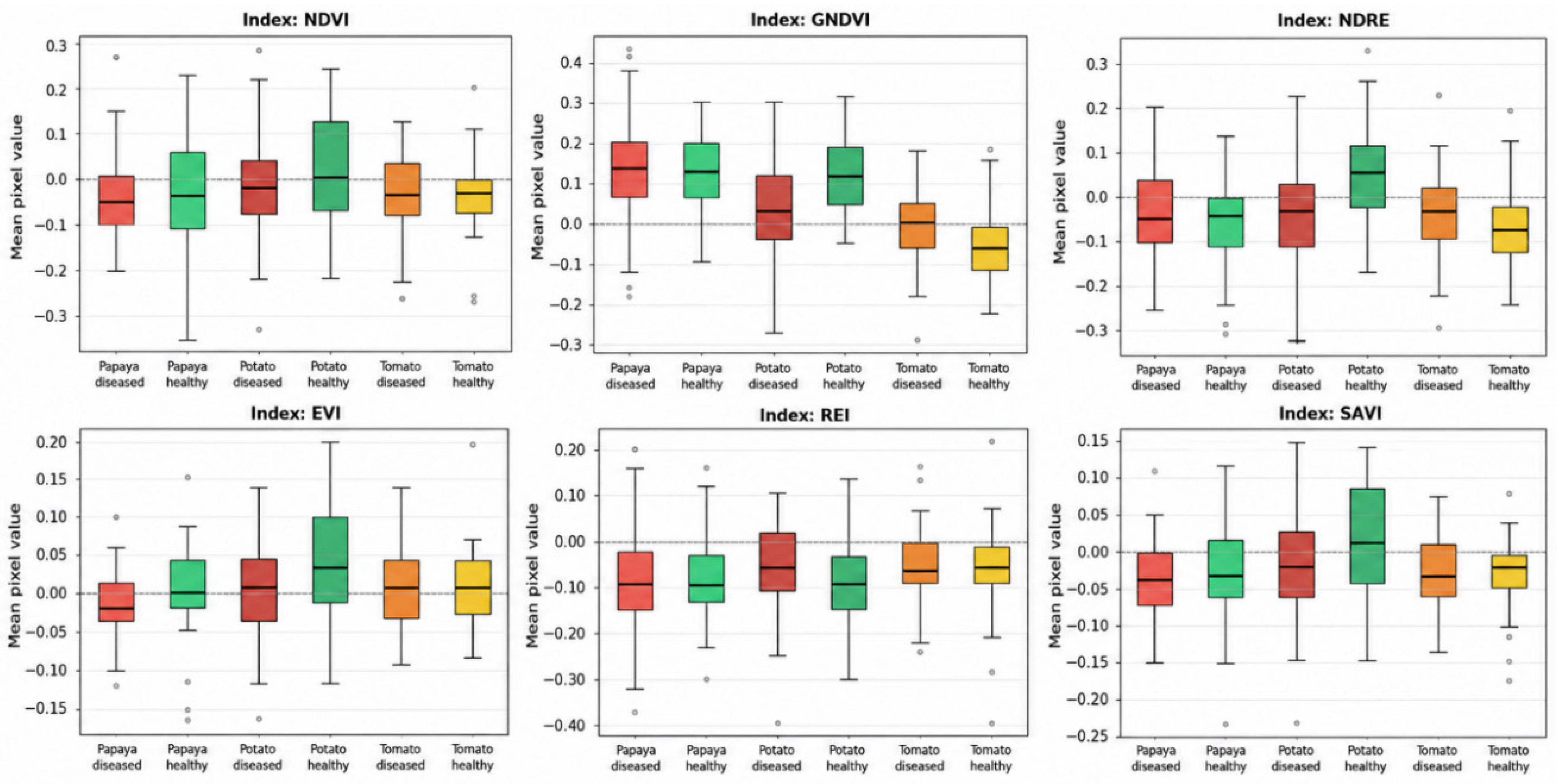
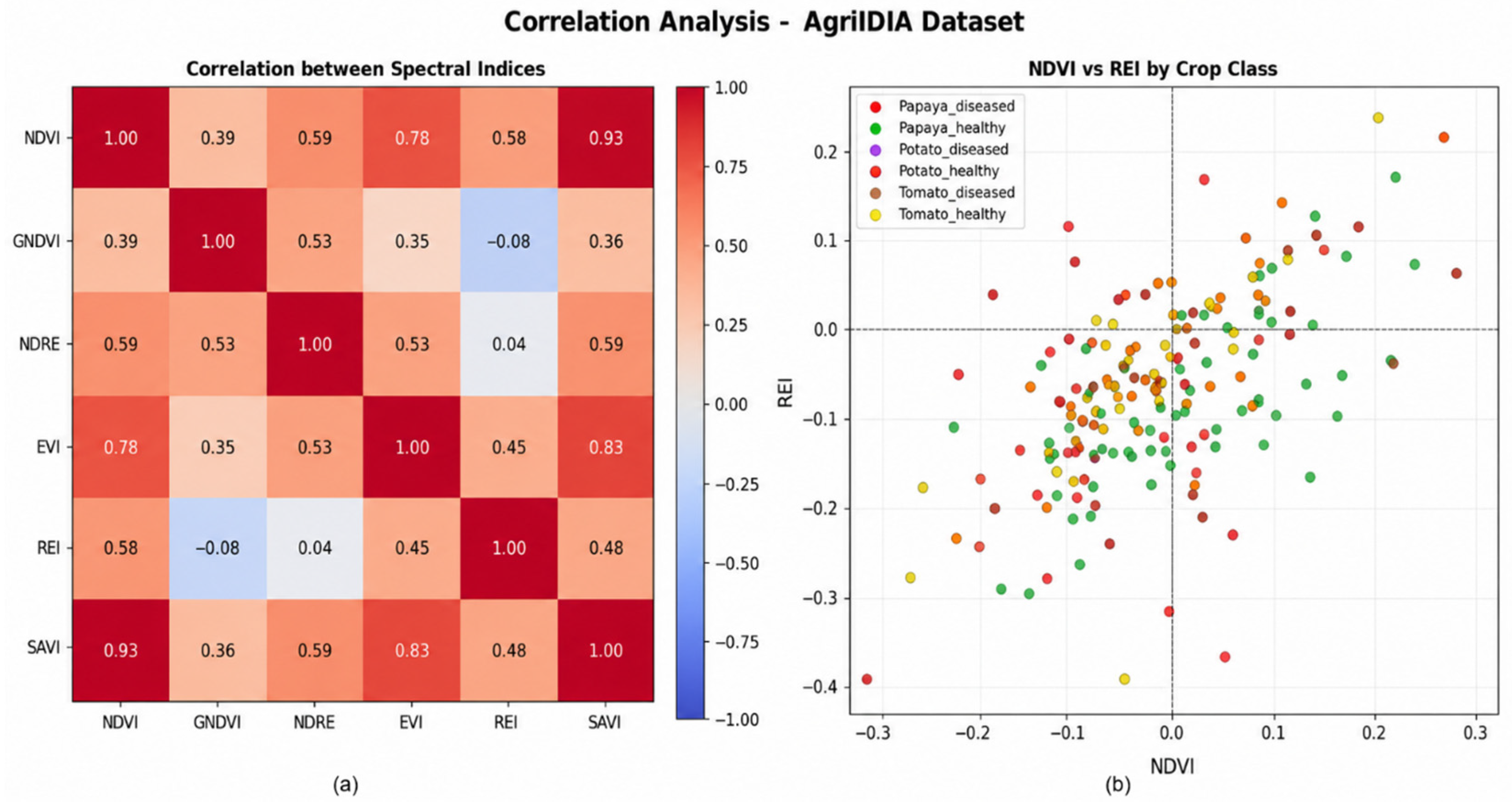
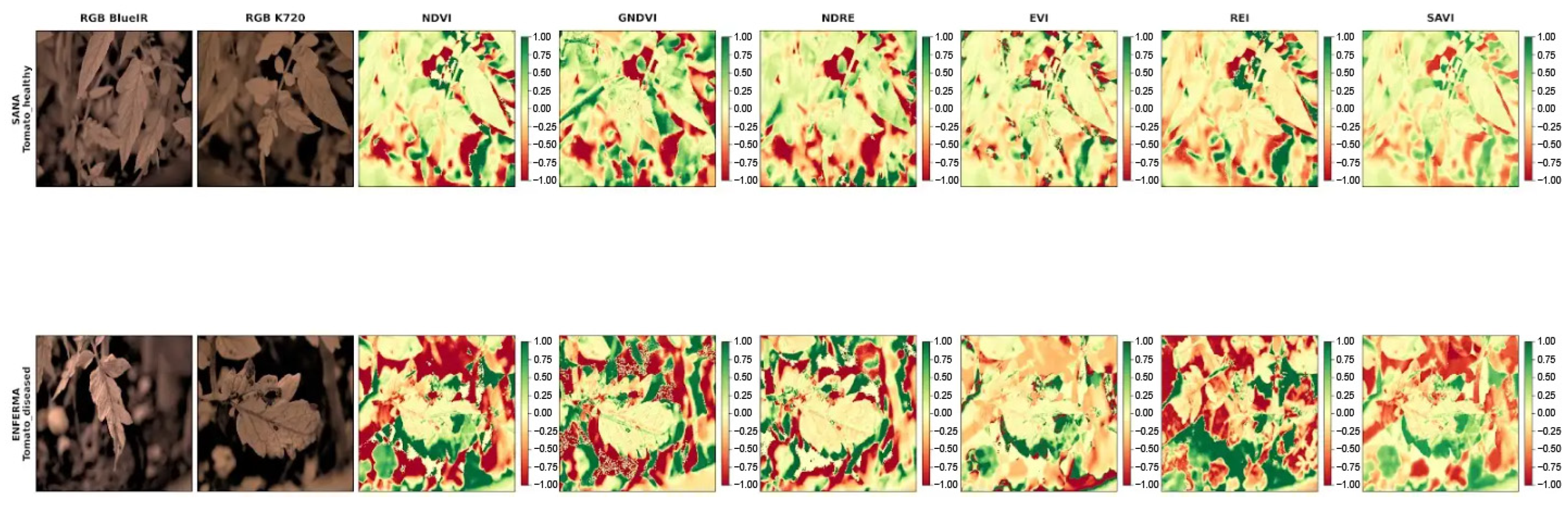
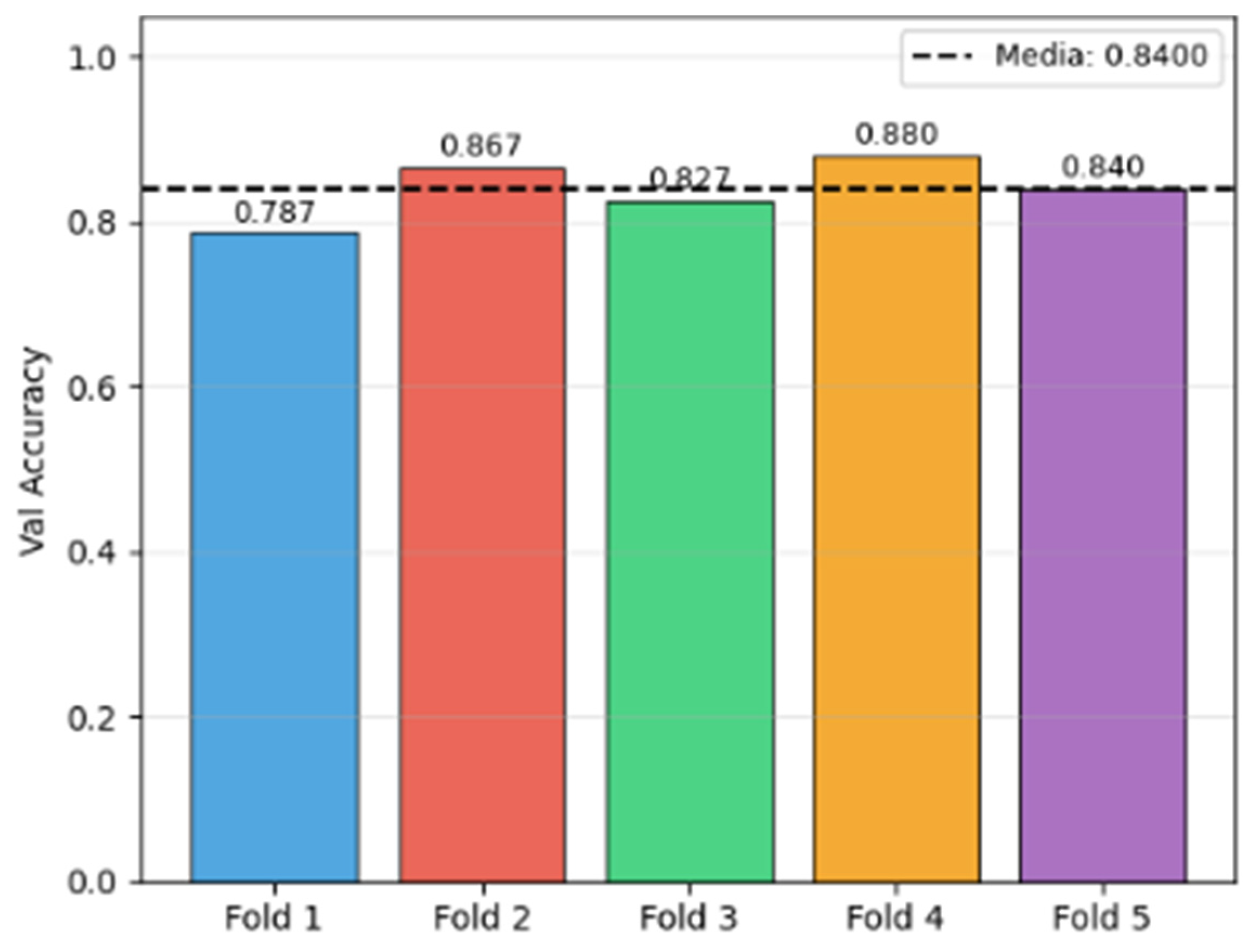
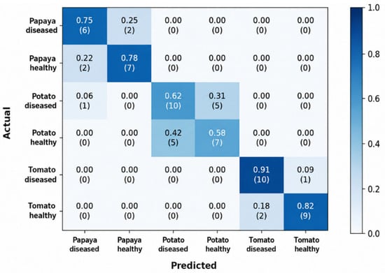
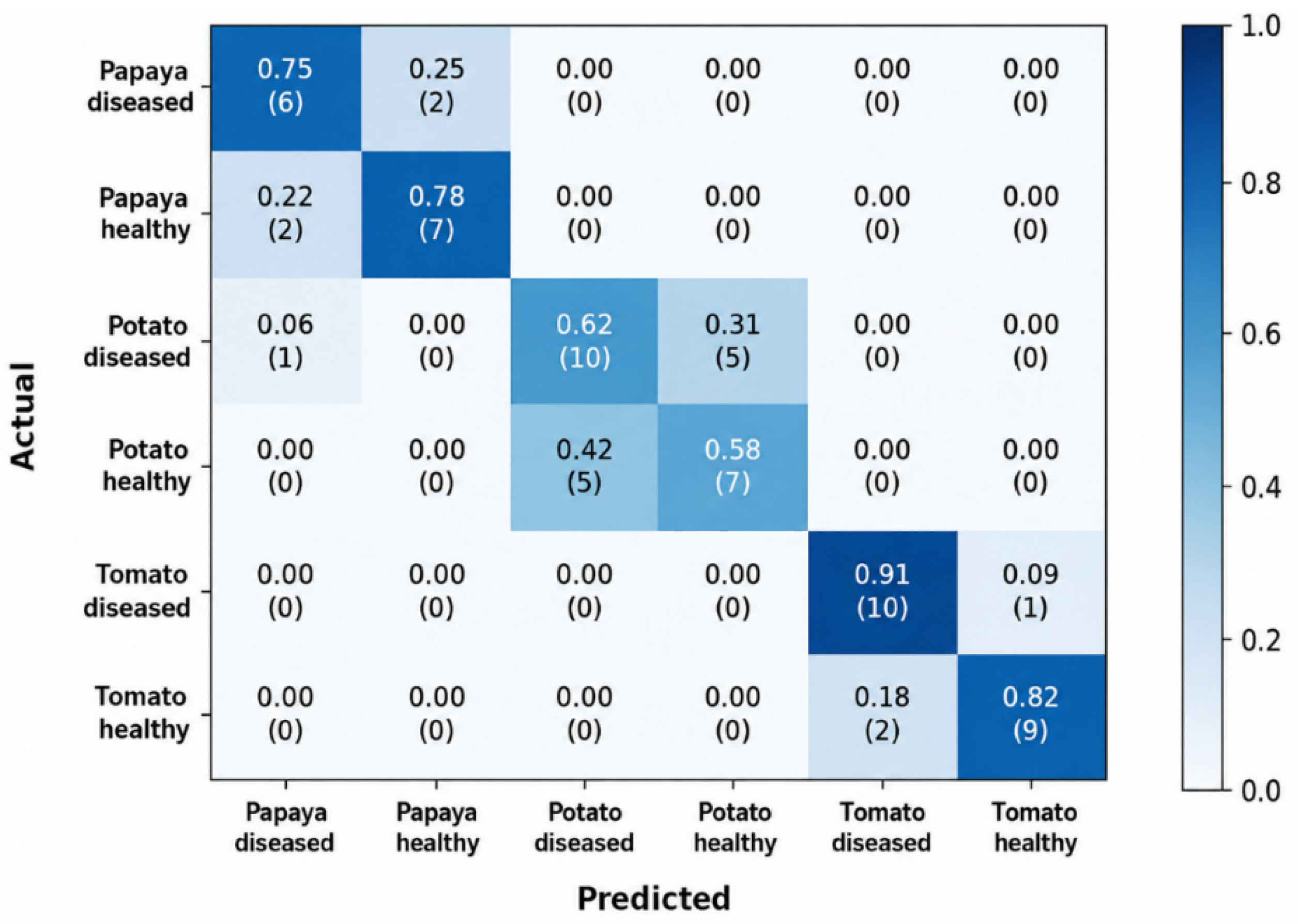
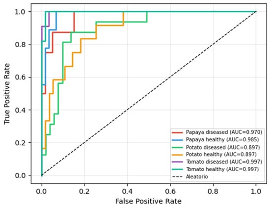
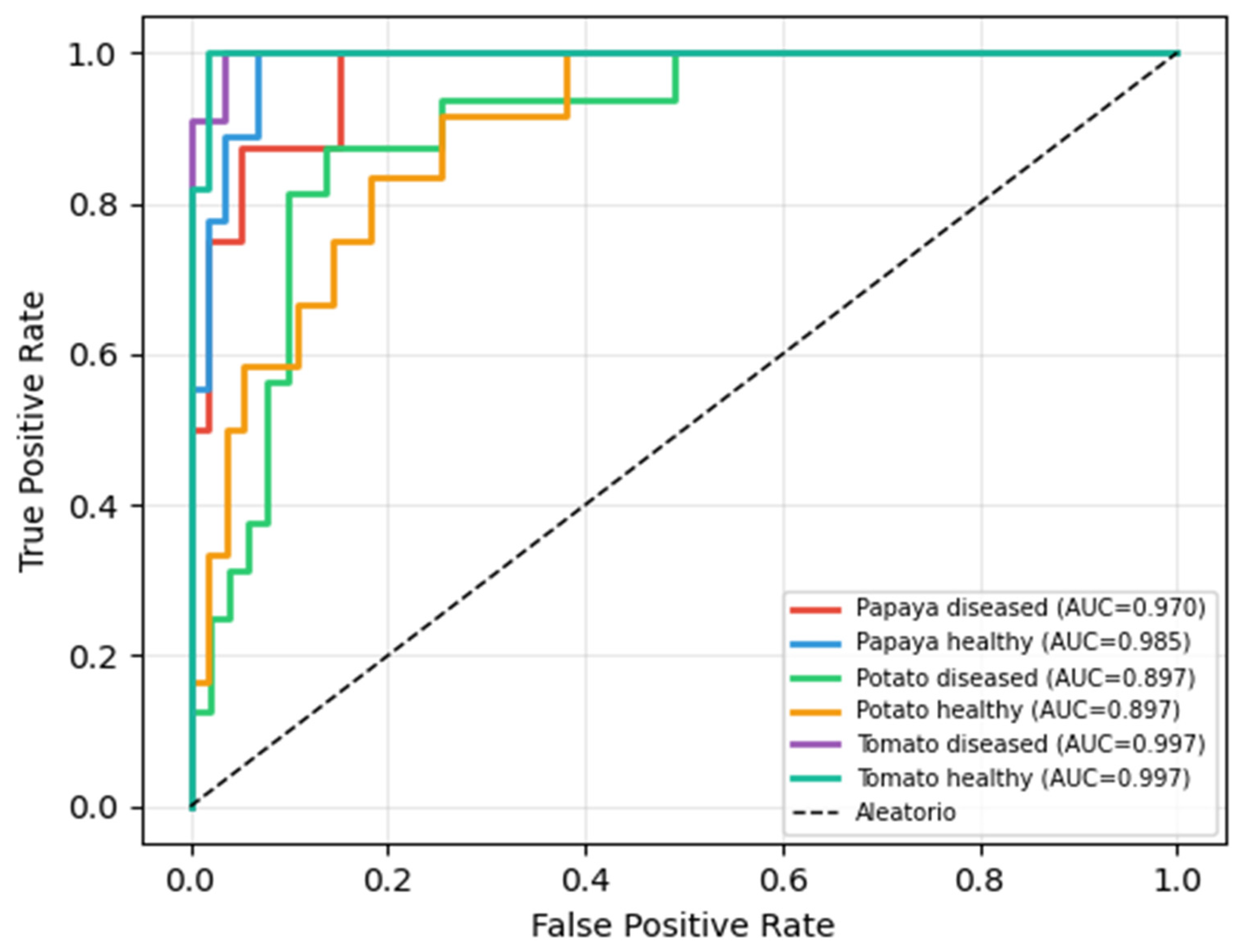

Disclaimer/Publisher’s Note: The statements, opinions and data contained in all publications are solely those of the individual author(s) and contributor(s) and not of MDPI and/or the editor(s). MDPI and/or the editor(s) disclaim responsibility for any injury to people or property resulting from any ideas, methods, instructions or products referred to in the content. |
© 2026 by the authors. Licensee MDPI, Basel, Switzerland. This article is an open access article distributed under the terms and conditions of the Creative Commons Attribution (CC BY) license.