


Abstract
A mobile platform carrying a three-dimensional LiDAR typically uses one localization configuration for a whole mission, yet a horizontal slice of that laser matched against a two-dimensional grid is inexpensive where structure constrains the pose and unreliable in open space and among repeated façades. This paper presents a dual-process system that runs a three-dimensional LiDAR-inertial estimator and a two-dimensional particle filter in parallel and decides at runtime which drives the published pose. The estimates are not fused: one output is selected and the standby channel is throttled rather than stopped, so computation can be separated by mode within one run and compared against a time-aligned baseline. A policy combines four ground-truth-free switching metrics—scan-to-map agreement, particle dispersion, registration fitness and cross-estimator disagreement—through a dwell-time state machine. On three segments of a long-term public dataset, mapped from a different session, the low-compute mode uses 32% and 33% less processor time over the same ground, and in every segment the segment-level planar ATE differs from the three-dimensional baseline by at most 0.084 m. Over a whole traversal the outcome depends on the dwell fraction and on the always-on overhead of both paths: at a dwell fraction of 72% for 0.045 m of added error, +4% at 24%, and +16% when the dwell fraction is zero. Particle dispersion and cross-estimator disagreement carry complementary information about the two ways planar localization fails. The measurements do not indicate that switching is universally beneficial; they show that its trade-off can be measured for a given environment.
1. Introduction
Localization is the stage of autonomous navigation whose failure the others cannot absorb. A planner recovers from a misclassified obstacle and a controller absorbs a modeling error, but neither compensates for a pose estimate that is erroneous and reported as certain, because every subsequent computation is expressed in that frame.
Three characteristics distinguish this work from the adaptive-computation and integrity-monitoring literature reviewed in Section 2. First, existing switching and degeneracy-detection methods either select a mode from one estimator’s assessment of itself or fuse the two estimates into one. Here, the estimators remain separate, one output is selected, and the standby channel is throttled rather than stopped; this is what makes cost and benefit measurable inside a single run against a time-aligned baseline. Second, existing integrity signals are self-assessments, and the failure that matters most leaves them intact, because an estimator that has converged on an incorrect pose with a narrow distribution reports no fault. The pair of metrics used here is chosen so that the two ways that planar localization fails move different signals, and the separation between those distributions is measured rather than asserted. Third, a saving from adaptive computation is usually reported as a single average. The exchange is reported here per environment and against the instantaneous constraint the policy exists to hold, with the dwell fraction at which it breaks even given in closed form, so that the same policy can be shown to reduce processor use in one environment and not in another.
Contributions
We present a dual-process localization system and, more substantially, a measured account of the switch it performs. This study makes three contributions:
Firstly, a pair of switching metrics whose distributions differ complementarily across the two ways that planar localization fails. Four runtime quantities are normalized into two risk scores and combined with asymmetric dwell times. Divergence and confident-but-incorrect convergence move different metrics, and the segment each metric separates is not the segment the other separates.
Secondly, a quantified account of when switching is worth its cost. The exchange between accuracy and computation is reported per segment against the three-dimensional baseline at identical instants, and it differs enough between environments that the same policy reduces processor use in one and does not in another.
Thirdly, an intra-run measurement methodology and a stated observability limit. Computation is separated by mode within one switched run, and each interval is placed against the same simulated instant of a separate baseline run, so cost and benefit are one measurement rather than two averages. The same methodology exposes a limit: when the two estimators share a motion prior, their difference is blind to the error they share.
Three structural mechanisms make the above measurable: a single authoritative publisher of the map-to-odometry transform, so exactly one node writes it in every mode and the standby estimator is throttled rather than stopped; a consecutive-registration agreement gate that breaks the path by which registration error becomes its own input; and a periodic three-dimensional probe, a brief scheduled interval in which the throttled estimator returns to full rate purely so a measurement can be taken. The scope is deliberately narrow: we compare two-dimensional, three-dimensional and adaptive dual modes within one codebase and one platform, and we do not claim the switched output is always the most accurate. Section 5.2 states what bounds each claim.
2. Related Work
2.1. Background: Map-Based LiDAR Localization
In simultaneous localization and mapping (SLAM) the platform builds a map of an unknown environment while tracking its pose within it [1,2]. In map-based localization the map already exists—from an earlier SLAM session, a survey or a building plan—and the task reduces to determining where the platform is inside it. Such a map, fixed before the mission and not modified during it, is a prior map, and it is what both estimators here match against. Light detection and ranging (LiDAR) dominates this task because it measures geometry directly and is far less sensitive to illumination than passive cameras, but a modern spinning unit returns tens-of-thousands to millions of points per second, and that data rate is the origin of the problem addressed here: the geometric richness that makes three-dimensional matching accurate is the same richness that makes it expensive.
The dominant architecture separates the estimate into a fast local part and a slow global part. The fast part is odometry, accumulated between successive measurements; it is smooth and always available, but its per-step errors accumulate without bound, a growth called drift. LOAM established the modern pattern, pairing a high-rate odometry thread with a low-rate mapping thread [3]; later systems coupled the LiDAR to inertial measurement, either in a factor graph [4] or in an iterated error-state Kalman filter (ESKF) that estimates the small error of a nominal trajectory and holds the map in an incremental k-d tree [5], the kind used here. Where a prior map is available, a further component aligns the locally consistent estimate to it. That alignment is registration, performed most often by iterative closest point (ICP) [6] or the normal distributions transform (NDT) [7], and its output is a correction between the map frame and the odometry frame. That correction is nominally quasi-static, changing only as slowly as the odometry drifts, and that expectation is what later makes it usable as a switching metric.
A considerably older approach reduces the problem to the plane. A single horizontal ring of range measurements is matched against a two-dimensional occupancy grid, and the pose is represented by weighted samples, called particles, that a motion model moves and a measurement model re-weights [1,8,9,10]; KLD-sampling reduces the particle count when the posterior is compact [11], and adaptive Monte Carlo localization (AMCL), used here, operationalizes that family on a grid of the type produced by planar SLAM systems [12,13]. Its appeal is cost: the state is three-dimensional rather than six-dimensional, the map is an image rather than a point cloud, and the measurement update touches a few hundred beams rather than tens-of-thousands of points.
The approach carries a geometric assumption. A horizontal cross-section at the sensor’s height must contain enough distinctive structure to constrain the pose in the plane. Where it does, the sample cloud contracts around the true pose within a few updates. Where it does not, the same algorithm continues to run and continues to report an estimate. What the filter’s covariance measures is then worth stating precisely: it describes the spread of the posterior, not the accuracy of its mode, so a narrow distribution can accompany a pose that is wrong.
2.2. Two Failure Modes and the Limits of Self-Assessment
Whether the planar assumption holds is strongly correlated with whether the platform is inside a building. Interiors present walls, doorways and corridor ends at roughly sensor height, and satellite navigation is unavailable, so planar LiDAR localization is both feasible and necessary. Open outdoor spaces present the opposite: the horizontal slice returns few points, and those it returns lie far away and are nearly parallel, so the measurement constrains the pose weakly in at least one direction. Work on degeneracy in optimization-based state estimation describes this in terms of the conditioning of the problem [14]: some directions of the state receive little constraint from the geometry, and the estimate along them is governed by the motion model alone.
Less often stated is that this is only one of two ways the planar estimator fails, and that the two look nothing alike from the outside. Where constraint is absent the sample cloud spreads, the filter’s own report of its uncertainty grows, and a monitor watching that report sees the failure. Where the environment instead offers structure that repeats—regularly spaced façades, rows of parked vehicles, a colonnade—the measurement model is not weak but ambiguous, and the filter can contract confidently around a pose displaced by the repetition period. This is perceptual aliasing, familiar from place recognition [15], appearing inside the pose filter rather than in a loop-closure module. In that condition the filter’s self-reported uncertainty is small, and a monitor watching only that report sees nothing at all.
The same limitation applies to the three-dimensional path. Registration reports a fitness score, the proportion of points that found a correspondence within a threshold, and it is tempting to treat that as a confidence measure—however, it is not: a registration can align a large fraction of the scan onto a locally similar but globally wrong structure and report an excellent score while doing so. Uncertainty-aware work has shown that indiscriminately accepting map-matching poses reduces reliability where structure is sparse or the environment has changed since the map was built [16]. What this class of quantity measures is internal consistency, and internal consistency is exactly what both failure modes preserve. Any monitor assembled only from quantities an estimator computes about itself inherits that blind spot.
Detecting the second failure mode therefore requires comparison against something the estimator did not produce. This is the familiar argument for redundancy-based diagnosis: running several models in parallel and reading the fault from their disagreement rather than from any one model’s residual [17]. The present work applies that reasoning to two localization formulations differing in map representation, estimator and matching—and therefore in failure mode—in a setting where the platform must keep operating while the diagnosis is made [18].
2.3. Adaptive Computation and the Problem Addressed
That different parts of a route deserve different amounts of computation is not new. Adaptive localization and mapping systems have adjusted sensing rates, keyframe selection or back-end optimization according to navigation demand [19]; benchmarking work has emphasized that accuracy, runtime and energy must be evaluated together [20,21]; and surveys have identified hardware-aware tuning as essential for real-time localization [22]. These studies have motivated adaptation, but they usually optimize a single estimator or a single fused graph. The present work instead maintains two heterogeneous estimators with different failure mechanisms, and it treats the switching decision, the standby computation, the handover continuity and the validity of the switching metrics as one instrumented system.
The difficulty is not that either estimator is inadequate; each is well matched to part of a route. It is that the boundary between the parts is not known at design time, is not marked in the map, and cannot be read from either estimator’s own report of its confidence, so a system committing to one configuration spends computation it does not need for part of the route and lacks the accuracy it does need for the rest. Deciding at runtime requires a signal that distinguishes the two regimes, and the preceding subsection shows that no single self-assessment can.
Table 1 places this work among those approaches by the design characteristics that separate them, and the last three columns carry the distinction this paper turns on. The decision is read partly from a quantity no single estimator can produce, since one of the four metrics is a comparison between two of them. The estimator that is not publishing is slowed rather than stopped, which is what keeps its cost attributable and its handover immediate. And because both modes run inside one execution, the cost of each is measured there rather than inferred from two averages. None of these approaches, this one included, requires ground truth while running; what this work needs it for is the calibration procedure of the Supplementary Materials. The table is a qualitative placement and not a benchmark: no external system was run on this data, and a quantitative comparison would require exactly that.
Table 1.
Design characteristics of the approaches reviewed in this section, as characterized there. Rows follow the order in which the approaches appear above.
3. Materials and Methods
3.1. System Architecture and Measurement Boundary
A platform equipped with a 3D LiDAR and an inertial measurement unit (IMU) moves through an environment for which a prior map exists in two forms: a point cloud for the three-dimensional path and an occupancy grid for the two-dimensional path, both built from a separate session. The task is to estimate the pose in the map frame at every instant, at the lowest computational cost consistent with an accuracy requirement.
The two estimators are not combined into a single filter: the system measures both channels, selects one published pose, and changes the computational intensity of the standby channel. That separation has a methodological consequence the evaluation depends on—because only one channel is published while the other still runs, the cost of each mode can be attributed within one switched run, for which a time-aligned baseline run then supplies the comparison.
The system uses the conventional three-frame arrangement: a fixed map frame, an odom frame in which the LiDAR-inertial estimate is continuous but drifts, and a base frame on the platform. is produced continuously by the front end; is a correction absorbing the accumulated drift, and it is the quantity about which the two paths disagree. A decision that shapes everything downstream is that exactly one node publishes that correction, in every mode: when the three-dimensional path is active it republishes the registration result, and when the two-dimensional path is active it derives an equivalent correction from the particle filter’s pose. Consumers of the transform tree therefore read one chain from one publisher and are never exposed to competing publishers or to a conflict between reference frames. This is a statement about publication authority, not about the continuity of the pose itself, which Section 4.1 measures separately.
Figure 1 draws both the architecture and the state machine. The inactive path is throttled rather than stopped (Section 3.5). This costs resident memory, since the standby estimator holds its map, and it buys handover without restart: a transition changes which estimate is published rather than starting a process. Instrumentation is kept separate from policy: a dedicated node subscribes to both paths, performs the temporal association and staleness handling once, and publishes a synchronized snapshot of the switching metrics, so the policy consumes a single time-stamped record and contains no interpolation logic of its own:
Figure 1.
Architecture of the dual-process localization system (a) and the mode state machine that drives it (b). In panel (a), blue marks the three-dimensional path and green the two-dimensional one; red marks the three nodes this work adds, and grey the unchanged upstream and downstream nodes. Dashed arrows carry mode and control topics, solid arrows carry data. In panel (b), the same blue and green identify the mode in which each path publishes.
3.2. Switching Metrics
Several quantities are computed continuously while the platform drives. We call them switching metrics: each describes how well an estimator is currently working rather than what it estimates, and all are available without ground truth. Not all enter the decision, and the distinction matters for reading Section 4.3; Table 2 gives their roles.
Table 2.
Role of each switching metric in the policy and the gate.
Scan-to-map agreement is the fraction of points in the current planar scan whose nearest occupied grid cell lies within 0.4 m, with the scan placed in the map by a pose. It is computed twice per tick from the same scan, grid and radius, differing only in which pose places the scan: uses the particle filter’s pose and the three-dimensional estimator’s. The pair asks one geometric question—is the platform seeing what the map says should be here—of each estimator’s answer in turn.
Particle dispersion is the square root of the larger horizontal eigenvalue of the position covariance reported by the particle filter, a distance in meters summarizing how far apart the filter’s hypotheses are. Its behavior under the two failure modes is opposite, which is the property the policy exploits: it grows when constraint is absent and stays small when the filter converges on an aliased pose.
Registration fitness is the inlier ratio returned by prior-map registration at its correspondence distance of 1.0 m, computed from the voxel-downsampled three-dimensional scan against the cropped map and published once per registration. It resembles in form but differs in every other respect, agreement being computed outside the registration and not depending on it having run. We use f as an availability proxy rather than as a measure of integrity: it indicates that registration converged, not that the pose it converged on, is right.
Cross-estimator disagreement d is the planar distance between the two pose estimates computed by different means,
where is the particle filter’s pose, and where the bracketed term is the three-dimensional estimate expressed in the map frame by composing the most recently adopted registration correction, held by zero-order hold, with the current odometry. The bracket with subscript takes the planar components of that composed pose, since d is defined in the plane. Only adopted corrections enter d: the node computing it subscribes to the correction the agreement gate of Section 3.4 published, so a rejected registration is never used. The quantity is evaluated at each particle-filter timestamp.
The distinction between d and the other three is central to this paper. The first three are self-assessments, each estimator grading its own work and each therefore preserved intact by a failure that leaves the estimator internally consistent. Only d compares two channels built on different map representations, estimators and matching formulations. The two are heterogeneous in formulation rather than in sensing (Figure 2), which is the limitation that Section 5.1 develops.
Figure 2.
Sensor configuration of the recording platform (a) and the sensor streams this work read (b). Red marks the two sensors this work read, blue the three-dimensional path and green the two-dimensional one. Heights were in the body frame, whose origin was the center of the wheel axle; in the frame that the cloud was published in, the laser sat 1.03 m above that origin, about 1.45 m above the ground. The photograph in (a) is from [23].
A fifth quantity, the registration step j, is the planar distance between consecutive registration results. It drives the agreement gate but carries no policy weight, and it depends on the interval between registrations, so comparisons of j are meaningful only at a fixed rate.
Each metric carries the timestamp of the measurement it was computed from, and the elapsed time since is the metric’s age. A metric whose age exceeds a per-metric limit is excluded from the current decision rather than held at its last value, which would silently present old evidence as current.
3.3. Risk Normalization and the Switching Policy
The policy has one objective, stated here because Section 4 judges it against this and nothing else: keep the planar error of the published pose below the instantaneous error limit while spending as little computation as possible. The two halves are not symmetric. The limit is a constraint to be satisfied, and computation is minimized subject to it, so a policy that saves computation while exceeding the limit has failed, and one that holds it without saving anything provides no computational benefit.
Each metric is mapped onto a normalized risk contribution in [0, 1], where 1 indicates the highest risk. In each pair of bounds the reference value is the one at which the contribution is zero, and the other is the value at or beyond which it saturates at one: and are the agreement and fitness that a healthy channel reaches, while , , and are the values treated as fully alarming. The mapping exists because the four metrics carry different units and differ in scale by orders of magnitude, so a weighted mean of them is meaningless until each is expressed on a common dimensionless axis on which one denotes fully alarming. It is a clipped ramp rather than a calibrated probability because the policy compares the result against a threshold and never multiplies it by anything: what has to be right is the ordering between instants and the two values at which a metric stops carrying information, which is what the bounds of Table 3 fix. Writing clip(x) = min(max(x,0),1),
Table 3.
Key parameters used in the evaluation.
Particle dispersion is normalized logarithmically because a covariance eigenvalue moves multiplicatively: across environments its median varies by more than an order of magnitude, so on a linear scale the open-space value saturates the interval, and every distinction below it is compressed toward zero.
The two risk scores are weighted means over the metrics valid at that instant. Let be the set of metrics whose age is within the limit of Table 3, let M be the three metrics entering , namely , and d, and write for the normalized contribution of metric i, that is , or above, and for its weight, given in Table 3:
is undefined when none of its three metrics is fresh, exactly when f is stale, and either is propagated as a missing value rather than a zero: re-normalizing by the weights actually present means that losing a metric reduces the resolution of the estimate instead of biasing it, whereas substituting zero would drift toward declaring everything safe as the inputs went stale.
The policy is a two-state machine with asymmetric dwell times, a dwell time being the minimum interval for which the transition condition must hold before the mode changes. Rising to the three-dimensional mode requires one second of sustained evidence, falling back requires five. The asymmetry encodes the asymmetry of the consequences: being in the high-compute mode unnecessarily costs computation, which is recoverable; being in the low-compute mode wrongly costs accuracy, which is not. Evidence must be contiguous, so an intermittent condition resets the timer rather than accumulating toward a transition.
Two independent paths can raise the mode. The first is exceeding . The second is a direct trigger on the rolling median of d over a ten-second window, which raises the mode regardless of the weighted score. The separate path exists because d is the only cross-validating signal in the set: buried inside a weighted mean, two healthy-looking self-assessments can outvote it, which is exactly the situation in which its contribution is most valuable. Raising the mode additionally requires the three-dimensional path to be available, ; otherwise the transition is blocked and the condition logged.
On every transition into the two-dimensional mode the particle filter is re-seeded from the three-dimensional pose with a small fixed covariance. Without this the filter would resume from whatever belief it held while inactive, which in an environment where planar localization fails is a diverged one.
Algorithm 1 states the policy. Its persistent state is the current mode, the timestamp at which the present candidacy began, and the window of recent d samples. Note line 22: evidence must be contiguous for the dwell time to elapse, so an intermittent condition resets the timer rather than accumulating toward a transition, and line 24 is the re-seeding just described.
| Algorithm 1 Switching policy, evaluated once per metrics snapshot |
| State : mode in {2D, 3D}; t_cand (or none); D (window of d) Input : snapshot S at t with a_2D, sigma_d, f, d and timestamps Output: mode, transitioned 0 transitioned <- false 1 M <- normalize(S) > retain fresh metrics only 2 if S.d is newer, append it to D drop entries older than t - W_d 3 d_med <- median(D) if |D| >= n_min else none 4 R2D <- weighted_mean(M, {w_a, w_sigma, w_d}) > none if no metric is valid 5 R3D <- M.f > none if f is stale 6 7 if mode = 2D then 8 cand <- R2D != none and R3D != none 9 and (R2D > theta_on or (d_med != none and d_med > d_trigger)) 10 and R3D < theta_ok 11 dwell <- t_up ; next <- 3D 12 else 13 cand <- R2D != none and d_med != none 14 and R2D < theta_off and d_med < d_release 15 dwell <- t_down ; next <- 2D 16 17 if cand then 18 if t_cand = none then t_cand <- t 19 if t - t_cand >= dwell then 20 mode <- next ; transitioned <- true t_cand <- none 21 else 22 t_cand <- none > evidence must be contiguous 23 24 if transitioned and mode = 2D then reseed_2D(pose_3D) 25 return mode, transitioned |
3.4. The Consecutive-Registration Agreement Gate
Registration does not match against the whole prior map. Before each attempt a local region is extracted around the current estimate, and each result therefore becomes two things for the next one: its initial guess, and the center of the region of the map it is allowed to see. This closes a loop in which a bad correction places the next registration in a worse starting position and lets it see the wrong part of the map, producing a worse correction. The consequence is observable directly: without the gate, a transform that should be quasi-static moves by meters every few seconds and wanders over a range comparable to the size of the segment, at a drift rate approaching the platform’s own speed.
The remedy is a consistency check on the loop’s input. A correction is adopted only if it passes the fitness floor and agrees, within , with the previous qualified registration taken at least earlier. A single registration may be wrong, but two registrations performed on different data landing on the same wrong answer is a less likely event. Only qualified results become references, and the adopted transform—never a rejected candidate—is what seeds the next initial guess and crop center; the first correction of a run is exempt. The idea is related in motivation to uncertainty-aware acceptance of map-matching poses [16], but the criterion is agreement between consecutive qualified registrations rather than fitness alone. Its scope should be read from that definition: it compares the planar translation of consecutive corrections and nothing else, so a correction wrong in yaw or in height while agreeing in xy passes it, and two registrations converging on the same wrong pose agree by construction—the case repeated façades are most likely to produce, and the environment the gate is least able to protect. What the gate guarantees is therefore narrow and is worth stating precisely. It enforces planar consistency between the two candidate registrations used in the qualification test; it does not bound the step between consecutively adopted map-to-odometry transforms, which Section 4.1 measures separately. It is not a test of whether a pose is right, it constrains neither yaw nor height, and it cannot separate two consistent registrations from two consistently wrong ones. Extending the check to full SE(3) consistency, and to a reference the registration does not itself produce, is left to future work.
3.5. The Standby Channel: Throttling and the Periodic Probe
While the two-dimensional path is active, the three-dimensional channel is slowed in two independent places, and the saving reported in Section 4.2 is the sum of the two.
The first is the front end, which skips the LiDAR measurement update on all but every N-th scan, propagating on inertial data in-between; we call N the stride. In an ESKF the propagation step is inexpensive, whereas the update step associates every retained point with the map, forms the residuals and solves the resulting system. Skipping updates therefore reduces cost with the stride, though not in proportion to it, because propagation and point preprocessing continue at full rate and set a floor.
The second is prior-map registration, whose rate is a property of the mode: while the three-dimensional path drives the output the system re-registers at , and on standby at the lower , since there it is kept running only to hold the switching metrics alive and the age limits of Section 3.2 set how slow it may become. This is the larger of the two savings in relative terms, registration falling from 25.6 to 6.0% of a core in indoor, though in absolute terms the front end gives up more.
Throttling has a failure mode that has to be bounded. Between updates the state covariance grows, so when an update arrives the filter weights the LiDAR heavily relative to its prediction; where the LiDAR constraint is weak that single update can be badly wrong, and the wrong state seeds the next registration. In outdoor_a, the most open segment, a stride of four makes the three-dimensional odometry diverge outright, at apparent speeds two-orders-of-magnitude above the platform’s, and a stride of two is required there. The general statement is worth keeping separate from that value: in a dual-process design the standby saving must come from lowering the rate of the expensive operations while the inexpensive ones continue, so the estimator is slowed rather than suspended. The two settings are bounded in opposite directions—the stride cannot be too large, the registration rate cannot be too low—and both depend on the environment and the estimator configuration together.
Throttling also prevents the cross-validating metric from being observed, because d depends on the three-dimensional estimate. To bound the interval over which that signal is unavailable, the system releases the throttle on a fixed schedule; we call one such release a probe. Every , for a duration , the three-dimensional front end runs at full rate, and only d samples from inside that window—plus a grace period during which the quasi-static correction remains trustworthy—are passed to the policy. The published pose remains the two-dimensional estimate throughout, so the probe is instrumentation, not a mode change, and its cost is the cost of observing rather than of switching. That cost is the duty cycle multiplied by the per-mode difference in processor use, so the schedule is a design parameter whose price is computable in advance.
The same schedule fixes how long a fault can go unobserved, which is the quantity an application requirement has to be checked against. Disagreement exists only inside a probe window and its grace period, so a fault that appears just after one closes waits the blind interval for the next; the rolling median is then undefined until samples have arrived, which takes ; and the transition is taken only after the dwell time . The worst case, written , is their sum:
The middle term is bounded by the probe window rather than by , since d exists only inside that window and its grace period: cannot exceed , and in practice it is far shorter, the samples arriving within one second at the rate the particle filter publishes. With the values of Table 3 the blind interval is 12 s, the dwell 1 s, and the worst case therefore lies between 13 and 21 s. A platform traveling at speed v covers in that time, so the schedule holds a one-meter requirement against a fault whose error grows no faster than the platform travels only for v below , which is 0.08 m/s at best. Read as a design rule the inequality inverts to : bounding the worst case at a walking speed of 1 m/s would require a period below 8 s and a duty cycle above 60%, which would spend most of the saving the standby mode exists to produce. We verified the schedule rather than optimizing it, and we record that this bound is not met at the speeds of this dataset. The assumption behind it is itself optimistic: a diverging planar filter can move faster than the platform does.
The same tension motivates adaptive triggering in networked control, where the detection cycle is shortened in response to the error observed in the previous cycle instead of being held fixed [24]. The analogue here would drive from the disagreement observed in the last probe, but the quantity driving the adaptation there is a measured error, which is exactly what this policy does not have at run time.
Table 3 lists the parameters used in the evaluation, classified by what kind of quantity each is, which determines whether it must be re-established for a new environment. A statistical scale is read from the distribution the metric takes in the target environment, and it is the only kind the calibration rule of Section 5.2 produces; an implementation scale is set by the sensor and the registration implementation; an operating choice is set by the designer from the application requirement; a structural value is an algorithm constant. The standby stride is listed separately because it is not a scale at all: setting it too aggressively can make the three-dimensional estimator diverge rather than merely degrade, so it is bounded by stability and not by a distribution.
Two entries deserve comment. The active re-registration rate is the same in every environment, a simplification made possible by the agreement gate; before the gate, the two environment types required rates more than an order of magnitude apart. And the standby stride is environment-dependent, which is a limitation of the present configuration rather than a property of the design: both values were established offline from the stability limit of the three-dimensional estimator, and a deployment without that information would have to adopt the smaller of the two and accept the smaller saving. Although we did not run that configuration, the resulting reduction in the saving can be bounded from the cost structure. The front-end saving comes from skipping the LiDAR update on all but every N-th scan while propagation and point preprocessing continue at full rate, so the update cost falls roughly as 1/N toward a floor set by the part that never stops. Moving from a stride of four to a stride of two therefore returns about half of the update cost that was being saved rather than half of the mode’s total, and the registration saving is untouched, since it is governed by and not by the stride. Because registration is the larger of the two savings in relative terms, a conservative single stride keeps the larger part and gives up a fraction of the smaller one. This is a bound read from the cost structure, not a measurement.
3.6. Dataset, Segments, Platform and Protocol
We used the University of Michigan North Campus Long-Term (NCLT) dataset [23], which provided synchronized LiDAR, inertial, wheel-odometry and ground-truth data recorded repeatedly over a campus containing both building interiors and open outdoor areas. Its multi-session character is what made it suitable: the localized run was the 20 August 2012 session and the prior maps were built from the 17 November 2012 session, about three months apart. Building a map from the session that was subsequently localized measured the registration of a point cloud against itself and produced optimistic figures that did not transfer to deployment.
Figure 2 draws the recording platform and the streams that this work read. Of its sensor suite, we used two: the Velodyne HDL-32E at 10 Hz (Velodyne LiDAR, Morgan Hill, CA, USA) and the Microstrain inertial unit at 100 Hz (LORD MicroStrain, Williston, VT, USA). The three-dimensional path consumed both; the two-dimensional path consumed a planar slice extracted from the same cloud rather than the platform’s own planar scanners. The two estimators therefore shared one sensor and one motion prior, and they differed only in the map representation and the matching applied to it. The RTK receiver supplied ground truth alone; the cameras and the planar scanners were not read.
Three segments were selected to span the failure modes of Section 2.2: an indoor passage (indoor), an open road (outdoor_a) and a courtyard bounded by repeated façades (outdoor_b). Table 4 summarizes them. The first seventy-five seconds of each window were excluded from scoring: the initial pose was injected 45 s after the segment started, and scoring began a further 30 s of warm-up after that, so the scored windows were 145, 125 and 95 s long.
Table 4.
The three evaluation segments.
All three segments were windows of the same recorded session. Map coverage was the fraction of the segment’s path that fell within the extent of the prior map; it is not reported for indoor, part of which passed through a building interior for which that quantity was not meaningful.
In Figure 3, occupied cells are dark, free cells are white, and cells that the prior map never observed are light gray, with the dashed line marking the edge of that map. Each grid is shown in its own frame, unrotated, and the whole segment window of Table 4 is drawn with the excluded first seventy-five seconds in gray. The three panels are the premise of Section 2.2 made visible: what a horizontal slice at sensor height has to work with differs between them, from walls and doorways, through a road section that returned few points, to façades that repeated.
Figure 3.
The prior occupancy grid of each evaluation segment with the ground-truth trajectory drawn over it.
Ground truth was expressed in a campus-wide frame. A rigid transform aligning each prior map to that frame was estimated once per segment and held fixed for all runs, rather than re-aligning each trajectory during evaluation; the residuals of those three alignments were 0.321, 0.329 and 0.296 m RMS. This was not a floor on achievable accuracy—the three-dimensional baseline reached 0.206 m, below it—because a fixed frame offset displaced every mode alike and partly canceled in a comparison between them. What it bounded was the meaning of an absolute number.
All runs were executed on one machine, an Intel Core i7-10750H at 2.60 GHz (Intel Corporation, Santa Clara, CA, USA) with 6 cores and 15 GiB of memory, running Ubuntu 20.04 and ROS Noetic with the governor fixed to performance and visualization disabled. The two-dimensional path used the amcl package of the ROS navigation stack, version 1.17.3. Processor use was sampled per process at 0.5 s by a node that excluded itself, the launcher, the ROS master and the log playback, and percentages were relative to one core. Two measured properties bounded how they should be read: playback kept real time to within 4.4 parts in one hundred thousand across all twenty-seven executions, and the largest instantaneous total in any run was 41.6% of the twelve logical threads, so the savings were differences in work performed rather than deferred under contention. We report processor use, not energy.
The planar scan was not a sensor output: it was extracted from the three-dimensional cloud by keeping the points inside a horizontal band and projecting them, so the band was a parameter of the baseline rather than a property of the platform. Every run of the primary evaluation used the same band, 0.5-to-0.7 m in the body frame. The laser was mounted inverted on this platform, so the vertical field of view of the recorded cloud ran from 10.67 degrees below the horizontal to 30.67 degrees above it, and the body-frame origin lay 0.36 to 0.46 m above the ground across the three segments. That band therefore cut 0.86-to-1.16 m above the ground, inside the 0.3-to-1.5 m band above local ground from which the occupancy grid was built, so every return it admitted had a counterpart in the grid; the single downward beam first reached the ground near 8 m, so no band considered here contained a ground return. An earlier setting widened the band to 0.0-to-1.2 m in outdoor_a and 0.2-to-1.2 m in outdoor_b for the standalone planar runs alone. Those six executions were repeated with the band matched, and the repeated values are the ones reported here; the earlier configurations of Section 4.3 were not repeated, and Section 5.2 measured what that left. The particle filter used 500-to-5000 particles on a 0.1 m grid with both recovery weights set to zero, so a diverged filter recovered only through the re-seeding of Section 3.3.
Each configuration comprised three segments × three modes (2D-only, 3D-only, dual) × three repeats, twenty-seven runs. The initial pose was injected at an identical offset from the segment start in every mode; without this the modes satisfy their readiness conditions at different times—we measured nearly thirty seconds and forty-five meters of travel—and every cross-mode comparison inherits it. Because all three modes replayed the same log they shared a common clock, so any instant of one run could be compared with the same instant of another, which is what made the trade-off analysis of Section 4.2 possible. The accuracy, computation and memory results came from this primary evaluation; those of Section 4.3 came from earlier configurations that shared the switching implementation but differed in probe setting and were never pooled with it.
One application requirement was fixed here, before any measurement. We took one meter of planar error, of the order of the platform’s own footprint, as the value above which the published pose was unusable. The same number was applied in two ways that were not equivalent: the instantaneous error limit asked whether the error at a given moment exceeded one meter, labeling individual samples and defining the constraint in the policy objective, while the segment-level RMSE threshold asked whether an environment’s planar ATE over a whole segment did, producing the suited and unsuited labels. An environment could satisfy the second while failing the first for part of a traversal: indoor had a planar ATE of 0.423 m yet exceeded one meter at 2.5% of instants. For evaluation here, only zero exceedance in every repeat counted as satisfying the objective.
Accuracy was absolute trajectory error (ATE) on the horizontal plane, reported as RMSE and computed in the frame of the prior map. The planar restriction and the map frame were both required for the measurement to be meaningful. The planar restriction was needed because the two-dimensional filter published zero altitude by construction, so a three-dimensional metric charged its output the entire vertical offset between platform and map origin: in one indoor run the same trajectory scored 5.791 m in three dimensions and 0.457 m on the plane. The frame mattered for the same reason: the mapping session drifted vertically and the rigid alignment represented part of that trend as a tilt, so transforming into the ground-truth frame and only then dropping z would rotate part of the missing altitude onto the horizontal plane. The map frame avoided this and was where the grid, the filter, the registration and every switching metric were defined; substituting ground-truth altitude before transforming reproduced the map-frame values to within 4% in all nine segment-by-mode combinations.
4. Results
4.1. Accuracy and Switching Behavior
Unless stated otherwise, the values are medians of three repeats, with the range in parentheses. A repeat was a repeated execution of the same recorded segment, not an independent traversal: the three shared one log, so their spread measured run-to-run reproducibility rather than environmental variability.
The agreement gate was a precondition for everything else, because without it the three-dimensional path was not reliable enough to serve as the reference against which the policy compared. In outdoor_a, three-dimensional mode only, prior-map registration without the gate gave a planar ATE of 28.568 and 96.148 m at the fast rate and 0.701 m at the slow one, while with the gate it gave 0.312 and 1.484 m; the ordering reversed and the fast rate became the better. Every condition but the fast ungated one was a single run, so these were directional.
The fast rate with the gate was the best of the four combinations by a wide margin. Before the gate, the two environment types demanded incompatible rates: in indoor the fast rate was necessary to escape poor convergence, while in the open it produced errors of tens-of-meters. With the gate, one rate served all three segments, and the 78% adoption rate established that it did not obtain that result by discarding most candidates.
What the gate compared was a planar distance, while the registration it admitted was a rigid transform in six degrees of freedom, so a correction could be quiet in the plane and large in height or heading. The components that it did not read were not logged, but they could be recovered: the adopted correction was the transform between the two published trajectories, which carried identical timestamps, and it changed only when a registration was adopted. Recovering it that way returned exactly the number of adoptions the node reported in each of the nine runs, so the reconstruction was the adoption sequence itself. Table S1 lists the components.
Two quantities had to be kept apart here. The gate read j, the planar distance between two consecutive candidate registrations, and it admitted the correction when that distance was within ; it did not bound the size of the adopted correction itself, which is why the planar steps of Table S1 reached 1.851 m. What Table S1 reports is the step in the adopted map-to-odometry transform between consecutive adoptions, resolved into its planar, vertical and heading parts.
Read that way, the two unread axes behaved differently. Heading was not a problem here: no adopted correction turned the transform by as much as one degree, and the largest, 0.97 degrees in outdoor_a, displaced a point at 20 m by less than . Vertical steps reached 1.59 m, and among the corrections whose own planar step was within , 13% in indoor and 6% in outdoor_a moved the platform vertically by more than that same 0.5 m. The planar geometry that made the gate work was also what left that axis unchecked.
The planar results of this paper were not affected, because they were measured in the map frame with the vertical coordinate discarded; what the measurement added was that the same pose was not continuous in height, and a consumer using the third coordinate would receive those steps unfiltered. Extending the gate to it cost nothing, since the vertical component was already present in the transform being tested. What this measurement could not give was the counterfactual performance of such a gate, since the components of the candidates that the present gate rejected were not recoverable from the published trajectories, which changed only when a correction was adopted. We did not extend it, and Section 5.2 records the gap.
Table 5 reports the planar ATE of the three modes, and Table 6 reports the switching behavior behind it.
Table 5.
Planar ATE RMSE, median (minimum–maximum) of three repeats. All values in meters.
Table 6.
Switching behavior, reported per repeat.
The switched output achieved a lower ATE than the recorded standalone planar configuration in every segment, by factors of 1.7, 523 and 2.3. All three compared configurations that differed only in mode: the scan-extraction height band was the same in both, so these were differences between two algorithms rather than between two recorded configurations.
The second property, staying close to the three-dimensional estimator, held in all three segments. In indoor the switched output added 0.045 m while spending 72% of the interval in the low-compute mode; in outdoor_b it added 0.084 m at a dwell fraction of 24%. Both margins were a fraction of the 0.296-to-0.329 m map-alignment residual of the experiment itself, so they should not be read as evidence of an ordering or of equivalence.
Those margins are differences between two error statistics computed separately, which leaves open how much of each was shared. The two modes replayed one log, so the difficult stretches affected both: a difference taken instant-by-instant removed that common variation, while a difference of summaries kept it in twice. Table 7 reports the paired form, both trajectories placed on one 2 Hz grid over the interval that they shared by the causal zero-order hold of Section 3.6 and scored in the map frame as elsewhere.
Table 7.
Paired difference between the switched output and the three-dimensional baseline, over the instants at which both were defined. Positive means the switched output was the worse of the two. The interval was the central 95% of 2000 circular block resamples within each run, the block length being the autocorrelation time of the difference; the last column is the per-repeat range.
At a typical instant the cost of switching was a few centimeters rather than the larger difference suggested by the segment-level summaries. The difference between the paired and the segment-level result indicates whether the penalty was spread over the traversal or concentrated in a few excursions. In outdoor_a the median paired difference was m over an interval of between and +0.002 m, and the switched output was worse at 43-to-51% of instants, so the two were not distinguishable there; the summary difference was produced by the one repeat that descended, whose excursion raised its error to 0.538 m against 0.345 and 0.360 m. In outdoor_b the median penalty was +0.012 m with an interval clear of zero, in indoor +0.020 m with one that touched it. The cost of the policy was therefore concentrated in rare excursions rather than spread over the traversal.
Three runs per segment remained three runs, and the resampling was within them, so the intervals say how firmly these replays supported the difference, not how it would have fallen elsewhere. Omitting one run at a time moved the pooled difference between +0.039 and +0.055 m in indoor, and +0.101 m in outdoor_a, and +0.075 and +0.131 m in outdoor_b.
In outdoor_a the switched output added 0.003 m, and it did so by not switching: two of the three repeats made zero transitions and spent none of the scored interval in the low-compute mode. This environment did not reward switching, which is the intended behavior of a runtime decision. It also showed what happens when that determination fails: the one repeat that did descend, for 14% of the interval, scored 0.538 m against 0.345 and 0.360 m for the two that did not, the largest switched error of any repeat in the primary evaluation.
Three things are visible in Figure 4 that summary statistics cannot show. In indoor the switched curve tracked the three-dimensional baseline throughout, including while the policy held the low-compute mode, whereas the planar estimator drifted above the instantaneous error limit once the segment left the building. In outdoor_a the representative repeat never descended, so the switched curve lay on the baseline while the planar estimator sat two-orders-of-magnitude above it. In outdoor_b the switched curve left the baseline at the start of the low-compute interval, rose to the instantaneous error limit, and returned to the baseline the moment the policy left that mode: the error was held rather than accumulated, and it is held for as long as the wrong decision stood. Outside the shaded intervals the switched curve lay on the baseline in every segment, and every departure from it fell inside one.
Figure 4.
Planar error against time for the three segments, on a logarithmic ordinate, timed from the end of the excluded interval; shading marks the intervals spent in the two-dimensional mode.
A switching system is normally described as choosing the better of two estimates, but in outdoor_a something more was happening: the particle filter running inside the switched system scored 5.591 m (5.050–15.332) against 188.194 m for the same filter run standalone over the same instants, a factor of thirty-four, while in the other two segments the difference was small. We tested the re-seeding of Section 3.3 as the mechanism by repeating the nine switched runs with it disabled and nothing else changed: it was not the mechanism. The planar channel then scored 6.002 m (5.940–14.791) against 5.553 m (5.105–15.321) in the re-seeding-enabled arm of the same ablation batch, and the switched output 0.348 m against 0.360 m, both within the spread of three repeats and in every segment. Both figures came from that batch and not from the primary evaluation, whose corresponding value was the 5.591 m quoted above. The choice of correction source was excluded as well, since the particle filter did not consume the map-to-odometry transform and read the same scan, grid, wheel odometry and initial pose in either configuration. The standalone failure was orderly rather than anomalous: all three repeats lost the lock 7-to-8 s after the initial pose was injected and never recovered, which was the absence-of-constraint failure that Section 2.2 attributes to this environment. By what path the co-running three-dimensional path kept the planar filter converged we did not establish, and we report the factor as measured rather than explained.
Because the published pose was one estimator’s output rather than a fusion of both, the mode transition was also a handover, and whether it was visible in the output was a separate question from accuracy over a window. Measuring the step across a transition alone did not answer it, since the platform moved between samples. Each transition was therefore compared against ordinary motion in its own neighborhood: the published planar displacement and yaw change across the transition were set against the median speed and yaw rate over the surrounding two seconds, and the excess was the part of the step that motion did not explain. Samples sharing a timestamp, which the recorder produced whenever the pose was re-published without a new estimate, were collapsed to the last of them; over the nine switched runs this reduced 65,827 records to 12,083 distinct instants. Table S2 lists every transition.
The nine switched runs made 14 transitions, 11 of them inside the scored interval. Over the 11, the median step excess was m and the median yaw excess +0.18 deg, so a typical transition was crossed by a step no larger than an ordinary one. Three exceeded 0.10 m, at +0.160, +0.618 and +2.441 m; all three were returns to the three-dimensional mode, and in each the excess accounted for 86, 55 and 93% of the channel gap at that instant, while the four descents produced no positive excess at all. The asymmetry followed from the policy rather than from the estimators: it descended only while the two channels agreed and returned once they had ceased to, so the gap available to appear in the output was small in one direction and unbounded in the other.
To determine whether a transition was corrective, the published error was compared before and after each one. The transition reduced the planar error in 10 of the 11 evaluated cases. The median planar error over the two seconds before a transition was 0.601 m and after it 0.270 m, and the error fell at 10 of the 11 transitions; the exception was a descent in outdoor_a where it rose from 0.128 to 0.134 m. The largest step, 2.441 m, removed 2.370 m of error. In those cases the step therefore discarded error that the channel being left had accumulated rather than introducing error of its own. A consumer requiring a continuous pose would still have to absorb these steps, which Section 5.2 states as a limit of publishing a selected estimate.
4.2. Computation, Memory and the Measured Trade-Off
Two costs had to be separated: what the system cost while it was in the low-compute mode, and what it cost over a whole traversal. Table 8 reports both. The values were the sums of the per-process means over the scored interval, taken as the median of three repeats, in percent of one core.
Table 8.
Processor use by mode against the three-dimensional baseline at the same simulated instants (left), and over the whole scored interval (right). All processor figures are in percent of one core; pp is percentage points of one core.
It can be seen that outdoor_a had no mode-conditioned entry because only one of its three repeats entered the low-compute mode, so a run-level statistic would rest on a single run.
Read together the two halves say something that the individual numbers do not. While the system was in the low-compute mode it cost about a third less than the three-dimensional estimator would over the same ground, in both segments where that comparison was available. Over a whole traversal that gain was set against a cost paid continuously, because a standby estimator that has been stopped cannot take over. Where the low-compute mode held for 72% of the interval the gain dominated and the traversal was 18% cheaper; where it held for 24% the two roughly canceled; and where the dwell fraction was zero, only the always-on overhead remained.
The saving was concentrated in two processes. The three-dimensional front end fell from 54.3 to 22.2% of a core in indoor because its measurement update was throttled, and prior-map registration fell from 25.6 to 6.0% because its rate dropped with the mode; every other node differed by less than two percentage points between modes. Figure 5 shows the same figures stacked by process group.
Figure 5.
System processor use while in the two-dimensional mode (a) and over the whole traversal (b), stacked by process group.
Resident memory was essentially independent of mode, varying by 1.5% and 0.8% (Table 9). The reason was structural and was anticipated in Section 3.1: the three-dimensional front end was throttled rather than stopped, so its incremental map and the prior point cloud remained resident, and only the growth of the map paused. The system reduced processor use but not resident memory.
Table 9.
Resident memory by mode within each switched run, in mebibytes.
The periodic probe was paid for out of the saving, and its price was predictable in advance as the duty cycle multiplied by the per-mode difference of the throttled front end: where that difference was 36 pp, the prediction met 9.7 pp measured. The period and width were not fixed by that calculation, since they set how long an emerging fault could go unobserved; we verified the schedule rather than optimizing it.
Setting these figures against Table 5 gives the exchange in its complete form. In indoor the system increased planar ATE by 0.045 m and reduced processor use by 13.4 pp of a core over the traversal; in outdoor_b it increased planar ATE by 0.084 m, while the mode-conditioned saving and the always-on overhead approximately canceled, yielding no traversal-level computational benefit. The added error was comparable in the two segments; what differed was entirely the resulting trade-off. The same policy with the same thresholds therefore faced materially different exchanges depending on where the platform was, which is the quantitative form of the argument for deciding at runtime rather than at design time. The added error was concentrated in the low-compute intervals: in high-compute intervals the switched run tracked the baseline to within m with a single exception, so the loss is attributable to the policy’s decisions rather than to the switching machinery.
Table 8 also answers a question that can be put to the policy before a mission rather than after it: how much of a traversal must be spent in the low-compute mode for the exchange to pay at all. Writing and for the processor use of the switched system in each of its two modes and for the baseline over the same ground, the switched cost at a dwell fraction D is , and it falls below above a break-even dwell fraction.
The numerator is the always-on overhead, the processor use the dual construction adds while it is in the high-compute mode, and the denominator is the saving the low-compute mode makes available. Solving the measured traversals for gave 100.8, 128.9 and 105.8% of a core, so the overhead was 24.4, 17.8 and 14.9 pp against per-mode savings of 52.5, 49.6 and 48.2 pp, and the break-even dwell fractions were 46, 36 and 31%. The policy spent 72, 0 and 24%, which is why indoor produced a net saving and the two open segments did not, and it is why outdoor_b missed by seven percentage points rather than by a wide margin. The outdoor_a figure used the low-compute cost of the single repeat that entered that mode, for the reason stated under Table 8, and it was correspondingly weaker.
These are not independent measurements: is recovered from the same columns the break-even fraction is then compared against, so the calculation restates the measured exchange in a form that can be applied in advance. What it adds is that the quantity deciding whether to run both estimators at all is a single ratio of two processor measurements, both of which a deployment can take on one calibration traversal.
An RMSE over a window says nothing about how often the pose was unusable, and the objective of Section 3.3 was a constraint on the instantaneous error. Measured that way, the policy was conservative and not uniformly safe. Its published pose exceeded the limit in 1.0% of outdoor_b instants at the median, with per-repeat figures of 10.5, 0.0 and 1.0% and a worst instantaneous error of 1.141 m, while the outdoor_a median was 0.0% but its descending repeat violated in 5.1% of instants and reached 2.682 m; the standalone planar configuration exceeded the limit in 2.5, 100 and 43% of instants in the three segments. What decided the outcome was not how much time the policy spent in the low-compute mode but which instants it chose, and in the two open segments it sometimes chose instants at which the planar estimate was already outside the limit. Under the zero-exceedance rule of Section 3.6, only indoor cleared both halves of the objective.
A post hoc replay reference made concrete the saving that the policy left unused. At each instant it selected, from the recorded runs, the mode the objective of Section 3.3 would have chosen had the outcome been known: the planar estimate, where that estimate was within the instantaneous error limit, and the three-dimensional one otherwise. Its planar channel was the particle filter inside the switched run rather than the standalone one, so that the reference was assembled only from channels that the switched system actually carried; its three-dimensional channel was taken from the three-dimensional-only run at the same instants, since inside a switched run that channel is throttled while the low-compute mode holds. It is a yardstick, not a method. Table 10 sets the policy against that reference.
Table 10.
Policy performance against the objective of Section 3.3. Medians of three repeats. Every column was computed over the instants at which all three modes had a sample, a denominator narrower than that of the preceding paragraph; this is why the indoor share reads 73.9% here against the 72% of Table 6, and it is why the outdoor_b exceedance reads 1.1% against 1.0% there.
The reference exceeded the limit nowhere by construction rather than by measurement: it published the planar estimate only where that estimate was within the limit, and it fell back to a baseline that was within it throughout. The last column was therefore the processor use that the policy spent above the cheapest schedule that never violated the constraint on those recordings. Three properties kept that schedule from being a target: it is computed from outcomes unavailable online; it carries no dwell time and may alternate arbitrarily fast, so a share of the unrealized saving is unreachable by any policy with hysteresis; and it places the recorded runs side-by-side at equal instants, which assumes that the trajectories would have been what they were had the mode sequence differed.
A percentage of unused saving did not say where it was spent, so the two schedules were compared instant-by-instant on the grid of Section 4.1, and the disagreeing instants were grouped into intervals. The two directions were counted apart: overspending costs computation and nothing else, while underprotection is the case that the constraint exists to prevent. Table 11 reports where the two schedules disagreed.
Table 11.
Where the policy and the replay reference disagreed, over the scored interval of each switched run; ranges were across the three repeats, and the median length was over the pooled intervals. Unused computation was the overspending time multiplied by the difference between the two modes’ measured processor use in that run, expressed as a share of one core over the whole window so that it could be read against the last column of Table 10. † Two outdoor_a repeats never entered the low-compute mode, so that mode’s cost was not measurable within them, and the figure was from the one repeat that did.
The gap was almost entirely of one kind. Underprotection was absent in every indoor repeat and appeared in two of the six open-segment repeats, as single intervals of 6.0 s in outdoor_a and of 10.0 and 1.0 s in outdoor_b; the rest was overspending. The policy erred toward the expensive mode, which the asymmetric dwell times of Section 3.3 were chosen to produce, so the unrealized saving of Table 10 measured that caution rather than a constraint that the policy failed to hold.
How the overspending was distributed decided how much of it any policy could recover. In indoor it was one decision rather than a habit: one or two intervals of about 35 s per repeat, all but half-a-second of that time lying in intervals longer than the five-second fall dwell. In outdoor_b it was nine shorter intervals across three repeats, median 7.0 s, a third of them below the dwell, though those carried only 4 of the 40 s. The reference carries no dwell and may alternate arbitrarily fast, so an interval shorter than the dwell is not a saving any policy with hysteresis can take.
4.3. Switching-Metric Validity and Complementary Failure Modes
Each signal was examined on two counts: within a segment, its ability to identify the instants at which its designated error target exceeded the instantaneous error limit; and across segments, its ability to identify which environments suited the low-compute mode at all.
4.3.1. Within-Segment Metric Validity
Labeling each metric sample by whether that metric’s error target exceeds one meter at that instant and scoring each metric as a one-dimensional classifier gives the area under the receiver-operating-characteristic curve (AUC), the probability that a randomly chosen failing sample receives a more alarming value than a healthy one; 1.0 is perfect separation and 0.5 is chance. The independent unit is the run, not the sample, and the samples within a run are strongly correlated in time, so the sample count is not the count that matters. Table S3 gives, for every metric scored in this section, the integrated auto-correlation time, the effective sample size that followed from it, and interval estimates obtained by resampling contiguous blocks within each run and by omitting one run at a time. Over the samples in the two-dimensional mode, the planar estimate exceeded one meter in 1.5% of the indoor samples, 37.0% in outdoor_b and 92.7% in outdoor_a.
The useful finding was the contrast in outdoor_b. There, d separated the failing instants of the planar output in all three runs, from 0.957 to 0.998, while the two metrics available to the planar estimator alone reached only 0.444-to-0.863 for and 0.343-to-0.620 for over six runs each, ranges wide enough to include values near chance. Where the planar estimator’s own self-assessment was weakest, the cross-estimator comparison was strongest, which is the case that the dual-process construction exists to cover. In outdoor_a, both separated almost perfectly— at 1.000 and d at 0.997—and their intervals overlapped, so no ordering between them was resolvable there. In indoor only three or four samples failed at all, and all of them fell in one run, so the indoor entries were exploratory and their intervals described resampling within that single run.
Two metrics scored below chance and were reported rather than removed, each ranking the failing samples as the healthier ones: the registration step j in both open segments, and registration fitness f in outdoor_a, where, scored against the error of the throttled three-dimensional channel, it reached 0.203 against 0.742 in outdoor_b. The two were not equally well established. The interval for f in outdoor_a, 0.015 to 0.431, excluded chance, and so did the one for j in outdoor_b, 0.136 to 0.477; the interval for j in outdoor_a ran from 0.131 to 0.576 and did not, so in that segment j was not distinguishable from chance in either direction. The f result matters beyond a caution about reading fitness as an integrity signal, because f is the sole term in and therefore the condition that permits a return to the three-dimensional mode; Section 5.2 states the scope of that limitation.
Three things follow. After accounting for temporal autocorrelation the several thousand samples behind an AUC correspond to effective sample sizes of 7 to 66, because a metric holds its value for 1.2 to 34.9 s while a scored window lasts 90 to 140 s; the sample counts in this section should be read as that, and no claim here rests on the larger number. The contrast in outdoor_b survived the correction, since the interval for d lay wholly above the intervals for both metrics that the planar estimator computed from itself, on an effective sample of 13. And the two entries that most constrained the method, f in outdoor_a and d in outdoor_b, kept intervals that excluded chance, so neither the limitation nor the finding was an artifact of counting correlated samples.
The same two tests were applied to the calibration percentiles of Table 12, since those set the thresholds and matter more than the AUCs. Omitting one run at a time moved them by about 1% where the calibration set was large—the rows for indoor and outdoor_b, 18 runs each—and by up to a fifth in the thinnest cell, d in outdoor_a, where four runs entered the low-compute mode and the median moved between 0.276 and 0.422 m. Block resampling gave wider intervals of the same shape. The thresholds were therefore as well determined as the number of runs behind each cell and no better, which was the same limitation as the three environmental windows of Section 5.2 rather than a new one.
Table 12.
Distribution of the two complementary switching metrics over samples taken in the two-dimensional mode.
4.3.2. Across-Segment Complementarity
The across-segment question is answered by Table 12 and Figure 6, and their structure is the central empirical result of this paper, because it is the measured form of the two-failure-mode argument of Section 2.2. Both metrics are alarms in the same direction, larger meaning less trustworthy, but they do not raise the alarm in the same place. The samples are those taken in the two-dimensional mode across three calibration configurations, 54 executions of which 49 contributed.
Figure 6.
Distributions of the two complementary switching metrics by segment, over the samples of Table 12. Panel (a), particle dispersion, is on a logarithmic ordinate, panel (b), cross-estimator disagreement, on a linear one; whiskers are the 10th and 90th percentiles.
Particle dispersion separated outdoor_a decisively. Its median there was 7.490 m against 0.282 m indoors, a factor of 27, and its 10th percentile of 1.254 m lay above the indoor 90th of 0.525 m, so the central 80% of the two distributions were disjoint. Recomputed on the primary evaluation alone, in which the standalone planar runs used the same band as the switched ones, the same three quantiles were 1.234, 5.006 and 17.209 m: the factor fell to 18 and the 10th-percentile separation held. Omitting one run at a time moved the two percentiles behind that separation only within 1.214 to 1.360 m and 0.515 to 0.533 m, so the gap did not depend on any one run. Against outdoor_b the same metric discriminated weakly, at 1.4 times the indoor median over a central interval largely contained within the indoor one. Disagreement separated the segments in the opposite order: its median was 0.587 m in outdoor_b against 0.141 m indoors, a factor of four, and the outdoor_b 25th percentile of 0.372 m met the indoor 90th of 0.371 m. The agreement to three decimals was a coincidence of this sample and not a measured equality: omitting one run at a time moved the two to 0.343-to-0.384 m and 0.348-to-0.392 m, so the two ranges overlapped and the nominal quartile-to-decile boundary was not robust. What the comparison supports is therefore a shift of the disagreement distribution between the two segments, and not a separation of their central intervals of the kind particle dispersion achieved in outdoor_a.
The mechanism was the one that Section 2.2 predicted: outdoor_a was the environment in which the horizontal slice left the pose weakly constrained, so the particle cloud spread and the filter reported its own trouble; self-assessment worked when the estimator was in fact uncertain; outdoor_b was the environment in which repeated façades made the measurement ambiguous rather than weak, so the filter contracted confidently around a displaced pose, its self-assessment reported nothing wrong, and only a comparison against a channel of a different formulation showed the displacement. Each metric observed the failure mode that its construction allowed it to observe, and in these segments the two failure modes occurred in different places.
Three things should be read precisely. First, the separations were not of equal strength. Particle dispersion separated outdoor_a by a factor of 27 with a clear gap between the central intervals, whereas the disagreement distribution shifted upward in outdoor_b by a factor of 4 without producing a quartile-to-decile boundary that survived leave-one-run-out analysis. The complementarity was therefore asymmetric. Second, non-overlapping deciles are a statement about central intervals, not whole distributions: scored on its own as a classifier of whether a segment suited the low-compute mode, the best single metric reached an AUC of 0.885 at a mis-classification rate of 20.7%, a figure carrying less weight than its precision suggests, because three segments supplied three independent labels behind several thousand serially correlated samples and outdoor_b was placed unsuited by only 29 millimeters. Third, that their distributions differed complementarily is not yet a statement about how well the pair would classify, which the ablation at the end of this section measures directly.
Section 4.3.1 measures something different in the same signals, and the two should not be conflated: Table 12 measured how far a metric’s distribution separated one environment from another, while the AUC figures above measured how well, inside one environment, it ranked the failing instants above the healthy ones. Disagreement was the weaker of the two across segments and the stronger within them. Two calibration observations belong with this. The scale mattered as much as the signal: read from these distributions, the indoor p90 of 0.371 against the outdoor_b p25 of 0.372 gave [0.20, 0.60] in place of an initial [0.5, 1.5] m under which the two segments looked identical to the policy, and that change alone improved indoor accuracy from 0.390 to 0.234 m at an unchanged dwell fraction. And the signal improved with the system, the environment-classification AUC of d rising from 0.861 to 0.975 with no threshold changed; that is partly circular, but its practical consequence stands, that thresholds should be re-read after the first calibration pass rather than fixed once.
Showing that the two distributions differed is not the same as showing that using both improved a decision, so the metrics were ablated against the combination that the policy already computed. Nothing was fitted: the combined score was of Equation (4) with the weights and bounds of Table 3, and the only fitted alternative, a logistic model on the two normalized risks, was trained on all runs but one and evaluated on the held-out run. Score differences were taken within each resample of the block bootstrap of Section 4.3.1 so that common variation canceled.
Within a segment the combination did not win. In outdoor_b, where 50 of 371 low-compute-mode samples exceeded the limit, the weighted mean reached 0.823 against 0.857 for d alone, a difference of over an interval of to +0.088, and the held-out logistic model reached 0.788. In outdoor_a dispersion and disagreement both separated perfectly and the weighted mean reached 0.978, over to 0.000; indoor could not be scored, the planar channel never exceeding the limit while the policy used it. Pooling three signals into one weighted score diluted whichever was carrying the segment, which was the measured form of the argument of Section 3.3 for giving d a path of its own: buried in a weighted mean, two healthy-looking self-assessments outvote the one signal comparing estimators.
Across environments the complementarity was visible in the metrics rather than in their combination, and Table S4 gives the margins. Before normalization each separated one open segment by an order of magnitude more than the other: dispersion by 0.267 m in outdoor_a against 0.024 m in outdoor_b, and disagreement by 0.216 m in outdoor_b against 0.084 m in outdoor_a. After normalization, that was no longer true of dispersion, whose run medians did not separate outdoor_b from indoor at all. The weighted score separated both open segments, but so did scan agreement alone and by a wider margin in outdoor_a.
The ablation also exposed a defect in the calibration as configured. The lower bound = 0.5 m of Table 3 lay above almost the whole dispersion distribution of two of the three segments, their 90th percentiles in Table 12 being 0.525 and 0.553 m, so the normalized dispersion that the policy read was exactly zero in every indoor low-compute-mode sample of these runs and in 98% of the outdoor_b ones. Taking the larger of the two normalized risks therefore returned disagreement unchanged, and the complementarity measured on the raw metric was not available to the policy in outdoor_b. The bound followed the calibration procedure of the Supplementary Materials, which placed it between the median and the 90th percentile of the environments in which the failure mode was absent; what that did not anticipate was one bound serving two contrasts at once. We did not change it, since every result here was produced with the configuration as calibrated, and Section 5.2 states the consequence.
Separating failing instants from healthy ones is not the same as separating them in time to act, so the lead of each alarm was measured against the instants at which the planar channel crossed a requirement from below. Lead was the length of the unbroken stretch of alarm reaching the crossing; a crossing at which the alarm was not already raised had a lead of zero, and only a lead exceeding the one-second rise dwell could have produced a transition before it. The alarm levels were the policy’s own. Table S5 reports the design requirement of one meter and, as Section 5.2 raises the question of stricter ones, the same measurement at 0.3 and 0.2 m.
At the design requirement the alarms led the crossing usefully where crossings occurred: both outdoor_b crossings were preceded by an unbroken disagreement alarm whose lead had a median of 7.1 s and a maximum of 10.2 s over the two, against a median of 0.7 s and a maximum of 0.8 s for the weighted score, both below the rise dwell. The direct trigger on the ten-second median of d did not fire at these crossings, because d reached the 1.00 m threshold only after the policy had already left the low-compute mode during the corresponding excursions. Three crossings in the whole batch was the intended behavior rather than a shortage of evidence, because the policy left the low-compute mode before the channel it was using reached the limit.
At a stricter requirement the same thresholds went quiet. Against 0.3 m the indoor planar channel crossed 18 times and the weighted score was raised at 1 of them; against 0.2 m it crossed 14 times and is raised at none. In outdoor_b the question did not arise, the planar channel being outside 0.3 m for every sample in which the policy used it: a 0.3 m requirement removed the low-compute mode from that segment entirely rather than shortening it. Tightening the requirement was therefore not a matter of changing the limit while the thresholds stood, since an alarm calibrated to the one-meter target was silent a factor of three below it.
Parameter sensitivity. The policy is a deterministic function of the recorded metric series, so the mode sequence any other parameter set would have produced can be replayed offline from the same logs with the same policy implementation. Replayed at the operating point it reproduced the recorded sequence at 96% of scored instants, median over the nine runs, and exactly in outdoor_a. Each parameter was then perturbed alone, and we report the range over which two conditions held together in all three segments: the exceedance rate rose by no more than two percentage points above the operating point, and the dwell fraction stayed at least half of it. Table S7 gives those ranges and Table S6 the plane that the two risk thresholds spanned.
The two quantities behaved differently inside that region, and the difference matters, because one governed accuracy and the other governed saving. The exceedance rate was flat: across 0.45 to 0.65 and 0.20 to 0.35 it was 0.0% throughout indoor and outdoor_a and moved only between 3.7 and 4.7% in outdoor_b. The dwell fraction was flat in the two open segments, 0% in outdoor_a and 22-to-23% in outdoor_b, but not in indoor, where it rose monotonically with from 66% at 0.45 to 96% at 0.65. The accuracy constraint therefore had a plateau, and the computational saving did not: in indoor a higher rise threshold bought more low-compute time at no measured cost in exceedance until reached 0.70, where exceedance appeared at 1.6%. The operating point was interior to the region in which the constraint held, and conservative with respect to the saving available in indoor.
The boundary was single and shared between environments. At = 0.40 outdoor_a began to descend and immediately exceeded the limit at 3.4-to-6.0% of instants, while outdoor_b rose from 4.2% to 9.4% at the operating value of and to 11.5% at the top of the range swept. What bound first was not a threshold but a dwell time. Lengthening to 8 s took outdoor_b from 4.2 to 19.4% exceedance, because raising the mode later meant raising it after the planar estimate was already wrong, and lengthening to 20 s removed the low-compute mode from every segment. Re-deciding offline did not re-run the estimators, so the second-order effect of a different throttle history on the trajectories was not captured, which is the approximation the replay reference of Section 4.2 already carries; the normalization scales of Table 3 were not swept, being the quantity that the leave-one-run-out analysis of Section 4.3.1 already addresses. The quantity reported here for computation was the dwell fraction and not a re-measured processor load: the per-mode costs of Table 8 were measurements, but the cost of any other parameter set was those costs multiplied by the replayed dwell fraction, which was a calculation.
5. Discussion
5.1. The Observability Limit of Cross-Validation
The cross-validating signal rests on two assumptions. Both are weak by construction, and the present experiments do not validate them; they show only that no failure of either was observed. We keep the two apart because conflating them would turn the absence of an observed failure into evidence that the assumptions hold, which it is not. The system contains no mechanism that detects a failure common to both estimators. None of the four metrics is constructed to see one, and the absence of such a failure from these measurements is not evidence that the construction would catch it.
The first is independence. Both estimators consume the same odometry, the particle filter as its motion prior and the three-dimensional path as an explicit factor in Equation (1), so when that odometry drifts both estimates move together and the common component cancels in their difference—the classical blindness of a differential signal to common-mode error, and a property of the construction rather than of this implementation. The second is that at least one estimator is correct. In the low-compute mode the three-dimensional front end runs throttled, and if the agreement gate is rejecting corrections the map-to-odometry transform is held fixed while odometry drifts beneath it; the three-dimensional estimate is then wrong in the same direction as the two-dimensional one.
Together these produce an asymmetry any system using such a signal should state explicitly. A large disagreement is information; a small one is not. Large means one of the two estimates is wrong, whereas small means only that they agree, which under shared inputs is a much weaker statement than it appears. A policy that treats small disagreement as positive evidence of integrity, as ours does through Equation (4), inherits that weakness. Restoring independence requires giving the two estimators separate motion priors, which is a design change rather than a parameter choice and is the most direct line of future work.
What we cannot claim is that these segments demonstrate the failure. Measured on the plane on which the metric was defined, disagreement moved with the true error wherever both were available: in the outdoor_a repeat that descended, disagreement and true planar error rose together, from 0.115 and 0.076 m early in the interval to 1.088 and 1.272 m at the end, respectively. One limit did survive: the absolute values sat close to the operating threshold rather than clear of it, since in outdoor_b the peak true error reached the instantaneous limit while the indoor distribution reached 0.371 m at its 90th percentile, so a scale low enough to catch outdoor_b rejected indoor operation first. The margin between an alarm in one environment and normal operation in another is narrow.
5.2. Limitations and Scope
Thresholds are environmental, not constants. Three parameters of Table 3 were statistical scales read from the distribution that the metric took in the target environment: a particle dispersion of 0.4 m sat close to the indoor 90th percentile while in outdoor_b it was the median and therefore unremarkable. The rule we used placed the lower bound between the median and the 90th percentile of the environments in which that failure mode was absent and the upper bound just above the median of those in which it was present, and it left a scale untouched where the two classes overlapped. Presenting our values as constants would present an artifact of three segments as a general result. And what was ground-truth-free here was the runtime policy; the calibration used ground truth, and we did not validate the variant that substituted the three-dimensional trajectory for it.
Each of the three claims of Section Contributions is bounded, and the bounds are stated here rather than beside the claims:
Memory. Resident memory varied by at most 1.5% between modes, so any claim that a dual-process design saves both computation and memory does not survive that measurement. The standby estimator holds its map resident by design, because tearing it down and rebuilding on demand reintroduces exactly the handover latency that the architecture exists to avoid. The architecture therefore suits platforms on which computation is the binding constraint and memory is not.
Reference-frame uncertainty. The three-dimensional baseline scored between 0.206 and 0.357 m while the map-to-ground-truth alignments carried residuals of 0.296 to 0.329 m RMS, the same magnitude, so differences of a few centimeters between the baseline and the switched output were the size of that uncertainty. Table 7 therefore compared the two instant-by-instant under one fixed alignment, which removed the variation that the two shared over time. It did not propagate the uncertainty of the alignment itself, whose effect on a difference of Euclidean errors did not cancel exactly, and the three executions of one log behind each interval were repeats rather than independent traversals. We therefore report the paired differences as within-recording comparisons and claim no general ordering at the scale of a few centimeters.
The height band. The scan-extraction band of Section 3.6 was wider in the standalone planar runs of an outdoor segment than in the switched runs beside them. Those six executions were repeated with the band matched, so the 2D-only column of Table 5, the factors of 523 and 2.3 derived from it, and the factor in Section 4.1 are now comparisons between two algorithms rather than between two configurations. The earlier setting remains only in the calibration configurations of Section 4.3, and there it reaches two quantities: the dispersion row of Table 12 and the and scores of Section 4.3.1, which are the only metrics a standalone planar run produces. The d, f and j scores contained no standalone samples at all, since those metrics require both estimators to be current, so the cross-validating signal on which the central claim rests was measured entirely on runs sharing one band. Recomputed on the matched evaluation, the outdoor_a dispersion quantiles moved from 1.254, 7.490 and 31.160 m to 1.234, 5.006 and 17.209 m, and the separation claimed in Section 4.3.2 held under both.
A failure mode the policy does not exclude. Raising the mode requires , and is registration fitness alone. Fitness is an availability indicator, and Section 4.3.1 measures the gap. Where the two estimators disagree strongly and the planar one is in fact the better, a high fitness can therefore permit a transition into a three-dimensional estimate that is itself wrong. Nothing in our measurements shows this occurring, but the gate that would prevent it does not exist in this policy; a destination-side integrity condition is the obvious remedy. Such a condition would require the receiving channel to demonstrate its own integrity rather than its availability, for which registration fitness is the wrong quantity, since the registration generates it. The existing disagreement metric detects inconsistency between the two channels but cannot determine which of them is correct, and requiring agreement with the channel being left would block the transitions that a growing disagreement exists to trigger. A destination-side test would therefore need a further criterion, independent of the receiving estimator’s own registration score. We did not build it, and the policy as measured can hand the output to a channel that is available and wrong.
Pose continuity. The output is a selected estimate and not a blended one, so a transition moves the published pose by whatever the two channels disagree on at that instant. Section 4.1 measured that step: only 3 of the 11 transitions exceeded ordinary inter-sample motion by more than 0.10 m, the largest by 2.441 m, and the step reduced the planar error at 10 of the 11. Reducing the error is not the same as being continuous, and a controller or a planner consuming the pose directly would need to absorb the step or be given a smoothed copy. This work publishes the selection unmodified so that the transition remains visible in the measurement, and we did not evaluate any smoothing.
A normalization bound that serves one contrast. Section 4.3.2 measured a cost of sharing one set of normalization bounds across environments. With at 0.5 m the normalized dispersion was identically zero through indoor and almost all of outdoor_b, so in outdoor_b the policy’s weighted score rested on scan agreement and disagreement alone and the dispersion channel contributed nothing, although the raw metric there did separate that segment from indoor. The switched output in outdoor_b was nonetheless the one reported in Table 5, so this was a margin that the present configuration left unused rather than an error in the results; recovering it would mean either lowering the bound toward the indoor median of 0.282 m or carrying a bound per environment, and neither was evaluated here.
An axis the gate does not read. The consistency check of Section 3.4 compared consecutive registrations by planar distance, so the vertical and angular parts of a correction were adopted untested. Section 4.1 measured what passed: heading steps stayed below one degree throughout, but vertical steps reached 1.59 m, and among the corrections whose own planar step was within , 13% in indoor moved the platform vertically by more than that same 0.5 m. Nothing reported here depended on that coordinate, since the planar scoring discarded it, but a consumer of the three-dimensional pose would receive the steps unfiltered. Extending the consistency test to the full transform would require no additional registration operation, since the vertical and angular components are already present in the transform being tested, and they could detect some of these vertical inconsistencies. Its effect on acceptance decisions and on localization accuracy was not evaluated, because the components of the candidates that the present gate rejected were not recoverable from the published trajectories.
Generality. The effective sample was three environmental windows from one traversal day, so repeated runs established deterministic reproducibility rather than environmental generalization, and the thresholds were values read from those distributions rather than general constants. Every comparison was between variants of the same system—an ablation, not a comparison against external localization systems—and we took the three-dimensional localizer as given. All the results came from replaying a recorded log on one machine, which is what made the same-instant comparisons possible; it did not exercise the system against a live sensor stream or a controller consuming the pose. Three things would differ on a live platform, none of them exercised here: scheduling latency becomes variable, so a metric can arrive after the instant it describes and the dwell timers measure something other than what they measure in replay; message order is no longer guaranteed, so the age limits of Table 3 would have to reject out-of-order samples and not merely stale ones; and sensor timestamps carry offsets that replay removes by construction, which matters most for d, since it differences two poses that must refer to the same instant. Isolating these three requires two stages rather than one. The first streams the recorded messages to the live node graph at wall-clock rate, so that the sensor data are identical and only the timing differs; comparing the mode sequence and the dwell fraction against the replayed ones then attributes any divergence to timing alone. Only the second stage drives a physical platform, where environment, sensor sampling and moving objects change the input as well, so a divergence there is not attributable to timing without the first stage to compare against.
Map mismatch and moving objects. The map and the run it localizes are three months apart, the map being the later of the two, so structure present at runtime may be missing from it, and structure it holds may not yet have existed; people and vehicles appear in the scan that are in no map at all. The separation is deliberate, since it is what makes this an out-of-session test. The four metrics answer that differently. Scan agreement falls, because unmatched points reduce the inlier fraction directly, so a crowded corridor and a wrong pose move the same way; registration fitness falls for the same reason, which is one more argument against reading it as integrity; particle dispersion need not move at all, since a filter can stay tightly converged while a fraction of its measurements goes unexplained. Disagreement is the least sensitive of the four to a disturbance that affects both estimates similarly, because the common part cancels in the difference; the same property makes it blind to the common-mode failure of Section 5.1. The agreement gate can reject an isolated inconsistent registration, such as one a passing vehicle causes, but it cannot distinguish an outdated map from an incorrect pose, since both present as a low inlier fraction sustained over time. We did not measure the two apart.
A stricter requirement. The one-meter limit is an application requirement and not a property of the method; what depends on its value is the calibration. The scales of Table 3 were read from the distributions that the metrics take where the planar output is within that limit, so lowering the requirement moves the boundary that the bounds are placed against, and they have to be read again. At 0.3 m, for instance, indoor would itself sit at the boundary, its planar ATE of 0.423 m already exceeding it, and the low-compute mode would have to be justified by the exceedance statistics of Section 4.2 rather than by the segment-level error.
Deployment beyond this sensor and this map. The policy structure carries over to a different laser or a different grid, all four metrics being defined on quantities any laser-and-grid pair produces. What does not carry over are the extraction band of Section 3.6, fixed by the vertical field of view and the mounting height, and the three statistical scales of Table 3, read from distributions that change with both the sensor and the map. A coarser or older grid lowers scan agreement and registration fitness for every pose while particle dispersion need not move, so a policy carried over without recalibration would read a degraded map as a degraded pose. What recalibration costs is set out in the Supplementary Materials; how well it determines the thresholds is bounded by the number of runs behind each cell, 1 omitted run moving a percentile by about 1% where 18 contribute and by up to a fifth where 4 do.
The standalone planar baseline. The planar channel inside a switched run stays converged in outdoor_a where the same filter run alone diverges, by a factor of 34, and the ablation of Section 4.1 shows that neither the re-seeding nor the choice of correction source accounts for it. The two configurations present the filter with the same scan, grid, odometry and initial pose, so what remains is the presence of the three-dimensional path itself, by a route we did not identify. Nothing else in this paper rests on that factor: it is an observation about the standalone baseline, not a step in the compute or error results.
6. Conclusions
We presented a dual-process localization system in which a three-dimensional LiDAR-inertial estimator with prior-map registration and a two-dimensional particle filter run side by side, and a runtime policy driven by four switching metrics decides which drives the published pose. Both estimators remain alive; the standby one is throttled rather than stopped, so a transition changes what is published without changing what is running. Three mechanisms make that arrangement workable: an agreement gate that breaks the path through which registration error amplifies itself, a periodic three-dimensional probe that restores the cross-validating signal during low-compute operation at a cost computable from its duty cycle, and a single authoritative publisher of the map-to-odometry transform.
The evaluation supports a narrower conclusion than the architecture might suggest. A runtime decision is worth making where the low-compute mode holds: in indoor the policy added 0.045 m of planar ATE for 13.4 percentage points of a core over the traversal, and in outdoor_a it declined to switch at all in two repeats of three, which is the correct outcome for that segment. In the two open segments the same policy did not reduce traversal-level processor use. Because both estimators run in both modes, the always-on overhead is paid whether or not the low-compute mode is entered, and over a whole traversal the same policy cost 16% more in outdoor_a and 4% more in outdoor_b. Section 5.2 bounds that result rather than qualifying it afterwards: the constraint the policy exists to hold was not held everywhere, a post hoc replay schedule held it everywhere while spending 10-to-19 percentage points of a core less, and resident memory did not fall in the low-compute mode.
Two findings point beyond this system. In the configuration tested, positive feedback through prior-map registration was the dominant mechanism amplifying error, and breaking it allowed a common re-registration rate across the three segments where no single rate had served before. And self-assessment and cross-estimator comparison carry information about different failure modes, because divergence and convergence to an incorrect pose are observable in opposite directions. The property is one of the distributions: the combined classifiers we did evaluate did not outperform the strongest single metric within a segment. The limit on that second finding was structural: where the two estimators shared a motion prior, their difference could not observe the error that they shared.
The method is therefore most appropriate when computation rather than memory is constrained, and after calibration on a representative environment set has established that the low-compute mode is adequate in at least part of the operating environment. Future work will follow four lines: separating the motion priors of the two estimators to restore the assumption the cross-validating signal requires; reducing standby map memory with a bounded wake-up latency; validation on independent datasets and physical platforms, in particular on routes that cross between environment types within one traversal; and the extension to several platforms. That extension raises a scheduling problem that this paper does not have. With one platform the probe that releases the throttle contends with nothing; with several, the probes contend for a shared channel. The non-overlapping slot assignment of [24] is the form that problem takes in the consensus literature. We expect the measurement methodology used here—mode-wise separation of computation within one switched run and instant-by-instant comparison against a time-aligned baseline—to be the part that transfers most readily.
Supplementary Materials
The following supporting information can be downloaded at: https://www.mdpi.com/article/10.3390/electronics15194417/s1, Table S1: Components of the adopted registration corrections, that is, of the step in the map-to-odometry transform between consecutive adoptions, as median and maximum over the corrections inside the scored interval of the three-dimensional-only runs; Table S2: Continuity of the published pose across every mode transition inside the scored interval; Table S3: Effective sample size and interval estimates for every metric scored in Section 4.3.1; Table S4: Environment separation at the level of the run, each run contributing the median of the score over its low-compute-mode samples; Table S5: Warning lead before the planar channel crosses a requirement, over the low-compute-mode samples of the switched runs; Table S6: Exceedance rate and dwell fraction over the two risk thresholds, as per cent of scored instants and median over three repeats, when the policy is replayed offline on the recorded metric series; Table S7: Range of each policy parameter, swept alone, over which the replayed exceedance rate rises by no more than two percentage points above the operating point and the replayed dwell fraction stays at least half of it; and the calibration procedure.
Author Contributions
Conceptualization, C.J. and C.K.; methodology, C.J.; software, C.J.; validation, C.J.; formal analysis, C.J.; investigation, C.J.; data curation, C.J.; writing—original draft preparation, C.J.; writing—review and editing, C.J. and C.K.; visualization, C.J.; supervision, C.K.; project administration, C.K.; funding acquisition, C.K. All authors have read and agreed to the published version of the manuscript.
Funding
This research was funded by the Institute of Information & Communications Technology Planning & Evaluation, grant number RS-2025-25443597, and by the Korea Evaluation Institute of Industrial Technology, grant number RS-2025-13202969. The APC was funded by the Korea Evaluation Institute of Industrial Technology, grant number RS-2025-13202969.
Data Availability Statement
This study uses the publicly available University of Michigan North Campus Long-Term Vision and LiDAR Dataset (NCLT) [23], which can be obtained from its authors. The analysis scripts and the derived per-run measurements that support the reported results are available from the corresponding author on reasonable request.
Conflicts of Interest
The authors declare no conflicts of interest. The funders had no role in the design of the study; in the collection, analyses or interpretation of data; in the writing of the manuscript; or in the decision to publish the results.
References
- Thrun, S.; Burgard, W.; Fox, D. Probabilistic Robotics; MIT Press: Cambridge, MA, USA, 2005. [Google Scholar]
- Cadena, C.; Carlone, L.; Carrillo, H.; Latif, Y.; Scaramuzza, D.; Neira, J.; Reid, I.; Leonard, J.J. Past, present, and future of simultaneous localization and mapping: Toward the robust-perception age. IEEE Trans. Robot. 2016, 32, 1309–1332. [Google Scholar] [CrossRef] [Scilit]
- Zhang, J.; Singh, S. LOAM: Lidar odometry and mapping in real-time. In Proceedings of the Robotics: Science and Systems, Berkeley, CA, USA, 12–16 July 2014. [Google Scholar]
- Shan, T.; Englot, B.; Meyers, D.; Wang, W.; Ratti, C.; Rus, D. LIO-SAM: Tightly-coupled lidar inertial odometry via smoothing and mapping. In Proceedings of the IEEE/RSJ International Conference on Intelligent Robots and Systems, Las Vegas, NV, USA, 25–29 October 2020; pp. 5135–5142. [Google Scholar]
- Xu, W.; Cai, Y.; He, D.; Lin, J.; Zhang, F. FAST-LIO2: Fast direct LiDAR-inertial odometry. IEEE Trans. Robot. 2022, 38, 2053–2073. [Google Scholar] [CrossRef] [Scilit]
- Besl, P.J.; McKay, N.D. A method for registration of 3-D shapes. IEEE Trans. Pattern Anal. Mach. Intell. 1992, 14, 239–256. [Google Scholar] [CrossRef] [Scilit]
- Biber, P.; Straßer, W. The normal distributions transform: A new approach to laser scan matching. In Proceedings of the IEEE/RSJ International Conference on Intelligent Robots and Systems, Las Vegas, NV, USA, 27–31 October 2003; Volume 3, pp. 2743–2748. [Google Scholar]
- Fox, D.; Burgard, W.; Dellaert, F.; Thrun, S. Monte Carlo localization: Efficient position estimation for mobile robots. In Proceedings of the AAAI National Conference on Artificial Intelligence, Orlando, FL, USA, 18–22 July 1999; pp. 343–349. [Google Scholar]
- Fox, D.; Thrun, S.; Burgard, W.; Dellaert, F. Particle filters for mobile robot localization. In Sequential Monte Carlo Methods in Practice; Springer: New York, NY, USA, 2001; pp. 401–428. [Google Scholar]
- Djurić, P.M.; Kotecha, J.H.; Zhang, J.; Huang, Y.; Ghirmai, T.; Bugallo, M.F.; Míguez, J. Particle filtering. IEEE Signal Process. Mag. 2003, 20, 19–38. [Google Scholar] [CrossRef] [Scilit]
- Fox, D. KLD-sampling: Adaptive particle filters. In Advances in Neural Information Processing Systems; MIT Press: Cambridge, MA, USA, 2001; Volume 14, pp. 713–720. [Google Scholar]
- Grisetti, G.; Stachniss, C.; Burgard, W. Improving grid-based SLAM with Rao-Blackwellized particle filters by adaptive proposals and selective resampling. In Proceedings of the IEEE International Conference on Robotics and Automation, Barcelona, Spain, 18–22 April 2005; pp. 2432–2437. [Google Scholar]
- Hess, W.; Kohler, D.; Rapp, H.; Andor, D. Real-time loop closure in 2D LIDAR SLAM. In Proceedings of the IEEE International Conference on Robotics and Automation, Stockholm, Sweden, 16–21 May 2016; pp. 1271–1278. [Google Scholar]
- Zhang, J.; Kaess, M.; Singh, S. On degeneracy of optimization-based state estimation problems. In Proceedings of the IEEE International Conference on Robotics and Automation, Stockholm, Sweden, 16–21 May 2016; pp. 809–816. [Google Scholar]
- Kim, G.; Kim, A. Scan Context: Egocentric spatial descriptor for place recognition within 3D point cloud map. In Proceedings of the IEEE/RSJ International Conference on Intelligent Robots and Systems, Madrid, Spain, 1–5 October 2018; pp. 4802–4809. [Google Scholar]
- Park, G.; Chung, W. Uncertainty-aware LiDAR-based localization for outdoor mobile robots. J. Field Robot. 2024, 41, 2790–2804. [Google Scholar] [CrossRef] [Scilit]
- Jeong, C.; Park, C.; Kang, C.M. Fault detection and diagnosis of octorotor PMSMs using an interacting multiple model filter. J. Inst. Control Robot. Syst. 2022, 28, 180–190. (In Korean) [Google Scholar] [CrossRef] [Scilit]
- Jeong, C.; An, Y.-J.; Song, H.; Kim, T.; Song, G.; Lee, H.S.; Weon, I.; Jung, J.; Kang, C.M. Autonomous driving and cooperative waste transfer robot. J. Inst. Control Robot. Syst. 2025, 31, 1044–1058. (In Korean) [Google Scholar] [CrossRef] [Scilit]
- Hidalgo-Carrió, J.; Poulakis, P.; Kirchner, F. Adaptive localization and mapping with application to planetary rovers. J. Field Robot. 2018, 35, 961–987. [Google Scholar] [CrossRef] [Scilit]
- Nardi, L.; Bodin, B.; Zia, M.Z.; Mawer, J.; Nisbet, A.; Kelly, P.H.J.; Davison, A.J.; Luján, M.; O’Boyle, M.F.P.; Riley, G.; et al. Introducing SLAMBench, a performance and accuracy benchmarking methodology for SLAM. In Proceedings of the IEEE International Conference on Robotics and Automation, Seattle, WA, USA, 26–30 May 2015; pp. 5783–5790. [Google Scholar]
- Sturm, J.; Engelhard, N.; Endres, F.; Burgard, W.; Cremers, D. A benchmark for the evaluation of RGB-D SLAM systems. In Proceedings of the IEEE/RSJ International Conference on Intelligent Robots and Systems, Vilamoura, Portugal, 7–12 October 2012; pp. 573–580. [Google Scholar]
- Saeedi, S.; Bodin, B.; Wagstaff, H.; Nisbet, A.; Nardi, L.; Mawer, J.; Melot, N.; Palomar, O.; Vespa, E.; Spink, T.; et al. Navigating the landscape for real-time localization and mapping for robotics and virtual and augmented reality. Proc. IEEE 2018, 106, 2020–2039. [Google Scholar] [CrossRef] [Scilit]
- Carlevaris-Bianco, N.; Ushani, A.K.; Eustice, R.M. University of Michigan North Campus Long-Term Vision and Lidar Dataset. Int. J. Robot. Res. 2016, 35, 1023–1035. [Google Scholar] [CrossRef] [Scilit]
- Zhang, L.; Li, Y.; Ahn, C.K.; Liang, H. Adaptive temporal partitioning for communication-efficient consensus in nonlinear multiagent systems. IEEE Trans. Ind. Inform. 2026. early access. [Google Scholar] [CrossRef] [Scilit]
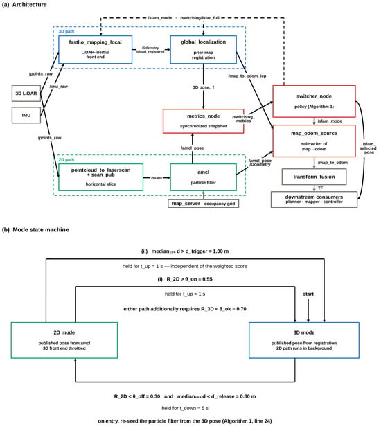
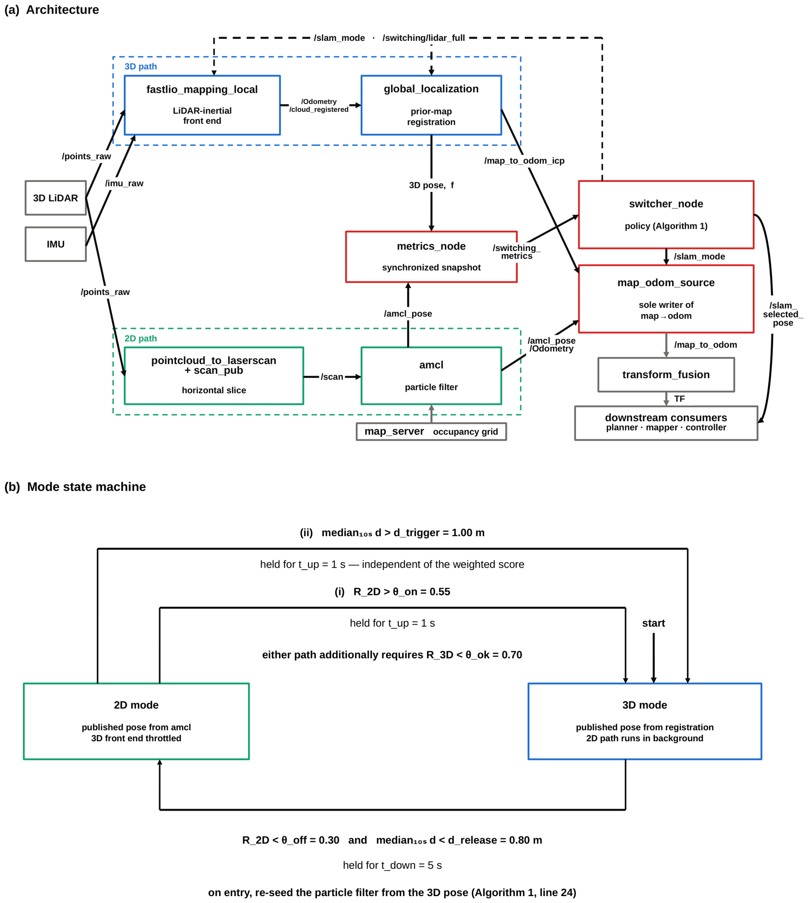
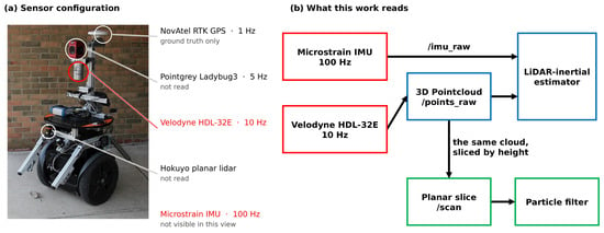
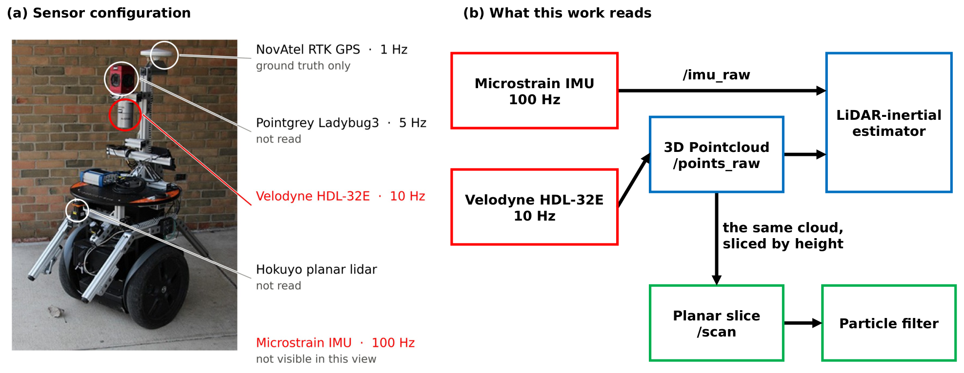
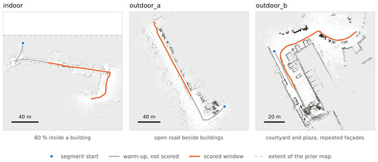
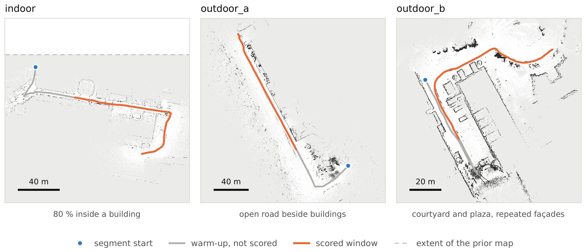
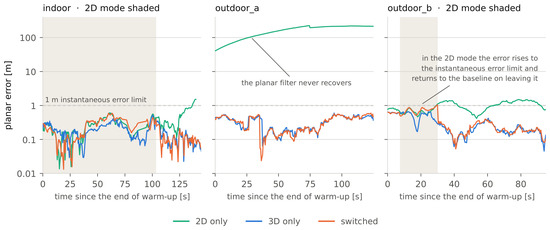
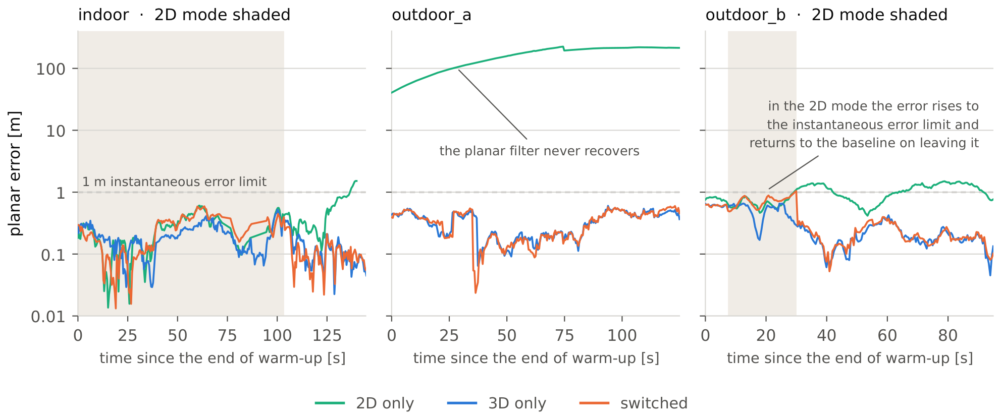
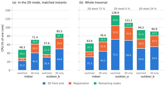
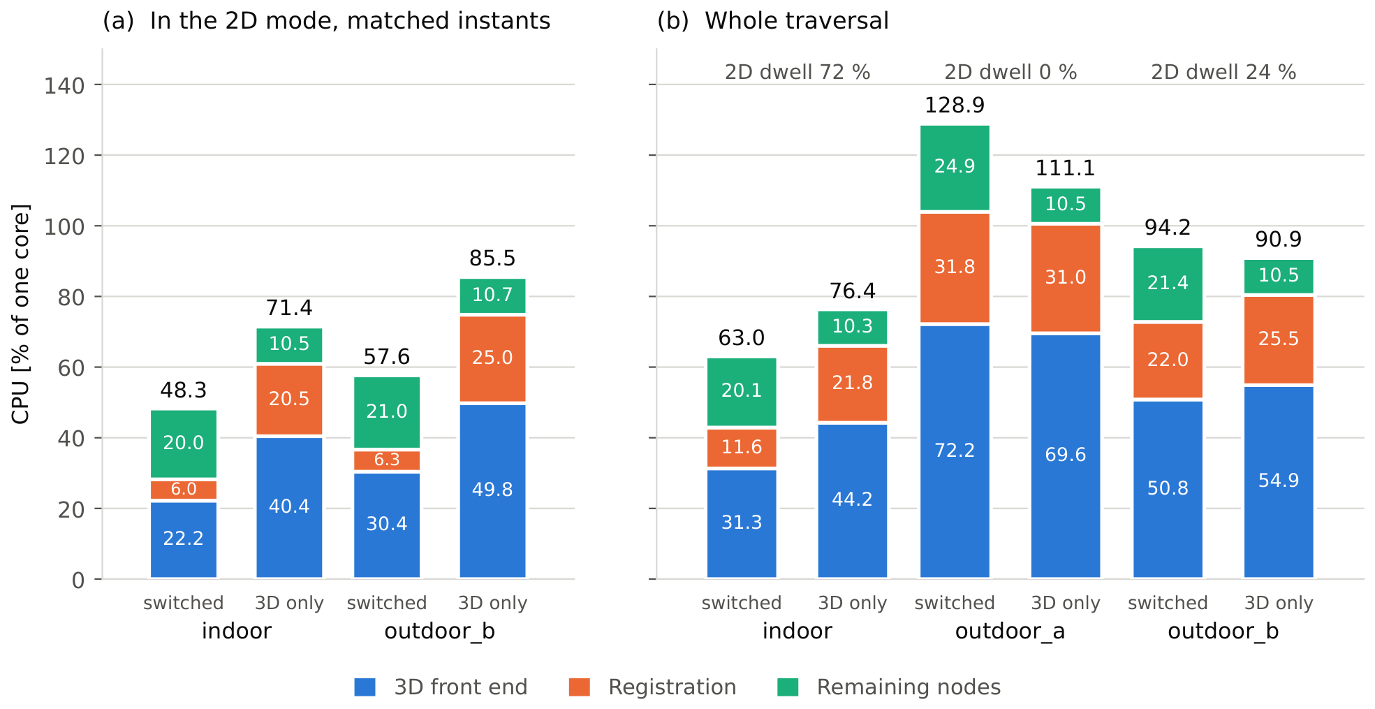
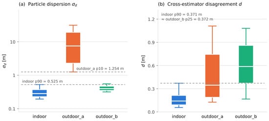
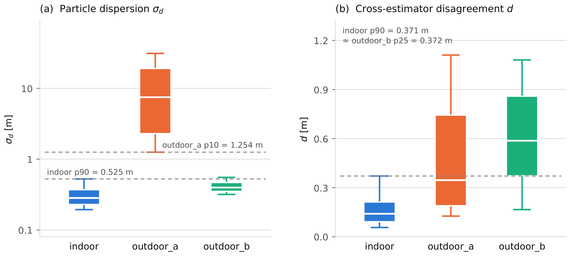

Disclaimer/Publisher’s Note: The statements, opinions and data contained in all publications are solely those of the individual author(s) and contributor(s) and not of MDPI and/or the editor(s). MDPI and/or the editor(s) disclaim responsibility for any injury to people or property resulting from any ideas, methods, instructions or products referred to in the content. |
© 2026 by the authors. Licensee MDPI, Basel, Switzerland. This article is an open access article distributed under the terms and conditions of the Creative Commons Attribution (CC BY) license.