


Abstract
Sequential recommendation must infer evolving preferences from interaction histories that are sparse, temporally irregular, and heterogeneous in relevance. Existing diffusion-based recommenders improve representation generation and recovery, yet their perturbation strength is typically governed by the diffusion step and does not explicitly reflect the temporal state of each historical interaction. We propose ISDSRec, an interaction-specific diffusion scheduling framework that uses local interaction gaps to represent behavioral rhythm and global recency to derive a position-specific temporal prior. This prior modulates a shared base diffusion schedule so that interactions at the same diffusion step can receive different effective noise intensities. A diffusion-step- and recency-conditioned bidirectional Transformer denoiser predicts the injected Gaussian noise, from which clean interaction representations are recovered analytically. The same temporal prior is reused as a recency bias in long-term attention, while behavioral statistics regulate long- and short-term preference fusion. Item textual metadata are encoded offline by a frozen GTE-Qwen2-7B-instruct model and adaptively fused with trainable ID embeddings. Experiments on three Amazon Review categories and MovieLens-1M show that ISDSRec achieves the highest mean performance across all 16 dataset–metric settings at K = 5 and K = 10, with relative gains of 6.17–8.55% over the strongest competing baselines. Controlled analyses examine the contributions of semantic representation, diffusion-based recovery, interaction-specific scheduling, and preference reconstruction. NDCG@10 improvements over shuffled-recency, reversed-recency, position-based scheduling, Clean-Input Transformer, and Temporal-GTE SASRec controls reach Holm-adjusted significance across all four datasets. NDCG@10 improvements over Noise-Matched Uniform and the Heteroscedastic Gaussian DAE reach Holm-adjusted significance only on MovieLens-1M. Stratified, stochastic-inference, and efficiency analyses further characterize the model under different temporal, behavioral, and practical inference conditions.
1. Introduction
The rapid growth of e-commerce, video platforms, and online content services has generated large volumes of temporally ordered user-item interactions. Sequential recommendation predicts a user’s next interaction from this chronological history [1,2,3], but the relevance of historical behaviors is not temporally uniform. Interactions may occur at irregular intervals, span very different time horizons, and contribute unequally to the current preference state. Effective next-item prediction therefore requires sequence modeling with explicit treatment of temporal heterogeneity in dynamic interaction data.
Deep sequential recommendation has progressed from recurrent neural networks [4] and convolutional neural networks [5] to Transformer-based self-attention architectures [6,7], with subsequent extensions based on graph neural networks [8]. These models improve the representation of behavioral dependencies, but many still rely primarily on item IDs and interaction order. Lower-activity users and lower-frequency items provide less collaborative evidence for representation learning, which can reduce representation quality under these conditions.
Pretrained language models and large language models can supply content semantics from item titles, categories, and descriptions [9,10]. These representations complement collaborative ID embeddings, especially when interaction evidence is limited. However, a general semantic embedding space is not automatically aligned with the recommendation space, and fixed addition or concatenation cannot adjust the semantic–collaborative balance across items and latent dimensions.
Semantic enrichment addresses item-representation sparsity, but it does not resolve how diffusion should treat historical interactions that occupy different temporal states. Existing time-aware recommenders usually inject time into representations, recurrent updates, or attention [11], whereas diffusion-based sequential recommenders mainly differ in diffusion targets, conditioning information, and recovery procedures [12,13]. Their perturbation schedules remain primarily functions of the diffusion step. Consequently, two historical interactions with very different recency can receive similar perturbation strength, limiting position-level control of representation corruption and recovery.
Motivated by this gap, we propose ISDSRec, an interaction-specific diffusion scheduling framework for sequential recommendation. Its central mechanism converts a shared diffusion-step schedule into position-dependent effective noise levels by using global interaction recency as an explicit temporal control signal. Local interaction gaps separately characterize behavioral rhythm in the input states, while a diffusion-step- and recency-conditioned bidirectional Transformer denoiser predicts the injected Gaussian noise and supports analytical recovery of the clean interaction representations. The same recency-derived temporal prior is further reused to coordinate long-term preference aggregation with short-term intent, providing consistent temporal semantics from representation recovery to preference reconstruction. As a complementary component, frozen GTE-Qwen2-7B-instruct embeddings are generated offline and adaptively fused with trainable item ID embeddings through dimension-wise gating.
The following four research questions guide the evaluation:
- RQ1: Does interaction-specific diffusion scheduling, driven by heterogeneous temporal conditions, improve next-item recommendation compared with shared or uniform diffusion schedules?
- RQ2: Do LLM-derived semantic representations and dimension-wise semantic–collaborative fusion provide complementary gains for next-item recommendation, particularly when collaborative evidence is limited?
- RQ3: How do temporal weighting, adaptive long- and short-term preference fusion, and shared temporal-prior coordination contribute to preference reconstruction and next-item prediction?
- RQ4: How stable is ISDSRec across temporal, user-activity, and item-popularity strata and parameter settings, and what are its stochastic-inference and practical-efficiency characteristics?
The contributions are:
- We introduce interaction-specific diffusion scheduling for sequential recommendation. A recency-derived temporal prior modulates a shared diffusion-step schedule, assigning different effective perturbation strengths to historical interactions at the same diffusion step. Controlled comparisons with shuffled-recency, reversed-recency, and position-based schedules show significant NDCG@10 improvements after Holm correction across all four datasets. The comparison with Noise-Matched Uniform reaches Holm-adjusted significance only on MovieLens-1M.
- We construct a complementary LLM-derived semantic–collaborative item representation. A frozen GTE-Qwen2-7B-instruct model encodes item text offline, and a dimension-wise gate adaptively integrates semantic representations with trainable ID embeddings without requiring online LLM inference.
- We develop temporally coordinated preference reconstruction. The recency-derived temporal prior used for interaction-specific diffusion is reused as a bias in long-term preference aggregation, while observable behavioral statistics regulate the balance between long-term preference and short-term intent. This links temporal reliability across representation recovery and final user-state construction.
- We evaluate ISDSRec on four benchmark datasets, comprising three Amazon product categories and MovieLens-1M, against nine representative baselines. The evaluation combines repeated-run statistical analysis, mechanism-matched controls, temporal-prior role isolation, a focused semantic-by-scheduling factorial analysis, stratified evaluation, parameter sensitivity, test-time Gaussian-noise analysis, and measured practical efficiency.
The experiments cover e-commerce and movie recommendation settings with item-level textual metadata.
2. Related Work
2.1. Deep Sequential Recommendation
Early sequential recommenders commonly used Markov chains and matrix factorization to model user preferences and item transitions. FPMC combines matrix factorization with a first-order Markov chain to represent long-term user preferences and transitions between adjacent items within a single framework [14].
GRU4Rec recursively updates a session state with gated recurrent units and uses the hidden state to represent the user’s current interest [4]. Caser arranges a user’s interaction sequence as a two-dimensional embedding matrix, applies horizontal convolutions to extract local sequential patterns of different lengths, and uses vertical convolutions to aggregate features across positions [5]. SASRec employs unidirectional self-attention with a causal mask to aggregate historical interactions and preserves order through positional embeddings [6]. BERT4Rec adopts a bidirectional Transformer and a masked-item prediction task to learn context-dependent representations by recovering masked items [7]. SR-GNN represents session items as nodes and adjacent interactions as directed edges, and propagates node states through a gated graph neural network [8].
2.2. Time-Aware Sequential Recommendation
A user interaction sequence contains both behavioral order and irregular time intervals. TiSASRec adds time-interval relation embeddings to the self-attention mechanism of SASRec so that attention jointly accounts for item relevance and temporal distance [11]. MEANTIME encodes absolute time, relative time, and sequential position and combines these temporal views through multi-channel attention [15]. MTAM updates recent states with a time-aware recurrent unit and aggregates long-term history through a multi-hop memory network [16]. Deja Vu jointly models event content and occurrence time with contextualized temporal attention to compute time-dependent weights for historical interactions [17].
Temporal information is typically injected into input representations, state updates, or attention calculations. A local gap measures the temporal distance between consecutive behaviors, whereas global recency indicates the temporal position of a historical interaction relative to the end of the observed sequence. The two variables therefore characterize behavioral rhythm and historical position, respectively.
2.3. Recommendation Enhanced by Pretrained Language Models and LLMs
Pretrained language models and LLMs can encode item titles, categories, and descriptions as semantic representations and combine them with collaborative representations learned from interactions. UniSRec builds transferable sequence representations through a pretrained text encoder, parametric whitening, a mixture-of-experts adaptor, and cross-domain contrastive learning [9]. Recformer organizes textual item attributes as language sequences and jointly learns item and user-sequence representations through language-model pretraining and sequential-recommendation fine-tuning [10].
LLM-ESR constructs a semantic view from LLM embeddings and combines it with retrieval-enhanced self-distillation to learn representations for long-tail users and items [18]. LLMEmb injects collaborative information into LLM-generated item embeddings through supervised contrastive fine-tuning and recommendation-oriented adaptation [19]. Methods in this category generally generate textual semantic representations offline and rely on a sequential recommender for user modeling and next-item prediction.
Another line of work reformulates recommendation as natural-language generation or generative retrieval. P5 uses a text-to-text framework to represent multiple recommendation tasks in a unified form [20]. TALLRec aligns an LLM with recommendation objectives through parameter-efficient instruction tuning [21]. TIGER maps items to discrete semantic IDs and predicts the target identifier with a generative retrieval model [22].
2.4. Diffusion Models for Sequential Recommendation
Diffusion models gradually add noise to a data representation through a forward process and learn a reverse process to recover the original representation or generate a target sample [23]. In sequential recommendation, existing studies mainly differ in the diffusion target, conditioning information, and recovery procedure.
DiffuRec treats the target-item embedding as the diffusion variable, adds Gaussian noise in a continuous representation space, and reconstructs the target representation conditioned on the user’s historical sequence [12]. DreamRec formulates next-item prediction as guided diffusion generation and progressively generates the target-item representation from historical behavioral conditions [13]. DimeRec further incorporates multiple user-interest representations as conditioning signals to guide diffusion-based recommendation [24]. Developed more recently, ADRec applies diffusion independently to interaction representations at different sequence positions and combines token-level diffusion with autoregressive sequence modeling and staged optimization to alleviate representation collapse during diffusion training [25].
Diffusion-based sequential recommenders therefore differ in diffusion objects, conditioning representations, and recovery strategies. Existing methods typically diffuse a target item, an aggregated user-interest representation, or position-level interaction representations, while the noise schedule remains governed mainly by the diffusion step. ADRec extends diffusion to different interaction positions. Its perturbation process lacks explicit control from the temporal state of each historical interaction. This distinction motivates interaction-specific diffusion scheduling, in which a shared diffusion stage is converted into heterogeneous position-level perturbation strengths according to temporal reliability.
2.5. Multi-Interest and Dynamic Preference Modeling
A user’s history often contains multiple interest directions and preference changes over different time scales. Existing research has considered multi-interest extraction, multi-granularity interest representations, and long- and short-term preference fusion. For multi-interest extraction, MIND aggregates historical behaviors into multiple interest capsules through dynamic routing and selects the interest most relevant to a candidate item [26]. ComiRec further develops two multi-interest extraction architectures based on self-attention and dynamic routing and combines the resulting interests through controllable aggregation [27]. PoMRec addresses the different optimization objectives of interest extractors and aggregators by introducing task-specific prompts, allowing interaction representations to adapt separately to extraction and aggregation. It also uses mean and variance embeddings to characterize the center and dispersion of an interest distribution [28]. MGUI models user interests at individual, group, and global levels [29]. For long- and short-term preference modeling, SHAN uses a two-layer hierarchical attention network that first extracts long-term preference from historical interactions and then combines it with recent behavior to form the final user representation [30].
ALSTP introduces time-aware and content-aware controllers into recurrent state updates and integrates long- and short-term preferences through attention [31]. DMAN divides a long sequence into multiple subsequences, stores long-term interests in dynamic memory blocks, and combines them with recent behavior for recommendation [32]. TLSRec models global and local preferences with hierarchical self-attention and regulates the two representations through a neural temporal gate [33]. These studies establish the value of dynamic preference modeling, but temporal weighting in preference aggregation is usually treated separately from diffusion perturbation. Within diffusion-based sequential recommendation, limited attention has been paid to using a shared temporal condition both to regulate interaction-level perturbation strength and to coordinate subsequent preference reconstruction. This motivates the temporal-prior coordination adopted in the proposed framework.
3. Methodology
3.1. Problem Formulation and Framework Overview
3.1.1. Problem Formulation
Let and denote the sets of users and items, respectively. For each user , the chronologically ordered interaction sequence is defined as
where is the item interacted with at sequence position , is the corresponding timestamp, and is the total number of interactions of user . This formulation follows the standard sequential recommendation setting, in which future user behavior is predicted from temporally ordered historical interactions [1,3,6].
For an instance whose prediction target is the interaction at position , only the preceding interactions are observable. The historical prefix and prediction target are respectively written as
where the prefix length is .
Each item is associated with textual metadata consisting of its title, category, and description.
Next-item prediction is formulated as learning a parameterized recommender that estimates the matching score between the current user preference state and each candidate item [5,6,7,9]. During evaluation, candidate items are ranked by these scores, and the highest-ranked item is treated as the predicted next interaction.
To preserve causality, the target item , its timestamp, and all subsequent interactions are excluded from every downstream stage, including sequence encoding, temporal-variable construction, behavioral-statistics computation, and preference reconstruction.
3.1.2. Framework Overview
ISDSRec comprises four modeling stages followed by candidate scoring for final recommendation (Figure 1): semantic–collaborative item representation, temporal input construction, interaction-specific diffusion and direct recovery, and dynamic preference reconstruction. Its central mechanism modulates a shared diffusion schedule according to each historical interaction’s recency [23].
Figure 1.
Overview of the proposed ISDSRec framework.
Following recent decoder-only LLM embedding approaches [34], frozen GTE-Qwen2-7B-instruct embeddings provide offline item semantics. The Qwen2-7B backbone of the semantic encoder is based on Transformer self-attention [35], while its model-specific configuration and inference procedure follow the official model repository [36]. Local gaps encode behavioral rhythm, while global recency supplies a shared prior for noise scheduling, denoiser conditioning, and long-term attention [11,15,16,17].
Training samples one diffusion step per instance. A bidirectional Transformer predicts the position-specific injected noise, and clean states are recovered analytically. Behavioral statistics then control long- and short-term preference fusion.
Inference uses a validation-selected operating point fixed for each dataset: zero uses clean states directly, and a nonzero value applies one perturbation and one denoising pass. Neither mode performs iterative reverse diffusion.
3.2. LLM-Derived Semantic–Collaborative Item Representation
3.2.1. Offline LLM-Derived Item Semantic Encoding
Each item is associated with textual metadata:
These fields are concatenated in a fixed order with explicit field identifiers to construct the textual input . Missing fields are replaced by a shared placeholder while the field order is retained. If exceeds the maximum input length , measured in encoder tokens, the title and category are preserved and the description is truncated to the remaining token budget.
We use the frozen Alibaba-NLP/gte-Qwen2-7B-instruct model as the semantic encoder. It follows the recent paradigm of using decoder-only LLMs as general-purpose text encoders [34]. The official model repository identifies Qwen2-7B as its backbone [36], whose architecture is based on Transformer self-attention [35]. Following the model’s official configuration and inference procedure, last-token pooling is applied: the hidden state of the final valid non-padding token is taken as the item-level semantic embedding and subsequently L2-normalized to obtain [36].
Because the LLM embedding dimension differs from the recommendation latent dimension , a trainable projection layer maps the normalized embedding into the recommendation space:
where denotes layer normalization [37]. All item-level LLM embeddings are generated once and cached before recommender training. The semantic encoder remains frozen, whereas the projection and layer-normalization parameters are jointly optimized with the recommendation objective. The same encoding and projection pipeline is used for all datasets, and the resulting serves as the task-adapted semantic representation of item . For the adopted GTE-Qwen2-7B-instruct encoder, the cached semantic vector has 3584 dimensions, and the recommendation latent dimension is 128. The trainable projection is therefore implemented as Linear(3584, 128) followed by LayerNorm(128).
3.2.2. Gated Semantic–Collaborative Fusion
The semantic representation captures content-level information, whereas the trainable ID embedding retains collaborative signals. Because their relative contributions may vary across items and dimensions, ISDSRec performs dimension-wise gated fusion based on their concatenated representation:
where denotes vector concatenation, and is the sigmoid activation. Each dimension of the gate vector independently controls the relative contribution of the collaborative and semantic representations in the corresponding latent dimension. With d = 128, the concatenated semantic-ID input is 256-dimensional, and the gate is implemented as Linear(256, 128) followed by an element-wise sigmoid.
The semantic–collaborative representation of item is defined as
where ⊙ denotes element-wise multiplication. A gate value close to 1 retains more collaborative information from the ID embedding in that dimension, whereas a value close to 0 assigns greater weight to the LLM semantic representation. All gate dimensions are learned end-to-end with the recommendation objective, which allows the semantic–collaborative balance to vary across both items and latent dimensions. Historical and candidate items use the same semantic encoder, projection layer, ID embedding table, and gated-fusion parameters, placing both sides of the scoring function in a common recommendation space [9,10,18,19].
3.3. Temporal Condition Modeling and Diffusion-Input Construction
Drawing on interval-aware sequential recommendation, ISDSRec separately encodes local interaction gaps and global recency distances to capture complementary temporal signals [11,15,16,17,33]. To avoid ambiguity between positions before and after truncation, we distinguish two indices: denotes an original position in the complete observable prefix, and denotes a valid position in the truncated model input. All temporal variables are first computed over the complete observable prefix, after which the retained positions are selected through a position mapping.
3.3.1. Local Interaction-Gap Encoding
For prediction target position , the complete observable prefix has length , and its original positions are indexed by . For , the local interaction gap is defined as
where represents one day in the timestamp unit of the dataset. A value of zero indicates that two interactions occurred on the same day. The true first interaction has no preceding timestamp. The missing interval denotes a structural sequence boundary and does not represent an observed zero-day gap.
To reduce the effect of highly skewed temporal gaps, valid intervals are log-transformed and standardized using statistics computed from valid interaction pairs in the training set:
where and are the mean and standard deviation of the log-transformed intervals in the training set, respectively, and is a small constant for numerical stability. Transforming and normalizing irregular intervals reduces instability caused by heterogeneous temporal scales. A two-layer multilayer perceptron (MLP) then maps the standardized gap into the -dimensional latent space:
where is the GELU activation, and , , , and are trainable parameters. The gap encoder uses the fixed architecture consisting of Linear(1, 64), GELU, and Lin-ear(64, 128), with no dropout in this branch. Unlike methods that discretize temporal gaps into predefined bins [11], this continuous mapping converts temporal distance into a dense vector aligned with the item-representation dimension without introducing manual bin boundaries. A learnable boundary embedding is used for the true first interaction:
The boundary embedding marks only the true beginning of the observable sequence and distinguishes a missing predecessor from an observed zero-day interval. For histories longer than the maximum sequence length, only the most recent interactions are retained and reindexed chronologically. The boundary embedding is a trainable 128-dimensional vector.
Local gaps are therefore computed before truncation. When the first retained interaction is not the true first interaction of the observable prefix, its gap is still computed from the immediately preceding original timestamp. The model input excludes that preceding interaction. The boundary embedding is used only when the retained position corresponds to the true sequence boundary.
3.3.2. Global Interaction-Recency Modeling
Previous time-aware sequential recommendation studies show that the influence of historical behavior on current preference often changes with temporal distance. Modeling only adjacent interaction gaps may therefore be insufficient to describe the temporal decay of long-term preference [15,16,17,33]. ISDSRec uses the final interaction in the complete observable prefix as a common reference and constructs a position-level global recency signal. The observation endpoint is defined as
This reference point is the most recent historical interaction observable when predicting position . It does not use the target-interaction timestamp , thereby preserving causality in temporal-variable construction. For original position , the global recency distance is
Here, one day is used as the timestamp unit. The final observable interaction has zero recency by definition.
A smaller recency distance therefore indicates an interaction closer to the current observation endpoint, whereas a larger value indicates an earlier interaction. Unlike sequential positions, which encode only behavioral order, this temporal distance explicitly represents the irregular elapsed time between interactions [15,16,17].
Truncation selects positions without changing their reference timestamp or temporal relationships. Subsequent position-level computations use retained index k.
3.3.3. Diffusion-Input Construction
Because a local interaction gap does not uniquely identify sequence order, a learnable absolute positional embedding is introduced for each valid position. The positional embedding table is optimized jointly with the other model parameters. The pre-diffusion interaction state is defined as
where LN(·) denotes layer normalization [37]. The item representation supplies semantic and collaborative information, the gap embedding supplies local timing information, and the absolute position identifies the interaction order after truncation. Valid interaction states are stacked chronologically. In the experiments, the learnable absolute positional-embedding table has size 50 × 128, matching the maximum retained history length and latent dimension.
For mini-batch computation, sequences shorter than the maximum sequence length are left-padded. A validity mask distinguishes retained interactions from padding positions.
The validity mask is applied throughout subsequent computation. Position indices represent the relative order of valid interactions and remain independent of physical columns after left padding. Padding positions receive no valid positional representation and are excluded from self-attention, perturbation, recovery, preference aggregation, and loss computation [6,7,11].
3.4. Interaction-Specific Diffusion Scheduling and Direct Recovery
Equation (13) yields a clean interaction state for each retained position. ISDSRec derives a recency-based temporal condition that modifies the shared diffusion schedule at the interaction level and reflects the temporal separation between earlier and more recent behaviors. Recent interactions retain more signal, while earlier interactions receive stronger perturbation and must rely more on sequence context during recovery.
3.4.1. Recency-Based Temporal Prior
Global interaction-recency distance measures the temporal separation between the historical interaction at retained position and the observation endpoint. Raw recency distances are typically right-skewed and can vary substantially across datasets. Before diffusion scheduling, they are therefore log-compressed and normalized:
where is the standard deviation of the log-transformed recency distances computed from the training data, and is a small constant for numerical stability. Mean centering is not applied so that the normalized distances remain non-negative and preserve the temporal order of historical interactions.
The interaction-specific temporal condition is defined as
where is a decay coefficient selected on the validation set. Previous studies have shown that the contribution of historical interactions varies with temporal distance [16,17,31]. ISDSRec applies an exponential transformation to map each non-negative recency distance to a bounded temporal condition. A larger corresponds to a more recent interaction and retains more of the original signal during diffusion. A smaller corresponds to an earlier interaction and receives stronger perturbation. The same prior modulates diffusion scheduling in Section 3.4.2, conditions the denoiser in Section 3.4.4, and biases long-term attention in Section 3.5.1, coordinating one deterministic recency signal across the three stages. The recency prior is implemented as a deterministic exponential transformation, with no neural encoder. Its decay coefficient is selected on the validation set and is not updated by backpropagation.
3.4.2. Recency-Modulated Interaction-Specific Noise Scheduling
Let denote a predefined linear base noise schedule, following the progressive corruption mechanism of classical diffusion models [23]:
where and are the minimum and maximum base noise rates, respectively, and is the total number of diffusion steps. Existing diffusion-based sequential recommenders commonly apply a predetermined schedule to the entire sequence according to diffusion step [12,24]. To further distinguish the temporal reliability of historical interactions, ISDSRec modulates the base noise rate with the position-level temporal prior :
where controls the extent to which the temporal condition modulates noise strength. For the most recent interaction, , and the noise rate reduces to the base value . For an earlier interaction, , and the noise rate increases as recency decreases. Different positions within the same diffusion step therefore receive different effective perturbation strengths.
To keep the noise rate at every position within a valid range, the modulated value is capped at :
This clipping ensures , so that the corresponding signal-retention coefficient remains positive. The one-step signal-retention coefficient and its cumulative form for position at diffusion step are defined as
The cumulative signal-retention coefficient follows the standard forward-distribution construction from step-wise noise rates [23]. In ISDSRec, however, depends jointly on the diffusion step , user , and interaction position . All positions within an instance share the same diffusion step. Individual historical interactions retain different signal amounts according to recency.
To limit tuning complexity, the base-schedule parameters , , and are fixed in all experiments. The temporal decay coefficient , temporal modulation strength , and diffusion-loss weight are selected on the validation set. After training, the inference operating point is determined separately according to validation NDCG@10. The clipping upper bound is fixed to in all experiments as a fixed numerical safeguard and is excluded from hyperparameter tuning.
3.4.3. Interaction-Specific Forward Diffusion
During training, one diffusion step is sampled independently and uniformly from the available diffusion steps for each prediction instance.
All valid positions within an instance share the sampled step , maintaining a consistent sequence-level noise stage. Each position nevertheless uses its own cumulative signal-retention coefficient , so the effective perturbation strength is still determined by the interaction-specific schedule in Section 3.4.2. Random diffusion-step sampling trains the model to recover representations under multiple noise levels [38].
Under the closed-form reparameterization of diffusion models, a noisy state at any diffusion step can be sampled directly from the unperturbed state without sequentially generating the intermediate states [38,39]:
where
Equation (20) combines the original interaction state with standard Gaussian noise. The position-specific cumulative signal-retention coefficient controls the retained signal and injected noise, so recent and earlier interactions can receive different noisy states even when they share the same diffusion step.
The validity mask excludes padded positions from forward perturbation, so only valid noisy interaction states are passed to the diffusion-step- and recency-conditioned bidirectional Transformer denoiser in Section 3.4.4.
3.4.4. Diffusion-Step- and Recency-Conditioned Transformer Denoising
Given the noisy interaction matrix , ISDSRec uses a shared epsilon-prediction denoiser to estimate the injected Gaussian noise. Because diffusion steps correspond to different noise levels, an explicit step embedding is introduced:
The diffusion-step index is encoded by a trainable lookup so that the same denoiser can operate across all sampled noise levels [23,38]. The lookup returns a 128-dimensional vector. With T = 100, the implementation uses Embedding(101, 128), where index 0 is reserved for convenience and training samples steps from 1 to 100.
For each valid position , the denoiser input combines the noisy interaction state, diffusion-step embedding, and position-level temporal prior:
The step embedding provides all positions in an instance with shared information about the noise stage, whereas the projected temporal prior preserves differences in temporal reliability across positions. Consequently, even when all positions share diffusion step , the denoiser can identify their different forward-perturbation trajectories. The scalar recency prior is projected by a trainable Linear(1, 128) layer and added to the denoiser input, providing a conditioning pathway distinct from its schedule-modulation role in Equation (17).
A two-layer Pre-LayerNorm bidirectional Transformer encoder then models the full noisy interaction sequence in context:
Bidirectional attention allows each valid position to use both preceding and subsequent interactions within the history to recover its perturbed representation, consistent with conditional denoising over complete historical context in diffusion-based sequential recommendation [24,40,41]. The attention operates only on the observable historical prefix and includes neither the target item nor future interactions. This restriction satisfies the causal constraint in Section 3.1.1. Padded positions are excluded from attention by . The denoiser uses model dimension 128, four self-attention heads (32 dimensions per head), feed-forward dimension 512, GELU activation, and dropout 0.1. Only the padding mask is applied. No causal triangular mask is used because all positions belong to the observable historical prefix.
For each valid position , the Transformer output is passed through a trainable Linear(128, 128) noise-prediction head to estimate the injected noise:
Using the interaction-specific cumulative signal-retention coefficient from Section 3.4.3, the clean interaction representation is then recovered analytically from the predicted noise:
This recovery expression follows directly from the closed-form reparameterization of forward diffusion [23,38]. Because is position-specific, historical interactions use their own signal-retention coefficients for recovery even when they share a diffusion step.
The recovered interaction states are stacked chronologically and supplied to the dynamic preference reconstruction module in Section 3.5. Padded positions are excluded from denoising, recovery, and subsequent aggregation.
To prevent longer sequences from accumulating a larger loss during optimization, the denoising loss is normalized by the total number of valid latent dimensions in the mini-batch:
where denotes the current mini-batch. This normalization gives equal weight to every valid latent dimension and keeps the loss scale invariant to the distribution of sequence lengths within a mini-batch.
Because diffusion steps are sampled uniformly from during training, the same denoiser is jointly optimized across multiple noise levels without a separate network for each step. Equation (26) analytically recovers and does not explicitly generate intermediate reverse states. Recent studies have likewise explored skip-step sampling or one-step denoising to reduce the iterative inference cost of diffusion recommenders [40,41,42]. Unlike approaches that compress a generative sampling trajectory, ISDSRec treats diffusion as multi-noise-level representation recovery and directly obtains interaction representations for preference reconstruction at a selected operating point.
3.5. Temporally Coordinated Dynamic Preference Reconstruction
The denoising stage returns one recovered representation for each valid historical interaction, whereas candidate scoring requires a single user vector. ISDSRec forms this vector from two complementary views of the recovered history. A recency-biased additive attention layer aggregates long-term evidence, the final recovered state represents short-term intent, and behavioral statistics determine how the two components are fused.
3.5.1. Long- and Short-Term Preference Extraction
After recovering the interaction representations, ISDSRec extracts long-term and short-term preferences from the complete truncated valid history and the most recent interaction, respectively. Recent studies also indicate that relatively stable preferences in the complete history and dynamic intent reflected by recent behavior are complementary and should be modeled through separate branches [43,44]. Let denote the effective truncated-sequence length of user , and let be the recovered interaction representation at valid position , where .
Because historical interactions contribute differently to the current prediction, the long-term branch applies single-layer additive attention to the recovered sequence and introduces the shared temporal prior defined in Section 3.4.1 as a recency bias:
where the attention parameters are trainable. The additive-attention hidden dimension is fixed to 128, matching the recommendation latent dimension.
The trainable scalar controls the influence of the temporal prior on long-term attention. The position-specific prior directly biases each attention logit according to recency, so attention depends on content relevance and temporal position. Single-layer additive attention over the complete history is a common strategy for extracting long-term preference in recent long- and short-term preference models [43,44].
The short-term branch directly uses the interaction representation at the final valid position of the recovered sequence:
The final valid recovered state is used directly as the short-term representation because it is temporally closest to the prediction point. The long-term branch aggregates evidence from the complete valid history, while the short-term branch preserves the most recent recovered state without introducing another trainable network. Both branches use only observable history and exclude the target item, target timestamp, and subsequent interactions.
3.5.2. User Behavioral-Statistics Encoding
All sequence-level statistics are computed over the valid truncated positions . The activity span covers only the retained interaction sequence, and the mean local gap includes only temporal differences between adjacent retained positions and . The truncation-boundary gap used in Section 3.3.1 to construct the input at the first retained position is excluded from the mean local gap, preventing interactions outside the retained sequence from being introduced again into user-level statistics.
Sequence length, temporal span, and interaction rhythm characterize a user’s behavioral history and provide additional context for personalized long- and short-term preference fusion [15,16,29,33]. ISDSRec therefore constructs the behavioral-statistics vector
where the vector contains effective sequence length, activity span, mean local interaction gap, an interval-validity indicator, and the mean and dispersion of the shared temporal prior. The activity span is the elapsed time between the first and final retained interactions, and the mean local gap averages adjacent retained interactions when at least two valid interactions are available. When only one valid interaction is present, the mean gap is assigned a zero placeholder and the validity indicator marks it as unavailable, preventing structural missingness from being interpreted as an observed zero-day gap. Sequence length and activity span are log-transformed to reduce skew.
The mean and standard deviation of the shared temporal prior over valid positions are defined as follows:
These quantities describe the mean and dispersion of recency over valid positions. Dispersion is zero for a single-position history.
Before the behavioral encoding layer, continuous statistics are standardized using statistics computed exclusively from the training set, while the binary interval-validity indicator remains unchanged.
A single fully connected behavioral-statistics encoder then produces the user-level statistics representation:
where and are trainable parameters, and is the GELU activation. The resulting vector is the direct input to the scalar long- and short-term fusion gate in Section 3.5.3. The input vector contains six statistics, and the encoder is implemented as Linear(6, 128) followed by GELU.
3.5.3. Adaptive Long- and Short-Term Preference Fusion
The relative contributions of long- and short-term preferences to next-item prediction may vary with a user’s history length, interaction rhythm, and temporal distribution. ISDSRec therefore estimates a user-specific scalar gate from the behavioral-statistics representation obtained in Section 3.5.2. Dynamic fusion of long- and short-term preferences has also been used to construct user representations in time-aware sequential recommendation [31,33]:
where and are trainable parameters, and is the sigmoid function. The fusion gate controls the relative contributions of the two preference components. A larger makes the final representation rely more heavily on the long-term preference aggregated from the complete valid history, whereas a smaller places greater emphasis on the short-term intent reflected by the most recent recovered interaction.
A scalar gate is used because and are both constructed from recovered interaction states, reside in the same latent space, and describe user preference at the current prediction time. The scalar gate provides a user-level balance between two homogeneous preference components. By contrast, the dimension-wise gate in Section 3.2.2 integrates semantic and ID representations with different origins and properties and must regulate the two information sources separately across latent dimensions.
3.6. Next-Item Prediction and Optimization
3.6.1. Candidate Scoring and Joint Optimization
Given the dynamic user preference representation and the semantic–collaborative representation of a candidate item, next-item relevance is computed by their inner product, a standard matching function in sequential recommendation [6,9,12].
Historical and candidate items share the item representation function defined in Section 3.2, placing user preferences and candidate representations in the same latent space. For each training instance, the candidate set contains one ground-truth next item and 100 negative items sampled uniformly without replacement from the item catalog after excluding the ground-truth target and items appearing in that instance’s observable prefix. Negative items are re-sampled at each epoch. Interactions occurring after the current target, including later training events and the held-out validation and test interactions, are not used to filter the training negative pool.
A sampled-candidate softmax cross-entropy loss ranks the target against its sampled negatives [6,9,22]:
The denominator covers only the sampled candidates, without full-catalog normalization or a negative-sampling correction.
Recommendation and noise-prediction objectives are jointly optimized [12,24]:
The validation-selected diffusion-loss weight balances the two objectives. At zero, training uses only the recommendation loss. Otherwise, noise-prediction gradients also reach upstream trainable representations because clean states are not detached. The frozen GTE encoder and cached embeddings remain outside gradient computation.
3.6.2. Training Procedure
Training first retrieves cached semantics and constructs masked interaction states from the observable prefix. For each instance, it samples a diffusion step, applies recency-modulated Gaussian noise, predicts that noise, and analytically recovers the clean states.
Preference reconstruction aggregates the recovered states. Target and negative-item scores then define the recommendation loss, optimized jointly with the denoising loss in Equation (37).
Trainable components include semantic projection and fusion, ID and positional embeddings, gap encoding, step and recency conditioning, the Transformer and noise head, long-term attention, and the behavioral-statistics gate. The GTE encoder and cached vectors remain fixed.
The recency prior is deterministic. Its decay, noise modulation, diffusion-loss weight, and inference operating point are validation-selected. The base schedule and clipping bound are fixed.
3.6.3. Inference and Top-K Recommendation
The inference operating point is selected by validation NDCG@10 and fixed for the dataset:
The selected value is then fixed for all test instances in that dataset. The validation search set is in {0, 20, 40, 50, 60, 80}; denotes clean-input inference.
At zero, clean interaction states enter preference reconstruction directly. At a nonzero step, Equation (20) generates one noisy input, followed by one denoiser call and analytical recovery via Equation (26). No iterative reverse diffusion is used.
The unified interaction-state matrix used for dynamic preference reconstruction is defined as:
Section 3.5 aggregates these states into a user vector. Inner-product scores then rank candidate items for Top-K recommendation.
3.6.4. Complexity Analysis
The frozen LLM encoder is used only during offline preprocessing, and the resulting item semantic embeddings are cached before recommender training. Its computational cost is therefore excluded from the online inference complexity.
Let denote the effective sequence length, the latent dimension, and the number of candidate items. The dominant computation is the two-layer diffusion-step- and recency-conditioned bidirectional Transformer denoiser, for which a single forward pass requires approximately . During training, each prediction instance samples one diffusion step. At inference, the denoiser is evaluated zero times when and once when , independently of the total number of diffusion steps .
Preference reconstruction requires , while candidate scoring requires . Therefore, the dominant online complexity for one prediction instance is
Under full-catalog ranking, . The additional temporal-prior computation and interaction-specific noise scheduling scale linearly with L and therefore do not change the dominant asymptotic complexity.
4. Results and Discussion
4.1. Experimental Setup
4.1.1. Datasets and Preprocessing
Experiments were conducted on the Beauty, Sports and Outdoors, and Toys and Games categories from the 2014 Amazon Review Data release [45] and on MovieLens-1M [46] as an additional benchmark. The three Amazon datasets are highly sparse, with sparsity above 99.9%, while MovieLens-1M provides a denser interaction setting with longer user histories. This combination enables evaluation under different levels of interaction sparsity and sequence length. Table 1 summarizes the processed dataset statistics.
Table 1.
Dataset statistics for the four evaluation datasets.
For MovieLens-1M, all ratings were treated as implicit interactions following SASRec. Titles and genres from movies.dat served as the title and category fields. Unavailable descriptions were represented by the placeholder defined in Section 3.2.1.
Exact duplicate records with identical user, item, and timestamp fields were removed before sequence construction, with the first occurrence retained. A five-core filter was then applied iteratively until every retained user and item had at least five interactions [6,9,11,12]. Interactions were ordered by timestamp using a stable chronological sort, and original source-file order was preserved when multiple interactions from the same user shared an identical timestamp. For each user, the last interaction was assigned to the test set, the penultimate interaction to the validation set, and all earlier interactions to the training partition.
All valid next-item prefixes in the training partition were used as training instances. For each target, only preceding interactions formed the observable history, and histories longer than 50 were truncated to the 50 most recent interactions. Temporal gaps and recency variables were computed from the complete observable prefix before truncation. All normalization parameters were estimated from the training partition and fixed for validation and test evaluation. Local-gap and recency statistics were accumulated over all training prefixes, so observations appearing in multiple prefixes contributed once per prefix occurrence. Recency was scale-normalized without mean centering, while continuous behavioral statistics were standardized over all training instances and the binary interval-validity indicator remained unchanged.
4.1.2. Baselines
To evaluate ISDSRec against alternative sequence-modeling, temporal-modeling, semantic-representation, and diffusion strategies, we selected nine representative sequential recommendation baselines. They are grouped into four categories according to their principal techniques: classical sequential recommendation, time-aware recommendation, semantic or LLM-enhanced recommendation, and diffusion-based sequential recommendation.
Classical sequential recommendation:
GRU4Rec [4]: A classical recurrent sequential recommender that recursively encodes chronologically ordered interactions with gated recurrent units.
SASRec [6]: A representative Transformer baseline that models historical interactions with causally masked unidirectional self-attention.
Time-aware sequential recommendation:
TiSASRec [11]: Jointly encodes item positions and interaction intervals within the SASRec framework, allowing explicit interval modeling to be compared with the dual-temporal strategy proposed in this work.
MEANTIME [15]: Models absolute time, relative time, and sequential position through multiple temporal embeddings and attention mechanisms, representing multi-temporal pattern modeling.
Semantic and LLM-enhanced recommendation:
UniSRec [9]: Learns transferable sequence representations from item text, lightweight adaptors, and cross-domain contrastive pretraining.
LLM-ESR [18]: Integrates LLM semantic embeddings with collaborative interaction signals and improves long-tail user and item representations through retrieval-enhanced self-distillation.
LLMEmb [19]: Produces LLM item embeddings for sequential recommendation through supervised contrastive fine-tuning and recommendation-oriented adaptation.
Diffusion-based sequential recommendation:
DiffuRec [12]: Performs next-item prediction by applying forward noise to the target-item representation and reconstructing it conditionally. It serves as the basic diffusion sequential recommendation baseline.
ADRec [25]: Applies position-wise diffusion to interaction representations with autoregressive sequence modeling and staged optimization. It provides the strongest structural comparison for the proposed interaction-specific scheduling mechanism, because it diffuses sequence positions without explicitly regulating perturbation strength by each position’s temporal state.
All baselines used the same preprocessed interaction sequences, chronological leave-one-out split by user, candidate-item set, and evaluation protocol.
4.1.3. Evaluation Metrics and Statistical Analysis
We evaluated next-item recommendation using Hit Ratio (HR) and Normalized Discounted Cumulative Gain (NDCG) [47]. Each validation and test instance contains one held-out target item. HR@K records whether the target appears in the Top-K list, and NDCG@K accounts for its rank. The primary evaluation uses HR@10 and NDCG@10, with the corresponding K = 5 results reported separately in Appendix A.
Validation and test evaluation used full-catalog ranking over all retained items. The item catalog was fixed after deduplication and iterative five-core filtering and was not redefined after the chronological leave-one-out split. Items in the observable user history were removed from the candidate set, while the target was retained when it had previously appeared in the history. Training negatives followed Section 3.6.1 and used information available at each prediction point. All methods shared the same data splits, catalog, history filtering, candidate construction, and ranking protocol.
ISDSRec, all principal baselines, and all conclusion-bearing ablations were evaluated using five independent training seeds: 42, 123, 2024, 3407, and 5678. For configurations with inference noise, each checkpoint was evaluated under 20 independent Gaussian-noise realizations with fixed test users, candidate sets, and model parameters. Per-user metrics were averaged across these realizations before aggregation across users produced each run-level score.
All repeated-run results are summarized using the mean, sample standard deviation, and two-sided 95% Student-t confidence interval across the five training runs. Error bars in the stratified and parameter-sensitivity analyses represent the same training-run confidence intervals.
Test-user uncertainty was evaluated using a two-sided paired bootstrap with 5000 resamples. Per-user NDCG@10 was first averaged across the 20 noise evaluations for each checkpoint and then across the five checkpoints. The effect size was defined as the paired mean difference, computed as ISDSRec minus the comparator. Each bootstrap sample resampled test users with replacement using identical indices for both methods. The bootstrap standard error was calculated from the resampled mean differences. Two-sided p-values were obtained through null-centered resampling with a finite-resampling correction, giving a minimum attainable p-value of approximately 0.0002.
Table A2 reports the paired mean difference, bootstrap standard error, numerical two-sided p-value, and Holm-adjusted p-value. Its 52 distinct method–dataset comparisons form one Holm correction family. The family includes the selected best-performing baseline, semantic-encoder and fusion-strategy alternatives, four scheduling controls, two recovery controls, Temporal-GTE SASRec, and three preference-reconstruction comparisons. Dataset-specific strongest alternatives were selected based on mean validation NDCG@10 across the five runs, and duplicate method–dataset comparisons were counted once. Holm-adjusted p-values below 0.05 indicate statistical significance. These bootstrap estimates quantify test-user sampling uncertainty conditional on the evaluated checkpoints and noise realizations.
Test-time Gaussian-noise variation was estimated from the same 20 evaluations. For each checkpoint, the sample variance of the full-test-set HR@10 and NDCG@10 scores was calculated across the noise realizations. Test-time Gaussian-noise variation is reported as the square root of the mean within-checkpoint variance across the five checkpoints. Clean-input configurations have zero Gaussian-noise variation because test-time perturbation is inactive.
Training-run variation, test-user sampling uncertainty, and test-time Gaussian-noise variation are reported separately. Statistical significance claims are based on the NDCG@10 comparisons in Table A2. The remaining performance results are presented as observed mean differences. Validation NDCG@10 was used for validation-based checkpoint and hyperparameter selection, as detailed in Section 4.1.4.
4.1.4. Implementation Details
All experiments were conducted on a single NVIDIA GeForce RTX 4090 GPU using Python 3.10, PyTorch 2.5.1, and CUDA 12.4. The maximum sequence length and latent dimension were set to 50 and 128, respectively. Adam was used with a learning rate of , a weight decay of , and a batch size of 256. Gradients were clipped to a maximum norm of 5.0. All trainable methods used early stopping with a patience of 10 and a maximum of 100 epochs. The checkpoint with the highest validation NDCG@10 was retained for test evaluation.
The diffusion process used training steps with a linear noise schedule from to . The interaction-specific modulation upper bound was 0.05. The recency-decay coefficient , temporal modulation coefficient , diffusion-loss coefficient , and inference operating point were selected using validation NDCG@10 and fixed for test evaluation. The settings were for Beauty and Sports and Outdoors, for Toys and Games, and for MovieLens-1M.
GTE-Qwen2-7B-instruct remained frozen and was used only for offline item-text encoding, with semantic embeddings cached before recommender training and inference. The denoiser comprised two bidirectional Transformer encoder layers with hidden dimension 128, four attention heads, feed-forward dimension 512, and dropout 0.1. All four datasets shared the same model architecture and training procedure, with the dataset-specific hyperparameters specified above.
4.2. Performance Comparison
Table 2 reports HR@10 and NDCG@10 across four datasets. Results are presented as mean ± sample standard deviation over five independent training runs, with two-sided 95% Student-t confidence intervals shown in brackets. Table A1 provides the K = 5 results, and Table A2 reports paired bootstrap comparisons for the principal NDCG@10 outcomes.
Table 2.
Recommendation performance on four datasets.
ISDSRec has the highest mean in all 16 dataset–metric settings across Table 2 and Table A1. At K = 10, gains over the strongest baseline range from 6.17% to 6.72% for HR and from 7.54% to 8.11% for NDCG. The advantage extends from sparse Amazon categories to the denser MovieLens-1M benchmark.
Compared with the strongest conventional or time-aware baseline, gains range from 16.45% to 29.74%. TiSASRec and MEANTIME use temporal signals to modify sequence encoding and attention. ISDSRec additionally treats recency as an interaction-level reliability signal that controls perturbation strength and representation recovery. Temporal information therefore affects both the construction of historical states and their contribution to reconstructed user preferences. These aggregate comparisons motivate the scheduling analysis. Tables in Section 4.3.2 and Section 4.3.4 isolate the scheduling contribution through controlled experiments.
LLMEmb is the strongest competing baseline on Sports and Outdoors, while ADRec is strongest on the other datasets. ISDSRec improves over the strongest semantic baseline by 6.17–9.59% and over ADRec by 6.24–8.70% across the K = 10 settings. Table 3, Table 4 and Table 5 further separate semantic representation, temporal scheduling, and preference reconstruction. Table A2 supports the principal NDCG@10 comparisons with paired tests and multiplicity correction.
Table 3.
Semantic representation and fusion ablations on four datasets.
Table 4.
(a) Controlled comparisons of temporal diffusion scheduling. (b) Controlled comparisons of denoising and model capacity. (c) Comparison with conventional non-diffusion temporal modeling.
Table 5.
(a) Ablation results for temporal attention bias and final-interaction inclusion in long-term aggregation. (b) Ablation results for fixed and adaptive long- and short-term preference fusion. (c) Performance comparison between shared and stage-specific temporal priors.
4.3. Component-Level Ablation and Controlled Analysis
Table 3, Table 4 and Table 5 examine semantic fusion, scheduling, and preference reconstruction using five-run means, standard deviations, and 95% confidence intervals. Table 6 presents temporal-prior role isolation and a focused factorial analysis. Table A2 reports paired comparisons for the principal NDCG@10 results.
Table 6.
(a) Comparison of direct recency-prior pathways on NDCG@10. (b) Factorial analysis of semantic representation and interaction-specific scheduling on NDCG@10.
4.3.1. Semantic Representation and Fusion
Table 3 addresses RQ2 through controlled comparisons of semantic encoders and semantic–collaborative fusion strategies. For the encoder comparison, gated fusion is fixed and the encoder is varied among SBERT, BGE-M3, and GTE. For the fusion comparison, GTE is fixed, and addition, concatenation, and gated fusion are evaluated. The ID Only configuration serves as the reference without semantic representations.
GTE with gated fusion improves over ID Only by 10.40–14.03% in HR@10 and 13.80–16.63% in NDCG@10. Gains on MovieLens-1M show that semantic information also benefits the denser benchmark.
With fusion fixed, GTE has the highest mean in every setting, exceeding the stronger of SBERT and BGE-M3 by 2.66–7.56%. With GTE fixed, gated fusion improves over the stronger addition or concatenation alternative by 1.79–3.36%. Table A2a reports the principal paired NDCG@10 comparisons.
4.3.2. Controlled Analysis of Scheduling and Non-Diffusion Alternatives
Table 4 compares scheduling controls (a), denoising and capacity controls (b), and a non-diffusion semantic–temporal model (c). Noise-Matched Uniform matches the mean cumulative noise variance across valid positions within each sequence at every diffusion step. Shuffled Recency randomly permutes the scheduling prior over valid positions for each perturbation construction, whereas Reversed Recency reverses its positional order. Position-Based Schedule derives the prior from normalized distance to the final position instead of elapsed time. All four controls modify only the scheduling branch, retaining the original denoiser conditioning, attention bias, and gate inputs.
Noise-Matched Uniform has lower means than ISDSRec in all eight settings. Its NDCG@10 deficits are 0.0016, 0.0014, 0.0009, and 0.0033 on Beauty, Sports and Outdoors, Toys and Games, and MovieLens-1M, respectively.
Shuffled Recency performs below Noise-Matched Uniform throughout. Reversed Recency is the weakest recency-based variant, and position-based scheduling also trails ISDSRec. These mean differences support the relevance of temporal order, direction, and elapsed time.
Both controls are trained independently and retain the Transformer backbone, recency conditioning, preference reconstruction, and scoring modules, while omitting diffusion-step conditioning. Clean-Input Transformer uses unperturbed inputs during training and inference and is trained with the recommendation loss alone. Heteroscedastic Gaussian DAE applies position-specific Gaussian noise matched to the diffusion input’s signal-to-noise ratio at the selected inference operating point. It directly reconstructs clean representations using reconstruction MSE and recommendation loss, without cumulative diffusion or analytical recovery.
Heteroscedastic Gaussian DAE achieves higher mean scores than Clean-Input Transformer in all eight settings, while both remain below ISDSRec. The mean gains therefore persist when the Transformer is retained.
Temporal-GTE SASRec serves as a conventional non-diffusion temporal control. It uses the same gated GTE–ID item representations, local-gap embeddings, and recency information as ISDSRec. Local-gap embeddings are added to the sequential input, and the recency prior is incorporated as an attention bias. The model is optimized using the recommendation objective without diffusion perturbation, noise prediction, or representation recovery. This configuration evaluates whether semantic enhancement and conventional temporal modeling alone account for the gains of ISDSRec.
Temporal-GTE SASRec produces lower mean performance than ISDSRec in all eight dataset–metric settings. The NDCG@10 differences are 0.0061 on Beauty, 0.0044 on Sports and Outdoors, 0.0056 on Toys and Games, and 0.0067 on MovieLens-1M. All four comparisons reach Holm-adjusted significance in Table A2. Because Temporal-GTE SASRec retains the same semantic source, gated GTE–ID representation, local-gap information, and recency information, the observed differences quantify the additional contribution of diffusion-based perturbation and recovery.
Table 4a further distinguishes interaction-specific scheduling from the broader diffusion pathway. Noise-Matched Uniform retains the denoiser, recovery process, temporal conditioning, attention bias, and preference-fusion components while replacing interaction-specific noise allocation with a shared schedule of matched mean corruption strength. The shuffled, reversed, and position-based controls further modify the correspondence between temporal reliability and perturbation strength. ISDSRec achieves higher mean performance than these scheduling controls across all evaluated settings, supporting the relevance of temporally aligned noise allocation. Table 4c establishes the contribution beyond conventional temporal modeling, while Table 4a attributes part of that contribution specifically to interaction-specific diffusion scheduling.
The semantic-pathway differences in Table 3 are larger than the gains attributable to noise-matched scheduling. Table A2b reports the paired NDCG@10 differences and Holm-adjusted significance results for all scheduling, recovery, and non-diffusion temporal controls. Shuffled Recency, Reversed Recency, Position-Based Schedule, Clean-Input Transformer, and Temporal-GTE SASRec reach adjusted significance across all four datasets. Noise-Matched Uniform and Heteroscedastic Gaussian DAE reach adjusted significance on MovieLens-1M.
4.3.3. Preference Reconstruction and Temporal-Prior Sharing
Table 5 evaluates how preference reconstruction and temporal-prior sharing affect recommendation performance. Panel (a) examines the roles of temporal attention bias and final-interaction inclusion in long-term aggregation. Panel (b) assesses adaptive long- and short-term preference fusion against fixed weighting and gates with reduced input features. Panel (c) compares a shared temporal prior with stage-specific priors to assess the effect of prior sharing across modules.
The w/o Temporal Bias variant removes only the recency bias from long-term attention and retains the scheduling, denoiser conditioning, and gate inputs. Exclude Final Position omits the final recovered state from long-term aggregation and renormalizes attention over the remaining positions. The short-term branch retains that state. For single-interaction histories, both branches retain the sole state.
Removing temporal bias reduces HR@10 by 0.0026–0.0054 and NDCG@10 by 0.0019–0.0039. Excluding the final position changes the means by only 0.0002–0.0005. The position-selection comparison is interpreted descriptively.
History-Length Gate uses sequence length alone. Behavior-Only Gate retains sequence length, activity span, mean local gap, and the interval-validity indicator and excludes the temporal-prior mean and dispersion.
ISDSRec exceeds Fixed Fusion in mean NDCG@10 by 0.0016–0.0031 across the four datasets. Table A2c shows Holm-adjusted significance on Beauty and MovieLens-1M, with adjusted p = 0.0320 for both datasets. The corresponding adjusted p-values are 0.0510 for Sports and Outdoors and 0.2400 for Toys and Games.
The reduced gates perform similarly to ISDSRec. History-Length Gate has the highest Toys and Games NDCG@10, and Behavior-Only Gate remains within 0.0001–0.0005 of the full model. These results indicate comparable observed performance for the complete and reduced gates.
The learned gate varies with activity. For Sparse, Medium, and Active users, mean values after averaging each user across five checkpoints are 0.421/0.487/0.536 on Beauty, 0.398/0.462/0.514 on Sports and Outdoors, 0.433/0.501/0.548 on Toys and Games, and 0.472/0.538/0.586 on MovieLens-1M. Between-user standard deviations range from 0.084 to 0.113. Higher activity is associated with greater long-term weighting.
Shared and stage-specific priors differ by 0.0002–0.0007 and show mixed mean rankings. Table A2c reports Holm-adjusted p-values from 0.6900 to 1.0000 across the four datasets. These results characterize prior sharing as a parsimonious design with similar observed performance.
Temporal-bias removal consistently reduces mean performance and reaches Holm-adjusted significance across all four datasets. Adaptive fusion produces higher mean NDCG@10 than Fixed Fusion across all datasets, with significant differences on Beauty and MovieLens-1M. The reduced-gate and stage-specific-prior results show similar observed performance across the evaluated alternatives.
4.3.4. Focused Temporal-Prior Role Isolation and Component Interaction
Table 6 reports two focused analyses using NDCG@10. Table 6a compares three direct recency pathways while retaining the prior mean and standard deviation in the gate inputs. Scheduling Only retains recency-based scheduling and removes denoiser recency conditioning and attention bias. Under a Noise-Matched Uniform schedule, Denoiser Conditioning Only retains recency conditioning without attention bias. Preference Attention Only retains attention bias without recency conditioning. Full ISDSRec enables all three direct pathways.
Full ISDSRec achieves the highest mean NDCG@10 on all four datasets, and Scheduling Only performs best among the three restricted variants. These results characterize direct-pathway configurations with the indirect gate pathway retained.
Table 6b crosses semantic representation (GTE with gated fusion versus ID Only) with scheduling (interaction-specific versus Noise-Matched Uniform), holding denoiser conditioning and preference reconstruction fixed.
Both factors increase mean NDCG@10 at both levels of the other factor. The interaction estimates are +0.0002, +0.0004, −0.0004, and +0.0010 on Beauty, Sports and Outdoors, Toys and Games, and MovieLens-1M, respectively. The interaction contrasts are reported as descriptive point estimates.
4.4. Temporal and Stratified Performance Analysis
Test instances were partitioned into dataset-specific tertiles by target gap, training interactions per user, and target-item training frequency. Target gap denotes the elapsed time from the final historical event to the target. Sparse and Tail denote the least-active and least-frequent tertiles within the five-core datasets; all evaluated users and items satisfy the five-core criterion.
The dataset-specific tertile cutoffs were as follows. Values are reported for target gap in days, user activity in training interactions, and item popularity in training occurrences. Counts in parentheses follow the Short/Medium/Long, Sparse/Medium/Active, and Tail/Mid-Popularity/Head orders.
Beauty: 14/62 (7437/7481/7445), 5/8 (7658/7271/7434), and 7/15 (8112/6931/7320). Sports and Outdoors: 18/78 (11860/11904/11834), 5/8 (12406/11103/12089), and 7/14 (12820/10650/12128). Toys and Games: 16/68 (6450/6486/6476), 5/8 (6721/6178/6513), and 7/15 (7015/5786/6611). MovieLens-1M: 3/14 (2008/2021/2011), 62/153 (2156/1770/2114), and 43/188 (2250/1605/2185). Values at the lower cutoff were assigned to the lower stratum, and values at the upper cutoff to the middle stratum.
4.4.1. Performance Across Target-Gap Groups
Figure 2 compares TiSASRec, DiffuRec, ADRec, and ISDSRec across Short, Medium, and Long target-gap groups (see Table S1 for the numerical values). NDCG@10 decreases with target gap on all four datasets. ISDSRec has the highest mean in each group and a more gradual decline than the compared baselines. Its advantage persists on MovieLens-1M despite the longer underlying histories.
Figure 2.
NDCG@10 of ISDSRec and representative baselines across target-gap groups on four datasets. Points represent the mean across five independent training runs, and error bars indicate the corresponding two-sided 95% Student-t confidence intervals.
4.4.2. Performance Across User-Activity Groups
Figure 3a–d compares SASRec, LLM-ESR, ADRec, and ISDSRec across Sparse, Medium, and Active users, defined by training-history length (see Table S2 for the numerical values).
Figure 3.
Stratified NDCG@10 across user-activity and item-popularity groups on four datasets. Bar heights represent the mean across five independent training runs, and error bars indicate the corresponding two-sided 95% Student-t confidence intervals.
NDCG@10 increases with activity for all methods, consistent with richer behavioral evidence. ISDSRec has the highest mean across activity groups on all datasets (Figure 4).
Figure 4.
Parameter sensitivity of ISDSRec across four datasets (see Table S3 for the numerical values). Points represent the mean across five independent training runs, and error bars indicate the corresponding two-sided 95% Student-t confidence intervals. Each sweep varies one parameter while holding the remaining parameters at their validation-selected values.
4.4.3. Performance Across Item-Popularity Groups
Figure 3e–h uses the same methods to compare Tail, Mid-Popularity, and Head target items, grouped by training-set frequency.
Performance increases with item popularity. ISDSRec has the highest mean in every stratum. These findings concern lower-frequency items within the filtered catalogs.
4.5. Parameter Sensitivity, Stochastic Inference, and Practical Efficiency
The four parameters were selected because they govern four model-specific stages of ISDSRec. The recency-decay coefficient shapes the temporal prior in Equation (15). The modulation coefficient converts this prior into interaction-specific perturbation strengths in Equation (17). The diffusion-loss weight controls the contribution of noise prediction during joint optimization. The inference operating point determines the cumulative perturbation level used for representation recovery. These parameters therefore cover temporal-prior construction, noise allocation, training-objective balance, and inference-time recovery.
4.5.1. Parameter Sensitivity
Across datasets, performance is highest or near-highest at intermediate settings: recency decay around 0.6–0.8, noise modulation around 0.5–0.7, diffusion-loss weight around 0.2–0.4, and inference operating points around 40–60. The preferred region varies slightly across datasets, with performance generally decreasing toward more extreme values within each sweep.
The base diffusion schedule was fixed at and , providing a common diffusion reference across datasets and sensitivity settings. This shared reference attributes observed changes to the interaction-specific modulation of ISDSRec. The upper bound was retained as a common numerical safeguard that constrains the per-step variance under strong modulation and maintains a consistent perturbation range across datasets. For , the diagnostic sensitivity sweep uses a broader range of operating points than the validation candidate set used for final model selection. The additional values are included only to characterize sensitivity and robustness.
The parameters influence successive stages of scheduling and recovery. The recency-decay coefficient determines the temporal separation between recent and earlier interactions, while controls how strongly this separation alters their noise levels. A larger produces greater differentiation in the recency prior, and a larger translates that differentiation into stronger variation in perturbation strength. Setting recovers the shared base schedule. The inference operating point determines how far these position-specific perturbations accumulate during recovery, while bounds their combined effect. The diffusion-loss weight controls the contribution of noise prediction under the resulting corruption distribution. Accordingly, the one-at-a-time sweeps report the marginal sensitivity of each parameter around the validation-selected settings.
4.5.2. Practical Efficiency and Stochastic Inference
The complexity analysis in Section 3.6.4 distinguishes clean-input inference, which bypasses the denoiser, from one-pass recovery. Table 7 reports measured costs and test-time noise variation on the RTX 4090 platform.
Table 7.
(a) Offline preprocessing and training costs of ISDSRec. (b) Test-time latency, throughput, and peak memory of ISDSRec. (c) Test-time Gaussian-noise variation of ISDSRec.
Table 7a reports offline GTE encoding, semantic-cache storage, training time, and trainable parameters. These preprocessing costs are incurred outside the online path. Cached semantics require no online LLM call.
Table 7b measures per-request latency at batch size 1 and throughput at batch size 256 under full-catalog ranking. One-pass denoising increases latency and memory and reduces throughput relative to clean-input inference. These measurements characterize the two operating modes under the stated hardware and implementation settings.
Table 7c separates Gaussian-noise variation from training-run and test-user uncertainty. Its standard deviations aggregate within-checkpoint variance across 20 noise draws for each of five trained checkpoints, as described in Section 4.1.3.
5. Discussion and Conclusions
ISDSRec uses a recency-derived prior to allocate interaction-specific diffusion noise and reconstruct user preferences from recovered historical states. Frozen GTE semantics complement collaborative item representations. Across three Amazon categories and MovieLens-1M, the model achieves the highest mean in all 16 dataset–metric settings, with relative gains of 6.17–8.55% over the strongest competing baselines.
Controlled experiments distinguish semantic representation, scheduling, and preference reconstruction. The gains from semantic enrichment are larger than those from the noise-matched scheduling comparison. Shuffled, reversed, and position-based scheduling controls provide consistent statistical support for temporal order, direction, and elapsed time. Comparisons with Noise-Matched Uniform and Gaussian DAE show dataset-dependent significance. Temporal bias is significant across all datasets. Adaptive fusion yields higher means than Fixed Fusion across all datasets, with significant differences on Beauty and MovieLens-1M. Reduced gates, position-selection rules, and shared versus stage-specific priors show similar observed performance. Prior sharing provides a parsimonious coordination design, and the factorial interaction estimates remain descriptive.
Stratified results show advantages across temporal-gap, activity, and popularity groups. Sensitivity sweeps identify intermediate operating regions under one-at-a-time parameter variation. Separate analyses characterize training-run, test-user, and Gaussian-noise variation. Measured costs distinguish offline semantic encoding from clean-input and one-pass online inference without online LLM calls.
The evaluation is limited to e-commerce and movie recommendation under five-core preprocessing. It does not establish true cold-start performance, and truncation to 50 interactions limits the assessment of longer histories. Robustness to missing metadata, timestamp noise, and temporal regimes beyond the evaluated datasets is outside the scope of the present study. The sensitivity analysis considers one-at-a-time parameter variation, and the efficiency measurements are based on a single RTX 4090 platform with fixed implementation settings. These limitations define the empirical scope of the reported findings and should be considered when interpreting their generalizability.
Supplementary Materials
The following supporting information can be downloaded at: https://www.mdpi.com/article/10.3390/electronics15194389/s1, Table S1: Numerical results underlying Figure 2; Table S2: Numerical results underlying Figure 3; Table S3: Numerical results underlying Figure 4.
Author Contributions
Conceptualization, M.R. and W.Y.L. Methodology, M.R. and W.Y.L. Software, M.R. Validation, M.R. and W.Y.L. Formal analysis, M.R. Investigation, M.R. Resources, W.Y.L. Data curation, M.R. Writing—original draft preparation, M.R. Writing—review and editing, M.R. and W.Y.L. Visualization, M.R. Supervision, W.Y.L. Project administration, W.Y.L. All authors have read and agreed to the published version of the manuscript.
Funding
This research received no external funding.
Data Availability Statement
The Amazon Beauty, Sports and Outdoors, and Toys and Games datasets are publicly available from the Amazon Product Data collection (2014 version; https://cseweb.ucsd.edu/~jmcauley/datasets/amazon/links.html; accessed on 10 August 2026). The MovieLens-1M dataset is publicly available from the GroupLens MovieLens collection (https://grouplens.org/datasets/movielens/1m/; accessed on 10 August 2026). The datasets and pretrained models were used in accordance with the relevant providers’ terms of use and applicable licenses. The implementation and reproducibility materials are publicly avail-able at https://github.com/i24027330renmian/ISDSRe; accessed on 10 August 2026. The repository contains preprocessing code, data-split information, training-derived normalization statistics, experiment configurations, train-ing and inference seeds, analysis scripts, result files, and documentation of the experimental settings required to reproduce the reported results.
Acknowledgments
During the preparation of this manuscript, the authors used ChatGPT (OpenAI, GPT-5) solely for English translation and language polishing. The authors reviewed and edited all AI-assisted output and take full responsibility for the content of this publication.
Conflicts of Interest
The authors declare no conflicts of interest.
Appendix A
Table A1.
Recommendation performance across four datasets at K = 5.
Table A2.
(a) Paired bootstrap comparisons of overall performance and semantic contribution for NDCG@10. (b) Paired bootstrap comparisons of temporal scheduling and denoising controls for NDCG@10. (c) Paired bootstrap comparisons of preference reconstruction and temporal-prior sharing for NDCG@10.
References
- Wang, S.; Hu, L.; Wang, Y.; Cao, L.; Sheng, Q.Z.; Orgun, M. Sequential Recommender Systems: Challenges, Progress and Prospects. In Proceedings of the Twenty-Eighth International Joint Conference on Artificial Intelligence (IJCAI-19), Macao, China, 10–16 August 2019; pp. 6332–6338. [Google Scholar] [CrossRef] [Scilit] [PubMed]
- Wei, P.; Shu, H.; Gan, J.; Deng, X.; Liu, Y.; Sun, W.; Chen, T.; Hu, C.; Hu, Z.; Deng, Y.; et al. Sequential Recommendation System Based on Deep Learning: A Survey. Electronics 2025, 14, 2134. [Google Scholar] [CrossRef] [Scilit]
- Pan, L.-W.; Pan, W.-K.; Wei, M.-Y.; Yin, H.-Z.; Ming, Z. A Survey on Sequential Recommendation. Front. Comput. Sci. 2026, 20, 2003606. [Google Scholar] [CrossRef] [Scilit]
- Hidasi, B.; Karatzoglou, A.; Baltrunas, L.; Tikk, D. Session-Based Recommendations with Recurrent Neural Networks. In Proceedings of the 4th International Conference on Learning Representations (ICLR 2016), San Juan, Puerto Rico, 2–4 May 2016. [Google Scholar]
- Tang, J.; Wang, K. Personalized Top-N Sequential Recommendation via Convolutional Sequence Embedding. In Proceedings of the Eleventh ACM International Conference on Web Search and Data Mining (WSDM 2018), Marina del Rey, CA, USA, 5–9 February 2018; pp. 565–573. [Google Scholar] [CrossRef] [Scilit]
- Kang, W.-C.; McAuley, J. Self-Attentive Sequential Recommendation. In Proceedings of the 2018 IEEE International Conference on Data Mining (ICDM 2018), Singapore, 17–20 November 2018; pp. 197–206. [Google Scholar] [CrossRef] [Scilit]
- Sun, F.; Liu, J.; Wu, J.; Pei, C.; Lin, X.; Ou, W.; Jiang, P. BERT4Rec: Sequential Recommendation with Bidirectional Encoder Representations from Transformer. In Proceedings of the 28th ACM International Conference on Information and Knowledge Management (CIKM 2019), Beijing, China, 3–7 November 2019; pp. 1441–1450. [Google Scholar] [CrossRef] [Scilit]
- Wu, S.; Tang, Y.; Zhu, Y.; Wang, L.; Xie, X.; Tan, T. Session-Based Recommendation with Graph Neural Networks. Proc. AAAI Conf. Artif. Intell. 2019, 33, 346–353. [Google Scholar] [CrossRef] [Scilit]
- Hou, Y.; Mu, S.; Zhao, W.X.; Li, Y.; Ding, B.; Wen, J.-R. Towards Universal Sequence Representation Learning for Recommender Systems. In Proceedings of the 28th ACM SIGKDD Conference on Knowledge Discovery and Data Mining (KDD 2022), Washington, DC, USA, 14–18 August 2022; pp. 585–593. [Google Scholar] [CrossRef] [Scilit]
- Li, J.; Wang, M.; Li, J.; Fu, J.; Shen, X.; Shang, J.; McAuley, J. Text Is All You Need: Learning Language Representations for Sequential Recommendation. In Proceedings of the 29th ACM SIGKDD Conference on Knowledge Discovery and Data Mining (KDD 2023), Long Beach, CA, USA, 6–10 August 2023; pp. 1258–1267. [Google Scholar] [CrossRef] [Scilit]
- Li, J.; Wang, Y.; McAuley, J. Time Interval Aware Self-Attention for Sequential Recommendation. In Proceedings of the 13th ACM International Conference on Web Search and Data Mining (WSDM 2020), Houston, TX, USA, 3–7 February 2020; pp. 322–330. [Google Scholar] [CrossRef] [Scilit]
- Li, Z.; Sun, A.; Li, C. DiffuRec: A Diffusion Model for Sequential Recommendation. ACM Trans. Inf. Syst. 2024, 42, 1–28. [Google Scholar] [CrossRef] [Scilit]
- Yang, Z.; Wu, J.; Wang, Z.; Wang, X.; Yuan, Y.; He, X. Generate What You Prefer: Reshaping Sequential Recommendation via Guided Diffusion. Adv. Neural Inf. Process. Syst. 2023, 36, 24247–24261. [Google Scholar] [CrossRef] [Scilit]
- Rendle, S.; Freudenthaler, C.; Schmidt-Thieme, L. Factorizing Personalized Markov Chains for Next-Basket Recommendation. In Proceedings of the 19th International Conference on World Wide Web (WWW 2010), Raleigh, NC, USA, 26–30 April 2010; pp. 811–820. [Google Scholar] [CrossRef] [Scilit]
- Cho, S.M.; Park, E.; Yoo, S. MEANTIME: Mixture of Attention Mechanisms with Multi-Temporal Embeddings for Sequential Recommendation. In Proceedings of the 14th ACM Conference on Recommender Systems (RecSys 2020), Virtual Event, Brazil, 22–26 September 2020; pp. 515–520. [Google Scholar] [CrossRef] [Scilit]
- Ji, W.; Wang, K.; Wang, X.; Chen, T.; Cristea, A. Sequential Recommender via Time-Aware Attentive Memory Network. In Proceedings of the 29th ACM International Conference on Information and Knowledge Management (CIKM 2020), Virtual Event, Ireland, 19–23 October 2020; pp. 565–574. [Google Scholar] [CrossRef] [Scilit]
- Wu, J.; Cai, R.; Wang, H. Déjà vu: A Contextualized Temporal Attention Mechanism for Sequential Recommendation. In Proceedings of the Web Conference 2020 (WWW 2020), Taipei, Taiwan, 20–24 April 2020; pp. 2199–2209. [Google Scholar] [CrossRef] [Scilit]
- Liu, Q.; Wu, X.; Wang, Y.; Zhang, Z.; Tian, F.; Zheng, Y.; Zhao, X. LLM-ESR: Large Language Models Enhancement for Long-Tailed Sequential Recommendation. Adv. Neural Inf. Process. Syst. 2024, 37, 26701–26727. [Google Scholar] [CrossRef] [Scilit]
- Liu, Q.; Wu, X.; Wang, W.; Wang, Y.; Zhu, Y.; Zhao, X.; Tian, F.; Zheng, Y. LLMEmb: Large Language Model Can Be a Good Embedding Generator for Sequential Recommendation. Proc. AAAI Conf. Artif. Intell. 2025, 39, 12183–12191. [Google Scholar] [CrossRef] [Scilit]
- Geng, S.; Liu, S.; Fu, Z.; Ge, Y.; Zhang, Y. Recommendation as Language Processing (RLP): A Unified Pretrain, Personalized Prompt and Predict Paradigm. In Proceedings of the 16th ACM Conference on Recommender Systems (RecSys 2022), Seattle, WA, USA, 18–23 September 2022; pp. 299–315. [Google Scholar] [CrossRef] [Scilit]
- Bao, K.; Zhang, J.; Zhang, Y.; Wang, W.; Feng, F.; He, X. TALLRec: An Effective and Efficient Tuning Framework to Align Large Language Model with Recommendation. In Proceedings of the 17th ACM Conference on Recommender Systems (RecSys 2023), Singapore, Singapore, 18–22 September 2023; pp. 1007–1014. [Google Scholar] [CrossRef] [Scilit]
- Rajput, S.; Mehta, N.; Singh, A.; Keshavan, R.H.; Vu, T.; Heldt, L.; Hong, L.; Tay, Y.; Tran, V.Q.; Samost, J.; et al. Recommender Systems with Generative Retrieval. Adv. Neural Inf. Process. Syst. 2023, 36, 10299–10315. [Google Scholar] [CrossRef] [Scilit]
- Ho, J.; Jain, A.; Abbeel, P. Denoising Diffusion Probabilistic Models. Adv. Neural Inf. Process. Syst. 2020, 33, 6840–6851. [Google Scholar]
- Li, W.; Huang, R.; Zhao, H.; Liu, C.; Zheng, K.; Liu, Q.; Mou, N.; Zhou, G.; Lian, D.; Song, Y.; et al. DimeRec: A Unified Framework for Enhanced Sequential Recommendation via Generative Diffusion Models. In Proceedings of the Eighteenth ACM International Conference on Web Search and Data Mining (WSDM 2025), Hannover, Germany, 10–14 March 2025; pp. 726–734. [Google Scholar] [CrossRef] [Scilit]
- Chen, J.; Xu, Y.; Jiang, Y. Unlocking the Power of Diffusion Models in Sequential Recommendation: A Simple and Effective Approach. In Proceedings of the 31st ACM SIGKDD Conference on Knowledge Discovery and Data Mining V.2 (KDD 2025), Toronto, ON, Canada, 3–7 August 2025; pp. 155–166. [Google Scholar] [CrossRef] [Scilit]
- Li, C.; Liu, Z.; Wu, M.; Xu, Y.; Zhao, H.; Huang, P.; Kang, G.; Chen, Q.; Li, W.; Lee, D.L. Multi-Interest Network with Dynamic Routing for Recommendation at Tmall. In Proceedings of the 28th ACM International Conference on Information and Knowledge Management (CIKM 2019), Beijing, China, 3–7 November 2019; pp. 2615–2623. [Google Scholar] [CrossRef] [Scilit]
- Cen, Y.; Zhang, J.; Zou, X.; Zhou, C.; Yang, H.; Tang, J. Controllable Multi-Interest Framework for Recommendation. In Proceedings of the 26th ACM SIGKDD International Conference on Knowledge Discovery and Data Mining (KDD 2020), Virtual Event, CA, USA, 23–27 August 2020; pp. 2942–2951. [Google Scholar] [CrossRef] [Scilit]
- Dong, X.; Song, X.; Liu, T.; Guan, W. Prompt-Based Multi-Interest Learning Method for Sequential Recommendation. IEEE Trans. Pattern Anal. Mach. Intell. 2025, 47, 6876–6887. [Google Scholar] [CrossRef] [Scilit] [PubMed]
- Wu, B.; Yin, X.; Su, X.; Xu, M. Modeling Multi-Grained User Interests for Sequential Recommendation. IEEE Trans. Comput. Soc. Syst. 2026, 1–16. [Google Scholar] [CrossRef] [Scilit]
- Ying, H.; Zhuang, F.; Zhang, F.; Liu, Y.; Xu, G.; Xie, X.; Xiong, H.; Wu, J. Sequential Recommender System Based on Hierarchical Attention Networks. In Proceedings of the Twenty-Seventh International Joint Conference on Artificial Intelligence (IJCAI 2018), Stockholm, Sweden, 13–19 July 2018; pp. 3926–3932. [Google Scholar] [CrossRef] [Scilit] [PubMed]
- Yu, Z.; Lian, J.; Mahmoody, A.; Liu, G.; Xie, X. Adaptive User Modeling with Long and Short-Term Preferences for Personalized Recommendation. In Proceedings of the Twenty-Eighth International Joint Conference on Artificial Intelligence (IJCAI 2019), Macao, China, 10–16 August 2019; pp. 4213–4219. [Google Scholar] [CrossRef] [Scilit] [PubMed]
- Tan, Q.; Zhang, J.; Liu, N.; Huang, X.; Yang, H.; Zhou, J.; Hu, X. Dynamic Memory based Attention Network for Sequential Recommendation. Proc. AAAI Conf. Artif. Intell. 2021, 35, 4384–4392. [Google Scholar] [CrossRef] [Scilit]
- Chen, L.; Yang, N.; Yu, P.S. Time Lag Aware Sequential Recommendation. In Proceedings of the 31st ACM International Conference on Information and Knowledge Management (CIKM 2022), Atlanta, GA, USA, 17–21 October 2022; pp. 212–221. [Google Scholar] [CrossRef] [Scilit]
- Lee, C.; Roy, R.; Xu, M.; Raiman, J.; Shoeybi, M.; Catanzaro, B.; Ping, W. NV-Embed: Improved Techniques for Training LLMs as Generalist Embedding Models. In Proceedings of the Thirteenth International Conference on Learning Representations (ICLR 2025), Singapore, 24–28 April 2025. [Google Scholar]
- Vaswani, A.; Shazeer, N.; Parmar, N.; Uszkoreit, J.; Jones, L.; Gomez, A.N.; Kaiser, L.; Polosukhin, I. Attention Is All You Need. Adv. Neural Inf. Process. Syst. 2017, 30, 5998–6008. [Google Scholar]
- Alibaba-NLP. gte-Qwen2-7B-instruct. Hugging Face Model Repository. Available online: https://huggingface.co/Alibaba-NLP/gte-Qwen2-7B-instruct (accessed on 1 August 2026).
- Xiong, R.; Yang, Y.; He, D.; Zheng, K.; Zheng, S.; Xing, C.; Zhang, H.; Lan, Y.; Wang, L.; Liu, T.-Y. On Layer Normalization in the Transformer Architecture. In Proceedings of the 37th International Conference on Machine Learning (ICML 2020), Virtual Event, 13–18 July 2020; Volume 119, pp. 10524–10533. [Google Scholar]
- Nichol, A.Q.; Dhariwal, P. Improved Denoising Diffusion Probabilistic Models. In Proceedings of the 38th International Conference on Machine Learning (ICML 2021), Virtual Event, 18–24 July 2021; Volume 139, pp. 8162–8171. [Google Scholar]
- Song, J.; Meng, C.; Ermon, S. Denoising Diffusion Implicit Models. In Proceedings of the 9th International Conference on Learning Representations (ICLR 2021), Virtual Event, 3–7 May 2021. [Google Scholar]
- Song, T.; Qi, L.; Liu, W.; Wang, F.; Xu, X.; Zhang, X.; Beheshti, A.; Zhou, X.; Dou, W. Enhancing Diffusion Model with Auxiliary Information Mining-Exploration and Efficient Sampling Mechanism for Sequential Recommendation. Proc. AAAI Conf. Artif. Intell. 2025, 39, 12568–12576. [Google Scholar] [CrossRef] [Scilit]
- Luo, M.; Li, Y.; Lin, C. Enhancing Sequential Recommendation with Global Diffusion. Proc. AAAI Conf. Artif. Intell. 2025, 39, 12309–12318. [Google Scholar] [CrossRef] [Scilit]
- Mao, W.; Wu, J.; Hu, G.; Yang, Z.; Ji, W.; Wang, X. On Efficiency-Effectiveness Trade-off of Diffusion-based Recommenders. Adv. Neural Inf. Process. Syst. 2025, 38, 102765–102791. [Google Scholar] [CrossRef] [Scilit]
- Wang, Z.; Zhou, Y.; Song, P.; Pan, J.; Liang, J. Hierarchical long and short-term user preference modeling for sequential recommendation. Front. Comput. Sci. 2026, 20, 2006332. [Google Scholar] [CrossRef] [Scilit]
- Xu, K.; Fan, Y.; Tang, J.; Li, X.; Du, Y.; Wang, X. Long- and short-term preferences modeling based on dual-frequency self-attention network for sequential recommendation. Inf. Sci. 2026, 723, 122700. [Google Scholar] [CrossRef] [Scilit]
- McAuley, J.; Targett, C.; Shi, Q.; van den Hengel, A. Image-based recommendations on styles and substitutes. In Proceedings of the 38th International ACM SIGIR Conference on Research and Development in Information Retrieval (SIGIR 2015), Santiago, Chile, 9–13 August 2015; pp. 43–52. [Google Scholar] [CrossRef] [Scilit]
- Harper, F.M.; Konstan, J.A. The MovieLens Datasets: History and Context. ACM Trans. Interact. Intell. Syst. 2015, 5, 19. [Google Scholar] [CrossRef] [Scilit] [PubMed]
- Järvelin, K.; Kekäläinen, J. Cumulated gain-based evaluation of IR techniques. ACM Trans. Inf. Syst. 2002, 20, 422–446. [Google Scholar] [CrossRef] [Scilit]
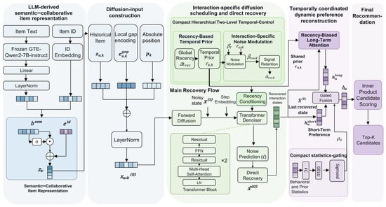
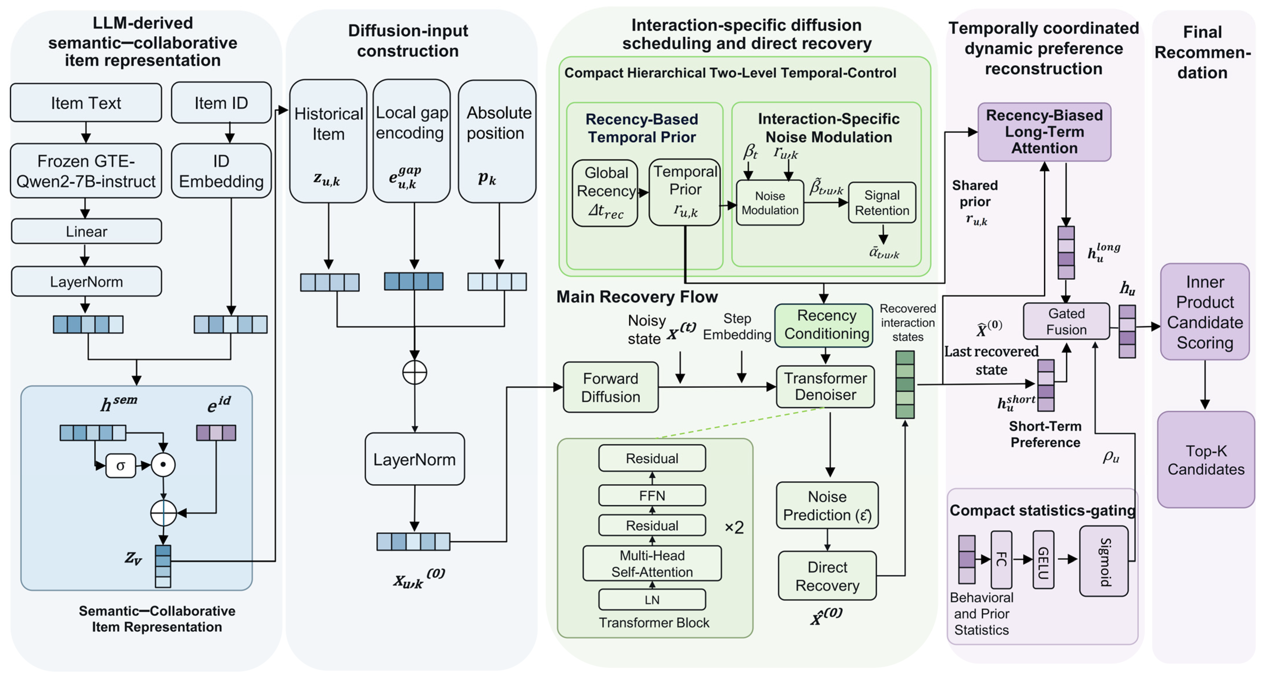
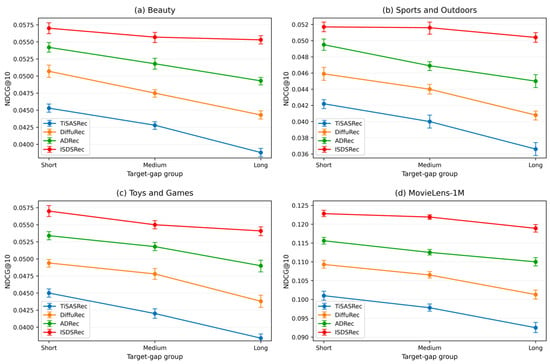
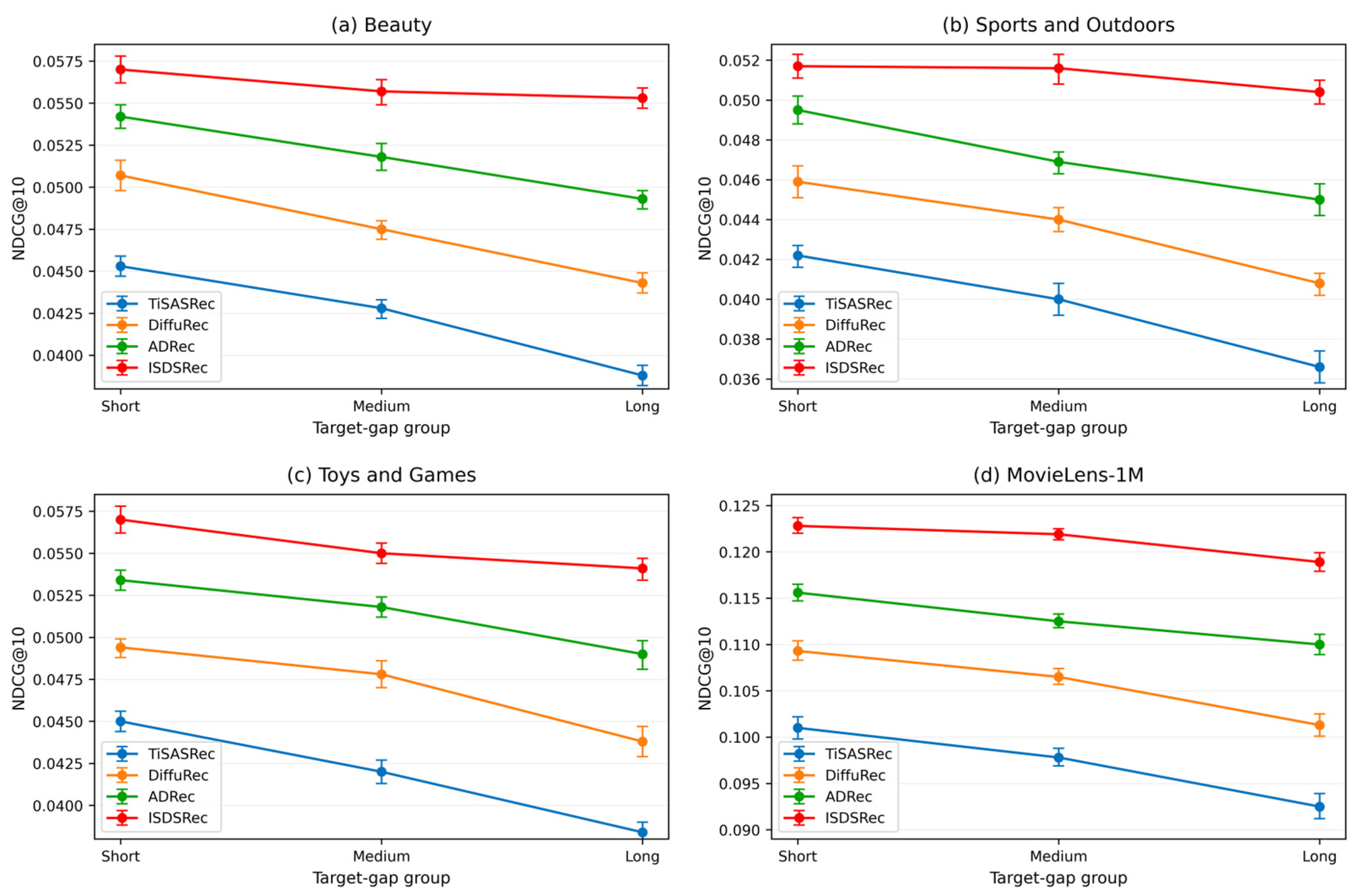
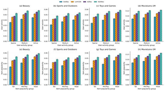
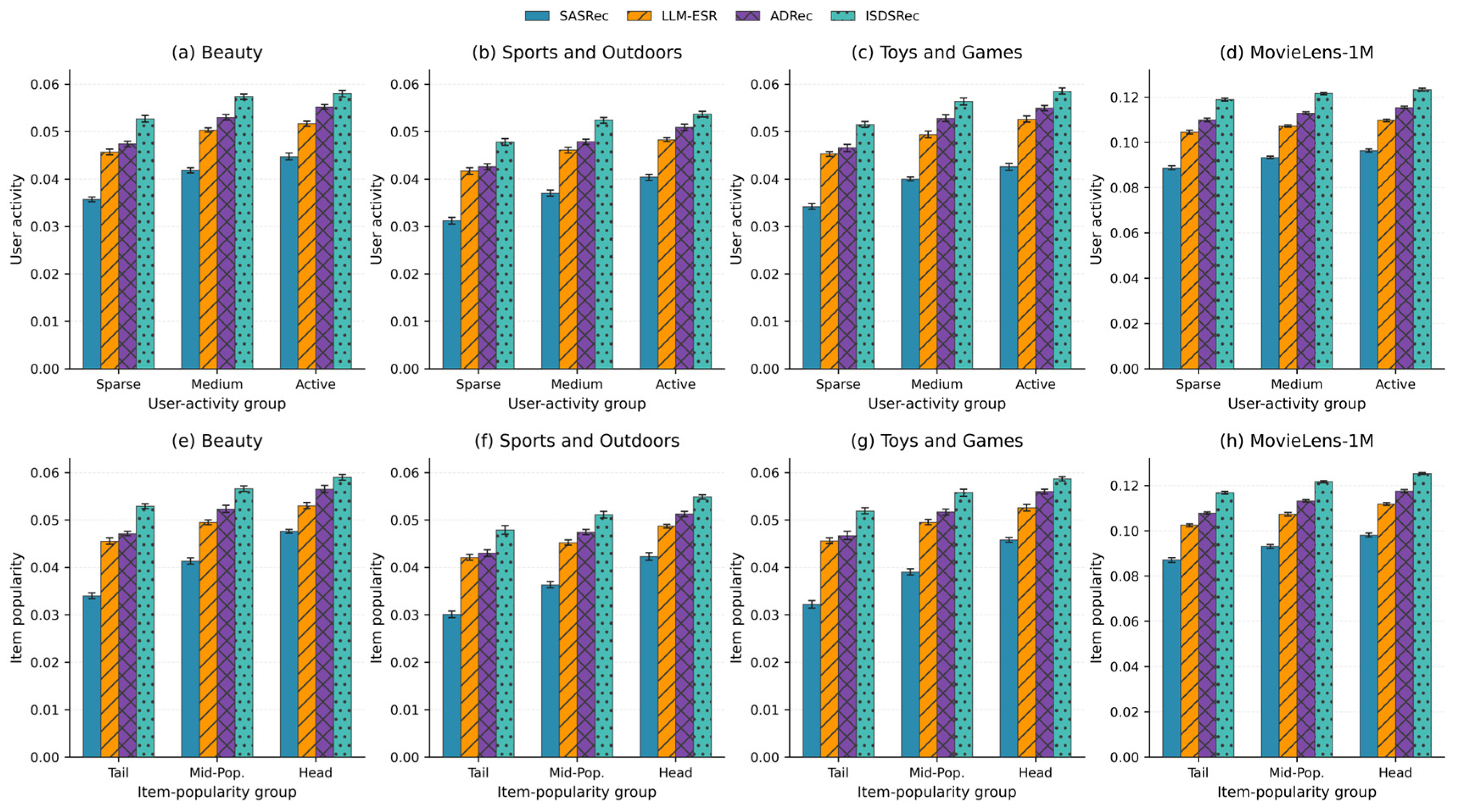
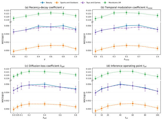
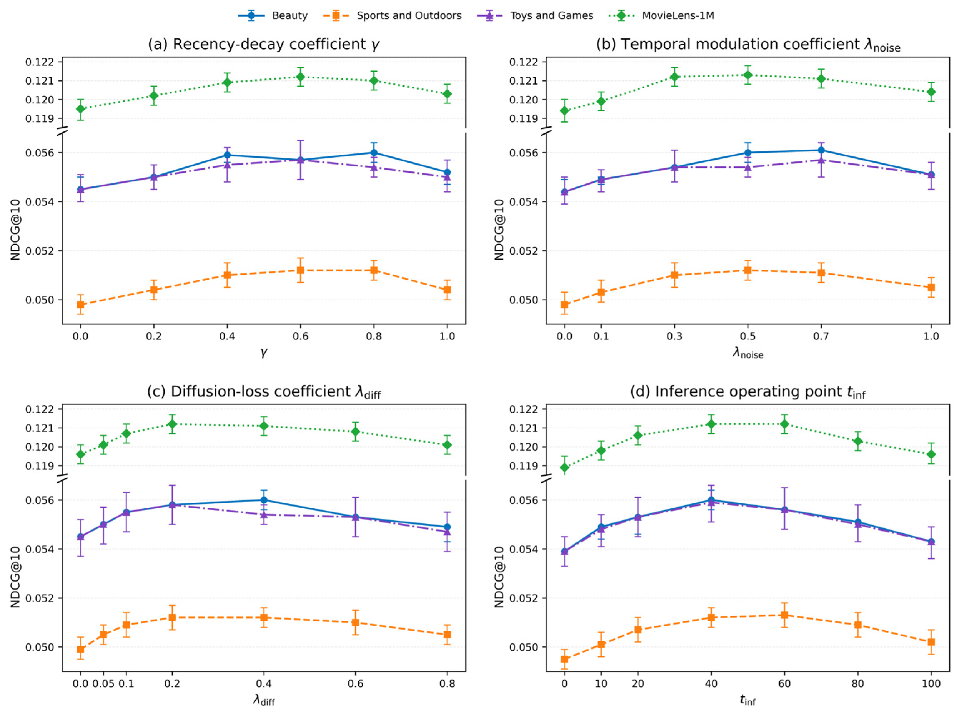

Disclaimer/Publisher’s Note: The statements, opinions and data contained in all publications are solely those of the individual author(s) and contributor(s) and not of MDPI and/or the editor(s). MDPI and/or the editor(s) disclaim responsibility for any injury to people or property resulting from any ideas, methods, instructions or products referred to in the content. |
© 2026 by the authors. Licensee MDPI, Basel, Switzerland. This article is an open access article distributed under the terms and conditions of the Creative Commons Attribution (CC BY) license.