Short-Term Electric Power Load Forecasting Based on ISAO-VMD-BiTCN

Abstract

Aiming to improve short-term power load forecasting under nonlinear and nonstationary load characteristics, this paper develops an Improved Snow Ablation Optimizer (ISAO) and applies it to the hyperparameter optimization of a Variational Mode Decomposition (VMD)- Bidirectional Temporal Convolutional Network (BiTCN) forecasting framework. First, VMD is used to decompose the original load sequence into multiple intrinsic mode function (IMF) components in order to reduce the non-stationarity of the signal. Second, to address the limitations of the Snow Ablation Optimizer (SAO), four strategies—quantum-chaotic hybrid initialization, elite-pool-guided dual-population updating, the quantum tunneling effect, and dynamic lens opposition-based learning—are introduced to form the ISAO algorithm. Finally, ISAO is used to independently optimize the BiTCN hyperparameters of each IMF component, and the prediction results of all components are superimposed and reconstructed to obtain the final forecast. CEC2022 benchmark function tests and experiments on actual load data show that the ISAO algorithm achieves superior optimization performance; compared with the SAO-VMD-BiTCN model, the RMSE of the proposed model decreases from 2342.23 MW to 2202.14 MW, a reduction of 5.98% and the proposed model outperforms comparison models such as VMD-BiTCN and PSO-VMD-BiTCN across the RMSE, MAE, MAPE, and R² metrics. Furthermore, Diebold–Mariano (DM) test results provide additional statistical evidence for the favorable forecasting performance of the proposed framework across multiple random initializations.

1. Introduction

With the deepening advancement of smart grids and new-generation power system construction, short-term electric power load forecasting has become a core supporting technology for ensuring the safe dispatch, economic operation, and efficient market trading of electric power systems [1]. However, power load is influenced by multiple factors such as meteorological conditions, holiday schedules, and socio-economic activity, exhibiting pronounced nonlinearity and non-stationarity, which pose considerable challenges to achieving high-precision forecasting.

In terms of prediction-model architecture, research has also extended beyond conventional recurrent networks. Long Short-Term Memory (LSTM) is a widely used sequence-model baseline that alleviates the vanishing-gradient problem of vanilla RNNs, though a unidirectional LSTM only propagates information forward in time [2]. To better exploit both local and global feature correlations, Cui et al. [3] combined a Convolutional Neural Network (CNN)-based feature-extraction module with a self-attention encoder–decoder network for initial forecasting, followed by a residual-refinement module to further optimize the prediction, reporting improved accuracy and stability. Transformer-based encoder–decoder architectures built purely on self-attention have likewise been applied to load forecasting, offering stronger parallelism and long-range dependency modeling than LSTM [4]. These studies illustrate the potential of convolutional feature extraction, self-attention-based dependency modeling, and residual refinement for improving load forecasting performance. To provide a conventional recurrent baseline, LSTM is also included in the comparative experiments.

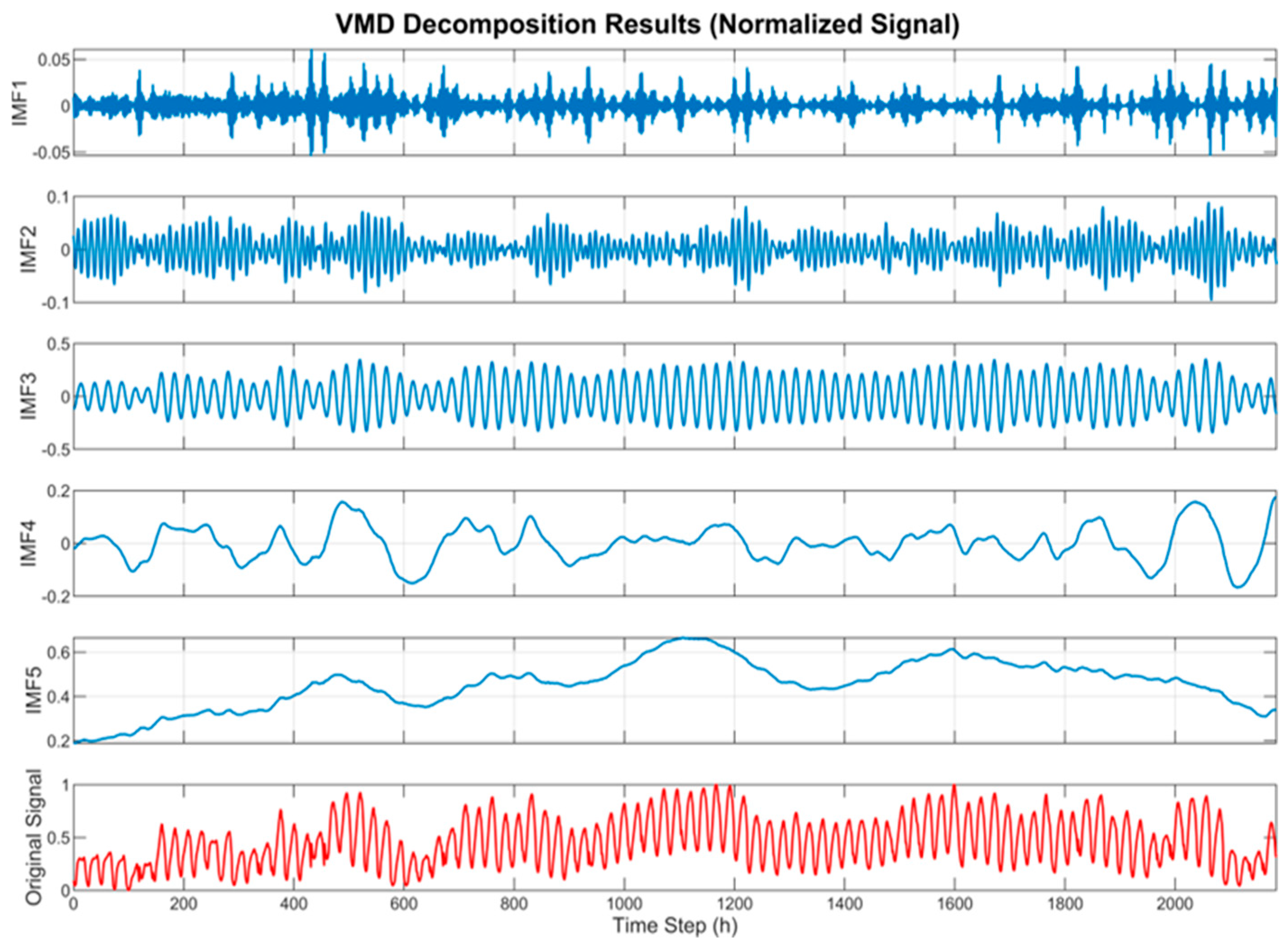
In terms of load-data preprocessing, signal decomposition methods have been widely introduced to reduce the complexity of load sequences. Variational Mode Decomposition (VMD), proposed by Dragomiretskiy et al., converts signal decomposition into a constrained variational problem and iteratively solves for each modal component in the frequency domain via the Alternating Direction Method of Multipliers (ADMM), effectively alleviating the mode-mixing problem of traditional decomposition methods. In recent years, VMD has been widely applied in short-term load forecasting: Yang Huping et al. [5] combined VMD with a CNN- Bidirectional Gated Recurrent Unit (BiGRU) model, reducing the non-stationarity of the load sequence through decomposition and effectively improving prediction accuracy; Wang Qing et al. [6] constructed a VMD- Temporal Convolutional Network (TCN) combined model, confirming that after VMD preprocessing, the frequency-domain characteristics of each component become clearer and prediction performance is significantly better than modeling the raw load sequence directly.

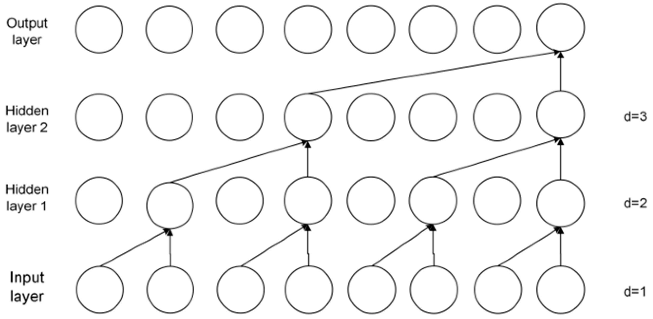
After VMD, the stationarity of the resulting components is markedly improved, and a compatible time-series prediction model is required to achieve high-precision fitting. Regarding prediction models, the TCN, based on dilated causal convolution and residual connections, enables parallel computation while offering a large receptive field and efficient training [7]. Building on this, the Bidirectional Temporal Convolutional Network (BiTCN) proposed by Sprangers et al. further improves prediction performance by modeling bidirectional contextual features in parallel through forward and backward branches [8]. Huang et al. [9] validated the effectiveness of BiTCN in domestic short-term load forecasting; ablation experiments showed that VMD-BiTCN can further reduce prediction error compared with a unidirectional TCN. Fan et al. [10] likewise confirmed that BiTCN, owing to its advantage of processing local features bidirectionally in parallel, performs better within combined prediction models. However, BiTCN hyperparameters such as the number and size of convolution kernels, the dropout rate, and the learning rate significantly affect prediction results, and manual tuning is inefficient and unlikely to yield a globally optimal solution [11].

To address the hyperparameter-optimization problem, metaheuristic algorithms such as Particle Swarm Optimization (PSO) [12], the Grey Wolf Optimizer (GWO) [13], and the Sparrow Search Algorithm (SSA) [14] have been widely used for neural-network hyperparameter tuning. The Snow Ablation Optimizer (SAO) proposed by Deng and Liu, which simulates the sublimation and melting behavior of snow to construct a dual-population cooperative mechanism, achieves an adaptive balance between global exploration and local exploitation [15]. Compared with classical algorithms such as PSO and GWO, it has a stronger ability to escape local optima and performs well on numerical-optimization benchmark tests, indicating good potential for further improvement and application. However, Xiao et al. [16] pointed out that SAO suffers from four shortcomings—uneven initial population distribution, an imbalance between exploration and exploitation, susceptibility to local optima, and insufficient late-stage convergence accuracy; Li et al. [17] likewise confirmed that the excessively strong exploitation capability of SAO leads to an imbalance between global and local search, making it prone to becoming trapped in local extrema in complex scenarios. These issues limit the effectiveness of SAO for BiTCN hyperparameter optimization, making targeted improvement necessary. To address these issues, this paper develops an Improved Snow Ablation Optimizer (ISAO) and applies it to the hyperparameter optimization of a VMD-BiTCN forecasting framework for short-term power load prediction. The main contributions of this paper are summarized as follows:

(1) To address the four documented shortcomings of SAO (uneven initial population distribution, imbalance between exploration and exploitation, susceptibility to local optima, and insufficient late-stage convergence accuracy), four improvement strategies—quantum-chaotic hybrid initialization, elite-pool-guided dual-population updating, the quantum tunneling effect, and dynamic lens opposition-based learning—are introduced to construct the ISAO.

(2) The optimization performance of ISAO is systematically validated on the CEC2022 benchmark functions against RIME, HBA, ARO, and the original SAO, with statistical significance confirmed via the Wilcoxon rank-sum test.

(3) The proposed ISAO is applied to the hyperparameter optimization of a VMD-BiTCN forecasting framework, in which VMD decomposes the load sequence into IMF components and ISAO independently optimizes the BiTCN hyperparameters for each component.

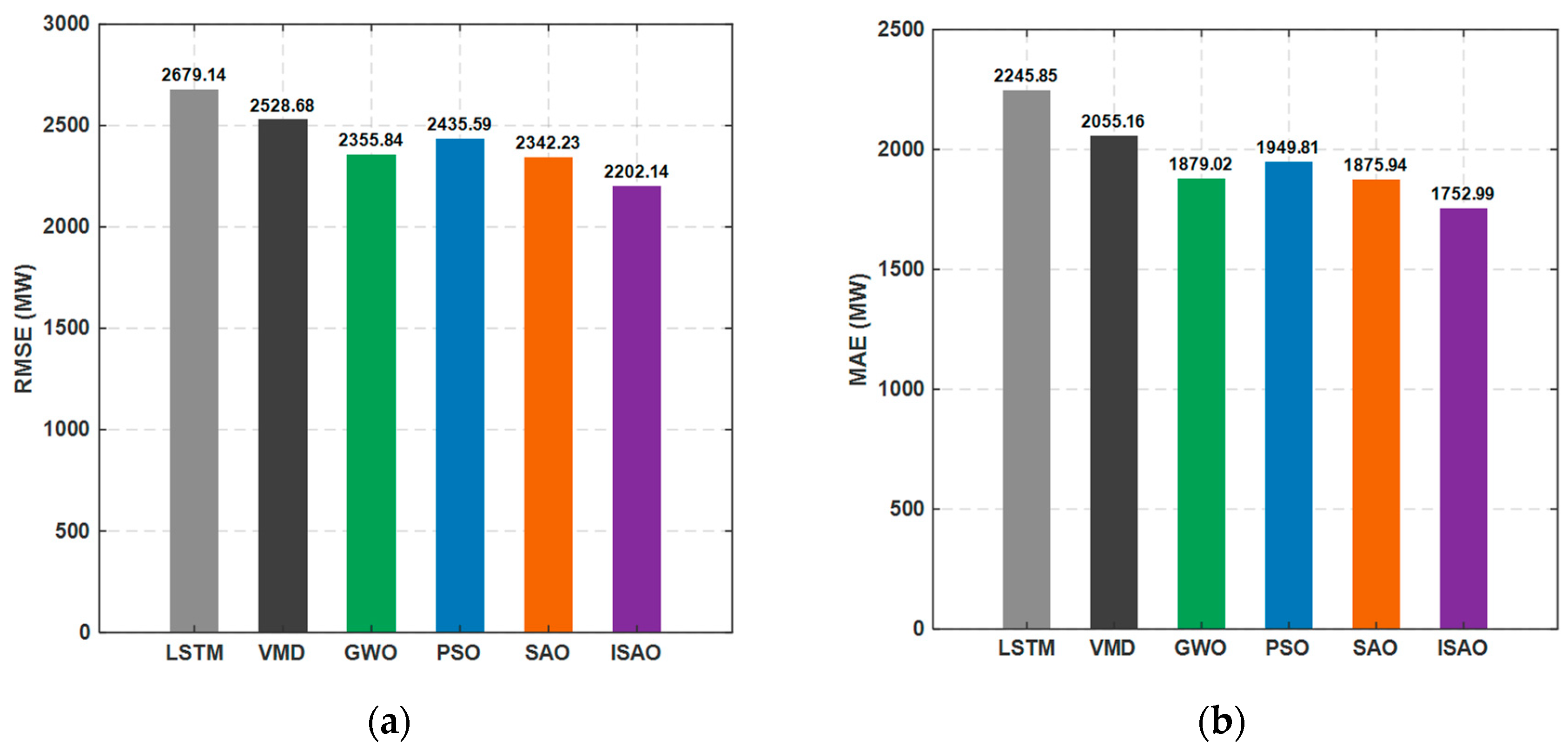
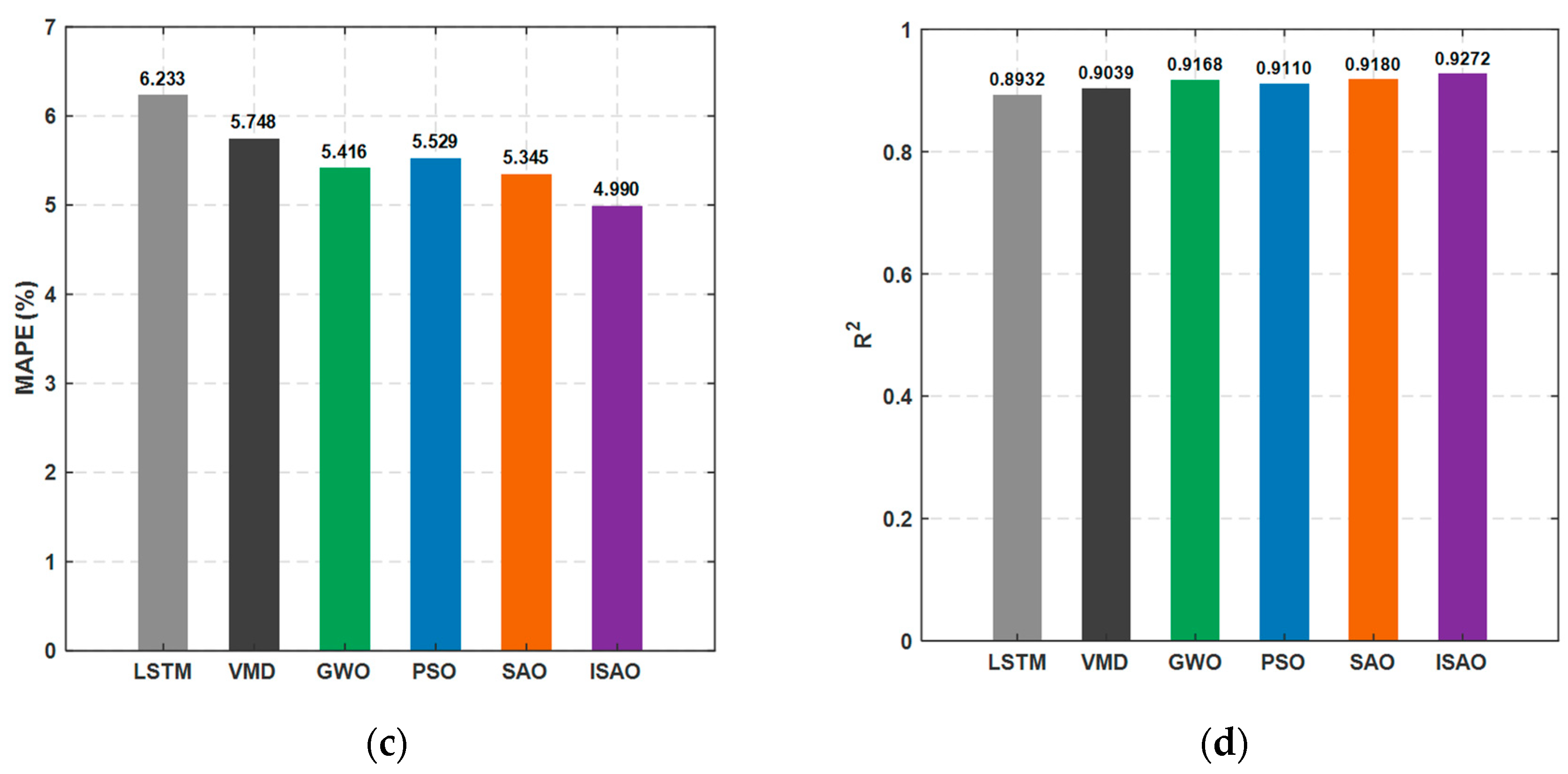
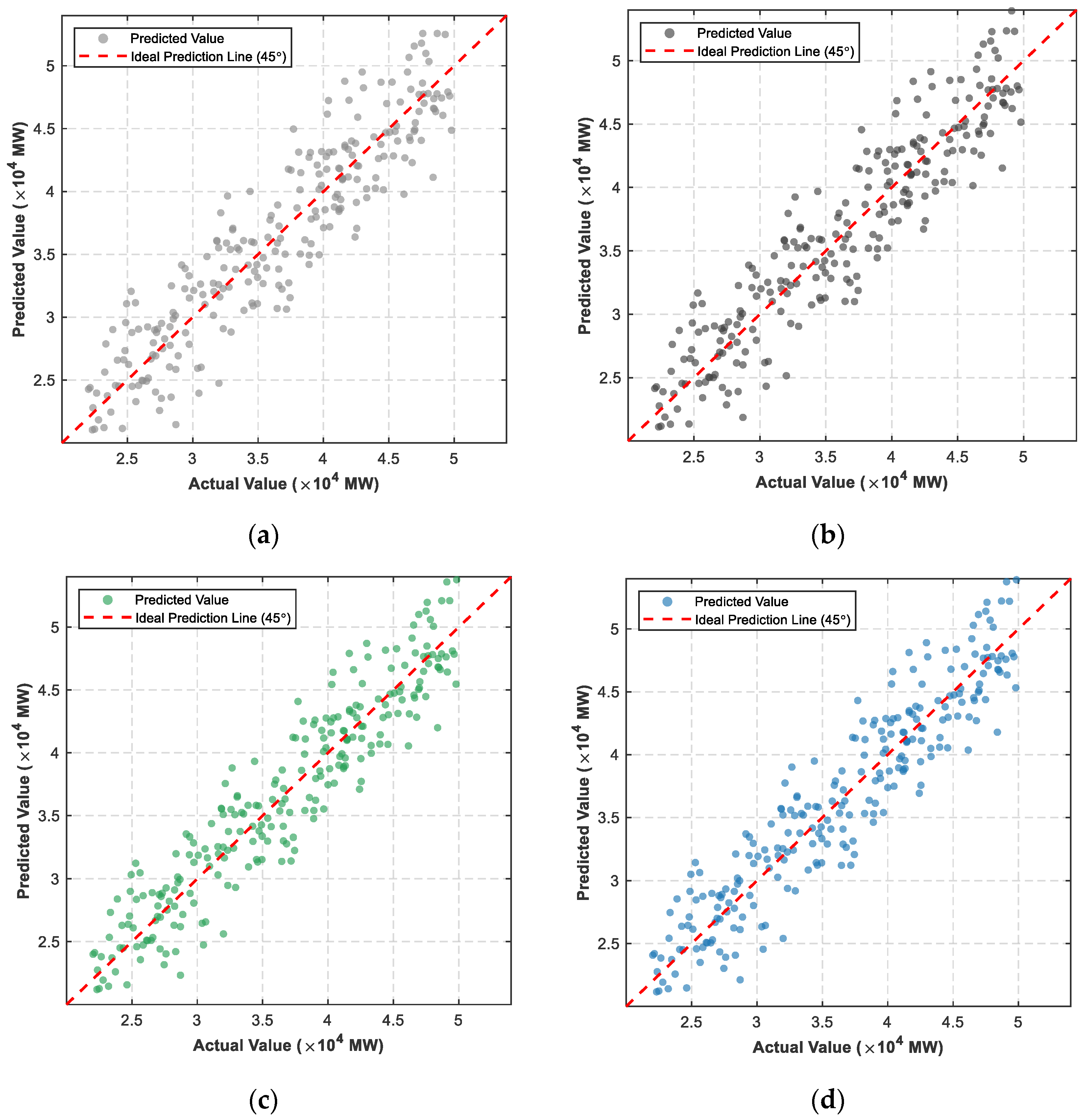
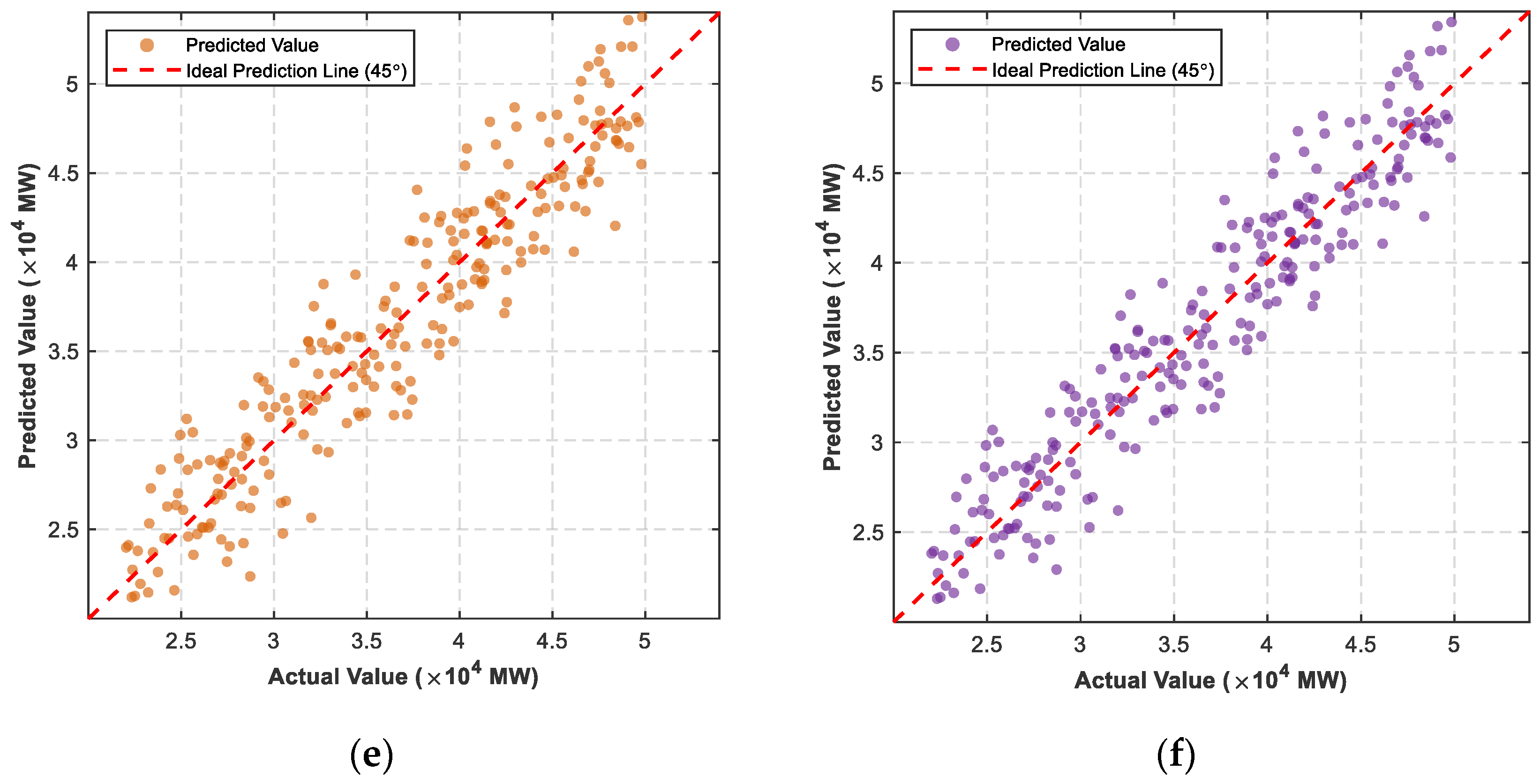
(4) The proposed ISAO-VMD-BiTCN framework is evaluated on real-world PJM load data against LSTM, VMD-BiTCN, GWO-VMD-BiTCN, PSO-VMD-BiTCN, and SAO-VMD-BiTCN, achieving the best overall performance among the compared forecasting models in terms of RMSE, MAE, MAPE, and R².

The remainder of this paper is organized as follows. Section 2 introduces VMD and its role in reducing the non-stationarity of the original load sequence. Section 3 presents the BiTCN, which serves as the prediction backbone for each decomposed component. Section 4 reviews the SAO and details the proposed ISAO, which is used to automatically optimize the BiTCN hyperparameters. Section 5 integrates VMD, BiTCN, and ISAO into the proposed combined prediction model. Section 6 validates the proposed model on real-world PJM load data through comparative case studies against four benchmark models. Section 7 concludes the paper.

2. VMD

As the data-preprocessing stage of the proposed ISAO-VMD-BiTCN framework, this section introduces VMD, which is used to decompose the original load sequence into components with reduced non-stationarity. VMD decomposes the original load sequence f into K intrinsic mode function (IMF) components $u_k(t)$, each with an independent center frequency and a limited bandwidth. Its constrained variational objective function is expressed as:

$$\begin{array}{c}min\\ \left\{u_k\right\},\left\{w_k\right\}\end{array}\left\{{\displaystyle \sum _{k=1}^K}{‖{\partial }_t\left[\left(\delta (t)+{\displaystyle \frac{j}{\pi t}}\right)\ast u_k(t)\right]e^{-j{w}_{k}t}‖}_2^2\right\}$$

(1)

$$s.t.{\displaystyle \sum _{k=1}^K}{u}_k(t)=f(t)$$

where $\left\{u_k\right\}$ denotes the decomposed modal components; $\left\{w_k\right\}$ denotes the center frequency of each component; $\delta (t)$ is the Dirac function; and $\ast$ denotes the convolution operation. Using a quadratic penalty factor $\alpha$ and Lagrange multiplier $\lambda (t)$, this constrained problem is converted into an unconstrained one and solved iteratively in the frequency domain via the Alternating Direction Method of Multipliers (ADMM).

In practical application, the number of decomposed modes K and the penalty factor $\alpha$ are the key parameters governing decomposition quality. This paper determines K using the center-frequency observation method, progressively increasing K while observing the distribution of the center frequencies of each IMF. Experiments show that when K = 5, the center frequencies of the components are evenly distributed with no overlap; the penalty factor $\alpha$ is set to its default value of 2000. Under these settings, the maximum VMD reconstruction error is only $4.52\times {10}^{-2}$, indicating that the decomposition accuracy fully satisfies the requirements of subsequent forecasting.

3. BiTCN Network

Section 2 decomposed the original load sequence into IMF components via VMD; this section introduces the BiTCN network, which serves as the prediction backbone for each of these components. BiTCN consists of two parallel branches: a forward TCN and a backward TCN. The forward TCN performs causal convolution on the input sequence in chronological order, while the backward TCN performs causal convolution after reversing the input sequence in time, thereby implicitly capturing the future context of the sequence. The core modules of TCN comprise three key techniques: causal convolution, dilated convolution, and residual connections. For an input sequence $x=(x_0,x_1,\cdots ,x_t)$, the corresponding output $y=(y_0,y_1,\cdots {,y}_t)$ after causal convolution is:

$$y_t=f_c(x_0,x_1,x_2,\cdots ,x_t)$$

(2)

where $f_c$ denotes the causal convolution operation.

The dilated convolution structure is shown in Figure 1. For an input sequence $x=(x_0,x_1,\cdots ,x_t)$, the hidden-layer output after dilated convolution is:

$$F^{(l)}(t)={\displaystyle \sum _{i=0}^{k_c-1}}{w}^{(l)}(i)·x_{t-d^{(l)}·i}$$

(3)

where $k_c$ is the convolution kernel size, $w^{(l)}$ is the $i-th$ trainable kernel coefficient at layer $l,$ and $d^{(l)}$ is the layer-dependent dilation factor, with $d^{(1)}=1$, $d^{(2)}=2$, $d^{(3)}=3,$ as shown in Figure 1. This dilated convolution module is shared by the forward and backward branches of BiTCN.

The residual connection adds the input $x$ to the nonlinearly transformed $F(x)$:

$$y=F(x)+x$$

(4)

4. Snow Ablation Optimizer and Its Improvement

Because BiTCN’s prediction accuracy is highly sensitive to hyperparameter choices, this section focuses on their optimization: Section 4.1 reviews the original SAO, and Section 4.2 develops the proposed ISAO, which is later used to automatically tune these hyperparameters for each IMF component.

4.1. Snow Ablation Optimizer (SAO)

SAO is a metaheuristic developed by Deng and Liu that simulates the sublimation and melting of accumulated snow to achieve a trade-off between exploration and exploitation, thereby avoiding premature convergence. SAO mainly consists of an initialization stage, an exploration stage, an exploitation stage, and a dual-population mechanism.

4.1.1. Initialization Stage

In SAO, the iterative process begins with a randomly generated population. As shown below, the entire population is typically modeled as a matrix with $N$ rows and $Dim$ columns, where $N$ represents the population size, and $Dim$ represents the dimensionality of the solution space.

$$Z=lb+\theta \times (ub-lb)={\left[\begin{array}{ccccc}{Z}_{\mathrm{1,1}}& Z_{1,2}& \cdots & Z_{1,Dim-1}& Z_{1,Dim}\\ Z_{2,1}& Z_{2,2}& \cdots & Z_{2,Dim-1}& Z_{2,Dim}\\ ⋮& ⋮& \ddots & ⋮& ⋮\\ Z_{N-\mathrm{1,1}}& Z_{N-\mathrm{1,2}}& \cdots & Z_{N-1,Dim-1}& Z_{N-1,Dim}\\ Z_{N,1}& Z_{N,2}& \cdots & Z_{N,Dim-1}& Z_{N,Dim}\end{array}\right]}_{N\times Dim}$$

(5)

where $lb$ and $ub$ denote the lower and upper bounds of the solution space, respectively, and $\theta$ denotes a random number in [0, 1].

4.1.2. Exploration Stage

When snow, or the liquid water converted from snow, turns into vapor, the individuals exhibit highly dispersed characteristics owing to irregular motion. In this study, Brownian motion is used to simulate this behavior. As a stochastic process, Brownian motion is widely used to model animal foraging behavior, the ceaseless and irregular motion of particles, stock-price fluctuations, and similar phenomena. For standard Brownian motion, the step length is obtained from the probability density function of a normal distribution with mean 0 and variance 1, expressed as follows:

$$f_{BM}(x;0,1)={\displaystyle \frac{1}{\sqrt{2\pi }}}\times exp(-{\displaystyle \frac{x^2}{2}})$$

(6)

Brownian motion can explore potential regions of the search space and therefore effectively reflects the diffusion of vapor within it. The position-update formula during the exploration process is:

$$Z_i(t+1)=Elite(t)+B{M}_i(t)⨂\left({\theta }_1\times \left(G(t)-Z_i(t)\right)+\left(1-{\theta }_1\right)\times \left(\overline{Z}(t)-Z_i(t)\right)\right)$$

(7)

$$\overline{Z}(t)={\displaystyle \frac{1}{N}}{\displaystyle \sum _{i=1}^N}{Z}_i(t)$$

(8)

$$Elite(t)\in \left[G(t),Z_{second}(t),Z_{third}(t),Z_c(t)\right]$$

(9)

$$Z_c(t)={\displaystyle \frac{1}{N_1}}{\displaystyle \sum _{i=1}^{N_1}}{Z}_i(t)$$

(10)

where $Z_i(t+1)$ is the position of the $i-th$ individual at time $t+1$; $Elite(t)$ is a random variable selected from among $G(t)$, $Z_{second}(t)$, $Z_{third}(t)$ and $Z_c(t)$; $B{M}_i$ is a Brownian-motion coefficient governing the random-walk step of the $i-th$ individual; $G(t)$ is the position of the best individual at time $t$; $Z_{second}(t)$ and $Z_{third}(t)$ are the second-best and third-best positions at time $t$; and $Z_c(t)$ is the average position of the individuals at time $t$.

4.1.3. Exploitation Stage

When snow is converted into liquid water through melting, this process is simulated according to the snow-ablation process as follows:

$$M=DDF\times (T-T_1)$$

(11)

where $DDF$ is the snow-ablation coefficient, ranging over [0.35, 0.6]; $T$ is the daily average temperature (°C); and $T_1$ is the base temperature (°C). $DDF$ varies with time as:

$$DDF=0.35+0.25\times {\displaystyle \frac{e^{\frac{t}{t_{max}}-1}}{e-1}}$$

(12)

The position is then updated to simulate the snow-ablation process:

$$Z_i(t+1)=M\times G(t)+B{M}_i(t)⨂\left({\theta }_2\times \left(G(t)-Z_i(t)\right)+\left(1-{\theta }_2\right)\times \left(\overline{Z}(t)-Z_i(t)\right)\right)$$

(13)

where $M$ is the snow-ablation rate and ${\theta }_2$ is a random number in the range [−1, 1].

4.1.4. Dual-Population Mechanism

In SAO, balancing the exploration and exploitation stages prevents the algorithm from converging prematurely and enables a more comprehensive search of the solution space in pursuit of the global optimum. Accordingly, in the early stage of iteration, SAO achieves this balance by introducing a dual-population mechanism, whereby the entire population is randomly divided into two subgroups of equal size.

4.2. Improved Snow Ablation Optimizer (ISAO)

4.2.1. Quantum-Chaotic Hybrid Initialization Strategy

Although SAO is simple to implement, it is prone to population clustering in high-dimensional search spaces, resulting in insufficient search coverage and a reduced probability of locating the global optimum. To address this, a quantum-chaotic hybrid initialization strategy is introduced. This strategy uses the quantum logistic map as the chaotic source, with the iterative formula:

$$q(n+1)=\mu ·q(n)·(1-q(n))·(1-2·{\left|q(n)\right|}^2)$$

(14)

where $q(n)\in (0, 1)$ is the quantum-state amplitude at step n; $\mu \in (3.57,4]$ is the chaos control parameter, set to $\mu =4$ in this paper to guarantee full chaotic behavior; and ${\left|q(n)\right|}^2$ is the squared modulus of the quantum-state probability amplitude, introduced so that the map possesses quantum ergodicity beyond that of the classical logistic map, enabling more uniform probability coverage of the [0, 1] interval. After generating the chaotic-sequence operator $Q_{chaos}$ from the above sequence, the initial population is mapped into the search space as follows:

$$x_i=lb+Q_{chaos}\times \left(ub-lb\right)$$

(15)

where $Q_{chaos}$ denotes the operator generated by the quantum-chaotic map. This effectively increases population diversity and lays the foundation for subsequent global exploration.

4.2.2. Elite-Pool-Guided Dual-Population Update Mechanism

To strengthen the guidance of the search process, ISAO constructs an elite pool composed of the best individual $Z_{best}$, the second-best individual $Z_{second}$, the third-best individual $Z_{third}$ and the centroid $Z_{centroid}$ of the top 50% of individuals. Building on this, a hierarchical dual-population update mechanism is designed, randomly dividing the population into an elite-guided subset $N_a$ and a dynamic-scaling subset $N_b$.

The elite-guided subset $(N_a)$ corresponds to the SAO exploration-stage formula, while retaining its Brownian-motion framework and weighted-displacement structure, the fixed elite term $Elite(t)$ is extended to a guidance term dynamically sampled from the elite pool E_p, enhancing the diversity of exploration directions.

$$Z_i(t+1)=E_p(K)+RB⨂\left[r_1\times \left(Z_{best}-Z_i(t)\right)+(1-r_1)\times (Z_{centroid}-Z_i(t))\right]$$

(16)

where $E_p(K)$ is the k-th elite individual randomly selected from the elite pool; $r_1\in [-1, 1]$ corresponds to ${\theta }_1$ in the original formula; $Z_{centroid}$ is the population centroid, corresponding to $\overline{Z}(t)$ and $Z_{best}$ corresponds to $G(t)$. $RB$ is a random perturbation vector following Brownian motion, with each element independently drawn from a standard normal distribution. $⨂$ denotes the Hadamard product.

The dynamic-scaling subset $(N_b)$ corresponds to the SAO exploitation-stage formula, while retaining its snow-ablation coefficient M and weighted-displacement framework, a temperature factor $T$ is introduced to dynamically adjust the update speed, enabling the algorithm to transition smoothly from early-stage global exploration to late-stage local exploitation:

$$Z_i(t+1)=M\times Z_{best}+RB⨂\left[r_2\times \left(Z_{best}-Z_i(t)\right)+\left(1-r_2\right)\times \left(Z_{centroid}-Z_i(t)\right)\right]$$

(17)

$$\tau =exp\left({\displaystyle \frac{-t}{Maxiter}}\right)$$

(18)

where $M$ is the snow-ablation rate; $r_2\in [-1, 1]$ corresponds to ${\theta }_2$ in the original formula; $\tau$ is the temperature factor; $t$ is the current iteration number; and $Maxiter$ is the maximum number of iterations. $\tau$ decreases nonlinearly from 1 to $e^{-1}\approx 0.368$ as iterations proceed, allowing the dynamic-scaling subset to maintain a larger update step in the early iterations for thorough exploration, and to gradually contract in later iterations to focus on local exploitation, thereby achieving a dynamic balance between exploration and exploitation.

4.2.3. Quantum Tunneling Effect Exploration Strategy

To break through local extrema in the search space, a quantum tunneling effect mechanism is introduced. This mechanism allows an individual to cross the current search region with a certain probability $P_{tunnel}$ and perform a large-scale jump.

$P_{tunnel}$ is dynamically adjusted as iterations proceed, being larger in the early stage to maintain search intensity and lower in the later stage to focus on exploitation:

$$P_{tunnel}=0.25\times {\left(1-{\displaystyle \frac{t}{Maxiter}}\right)}^2+0.05$$

(19)

When the tunneling effect is triggered, an individual performs the following jump:

$$Z_{tunnel}=X_i+S_j\times \left(ub-lb\right)\times \left(rand-0.5\right)$$

(20)

$S_j$ is the jump intensity, which decreases dynamically with the iteration number, calculated as:

$$S_j=S_{max}·\left(1-{\displaystyle \frac{t}{Maxiter}}\right)+S_{min}$$

(21)

where $S_{max}=$0.2 is the maximum jump intensity; $S_{min}=0.01$ is the lower bound of the jump intensity; and $t$ is the current iteration number. $S_j$ decreases linearly, providing relatively large jump steps in the early stage to help individuals cross local barriers and explore the search space, while gradually reducing the jump range in the later stage to minimize disturbance to promising solutions.$rand\in [0, 1]$ is a uniformly distributed random number. This strategy grants individuals a “tunneling” capability, effectively guiding the population to escape local optima in which it has become stagnant and substantially enhancing the algorithm’s global search capability.

4.2.4. Dynamic Lens Opposition-Based Learning

To further improve the convergence accuracy of the algorithm, dynamic lens opposition-based learning is introduced at the end of the iterative process. By generating an opposition-based solution near the current optimum and deciding, via a greedy selection strategy, whether to replace the current optimum with this solution, a refined search of the neighborhood of the optimal solution is achieved. A dynamic-scaling factor $d_K$ is introduced to control the search range of the opposition-based solution, allowing it to cover a larger region in the early stage of iteration and progressively narrow in the later stage.

$$d_K={10}^4\times \left(1-{\left({\displaystyle \frac{t}{Maxiter}}\right)}^2\right)+1$$

(22)

Based on the principle of lens imaging, the opposition-based solution is calculated as:

$$Z_{best}^{\prime }={\displaystyle \frac{ub+lb}{2}}+{\displaystyle \frac{ub+lb}{2\ast d_K}}-{\displaystyle \frac{Z_{best}}{d_K}}$$

(23)

where $d_K$ decreases as the iteration number increases, allowing the opposition-based solution to gradually contract toward the neighborhood of $Z_{best}$ in the later stage and achieve refined exploitation. If the fitness of $Z_{best}^{\prime }$ is better than that of $Z_{best}$, the current best solution is updated; otherwise, the original best solution is retained. This greedy selection ensures that the best-so-far fitness does not deteriorate during the update.

4.3. Performance Testing

This paper uses the CEC2022 benchmark test function set (F1–F12) to evaluate the performance of the proposed ISAO algorithm. The experimental parameters are set as follows: population size 30, maximum number of iterations 500, problem dimension 10, and 30 independent runs. The comparison algorithms include the Rime Ice Algorithm (RIME) [18], the Honey Badger Algorithm (HBA) [19], Artificial Rabbit Optimization (ARO) [20], and SAO. The statistical indicators include the minimum value (Min), standard deviation (Std), mean value (Avg), median (Median), and worst value (Worst).

Table 1. Statistical comparison of CEC2022 benchmark function results.

Func	Metric	ISAO	RIME	HBA	ARO	SAO
	Min	300.0003	300.0908	300.0002	304.7959	300.0260
	Std	3.7548	0.7092	0.1252	191.6372	1.5922 × 103
F1	Avg	301.3804	300.9447	300.0452	492.1757	990.9372
	Median	300.1449	300.6781	300.0086	451.1535	567.3950
	Worst	319.9029	303.2662	300.6727	988.4204	8.7853 × 103
	Min	400.0994	400.0331	400.0010	400.0008	400.0061
	Std	1.9507	15.7973	22.8777	17.4218	3.2856
F2	Avg	404.9227	410.3404	415.0236	407.6390	406.3220
	Median	404.7841	407.5445	408.9161	400.7275	408.9161
	Worst	407.5227	470.2210	475.6756	471.1503	408.9161
	Min	600.0000	600.0589	600.0043	600.0013	600.0000
	Std	7.7407 × 10−5	0.2808	1.6482	0.5668	0.0352
F3	Avg	600.0000	600.2744	600.9259	600.2105	600.0090
	Median	600.0000	600.2258	600.1995	600.0280	600.0000
	Worst	600.0004	601.5666	607.4770	602.8726	600.1734
	Min	802.9966	807.9627	806.9647	803.9799	801.9899
	Std	6.8525	13.1978	6.6797	6.2618	8.2546
F4	Avg	811.0183	828.0266	818.2610	815.9582	813.6012
	Median	809.5156	823.2814	818.4067	815.0092	812.4370
	Worst	828.7462	861.6931	830.8437	828.8538	844.7360
	Min	900.0000	900.0062	900.0000	900.0001	900.0000
	Std	1.0381	6.1228	38.2611	21.1273	0.1660
F5	Avg	900.4601	902.6485	926.1769	914.8638	900.0693
	Median	900.0000	900.7311	912.9602	904.8294	900.0000
	Worst	904.0415	933.5265	1.0718 × 103	985.3316	900.6334
	Min	1.9620 × 103	1.8378 × 103	1.8491 × 103	1.8124 × 103	1.8188 × 103
	Std	2.1894 × 103	2.0025 × 103	2.1889 × 103	1.5152 × 103	2.0880 × 103
F6	Avg	4.2327 × 103	4.1825 × 103	4.1042 × 103	2.8117 × 103	3.9603 × 103
	Median	3.9154 × 103	3.8159 × 103	3.2090 × 103	2.1365 × 103	3.4378 × 103
	Worst	1.2590 × 103	8.1163 × 103	8.2302 × 103	6.7019 × 103	7.6322 × 103
	Min	2.0002 × 103	2.0004 × 103	2.0020 × 103	2.0000 × 103	2.0010 × 103
	Std	9.0641	8.4490	5.9113	8.9392	23.8749
F7	Avg	2.0163 × 103	2.0167 × 103	2.0231 × 103	2.0149 × 103	2.0234 × 103
	Median	2.0212 × 103	2.0211 × 103	2.0226 × 103	2.0201 × 103	2.0216 × 103
	Worst	2.0278 × 103	2.0243 × 103	2.0369 × 103	2.0216 × 103	2.1443 × 103
	Min	2.2033 × 103	2.2006 × 103	2.2010 × 103	2.2009 × 103	2.2007 × 103
	Std	7.2393	6.7222	43.8477	6.5225	23.2900
F8	Avg	2.2237 × 103	2.2187 × 103	2.2347 × 103	2.2182 × 103	2.2228 × 103
	Median	2.2270 × 103	2.2212 × 103	2.2226 × 103	2.2207 × 103	2.2205 × 103
	Worst	2.2310 × 103	2.2222 × 103	2.4331 × 103	2.2217 × 103	2.3428 × 103
	Min	2.4856 × 103	2.5293 × 103	2.5293 × 103	2.5293 × 103	2.5293 × 103
	Std	2.8769	26.8256	26.6758	26.8239	0
F9	Avg	2.4874 × 103	2.5342 × 103	2.5352 × 103	2.5342 × 103	2.5293 × 103
	Median	2.4859 × 103	2.5293 × 103	2.5298 × 103	2.5293 × 103	2.5293 × 103
	Worst	2.4956 × 103	2.6762 × 103	2.6762 × 103	2.6762 × 103	2.5293 × 103
	Min	2.5002 × 103	2.4436 × 103	2.5003 × 103	2.5002 × 103	2.5002 × 103
	Std	46.3805	65.0293	155.8920	49.2271	56.3875
F10	Avg	2.5231 × 103	2.5505 × 103	2.5988 × 103	2.5272 × 103	2.5425 × 103
	Median	2.5004 × 103	2.5006 × 103	2.6125 × 103	2.5005 × 103	2.5005 × 103
	Worst	2.6253 × 103	2.6475 × 103	3.3686 × 103	2.6233 × 103	2.6252 × 103
	Min	2.6000 × 103	2.6249 × 103	2.6000 × 103	2.6000 × 103	2.6000 × 103
	Std	131.2797	94.6216	166.5669	129.3503	126.5838
F11	Avg	2.7289 × 103	2.9059 × 103	2.7078 × 103	2.6858 × 103	2.8001 × 103
	Median	2.7504 × 103	2.9222 × 103	2.6000 × 103	2.6006 × 103	2.9000 × 103
	Worst	3.0004 × 103	3.1715 × 103	3.1835 × 103	2.9122 × 103	2.9000 × 103
	Min	2.8476 × 103	2.8614 × 103	2.8605 × 103	2.8643 × 103	2.8614 × 103
	Std	4.0511	3.2534	29.8124	1.9350	4.1797
F12	Avg	2.8502 × 103	2.8667 × 103	2.8885 × 103	2.8673 × 103	2.8658 × 103
	Median	2.8487 × 103	2.8663 × 103	2.8831 × 103	2.8671 × 103	2.8649 × 103
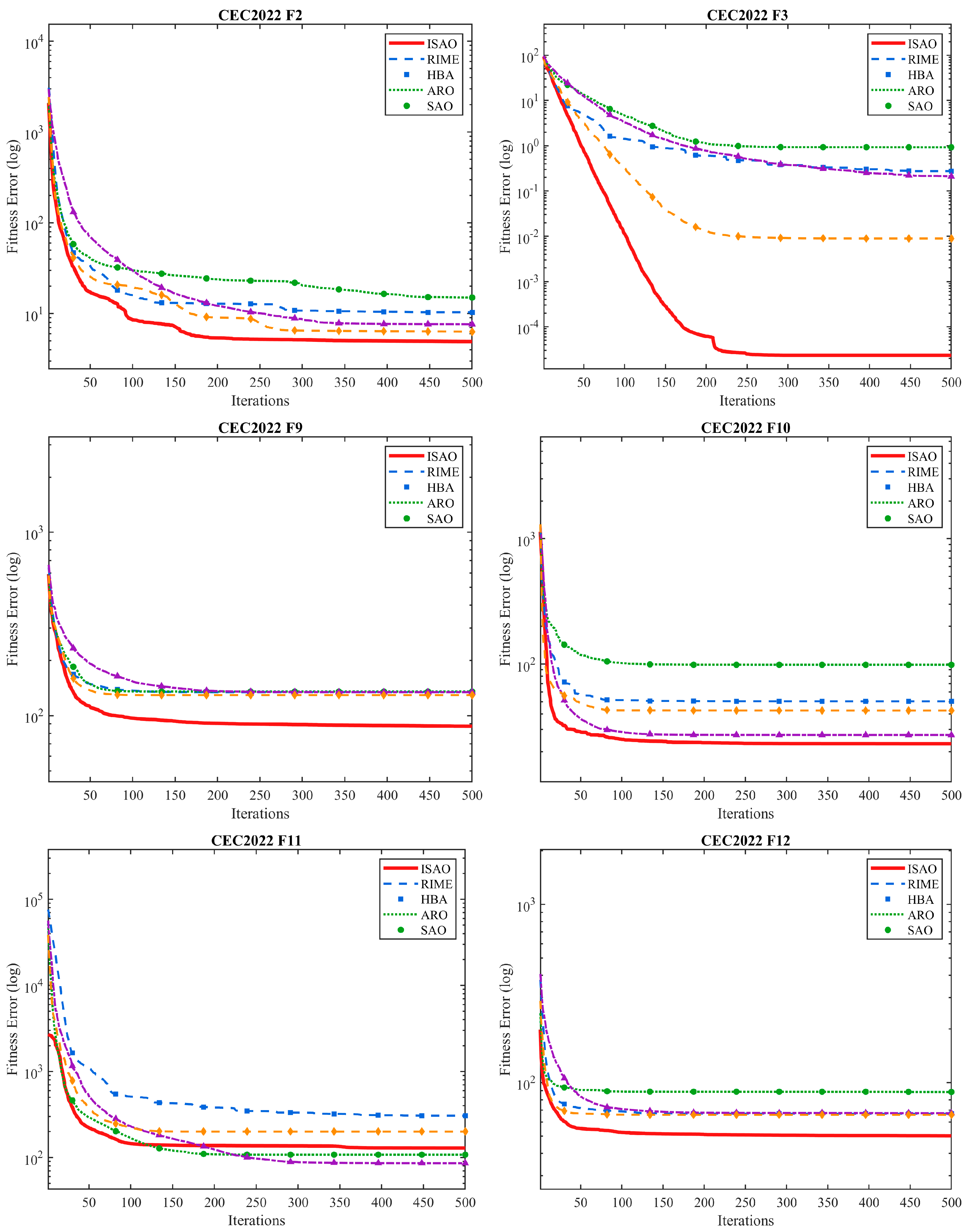
	Worst	2.8651 × 103	2.8786 × 103	3.0004 × 103	2.8728 × 103	2.8845 × 103

presents the statistical results of each algorithm on the CEC2022 benchmark functions F1–F12.

Taken together, the results in Table 1 and Figure 2 show that ISAO achieves substantial improvement over the original SAO while maintaining competitive optimization performance across the CEC2022 benchmark suite. A particularly notable improvement is observed on F1, where the average value decreases from 990.9372 for SAO to 301.3804 for ISAO, corresponding to a reduction of approximately 69.58%. ISAO achieves the best average and median results among all compared algorithms on six test functions, namely F2, F3, F4, F9, F10, and F12. On F3, ISAO reaches the theoretical optimum of 600 with a very small standard deviation, indicating accurate and stable optimization performance. The convergence curves in Figure 2 further show that ISAO generally achieves rapid improvement during the early iterations and maintains a stable convergence trend thereafter.

Nevertheless, the performance of ISAO remains dependent on the characteristics of individual benchmark functions. For F6, ARO achieves substantially better performance than ISAO, with average values of 2811.7 and 4232.7, respectively, and the difference is statistically significant. On F7, ARO also achieves a lower average value than ISAO, with a statistically significant difference. For F11, both ARO and HBA obtain lower average values than ISAO, with average values of 2685.8, 2707.8, and 2728.9 for ARO, HBA, and ISAO, respectively. However, the differences between ISAO and ARO and between ISAO and HBA are not statistically significant. These results suggest that different metaheuristic search mechanisms may exhibit different levels of adaptability to individual benchmark landscapes. In particular, the search strategies incorporated into ISAO improve the overall search capability of SAO, but their effectiveness may vary across functions with different modality, ruggedness, and local-optimum distributions. Therefore, the benchmark results demonstrate clear improvements of ISAO over the original SAO and strong competitiveness across a broad range of functions, rather than universal superiority on every test function.

4.4. Wilcoxon Rank-Sum Test

To scientifically assess whether the performance improvement of ISAO is statistically significant, this section adopts the Wilcoxon rank-sum test at a significance level of α = 0.05. The calculated p-values are given in

Table 2. Wilcoxon rank-sum test p-values.

Func	RIME	HBA	ARO	SAO
F1	0.0014	7.2208 × 10−6	6.6955 × 10−11	1.4294 × 10−8
F2	0.0035	0.0058	0.1260	0.0114
F3	2.5158 × 10−11	2.5158 × 10−11	2.5158 × 10−11	0.0032
F4	5.0922 × 10−8	1.7836 × 10−4	0.0046	0.2339
F5	5.2943 × 10−6	2.8725 × 10−9	8.4372 × 10−8	1.0000
F6	0.9941	0.6627	4.2175 × 10−5	0.3632
F7	0.4464	0.0030	0.0378	0.2581
F8	8.1465 × 10−5	0.2170	7.1988 × 10−5	4.7138 × 10−4
F9	3.0199 × 10−11	2.5562 × 10−11	3.0199 × 10−11	1.2118 × 10−12
F10	0.0012	1.5846 × 10−4	0.0035	0.0850
F11	2.0035 × 10−8	0.0962	0.5105	0.0132
F12	7.3891 × 10−11	6.0290 × 10−11	4.9752 × 10−11	1.9523 × 10−10

(p < 0.05 indicates a statistically significant difference between the two algorithms).

To further interpret these results, the following analysis considers the p-values in Table 2 jointly with the mean and median values in Table 1 and the optimization objective of each benchmark function. A p-value below 0.05 indicates a statistically significant difference between the two distributions, but does not by itself determine the direction of performance superiority. Therefore, the statistical results are interpreted jointly with the mean and median values in Table 1 and the optimization objective of each benchmark function.

Compared with RIME, ISAO exhibits statistically significant differences on 10 of the 12 test functions and achieves better performance on F2, F3, F4, F9, F10, F11, and F12, whereas RIME performs better on F1. Compared with HBA, ISAO achieves better performance on F1, F3, F4, F5, F9, F10, and F12, with statistically significant differences for these comparisons. Compared with ARO, ISAO performs better on F1, F3, F4, F5, F9, F10, and F12, whereas ARO performs better on F6 and F7 with statistically significant differences. For F11, ARO achieves lower mean and median values than ISAO, but the difference is not statistically significant. Compared with the original SAO, ISAO achieves better performance on F1, F2, F3, F9, F11, and F12, while SAO performs better on F8 with a statistically significant difference.

Overall, the Wilcoxon results indicate statistically significant differences between ISAO and the compared algorithms on a considerable number of benchmark functions. When considered together with the corresponding mean and median values, these results support the competitive performance of ISAO on a substantial subset of the benchmark functions. More importantly, the comparison with the original SAO confirms that the proposed improvement strategies can substantially enhance the search performance of SAO on multiple functions, while the results on F6, F7, and F11 demonstrate that the effectiveness of the optimizer remains problem-dependent. Thus, ISAO provides a competitive and improved search strategy rather than a universally dominant optimizer for all benchmark landscapes.

5. ISAO-VMD-BiTCN Combined Prediction Model

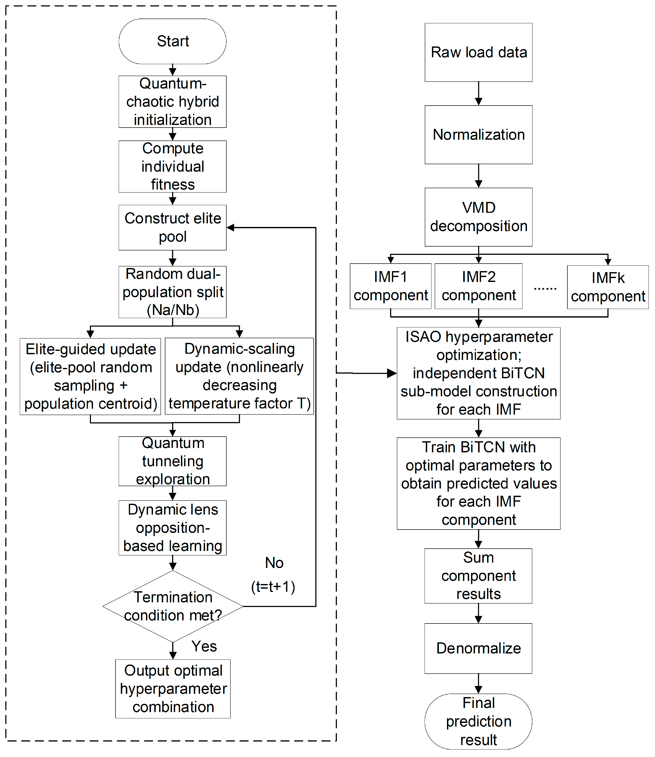
Building on the study of the ISAO algorithm and the VMD method, this paper establishes the ISAO-VMD-BiTCN combined prediction model. The model first applies VMD to decompose the original load data into multiple IMF components, then applies ISAO to optimize the BiTCN hyperparameters for each component, and finally aggregates and denormalizes the component-wise predictions to obtain the final forecast. The specific steps are as follows.

(1) Read the actual load data from the PJM electricity market and perform normalization preprocessing. The normalization expression is:

$$\tilde{x}={\displaystyle \frac{x-x_{min}}{x_{max}-x_{min}}}$$

(24)

where $\tilde{x}$ is the normalized data; x is the original data; and $x_{max}$ and $x_{min}$ are the maximum and minimum values of the data, respectively.

(2) Use VMD to decompose the normalized load sequence into K IMF components, reducing the nonlinearity and non-stationarity of the data and improving the predictability of each component.

(3) Construct a separate BiTCN prediction sub-model for each IMF component, and use ISAO to independently optimize the BiTCN network hyperparameters (number of convolution kernels NumFilters, convolution kernel size FilterSize, dropout rate, and learning rate LearnRate) for each component, obtaining the optimal hyperparameter combination for each.

(4) Train the BiTCN prediction model for each component using its optimal hyperparameters to obtain the predicted values for each IMF component. Superimpose the predicted values of all components and perform denormalization to obtain the final power load forecast.

The overall workflow of the proposed ISAO-VMD-BiTCN combined prediction model is shown in Figure 3.

6. Case Study Analysis

To validate the effectiveness of the ISAO-VMD-BiTCN model established in Section 5, this section conducts a case study using hourly power load data from the PJM electricity market from 1 July 2016 to 30 September 2016, comprising 2185 data points at a 1 h resolution. This summer period exhibits pronounced load fluctuations, substantial peak-valley differences, and strong nonlinearity, providing a challenging scenario for evaluating the forecasting accuracy and adaptability of the proposed model. All simulation experiments were carried out in the MATLAB 2024 environment.

6.1. Model Parameter Settings

Using the same VMD configuration adopted above, the normalized load data are decomposed into five IMF components. The resulting VMD decomposition results are shown in Figure 4. It should be noted that both the normalization and the VMD are applied to the entire load series prior to the subsequent train/test partitioning; because VMD jointly decomposes the whole signal, this introduces a mild form of information leakage from the test period into the preprocessing stage. The dataset is strictly partitioned into chronological sets: the first 80% is used for training and the remaining 20% for testing. During the optimization phase, 15% of the training data is used to calculate model fitness, ensuring the test set remains entirely unseen until final evaluation. The time-series sliding window length is set to 24 h with a prediction step of 1 h. The BiTCN hyperparameter search space is the number of convolution kernels NumFilters ∈ [16, 128], convolution kernel size FilterSize ∈ [2, 6], dropout rate ∈ [0, 0.4], and learning rate LearnRate ∈ [1 × 10⁻⁴, 5 × 10⁻³]. To improve the reliability of the comparative evaluation and assess the influence of stochasticity, all prediction models were independently evaluated using six random seeds. The results obtained from these independent runs were summarized using the mean. For all metaheuristic algorithms involved, the population size was set to 25, and the maximum number of iterations was set to 30.

6.2. Prediction Model Hyperparameter Optimization

The ISAO algorithm is used to independently optimize the BiTCN hyperparameters for each IMF component within the search space defined above. The final optimal hyperparameter configuration obtained for each component is shown in

Table 3. Optimal hyperparameter configuration for each IMF component.

Component	NumFilters	FilterSize	Dropout Rate	Initial Learning Rate	Validation-Set RMSE
IMF1	76	2	0.0000	1.00 × 10−4	0.0086
IMF2	41	2	0.0165	1.85 × 10−4	0.0241
IMF3	52	3	0.0513	1.28 × 10−3	0.0231
IMF4	80	5	0.2325	3.93 × 10−3	0.0221
IMF5	128	3	0.4000	2.88 × 10−3	0.0106

.

Analysis of Table 3 shows that the low-frequency components exhibit strong regularity, and ISAO selects a lower learning rate and a simpler network structure for them; the high-frequency components, in contrast, fluctuate drastically, and ISAO automatically assigns more convolution kernels and a higher dropout rate to suppress noise interference. This component-by-component, customized optimization strategy ensures—at the underlying architectural level—the overall prediction accuracy after subsequent superposition and reconstruction.

6.3. Data Comparison

To evaluate the forecasting performance of the proposed ISAO-VMD-BiTCN model, comparative experiments were conducted using the dataset described above, with LSTM, VMD-BiTCN, GWO-VMD-BiTCN, PSO-VMD-BiTCN, and SAO-VMD-BiTCN as comparison models.

To evaluate the performance of each prediction model, the evaluation is conducted from two complementary perspectives: predictive accuracy and statistical significance. Predictive accuracy is assessed using four quantitative metrics: Root Mean Square Error (RMSE), Mean Absolute Error (MAE), Mean Absolute Percentage Error (MAPE), and the Coefficient of Determination (R²). The experimental results obtained from six independent random seeds are summarized using the mean value to characterize the predictive performance of the model. Statistical significance is further assessed using the Diebold–Mariano (DM) test, which is performed separately for each random seed to examine whether the forecasting loss differences between ISAO-VMD-BiTCN and the competing models are statistically significant.

The specific results are reported in

Table 4. Comparison of prediction indicators across models.

Model	RMSE/MW	MAE/MW	MAPE/%	R2
LSTM	2679.14	2245.85	6.233	0.8932
VMD-BiTCN	2528.68	2055.16	5.748	0.9039
GWO-VMD-BiTCN	2355.84	1879.02	5.416	0.9168
PSO-VMD-BiTCN	2435.59	1949.81	5.529	0.9110
SAO-VMD-BiTCN	2342.23	1875.94	5.345	0.9180
ISAO-VMD-BiTCN	2202.14	1752.99	4.990	0.9272

, while the corresponding DM test results are presented in

Table 5. Diebold–Mariano test statistics and p-values.

Model	Statistic	S1	S2	S3	S4	S5	S6
LSTM	DM	3.5603	5.2404	1.2579	3.9585	2.4715	2.0651
	P	3.7042 × 10−4	1.6033 × 10−7	2.0843 × 10−1	7.5418 × 10−5	0.0135	0.0389
VMD-BiTCN	DM	6.2112	−1.5210	4.2664	3.1688	4.1802	2.8940
	P	5.2651 × 10−10	0.1283	1.9868 × 10−5	1.5307 × 10−3	2.9124 × 10−5	3.8043 × 10−3
GWO-VMD-BiTCN	DM	−1.3210	4.5843	4.6555	0.5226	2.4195	−1.4120
	P	0.1865	4.5543 × 10−6	3.2323 × 10−6	0.6013	0.0155	0.1579
PSO-VMD-BiTCN	DM	3.8687	4.1273	−1.7179	−1.3850	1.1582	6.3570
	P	1.0935 × 10−4	3.6698 × 10−5	0.8582	0.1661	0.2468	2.0560 × 10−10
SAO-VMD-BiTCN	DM	6.2156	−1.0455	−1.2140	3.3291	2.2418	−0.5695
	P	5.1128 × 10−10	0.2958	0.2248	8.7138 × 10−4	0.0249	0.5690

. Furthermore, Figure 5 and Figure 6 display the error-metric comparisons and actual-versus-predicted scatter plots, respectively.

As shown in Table 4, ISAO-VMD-BiTCN achieves the best mean predictive performance among the five comparison models. Based on the mean values, compared with the other prediction models, ISAO-VMD-BiTCN reduces RMSE by 17.80%, 12.91%, 6.52%, 9.58%, and 5.98%, respectively; reduces MAE by 21.94%, 14.70%, 6.71%, 10.09%, and 6.55%, respectively; reduces MAPE by 19.94%, 13.19%, 7.87%, 9.75%, and 6.64%, respectively; and improves R² by 3.81%, 2.58%, 1.13%, 1.78%, and 1.00%, respectively. These results indicate that the complete ISAO-VMD-BiTCN framework provides meaningful predictive improvements under the investigated experimental setting. However, the observed improvements cannot be attributed solely to the global search capability of ISAO, since differences in model structure, hyperparameter configuration, and training procedures may also contribute to the final forecasting performance. Figure 5 further visualizes the comparative performance, showing that ISAO-VMD-BiTCN has the lowest mean error levels and the highest mean R² among the compared models.

Figure 6 presents the actual-versus-predicted scatter plots for all models. The prediction points of ISAO-VMD-BiTCN are more closely distributed around the reference line than those of the competing models, indicating a stronger agreement between predicted and actual load values.

The Diebold–Mariano (DM) test results further assess whether the forecasting differences between ISAO-VMD-BiTCN and the competing models are statistically significant across different random initializations. Statistically significant favorable differences for ISAO-VMD-BiTCN are observed for 50–83.3% of the evaluated seeds across the competing models. According to the error-difference definition, $d_t=L\left(e_{other},t\right)-L\left(e_{ISAO},t\right)$. A positive DM statistic with $p<0.05$ indicates that the forecasting error of ISAO-VMD-BiTCN is significantly lower than that of the corresponding competing model. Although the statistical significance and direction of the differences are not consistent across every random seed, the DM results provide additional statistical evidence of favorable forecasting performance across multiple random initializations.

It should be noted that the present study has three main scope limitations. First, this study evaluates only a single summer season, July–September 2016, from the PJM market. Without coverage of other seasons or multiple years, this case study does not establish cross-seasonal or multi-year generalization. Second, electricity load is also influenced by exogenous factors beyond historical load patterns: temperature and humidity affect heating and cooling demand, while weekday type, weekends, and holidays alter electricity consumption patterns due to differences in human activity and operational schedules; seasonal changes in these factors may therefore contribute to variations in electricity demand and provide additional information for load forecasting [21]. However, the present study adopts a univariate forecasting setting and uses only historical load observations, so these exogenous variables are not explicitly modeled; accordingly, the proposed model should be interpreted as a load-history-based forecasting approach validated within the investigated single-season setting, rather than as a general-purpose, cross-seasonal forecasting model. Third, normalization and VMD are applied to the entire load series prior to the chronological train/test split; because VMD jointly decomposes the whole signal via ADMM, this introduces a mild form of information leakage from the test period into the preprocessing stage. This leakage is confined to an unsupervised, label-free preprocessing step rather than the supervised training loss itself, but a strictly causal or online decomposition scheme applied separately to the training and test partitions would eliminate this concern and is left for future work.

7. Conclusions

To address the nonlinear and nonstationary characteristics of power load data and the difficulty of determining BiTCN network hyperparameters, this study develops the ISAO and applies it to the hyperparameter optimization of a VMD-BiTCN forecasting framework. The ISAO incorporates four coordinated improvement strategies: quantum-chaotic hybrid initialization, elite-pool-guided dual-population updating, the quantum tunneling effect, and dynamic lens opposition-based learning. VMD is used to decompose the original load sequence into multiple IMF components, while ISAO independently optimizes the BiTCN hyperparameters for each component. On the CEC2022 benchmark suite, ISAO achieves the best mean and median performance on six of the 12 test functions and shows competitive performance against RIME, HBA, ARO, and SAO, with statistically significant differences observed on a substantial proportion of functions according to the Wilcoxon rank-sum test. On the PJM hourly load dataset, ISAO-VMD-BiTCN achieves the lowest RMSE, MAE, and MAPE and the highest R² among the compared models, with a 5.98% reduction in RMSE relative to SAO-VMD-BiTCN. The DM test based on six independent random seeds further indicates that ISAO-VMD-BiTCN exhibits statistically significant forecasting advantages under most random initializations, providing additional statistical support for its favorable forecasting performance, although the statistical significance and direction of the differences vary across random seeds.

These findings are naturally bounded by the single-season, univariate scope of the present evaluation, which motivates the following directions for future work. Future work will extend the evaluation to multiple seasons and years, incorporate relevant meteorological and calendar variables into a multivariate forecasting framework, and further investigate computational efficiency and real-time deployment.