DGPRT-ResNet: A Difference-Guided and Prototype-Regularized Residual Network with Trend Reconstruction for Small-Sample Hyperspectral Soil Total Nitrogen Prediction

Abstract

Accurate and rapid estimation of soil total nitrogen (TN) from visible–near-infrared hyperspectral data is important for precision agriculture, but small-sample modeling remains challenging because limited labeled samples often lead to unstable feature representations and insufficient use of local spectral variations. This study proposes DGPRT-ResNet, a difference-guided and prototype-regularized residual network with trend reconstruction, for small-sample hyperspectral soil TN prediction. A 2000-sample subset was constructed from the LUCAS 2009 soil spectral library. The spectra were preprocessed using multiplicative scatter correction and first-order derivative transformation, and piecewise pooling averaging was used to obtain 128-dimensional input representations. Based on a one-dimensional residual backbone, the proposed model integrates difference-guided residual calibration to enhance local spectral-shape variations, a prototype-regularized regression head to constrain the deep embedding distribution, and a segmental trend reconstruction auxiliary branch to preserve global spectral trends. Experimental results showed that DGPRT-ResNet achieved an R² of 0.926 and an RMSE of 0.985 g/kg on the test set, outperforming the baseline ResNet and its ablated variants. These results indicate that combining local difference modeling, feature-space regularization, and trend-preserving auxiliary supervision can improve the prediction accuracy of hyperspectral regression for soil TN estimation under the evaluated limited-sample setting.

1. Introduction

Soil total nitrogen (TN) is one of the most important indicators for evaluating soil fertility, nitrogen supply capacity, and nutrient cycling in agroecosystems. Accurate TN information is essential for precision fertilization, cropland quality assessment, and sustainable agricultural management. Traditional laboratory-based chemical methods can provide reliable measurements, but they are usually time-consuming, labor-intensive, and unsuitable for rapid monitoring over large areas. Therefore, developing fast, non-destructive, and cost-effective techniques for soil TN estimation has become an important topic in agricultural sensing and intelligent soil information acquisition.

Visible–near-infrared (Vis–NIR) hyperspectral spectroscopy provides a promising solution for rapid soil property estimation because it can capture continuous spectral responses related to soil organic matter, moisture, texture, and nutrient composition [1,2]. In recent years, Vis–NIR spectroscopy combined with machine learning has been widely used for predicting soil organic carbon, TN, pH, and other physicochemical properties [3,4]. Traditional chemometric and machine learning methods, such as partial least squares regression, support vector machines, random forests, and Cubist models, have achieved encouraging results in soil spectral modeling [5,6]. In particular, large-scale public soil spectral libraries, such as the LUCAS topsoil database, provide a valuable basis for developing and evaluating data-driven soil prediction models [7]. However, soil hyperspectral data usually contain high-dimensional, highly correlated, and noisy spectral bands. Scattering effects, baseline drift, sample heterogeneity, and local spectral fluctuations may weaken the effective relationship between spectral features and TN content, making accurate prediction still challenging.

With the development of deep learning, convolutional neural networks and residual networks have been increasingly introduced into spectral regression tasks. Compared with traditional methods, deep neural networks can automatically learn hierarchical and nonlinear feature representations from spectral sequences. Residual networks further improve deep feature extraction by using shortcut connections to ease optimization and reduce information loss in deep architectures [8]. These advantages make residual learning suitable for one-dimensional hyperspectral modeling. Nevertheless, deep models often rely on sufficient training samples. When only limited labeled soil samples are available, the model may suffer from unstable feature representation, overfitting, and poor generalization. This problem is particularly evident in soil TN prediction, where the spectral response of nitrogen is often indirect and affected by multiple soil background factors.

Small-sample hyperspectral regression has therefore become a key issue that needs further investigation. Existing studies have improved soil spectral regression through spectral preprocessing, informative-band selection, deep convolutional modeling, attention mechanisms, and compact network design. However, under limited-sample conditions, explicit modeling of local spectral variations, structural constraints on deep embeddings, and preservation of global spectral trends remain insufficiently explored. First, many models do not explicitly use local spectral difference information, although adjacent-band variations can reflect important changes in spectral shape. Second, the deep embeddings learned from limited samples may be scattered and weakly structured, which reduces regression stability. Third, models trained under small-sample conditions may focus excessively on local numerical patterns while ignoring the global spectral trend. Although prototype-based representation learning has shown effectiveness in limited-data scenarios by constraining samples around representative prototypes [9], its potential for continuous soil hyperspectral regression has not been sufficiently explored. Similarly, auxiliary supervision can provide additional constraints for feature learning, but how to design a trend-preserving auxiliary task suitable for soil spectral sequences remains an open problem.

Recent studies in related representation-learning tasks have also highlighted the value of explicitly modeling local structural variations and complementary frequency information. For example, band-mixed edge-aware interaction learning has been introduced to strengthen edge-sensitive and cross-modal feature interaction in RGB-T camouflaged object detection [10]. Multi-frequency perception with complementary fusion has also been explored to jointly exploit information at different frequency levels for complex-scene segmentation [11]. Although these studies address different vision tasks rather than soil hyperspectral regression, they suggest that explicitly incorporating local structural changes and complementary representation cues can provide useful inductive constraints for deep feature learning. These observations are conceptually related to the local difference modeling and trend-preserving mechanisms adopted in the present study.

To address these issues, this study proposes DGPRT-ResNet, a difference-guided and prototype-regularized residual network with trend reconstruction for small-sample hyperspectral soil TN prediction. The model is built on a one-dimensional residual backbone and integrates three task-oriented components. First, a difference-guided residual calibration module is introduced to enhance the modeling of local spectral-shape variations by using adjacent-band difference responses. Second, a prototype-regularized regression head is designed to constrain the deep embedding space and improve feature compactness under limited sample conditions. Third, a segmental trend reconstruction auxiliary branch is constructed to preserve global spectral trends and reduce overfitting to local fluctuations. In addition, multiplicative scatter correction and first-order derivative transformation are used to improve spectral quality, and piecewise pooling averaging is applied to obtain compact 128-dimensional input representations.

The main contributions of this study are summarized as follows. First, a difference-guided residual calibration mechanism is developed to strengthen local spectral variation modeling in small-sample soil hyperspectral regression. Second, a prototype-regularized regression strategy is introduced to improve the structure and stability of deep feature representations. Third, a segmental trend reconstruction auxiliary task is designed to guide the network to maintain global spectral-shape information. Finally, experiments on a 2000-sample subset constructed from the LUCAS 2009 soil spectral library [7] demonstrate that the proposed DGPRT-ResNet achieves better prediction performance than the baseline ResNet and its ablated variants, with an R² of 0.926 and an RMSE of 0.985 g/kg on the test set. These results suggest that combining local difference modeling, feature-space regularization, and trend-preserving auxiliary supervision can improve soil TN prediction under the evaluated limited-sample setting.

2. Materials and Methods

2.1. Dataset Introduction

The experimental data used in this study were obtained from the LUCAS-Topsoil 2009 soil spectral dataset [7]. The dataset was established within the framework of the Land Use/Cover Area Frame Survey (LUCAS) conducted by Eurostat and provides a large-scale topsoil database for European regions. Different from datasets collected from a single study area or a local experimental field, LUCAS-Topsoil 2009 contains soil samples from multiple countries and regions across Europe. Therefore, it has the characteristics of broad spatial coverage, diverse sample sources, and strong regional representativeness.

The LUCAS-Topsoil dataset contains both soil physicochemical properties and corresponding visible–near-infrared (Vis–NIR) spectral information. These data provide a reliable basis for constructing and evaluating data-driven soil property prediction models. In this study, soil total nitrogen (TN) was selected as the target variable, and the corresponding hyperspectral reflectance data were used as model inputs. TN is an important indicator of soil fertility and nitrogen supply capacity, and its rapid estimation is meaningful for precision agriculture and soil nutrient management.

For hyperspectral soil TN prediction, the LUCAS-Topsoil 2009 dataset is suitable for two main reasons. First, it is a publicly available dataset constructed under a relatively standardized survey and sampling framework, which helps improve the reproducibility and comparability of the study. Second, its multi-regional and multi-source topsoil samples provide diverse spectral and soil-property information, offering a representative basis for controlled within-dataset model evaluation. Based on this dataset, this study further constructed a small-sample experimental scenario to investigate the performance of the proposed DGPRT-ResNet model under limited training samples. It should be noted that the present evaluation is restricted to a soil TN subset derived from the LUCAS 2009 database and therefore does not constitute external validation across independent datasets or different soil properties.

2.2. Data Processing and Dataset Partitioning

To improve the modeling efficiency of Vis–NIR hyperspectral data and reduce the redundancy caused by strong correlations among adjacent spectral bands, the spectral inputs were compressed before model training. In this study, piecewise pooling averaging (PPA) was adopted to obtain a compact spectral representation. Specifically, each continuous spectrum was divided into a series of adjacent and non-overlapping intervals along the spectral dimension, and the reflectance values within each interval were averaged to form a lower-dimensional feature representation. This downsampling-based compression strategy can effectively reduce input dimensionality and computational cost while preserving the overall spectral trend and local absorption-related information. Therefore, PPA provides a practical balance between modeling efficiency and spectral information retention in soil property prediction tasks.

In addition, soil total nitrogen is a continuous regression target with an imbalanced distribution, and direct random splitting may lead to inconsistent label distributions between the training and test sets. To reduce the influence of accidental sample partitioning on model evaluation, a stratified random sampling strategy based on percentile binning was used for dataset partitioning. The continuous TN labels were first divided into multiple strata according to percentile thresholds, and samples within each stratum were then randomly assigned to the training and test sets at a fixed proportion. This strategy helps maintain similar label distributions between the two subsets, thereby improving evaluation fairness and reducing performance fluctuations caused by random splits. A fixed random seed was also used during partitioning to ensure the reproducibility of the experimental results.

2.2.1. Data Representation and Notation

Let the preprocessed dataset be denoted as

$$\mathcal{D}={\left(X_i,y_i\right)}_{i=1}^N.$$

where $N$ is the number of samples, $X_i$ represents the spectral feature vector of the $i$-th soil sample, and $y_i\in R$ denotes the corresponding soil total nitrogen content, which is treated as a continuous regression target.

After PPA-based dimensionality reduction, the spectral input of each sample is uniformly represented as a 128-dimensional feature vector:

$$X_i={\left[x_{i,1},x_{i,2},\dots ,x_{i,128}\right]}^{\mathrm{\top }}\in R^{128}.$$

where $x_{i,j}$ denotes the compressed spectral feature value of the $i$-th sample at the $j$-th segment. To match the input format of a one-dimensional convolutional network, each spectral vector is further reshaped by adding a single-channel dimension: $\widetilde{X_i}\in R^{1\times 128}$.

During mini-batch training, given a batch size $\mathrm{B}$, the model input tensor and the corresponding label vector are written as $X\in R^{B\times 1\times 128}, Y\in R^{B\times 1}$.

These notational conventions are used throughout the following descriptions of the proposed network architecture, module design, and training procedure, ensuring consistency between the mathematical formulation and model implementation.

2.2.2. Spectral Preprocessing and PPA Dimensionality Reduction

Vis–NIR hyperspectral reflectance spectra usually exhibit strong redundancy and high inter-band correlation along the spectral dimension. They are also susceptible to spectroscopic artifacts, such as scattering effects, baseline drift, and local random noise. Therefore, appropriate spectral preprocessing and feature compression before model training are important for improving modeling efficiency, training stability, and prediction robustness. In this study, multiplicative scatter correction (MSC) [12] and first-order derivative transformation (FD) [13] were first applied as a unified preprocessing procedure. MSC was used to reduce scattering variations caused by differences in soil particle size, surface roughness, and measurement conditions, while FD was used to enhance local spectral-shape variations and suppress baseline drift. Since the focus of this study is the proposed small-sample regression model rather than preprocessing optimization, the same MSC + FD preprocessing procedure was applied to all compared models to ensure fair comparison.

After preprocessing, piecewise pooling averaging (PPA) was used to reduce the dimensionality of the continuous spectra. PPA can be regarded as a band-averaging operation along the spectral axis. It reduces the input dimension by replacing dense spectral measurements within local intervals with their mean values. This strategy can effectively reduce computational cost and alleviate the adverse effects of multicollinearity and noise accumulation while preserving the overall spectral trend and the main absorption-related structural information.

Let the preprocessed spectral matrix be denoted as

$$A\in R^{m\times n}.$$

where $m$ is the number of samples and $n$ is the number of original spectral bands after preprocessing. PPA sequentially partitions the spectral dimension into $b$ adjacent and non-overlapping intervals. In this study, $b=128$ was used to construct a unified 128-dimensional spectral representation. The interval width is defined as $\mathrm{s}=⌊{\displaystyle \frac{n}{b}}⌋$.

For the $i$-th interval $\left(i=\mathrm{1,2},\dots ,b\right)$, the compressed feature of the $j$-th sample is calculated by averaging the spectral values within the corresponding interval:

$$A^{\prime }\left[:,i\right]={\displaystyle \frac{1}{s}}\sum _{k=1}^{s}A\left[:,\left(i-1\right)s+k\right]$$

(1)

After applying PPA to all samples, the reduced spectral feature matrix is obtained as $A^{\prime }\in R^{m\times b}$.

Since $b=128$ in this study, each soil sample is finally represented by a 128-dimensional spectral vector. Compared with directly using the original high-dimensional spectra, the compressed representation substantially reduces input dimensionality and computational burden while smoothing local random perturbations. Meanwhile, because PPA operates on consecutive spectral intervals, the compressed features can still preserve the global spectral trend and the main band-position structure. During network training and inference, these fixed-length 128-dimensional spectral vectors are directly used as model inputs, ensuring consistent input dimensionality and improving training efficiency and reproducibility.

2.2.3. Continuous-Label Stratification via Percentile Binning

Because soil total nitrogen $Y$ is a continuous regression variable, its distribution is often skewed, long-tailed, or imbalanced with respect to extreme-value samples. If the training and test sets are generated by fully random splitting, the proportions of samples in high-value or low-value ranges may differ substantially between the two subsets. Such distribution inconsistency can introduce evaluation bias and reduce the comparability of model conclusions. Therefore, this study adopted a percentile-binning strategy to map continuous TN labels into discrete stratification indices, followed by stratified random sampling to keep the label distributions of the training and test sets as consistent as possible.

Specifically, let the number of strata be $K$. The bin-boundary vector is constructed according to the percentiles of the continuous label set $Y$:

$$\beta =\left\{{\beta }_0,{\beta }_1,\dots ,{\beta }_K\right\}, {\beta }_j=Percentile\left(Y,{\displaystyle \frac{100j}{K}}\right), j=\mathrm{0,1},\dots ,K$$

(2)

In this study, $K=50$, corresponding to percentile intervals of approximately 2%. Each continuous label $y_i$ is then mapped to a discrete stratum index $C_i$ according to the interval in which it falls:

$$C_i=j ⟺ y_i\in \left[{\beta }_j,{\beta }_{j+1}\right), C_i\in \mathrm{0,1},2,\dots ,K-1$$

(3)

For the last interval, the upper boundary is included to ensure that the maximum label value is assigned to a valid stratum. To improve the robustness of stratification, boundary inclusion and duplicate percentile values are handled consistently. When many samples share identical TN values, adjacent percentile boundaries may coincide. In such cases, coincident boundaries are merged or treated as equivalent to ensure that the resulting strata remain valid and stable.

Based on the discrete stratification labels $C_i$, the subsequent train/test split randomly samples a fixed proportion of data within each stratum. This process helps maintain the overall TN label distribution between the training and test sets, thereby improving the fairness and reproducibility of model evaluation.

2.2.4. Stratified Random Sampling for Training and Test-Set Partitioning

After obtaining the discrete stratification labels $\left\{C_i{\}}_{i=1}^N\right.$, the samples were partitioned into training and test sets under stratification constraints. Let $r$ denote the test-set ratio. The training set ${\mathcal{D}}_{\mathit{train}}$ and test set ${\mathcal{D}}_{\mathit{test}}$ satisfy the following conditions:

$${\mathcal{D}}_{\mathit{train}}\cup {\mathcal{D}}_{\mathit{test}}=\mathcal{D}, {\mathcal{D}}_{\mathit{train}}\cap {\mathcal{D}}_{\mathit{test}}=\varnothing , \left|{\mathcal{D}}_{\mathit{test}}\right|\approx rN$$

(4)

In this study, $r=0.3$, corresponding to a 7:3 split between the training and test sets. Specifically, within each stratum, the samples were randomly shuffled while preserving the correspondence between spectral features and TN labels. Then, approximately 30% of the samples in each stratum were assigned to the test set, and the remaining samples were assigned to the training set. Therefore, the final dataset contained 1400 training samples and 600 test samples.

Unlike fully random splitting, the proposed stratified partitioning strategy imposes label-distribution constraints during sampling. That is, the test samples are selected proportionally from each TN label stratum, rather than from the entire dataset without considering label distribution. This procedure helps maintain similar TN distributions between the training and test sets, especially in high-value and low-value ranges. As a result, the evaluation results are less affected by accidental sample splitting and are more suitable for fair comparison among different models.

To ensure reproducibility, a fixed random seed was used during the partitioning process. Under the same parameter settings, the same training and test subsets can be obtained. The resulting ${\mathcal{D}}_{\mathit{train}}$ and ${\mathcal{D}}_{\mathit{test}}$ were then used for tensor construction, mini-batch loading, model training, and final performance evaluation.

2.3. Proposed Modeling Method

2.3.1. Overall Architecture of DGPRT-ResNet

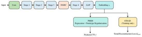
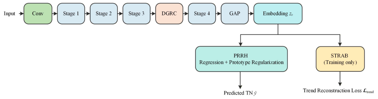
The overall workflow of the proposed DGPRT-ResNet is shown in Figure 1. The model takes the preprocessed and dimension-reduced soil hyperspectral sequence as input. In this study, each input sample is represented as a one-dimensional spectral vector with a size of $1\times 128$. The input first passes through an initial convolutional layer, which performs shallow feature mapping and transforms the compact spectral vector into a higher-dimensional feature representation suitable for residual feature extraction.

Figure 1. Overall architecture and information flow of DGPRT-ResNet. DGRC is inserted between Stage 3 and Stage 4; PRRH and STRAB share the embedding feature after GAP, and STRAB is used only during training.

After the initial convolution, the features are sequentially processed by four residual stages, denoted as Stage 1 to Stage 4. These stages gradually extract hierarchical spectral representations, from shallow local spectral patterns to deeper abstract features. The residual learning framework allows spectral information to be propagated across layers through shortcut connections, which helps alleviate gradient degradation and feature loss during deep network training.

To enhance the model’s sensitivity to local spectral-shape variations, a Difference-Guided Residual Calibration (DGRC) module is inserted between Stage 3 and Stage 4. This module uses local difference responses along the spectral dimension to recalibrate residual features, thereby strengthening the representation of spectral inflection, local fluctuation, and fine-grained band information. The detailed design of DGRC is described in Section 2.3.2.

After Stage 4, global average pooling (GAP) is applied to compress the high-level feature maps into a global feature vector, which is subsequently mapped to the embedding vector $z$. The embedding vector is fed into the PRRH regression head to produce the predicted TN value. During training, the same embedding vector is also provided to STRAB for auxiliary trend reconstruction. STRAB is used only to construct the auxiliary loss and is removed during inference. More specifically, the 128-dimensional input spectrum is sequentially processed by the initial convolution and four residual stages. DGRC is inserted after Stage 3 and before Stage 4 to recalibrate the intermediate residual representation. After Stage 4, GAP produces a global feature vector that is further mapped into the embedding space. The same embedding is shared by PRRH and STRAB: PRRH produces the final continuous TN prediction and imposes prototype-based regularization during training, whereas STRAB provides auxiliary trend supervision only during training. Therefore, the three components interact through a shared sequential feature representation rather than operating as independent prediction branches.

Overall, DGPRT-ResNet is constructed around three key ideas: local difference-aware feature calibration, prototype-regularized regression, and trend-preserving auxiliary supervision. The complete architecture enables the model to extract discriminative spectral features while maintaining feature compactness and spectral trend consistency, which is particularly beneficial for small-sample hyperspectral soil total nitrogen prediction.

2.3.2. Difference-Guided Residual Calibration

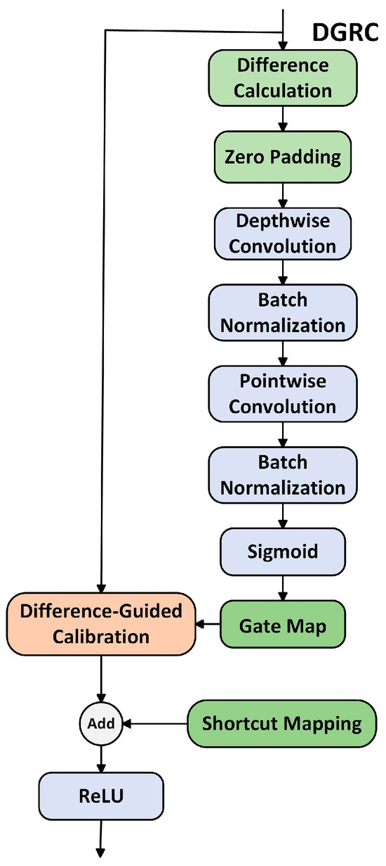
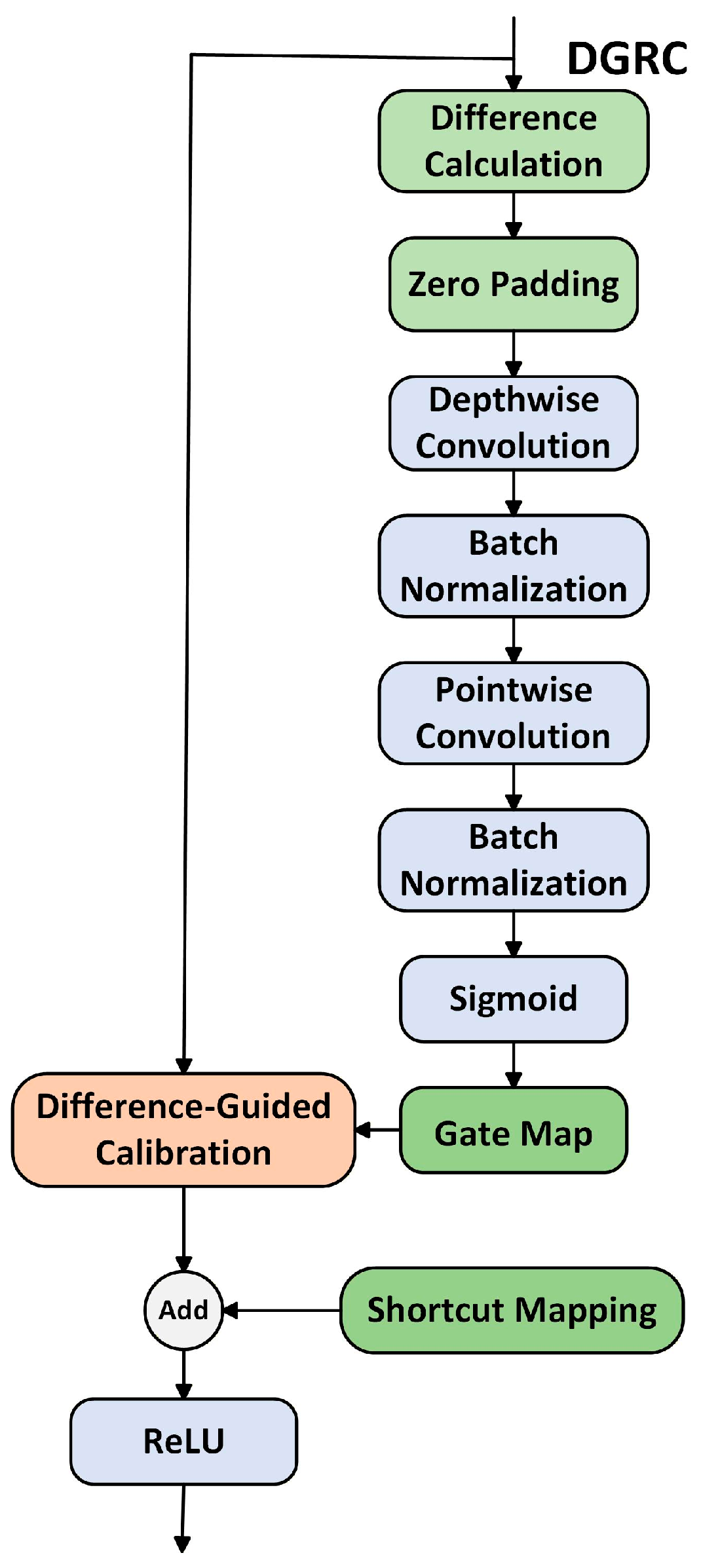
The structure of the DGRC module is shown in Figure 2. As illustrated in the DGRC schematic, the proposed DGPRT-ResNet introduces a Difference-Guided Residual Calibration (DGRC) module into the deep feature extraction stage. In this study, DGRC is inserted between Stage 3 and Stage 4 to recalibrate the residual features before they are fused with the shortcut branch. The purpose of this design is to address the limited utilization of local spectral-shape variations, the weak sensitivity to low-response but informative bands, and the insufficient attention to key spectral inflection patterns in small-sample soil hyperspectral modeling. Instead of directly feeding the residual feature into residual addition after conventional convolutional transformation, DGRC first explicitly characterizes local difference responses along the spectral dimension and then adaptively modulates the residual feature according to the difference intensity. In this way, the model can better perceive local spectral variations, peak–valley transitions, and fine-grained band differences.

Figure 2. Structure and residual information flow of the DGRC module.

Let the output feature of the residual main branch after convolution, normalization, and activation be denoted as

$$Z\in R^{B\times C\times L}$$

where $B$ is the batch size, $C$ is the number of channels, and $L$ is the spectral feature length. Since the discriminative information in soil hyperspectral sequences is more strongly reflected by local spectral-shape changes than by isolated single-point responses, DGRC first constructs a difference response map along the spectral dimension:

$$D=Pad\left(\left|Z_{:,:,2:L}-Z_{:,:,1:L-1}\right|\right)$$

(5)

where $\left|\cdot \right|$ denotes the absolute-value operation, and $Pad\left(·\right)$ restores the difference feature to the same length as the original feature by boundary padding. Equation (5) explicitly depicts the intensity of local spectral-shape variation, enabling the network to focus more on spectral regions with stronger local changes.

After obtaining the difference response map, DGRC further constructs a difference-guided gate to jointly model local difference patterns and channel interactions. The process can be written as

$$G=\sigma \left({BN}_p\left({Conv}_p\left({BN}_d\left({Conv}_d\left(D\right)\right)\right)\right)\right)$$

(6)

where ${Conv}_d\left(\cdot \right)$ denotes one-dimensional depthwise convolution, which is used to extract local difference patterns along the spectral axis within each channel; ${Conv}_p\left(\cdot \right)$ denotes pointwise convolution, which is used to fuse channel-wise information; ${BN}_d\left(\cdot \right)$ and ${BN}_p\left(\cdot \right)$ denote batch normalization operations; and $\sigma \left(\cdot \right)$ denotes the Sigmoid activation function. The resulting gate $G\in R^{B\times C\times L}$ is a position-sensitive modulation map, which adaptively adjusts the feature responses across different channels and spectral locations. In implementation, this process corresponds to the “difference computation → padding → depthwise convolution → batch normalization → pointwise convolution → batch normalization → Sigmoid” path shown in the DGRC schematic.

At the calibration stage, DGRC adopts a “retain original residual response + difference-guided enhancement” strategy, rather than directly suppressing or shrinking the residual feature. The calibrated residual feature and the block output are defined as

$$\tilde{Z}=Z\odot \left(1+G\right),H\left(X\right)=ReLU\left(\tilde{Z}+S\left(X\right)\right)$$

(7)

where $\odot$ denotes element-wise multiplication, $\mathrm{X}$ is the input of the residual block, and $S\left(X\right)$ denotes the shortcut mapping. When the input and output dimensions are identical, $S\left(X\right)=X$; otherwise, $S\left(X\right)$ is implemented by a linear projection for dimension alignment. As shown in Equation (7), DGRC enhances the residual feature through the difference-guided gate before residual addition, thereby highlighting local spectral variations that are more relevant to the target variable while preserving the original representational capacity of the residual branch.

Overall, DGRC explicitly incorporates local difference responses into the residual calibration process and unifies “difference extraction–feature enhancement” within a residual learning framework. Compared with directly stacking convolutional layers to learn spectral patterns automatically, this mechanism can more effectively emphasize informative local variations under small-sample conditions. As a result, it provides more discriminative deep spectral representations for the subsequent prototype-regularized regression head and the segmental trend auxiliary branch. Unlike the first-order derivative used in spectral preprocessing, DGRC operates on learned intermediate feature maps and transforms local difference responses into a trainable gating signal for residual recalibration. Therefore, DGRC performs feature-dependent deep calibration rather than simply repeating derivative preprocessing.

2.3.3. Prototype-Regularized Regression Head

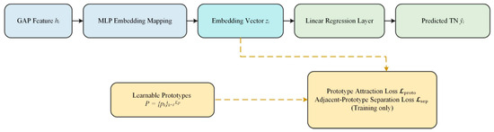
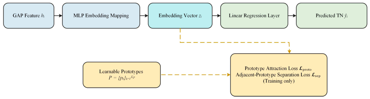
The structure of the Prototype-Regularized Regression Head (PRRH) is shown in Figure 3. It consists of an MLP-based embedding mapping, a prototype regularization mechanism, and a final prediction layer. After the deep feature extraction of the residual backbone and global average pooling (GAP), DGPRT-ResNet employs a Prototype-Regularized Regression Head (PRRH) in the main regression branch. The PRRH is designed to complete soil total nitrogen prediction while imposing structural constraints on the deep feature space. Its main purpose is to alleviate feature dispersion under small-sample conditions and encourage samples with similar TN values to form compact and well-separated clusters in the embedding space.

Figure 3. Structure of PRRH, including continuous TN regression and prototype-based embedding regularization. Yellow dashed arrows indicate the training-only paths used to calculate the prototype attraction loss and the adjacent-prototype separation loss.

Let the deep feature representation of the $i$-th sample after GAP and embedding mapping be denoted as

$$z_i\in R^d,\hspace{1em}i=\mathrm{1,2},\dots ,N$$

(8)

where $d$ denotes the embedding dimension and $N$ is the number of training samples. Based on this feature representation, the main regression branch outputs the predicted soil total nitrogen value through a linear regression layer:

$$\widehat{y_i}=W_r{z}_i+b_r$$

(9)

where $W_r$ and $b_r$ denote the weight matrix and bias term of the regression layer, respectively, and $\widehat{y_i}$ is the predicted TN value of sample $i$. The regression prediction is directly produced from the embedding vector, whereas prototype regularization is imposed as an auxiliary constraint on the embedding space during training, indicating that PRRH is not an independent auxiliary module but a core component directly serving continuous-value regression.

To enhance the structure of the feature space, the training labels are divided into $K_p$ ordered intervals according to their numerical distribution, and each interval is assigned a learnable prototype vector. The prototype set is defined as

$$P=\left\{p_1,p_2,\dots ,p_{K_p}\right\}, p_k\in R^d$$

(10)

where $p_k$ denotes the prototype center corresponding to the $k$-th label interval. The prototype vectors are treated as trainable model parameters and are jointly optimized with the network parameters through back-propagation. During training, the prototype attraction and adjacent-prototype separation losses provide gradient signals for the prototype vectors, so that their positions in the embedding space are dynamically updated together with the backbone and regression head. For sample $i$, its interval index is denoted as $c_i$. To encourage samples to approach the prototype of their corresponding label interval, the prototype attraction loss is defined as

$${\mathcal{L}}_{proto}={\displaystyle \frac{1}{N}}{\displaystyle \sum _{i=1}^N}{‖z_i-p_{c_i}‖}_2^2$$

(11)

This loss term pulls the feature representation of each sample toward the prototype center of its label interval, thereby improving the compactness of features within the same interval. For small-sample hyperspectral regression, such a constraint helps reduce the instability caused by scattered deep features and limited training samples.

However, using only prototype attraction may cause prototypes from different label intervals to become too close to each other, which weakens the separability of the feature space. Therefore, an adjacent-prototype separation loss is introduced between adjacent prototypes:

$${\mathcal{L}}_{sep}={\displaystyle \frac{1}{K_p-1}}{\displaystyle \sum _{k=1}^{K_p-1}}max\left(0,\delta -{‖p_{k+1}-p_k‖}_2\right)$$

(12)

where $\delta$ denotes the minimum separation margin between adjacent prototypes. This term encourages prototypes corresponding to different label intervals to maintain a reasonable distance from each other. In other words, the prototype attraction loss emphasizes intra-interval compactness, while the adjacent-prototype separation loss enhances inter-interval separability. Together, they provide a structured constraint for the deep embedding space.

The main regression loss is defined using the mean squared error between predicted and true TN values:

$${\mathcal{L}}_{reg}={\displaystyle \frac{1}{N}}{\displaystyle \sum _{i=1}^N}{\left(\widehat{y_i}-y_i\right)}^2$$

(13)

Finally, the overall loss of PRRH is composed of the regression loss, prototype attraction loss, and adjacent-prototype separation loss:

$${\mathcal{L}}_{PRRH}={\mathcal{L}}_{reg}+{\lambda }_p{\mathcal{L}}_{proto}+{\lambda }_s{\mathcal{L}}_{sep}$$

(14)

where ${\lambda }_p$ and ${\lambda }_s$ are weighting coefficients controlling the contributions of the prototype attraction loss and adjacent-prototype separation loss, respectively. These coefficients were kept fixed throughout all reported DGPRT-ResNet experiments to maintain a consistent optimization configuration across the ablation and comparison settings. The present study focuses on evaluating the architectural contributions of the proposed modules rather than systematically optimizing these loss-weighting coefficients.

According to Equation (14), PRRH does not replace the regression task. Instead, it introduces structural constraints into the deep feature space on the basis of continuous-value prediction. Unlike prototype learning in classification, where each prototype normally represents a discrete semantic class, the ordered label intervals in PRRH are used only to construct geometric constraints in the embedding space. The final TN prediction remains continuous and is directly optimized by the regression loss. Therefore, the prototype mechanism does not convert the regression problem into a classification task; instead, it encourages samples with similar continuous TN values to form more compact feature distributions while maintaining reasonable separation between different label ranges. Overall, PRRH provides a structured embedding constraint for small-sample continuous regression. Unlike prototype learning in classification, the prototypes in PRRH are used only to organize samples with similar continuous TN values in the embedding space, while the final prediction remains a continuous regression value optimized by the regression loss.

2.3.4. Segmental Trend Reconstruction Auxiliary Branch

In addition to the main regression branch, DGPRT-ResNet introduces a Segmental Trend Reconstruction Auxiliary Branch (STRAB) during training. STRAB receives the embedding vector obtained after global average pooling and embedding mapping and predicts a compact segmental trend vector through a lightweight multilayer perceptron. This branch provides auxiliary supervision for the shared feature representation and does not directly produce the TN prediction. During inference, STRAB is removed and only the main regression branch is retained.

Let the input one-dimensional spectral feature be denoted as

$$X\in R^{B\times 1\times L}$$

where $B$ is the batch size and $L$ is the spectral length. In this study, after preprocessing and dimensionality reduction, the input spectral length is $L=128$. To extract representative trend supervision from the input spectrum, first-order and second-order differences are calculated along the spectral dimension. The first-order difference describes the local change tendency of the spectral curve, while the second-order difference reflects the local curvature or bending intensity.

The input spectrum is divided into $M$ continuous spectral segments. For the $m$-th segment, the first-order trend statistic and second-order curvature statistic are defined as

$$s_m=Mean\left(\mathsf{\Delta }{X}_m\right),c_m=Mean\left(\left|{\mathsf{\Delta }}^2{X}_m\right|\right)$$

(15)

where $\mathsf{\Delta }{X}_m$ denotes the first-order difference feature within the $m$-th segment, ${\mathsf{\Delta }}^2{X}_m$ denotes the corresponding second-order difference feature, and $Mean\left(\cdot \right)$ represents average pooling over all positions within the segment. In Equation (15), $s_m$ is used to describe the average variation trend of the segment, while $c_m$ reflects the average curvature intensity of the segment. By extracting these two types of statistics from all segments, the trend target vector of the input spectrum is constructed as

$$t=\left[s_1,c_1,s_2,c_2,\dots ,s_M,c_M\right]\in R^{2M}$$

(16)

At the network output stage, the deep embedding feature $z_i\in R^d$ obtained from the main network is used as the input of STRAB. A lightweight fully connected mapping is employed to generate the predicted trend vector:

$$\widehat{t_i}=F_{trend}\left(z_i\right)$$

(17)

where $F_{trend}\left(\cdot \right)$ denotes the nonlinear mapping function of the trend reconstruction branch, and ${\widehat{t}}_i$ is the predicted trend vector for the $i$-th sample. In implementation, as shown in Figure 4, STRAB follows a lightweight “Linear–ReLU–Linear–ReLU–Linear–Trend Prediction Vector” pathway. It should be noted that STRAB is not an independent prediction branch for soil total nitrogen. Instead, it serves as an auxiliary supervision branch acting on the deep representation learned by the main network.

Figure 4. Structure of STRAB for auxiliary trend supervision during training.

To ensure that the deep features preserve overall spectral trend information while maintaining regression discriminability, the segmental trend reconstruction loss is defined using the mean squared error:

$${\mathcal{L}}_{trend}={\displaystyle \frac{1}{N}}{\displaystyle \sum _{i=1}^N}{‖\widehat{t_i}-t_i‖}_2^2$$

(18)

The final optimization objective of DGPRT-ResNet combines the PRRH loss and the STRAB auxiliary loss:

$${\mathcal{L}}_{DGPRT}={\mathcal{L}}_{PRRH}{+\lambda }_t{\mathcal{L}}_{trend}$$

(19)

where ${\mathcal{L}}_{PRRH}$ denotes the loss of the prototype-regularized regression head, ${\mathcal{L}}_{trend}$ denotes the segmental trend reconstruction loss, and ${\lambda }_t$ controls the contribution of the trend-preserving auxiliary objective relative to the primary regression objective. The same fixed coefficient configuration was used throughout the reported experiments without model-specific adjustment. A systematic sensitivity analysis of this coefficient was not included in the present study.

The auxiliary target is derived directly from the same input spectrum used for TN regression and therefore does not require additional external labels. Because PRRH and STRAB share the same deep embedding, minimizing the trend reconstruction loss constrains this representation to retain segmental spectral-shape information while it is simultaneously optimized for the scalar TN regression objective. Thus, STRAB serves as a complementary representation constraint rather than an independent prediction task. Its contribution is also supported by the single-module ablation result in Table 1, where introducing STRAB alone improves the baseline prediction performance.

Table 1. Ablation results of DGPRT-ResNet.

Model	DGRC	PRRH	STRAB	R2	RMSE (g/kg)
Baseline ResNet	✗	✗	✗	0.898	1.152
Baseline + D	✓	✗	✗	0.907	1.096
Baseline + P	✗	✓	✗	0.908	1.094
Baseline + T	✗	✗	✓	0.911	1.078
Baseline + D + P	✓	✓	✗	0.916	1.045
DGPRT-ResNet	✓	✓	✓	0.926	0.985

Note: D denotes the Difference-Guided Residual Calibration module (DGRC), P denotes the Prototype-Regularized Regression Head (PRRH), and T denotes the Segmental Trend Reconstruction Auxiliary Branch (STRAB). A checkmark indicates that the corresponding module was included, whereas a cross indicates that it was excluded.

According to Equations (18) and (19), STRAB does not require the network to reconstruct the complete original spectrum. Instead, it only reconstructs a compact trend representation composed of first-order variation and second-order curvature statistics. This design avoids the additional parameter burden and redundant information interference caused by direct spectral reconstruction, while still guiding the model to preserve the overall spectral-shape structure related to soil total nitrogen. For small-sample regression, this auxiliary supervision helps prevent the model from relying excessively on local numerical patterns and reduces the risk of overfitting.

Overall, STRAB provides an additional constraint for DGPRT-ResNet from the perspective of global trend preservation. If DGRC mainly focuses on local difference responses and PRRH mainly focuses on the structure of the deep feature space, then STRAB further strengthens the model’s ability to represent the overall spectral trend of the input. The three components jointly enable DGPRT-ResNet to balance local spectral modeling, feature-space regularization, and global trend preservation, thereby improving the prediction performance of hyperspectral soil total nitrogen under small-sample conditions. STRAB does not reconstruct the original spectrum directly. Instead, it reconstructs compact segmental first- and second-order trend statistics to provide an auxiliary constraint on the shared embedding.

2.4. Model Evaluation

To comprehensively and objectively evaluate the regression performance of the proposed model for soil total nitrogen prediction, model assessment was conducted from two perspectives: quantitative evaluation metrics and visual diagnostic analysis. The quantitative metrics were used to measure the overall fitting ability and prediction error of each model, while the visual diagnostic analysis was used to further examine the consistency between predicted and observed values as well as the distribution of prediction residuals.

For a fair comparison, all models were trained and evaluated under the same dataset partition, preprocessing procedure, training settings, and evaluation metrics. During model training, the same checkpoint-saving strategy was adopted for all compared methods. The test set was used only for final performance evaluation and was not involved in model parameter optimization. In addition, prediction scatter plots and residual distribution plots were used to visually analyze the predictive behavior of the models, thereby providing a more intuitive understanding of model accuracy, prediction bias, and residual characteristics.

2.5. Evaluation Metrics

Let the test set contain $n$ samples. The ground-truth soil total nitrogen content and the corresponding model prediction of the $i$-th sample are denoted as $y_i$ and $\widehat{y_i}$, respectively. The mean value of the ground-truth TN values is calculated as

$$\overline{y}={\displaystyle \frac{1}{n}}{\sum }_{i=1}^n{y}_i$$

(20)

In this study, the coefficient of determination $\left(R^2\right)$ and root mean square error (RMSE) were used as the primary evaluation metrics. Specifically, $R^2$ measures the proportion of variance in the observed values that can be explained by the model. A value closer to 1 indicates better agreement between predictions and observations. RMSE reflects the overall magnitude of prediction errors, where a smaller value indicates higher prediction accuracy. The two metrics are defined as follows:

$$R^2=1-{\displaystyle \frac{{\sum }_{i=1}^n{\left(y_i-\widehat{y_i}\right)}^2}{{\sum }_{i=1}^n{\left(y_i-\overline{y}\right)}^2}}$$

(21)

$$\mathrm{RMSE}=\sqrt{{\displaystyle \frac{1}{n}}\sum _{i=1}^n{\left(y_i-\widehat{y_i}\right)}^2}$$

(22)

Since the soil total nitrogen values in the LUCAS dataset are expressed in g/kg, RMSE is also reported in g/kg. In the following experiments, a higher $R^2$ and a lower RMSE indicate better prediction performance [14,15].

2.6. Experimental Setup

The experiments were conducted on a workstation equipped with an AMD Ryzen 7 9700X processor (AMD, Santa Clara, CA, USA) and an NVIDIA GeForce RTX 4070 SUPER GPU (NVIDIA, Santa Clara, CA, USA). The software environment consisted of Windows 11 as the operating system, Python 3.9 as the programming language, and PyTorch 2.7.1 as the deep learning framework, compiled with CUDA 12.8 and cuDNN 9.7 support. CUDA acceleration was enabled during training. Under this configuration, the model training process was able to fully utilize GPU acceleration, ensuring efficient computation and stable memory usage throughout the experiments.

For all reported experiments, the same preprocessing procedure, data-partitioning protocol, checkpoint-selection strategy, and evaluation metrics were adopted to ensure a consistent comparison. The loss-weighting coefficients of DGPRT-ResNet were kept fixed throughout the experiments. The percentile-based stratified 7:3 training/test partition was generated using a fixed random seed, so that all compared models and ablation variants were evaluated under the same data-partitioning protocol. This fixed-setting design was intended to provide a reproducible and controlled comparison rather than to estimate variability across repeated independent runs. For the baseline models, their model-specific architectures were retained, while the input data, preprocessing procedure, training/test partition, checkpoint-selection rule, and evaluation procedure were kept consistent. No baseline model used additional training samples or a different test partition.

3. Results

To verify the effectiveness of DGPRT-ResNet in small-sample hyperspectral soil total nitrogen prediction, comparative experiments and ablation experiments were conducted under the same experimental settings. The performance of each model was evaluated using the coefficient of determination $\left(R^2\right)$ and root mean square error (RMSE). Specifically, $R^2$ was used to measure the fitting ability of the model to the variation pattern of soil total nitrogen, while RMSE was used to reflect the overall prediction error.

In addition to quantitative evaluation, prediction scatter plots and residual analysis were further used to examine the consistency between predicted and measured values. By comprehensively analyzing the results of different models and different module combinations, the performance advantages of DGPRT-ResNet under small-sample conditions and the contribution of each component can be more clearly demonstrated.

3.1. Ablation Experiment

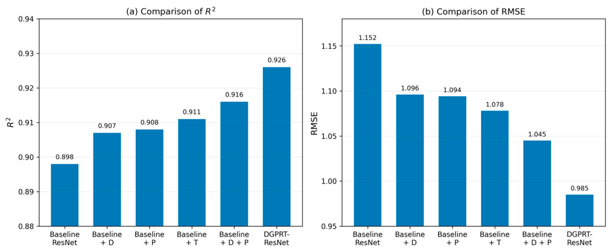
To further evaluate the contribution of each component in DGPRT-ResNet to small-sample hyperspectral soil total nitrogen prediction, ablation experiments were conducted based on the baseline ResNet. Specifically, the Difference-Guided Residual Calibration module (DGRC), Prototype-Regularized Regression Head (PRRH), and Segmental Trend Reconstruction Auxiliary Branch (STRAB) were introduced individually or in combination. The baseline ResNet was used as the unified reference model. The experimental results are shown in Table 1. To more intuitively compare the performance changes caused by different module combinations, the corresponding $R^2$ and RMSE results are further visualized in Figure 5.

Figure 5. Comparison of ablation results for different module combinations.

As shown in Table 1, all three proposed components improved the prediction performance when introduced individually. Compared with the baseline ResNet, introducing only DGRC increased $R^2$ from 0.898 to 0.907 and reduced RMSE from 1.152 to 1.096. This indicates that DGRC can enhance the model’s ability to capture local spectral-shape variations and key band transition information. When only PRRH was introduced, $R^2$ increased to 0.908 and RMSE decreased to 1.094, suggesting that prototype regularization helps alleviate the dispersion of deep features under small-sample conditions and improves regression performance under the evaluated setting. Among the single-module variants, the model with only STRAB achieved the best performance, with $R^2=0.911$ and RMSE = 1.078. This result indicates that trend auxiliary supervision can effectively enhance the model’s ability to preserve the overall spectral-shape pattern.

For the dual-module setting, the simultaneous introduction of DGRC and PRRH further improved the model performance, achieving an $R^2$ of 0.916 and an RMSE of 1.045. This result shows that local difference enhancement and feature-space regularization are complementary. On this basis, when STRAB was further added, the complete DGPRT-ResNet achieved the best performance, with $R^2=0.926$ and RMSE = 0.985. Compared with the baseline ResNet, the complete model improved $R^2$ by 0.028 and reduced RMSE by 0.167. Compared with Baseline + D + P, the addition of STRAB further improved $R^2$ by 0.010 and reduced RMSE by 0.060.

The current ablation design includes the baseline model, all three single-module variants, one representative dual-module configuration, and the complete three-module model. This setting enables the individual contribution of DGRC, PRRH, and STRAB to be directly examined, while also showing the incremental effect of introducing STRAB after DGRC and PRRH. Other possible dual-module combinations were not exhaustively evaluated in the present study.

Figure 5 further illustrates the performance trends of different module combinations. With the gradual introduction of DGRC, PRRH, and STRAB, $R^2$ shows a stable increasing trend, while RMSE continuously decreases. The single-module variants all outperform the baseline ResNet, the dual-module variant performs better than the single-module variants, and the complete DGPRT-ResNet achieves the best overall result. These findings confirm that the performance improvement of DGPRT-ResNet does not rely on a single component, but results from the collaborative effects of local difference modeling, feature-space regularization, and global trend preservation.

The ablation results provide indirect evidence for the different roles of the three components. The improvement obtained by DGRC suggests that difference-aware residual recalibration provides useful information beyond the baseline residual representation. The improvement obtained by PRRH indicates that structural constraints on the embedding space are beneficial under limited samples. Among the single-module variants, STRAB provides the largest improvement, suggesting that preserving segmental spectral trends provides a complementary constraint to the scalar TN regression objective. Direct visualization of intermediate feature maps or embedding distributions was not performed in the present study.

Overall, DGRC, PRRH, and STRAB improve model performance from three complementary perspectives. DGRC mainly addresses the insufficient utilization of local spectral-shape variations under small-sample conditions; PRRH improves the compactness and separability of deep feature representations; and STRAB strengthens the preservation of global spectral trend information. Their joint use enables DGPRT-ResNet to achieve higher prediction accuracy and lower prediction error under the evaluated small-sample setting.

3.2. Prediction Result Analysis

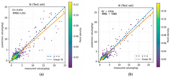
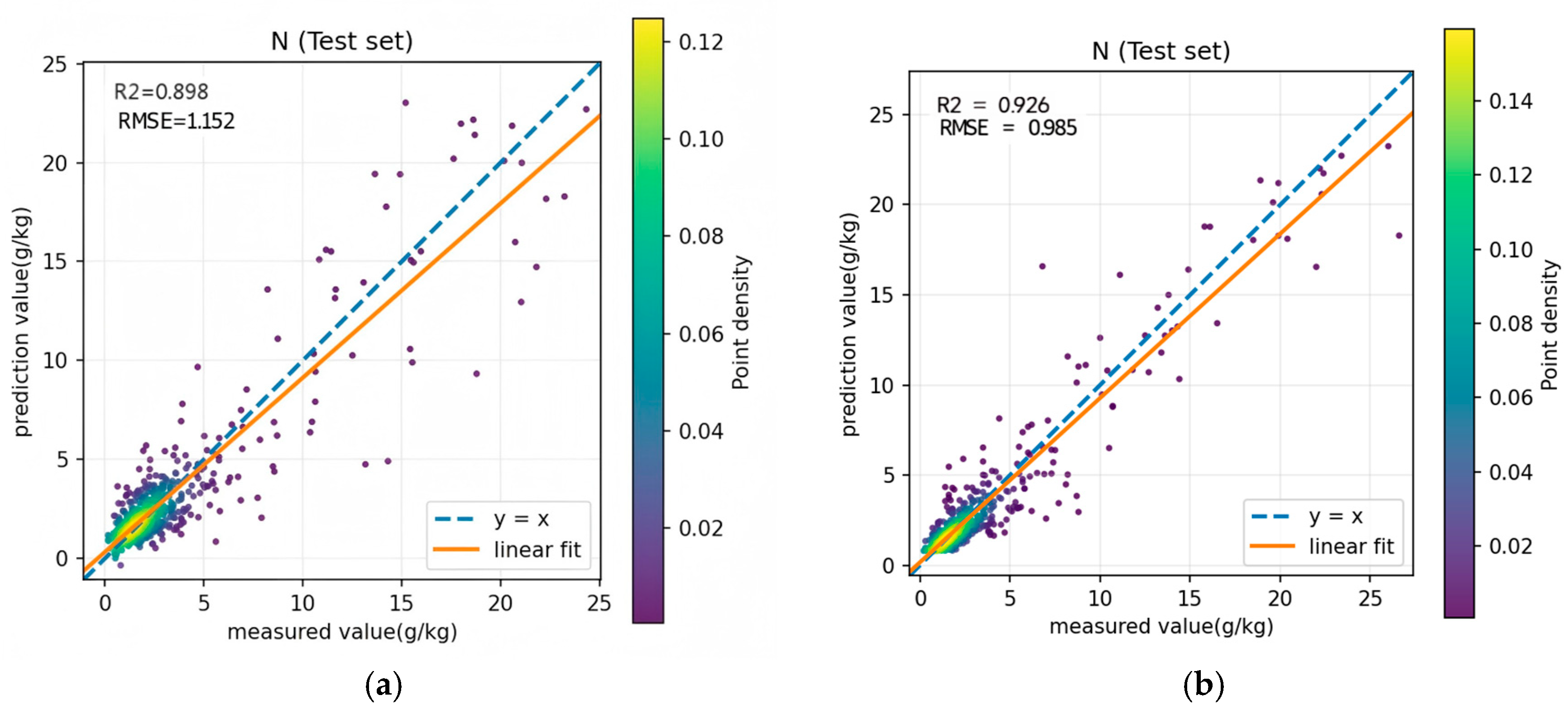
To further evaluate the prediction consistency of DGPRT-ResNet in small-sample hyperspectral soil total nitrogen prediction, the relationship between the measured and predicted values on the test set was visualized using scatter plots. The results are shown in Figure 6. The baseline ResNet and the proposed DGPRT-ResNet were compared to intuitively examine the fitting behavior of the two models.

Figure 6. Scatter plots of predicted versus measured soil total nitrogen values on the test set. (a) Baseline ResNet; (b) DGPRT-ResNet.

As shown in Figure 6, the predicted values of both models generally follow the variation trend of the measured soil total nitrogen values, and most scatter points are distributed near the ideal reference line $y=x$. This indicates that both models can capture the basic mapping relationship between hyperspectral features and soil total nitrogen content. However, compared with the baseline ResNet, the scatter distribution of DGPRT-ResNet is more concentrated around the ideal reference line, and its fitted line is closer to $y=x$. This suggests that the proposed model achieves better prediction consistency.

Specifically, the baseline ResNet achieved an $R^2$ of 0.898 and an RMSE of 1.152 on the test set, while DGPRT-ResNet achieved an $R^2$ of 0.926 and an RMSE of 0.985. The improvement in $R^2$ and the reduction in RMSE indicate that DGPRT-ResNet can more accurately characterize the relationship between spectral features and soil total nitrogen values. In particular, for the low- and medium-value ranges where most test samples are distributed, DGPRT-ResNet shows a more compact scatter distribution, suggesting better fitting ability and prediction consistency under the evaluated small-sample setting.

It can also be observed that prediction errors become relatively larger in the high-value range for both models. This is mainly because high-TN samples account for a smaller proportion of the dataset, making it more difficult for the model to fully learn their distribution characteristics. Nevertheless, DGPRT-ResNet still exhibits a prediction trend closer to the reference relationship than the baseline model, indicating improved error-control capability in the relatively sparse high-TN range under the evaluated test set.

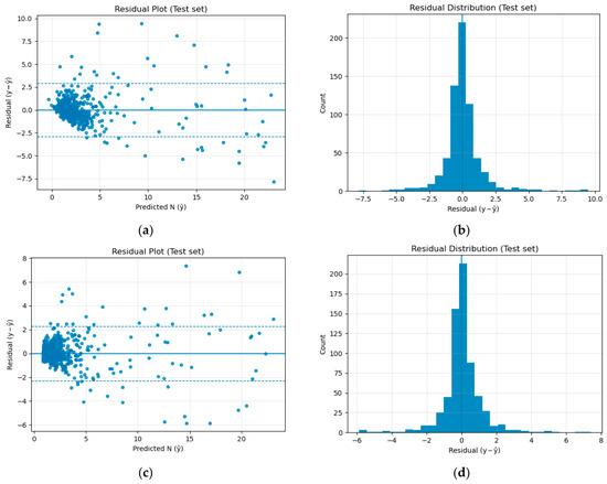
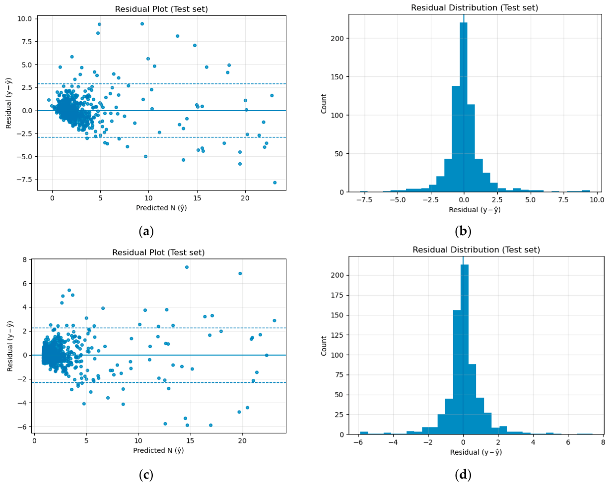
To further analyze the prediction error characteristics, residual scatter plots and residual distribution histograms were drawn, as shown in Figure 7. The residual is defined as the difference between the measured value and the predicted value. From the residual scatter plots, the residuals of both models are mainly distributed around zero, indicating that no obvious systematic deviation exists between the predicted and measured values. However, compared with the baseline ResNet, the residuals of DGPRT-ResNet are more concentrated near zero, and the degree of residual dispersion is smaller. This suggests that the proposed model can better control prediction errors and reduce residual dispersion.

Figure 7. Residual analysis of soil total nitrogen prediction on the test set. (a) Residual scatter plot of Baseline ResNet; (b) residual distribution of Baseline ResNet; (c) residual scatter plot of DGPRT-ResNet; (d) residual distribution of DGPRT-ResNet.

Combined with the variation in residuals across different prediction ranges, it can be seen that the residual fluctuation of both models tends to increase as the predicted value becomes larger. This phenomenon is related to the limited number and relatively sparse distribution of high-value samples under the small-sample setting. Compared with the baseline ResNet, DGPRT-ResNet shows smaller residual fluctuations over a wider prediction range, indicating that it has stronger modeling ability for complex spectral features and local variation information.

The residual distribution histograms further confirm this observation. The residuals of both models are mainly concentrated around zero, showing an approximately centralized distribution. However, the residual distribution of DGPRT-ResNet is sharper and more concentrated near zero, while the baseline model exhibits a relatively wider residual spread. This indicates that most prediction errors of DGPRT-ResNet are limited to a smaller range, demonstrating better error-control ability.

Overall, the scatter plots and residual analysis show that DGPRT-ResNet can improve prediction consistency and reduce residual dispersion under the evaluated test set. These results further verify that the combination of difference-guided residual calibration, prototype-regularized regression, and segmental trend reconstruction can effectively improve the representation ability of the model for soil hyperspectral data.

3.3. Comparative Experiment

To further verify the effectiveness of the proposed DGPRT-ResNet in small-sample hyperspectral soil total nitrogen prediction, several representative models were selected for comparative experiments, including SVR, VGG11, TCN, ResNet152, Transformer, DLinear, PatchTST, and iTransformer [16,17,18,19,20,21,22,23]. All models were trained and tested under the same experimental conditions, using the same preprocessing strategy, input representation, dataset partitioning, and evaluation metrics. The coefficient of determination $\left(R^2\right)$ and root mean square error (RMSE) were used to evaluate model performance. The comparative results are shown in Table 2.

Table 2. Comparative results of different models.

Model	${\mathit{R}}^2$	RMSE (g/kg)
SVR	0.873	1.246
VGG11	0.889	1.181
TCN	0.901	1.128
ResNet152	0.862	1.343
Transformer	0.907	1.096
DLinear	0.891	1.142
PatchTST	0.883	1.240
iTransformer	0.894	1.231
DGPRT-ResNet	0.926	0.985

As shown in Table 2, different models exhibit clear performance differences under the small-sample setting. The traditional machine learning model SVR achieves relatively limited performance, with an $R^2$ of 0.873 and an RMSE of 1.246. This indicates that relying only on conventional nonlinear regression is insufficient for fully capturing the complex relationship between hyperspectral features and soil total nitrogen content.

Among the deep learning models, VGG11, DLinear, PatchTST, and iTransformer obtain certain improvements over SVR, but their overall performance remains limited. This suggests that these models can extract useful spectral representations to some extent, but they may still be insufficient in modeling local spectral details, deep feature distribution structures, and global trend information under limited training samples.

TCN and Transformer show relatively better performance among the compared baseline models. TCN achieves an $R^2$ of 0.901 and an RMSE of 1.128, while Transformer obtains an $R^2$ of 0.907 and an RMSE of 1.096. These results indicate that convolution-based local sequence modeling and attention-based global dependency modeling both have advantages in hyperspectral regression tasks. However, their performance is still lower than that of DGPRT-ResNet. In addition, ResNet152 achieves an $R^2$ of 0.862 and an RMSE of 1.343, which suggests that simply increasing network depth does not necessarily improve prediction performance under small-sample conditions. On the contrary, an overly complex model may increase the risk of overfitting and reduce generalization ability.

The proposed DGPRT-ResNet achieves the best performance among all compared models, with an $R^2$ of 0.926 and an RMSE of 0.985. Compared with Transformer, DGPRT-ResNet improves $R^2$ by 0.019 and reduces RMSE by 0.111. Compared with TCN, DGPRT-ResNet improves $R^2$ by 0.025 and reduces RMSE by 0.143. These results demonstrate that DGPRT-ResNet has stronger fitting ability and error-control capability in small-sample hyperspectral soil total nitrogen prediction.

Overall, although traditional machine learning models, general convolutional networks, and sequence modeling architectures can predict soil total nitrogen to a certain extent, they still have limitations in fully exploiting local spectral variations, feature-space structures, and global trend information under small-sample conditions. In contrast, DGPRT-ResNet improves model representation from three complementary aspects: difference-guided residual calibration, prototype-regularized regression, and segmental trend reconstruction. Therefore, it achieves more accurate prediction results under the evaluated small-sample soil TN setting.

4. Discussion

The experimental results show that DGPRT-ResNet achieved the best performance in small-sample hyperspectral soil total nitrogen prediction, with higher $R^2$ and lower RMSE than the baseline ResNet and other comparison models. This indicates that the proposed model can better capture the nonlinear relationship between Vis–NIR hyperspectral features and soil total nitrogen content under limited training samples.

The improvement mainly comes from the complementary effects of DGRC, PRRH, and STRAB. DGRC enhances local spectral-shape variations by using adjacent-band difference responses, which helps the model focus on informative spectral fluctuations and band transition regions. PRRH introduces prototype-based constraints into the deep feature space, encouraging samples with similar TN values to form more compact feature distributions. STRAB further guides the network to preserve the overall spectral trend, reducing overfitting to local numerical noise under small-sample conditions.

The ablation results confirm that each module contributes positively to model performance. Among the single-module variants, STRAB provides relatively strong improvement, suggesting that global spectral trend information is important for soil TN prediction. When DGRC, PRRH, and STRAB are combined, the complete DGPRT-ResNet achieves the best result, demonstrating that local difference modeling, feature-space regularization, and trend-preserving supervision are mutually complementary.

The comparison with other models also shows that simply using general-purpose regression or deep learning architectures is not sufficient for small-sample soil hyperspectral prediction. Although TCN and Transformer perform relatively well, they still lack task-specific constraints for local spectral changes and feature distribution structure. ResNet152 performs worse than shallower models, indicating that increasing network depth does not necessarily improve generalization when training samples are limited.

Previous studies on soil spectral prediction have shown that both conventional nonlinear regression methods and deep learning models can achieve effective performance, but their effectiveness is strongly affected by sample size, spectral variability, preprocessing strategies, and model complexity. Deep learning methods generally provide stronger nonlinear representation ability, whereas conventional methods may remain competitive when the available training samples are limited. Therefore, the present study does not assume that deeper or more complex models are inherently superior, but focuses on whether task-specific constraints can improve feature learning under the evaluated limited-sample setting. The present results suggest that jointly modeling local spectral variations, embedding-space structure, and global spectral trends can provide complementary benefits for soil TN prediction when training data are limited.

Nevertheless, several limitations of the present study should be noted. First, the experiments were conducted on a 2000-sample soil TN subset derived from the LUCAS 2009 soil spectral database. Although LUCAS 2009 contains samples collected from multiple countries and regions and therefore provides considerable spatial and sample-source diversity, the present evaluation remains an in-dataset assessment for a single soil property. Accordingly, the current results should not be interpreted as direct evidence of cross-dataset, cross-property, or field-level generalization. Second, the weighting coefficients associated with prototype regularization and trend reconstruction were kept fixed throughout the reported experiments, and their sensitivity was not systematically investigated. Therefore, the present study does not make claims regarding hyperparameter robustness. Third, a fixed percentile-based stratified 7:3 training/test partition and a fixed random seed were adopted to provide a controlled and reproducible basis for model comparison. However, the reported point estimates do not characterize performance variability across independent training runs or cross-validation folds. Future work will therefore extend the evaluation to additional soil properties, independent spectral datasets, cross-regional and field-measured spectra, and will systematically investigate hyperparameter sensitivity and model variability through repeated runs or cross-validation.

In addition, a systematic computational-complexity comparison, including parameter count, training time, inference latency, and resource consumption, was not included in the present study. It should be noted that STRAB is used only during training and is removed during inference; nevertheless, the quantitative computational cost of the complete framework requires further evaluation.

Overall, DGPRT-ResNet improves small-sample hyperspectral soil TN prediction by integrating local difference enhancement, prototype-based feature regularization, and global trend reconstruction. The proposed framework provides a useful reference for small-sample spectral regression tasks.

5. Conclusions

This study proposed DGPRT-ResNet, a difference-guided and prototype-regularized residual network with a segmental trend reconstruction auxiliary branch, for small-sample hyperspectral soil total nitrogen prediction. The model integrates three complementary components: DGRC for enhancing local spectral-shape variations, PRRH for improving the structure of the deep feature space, and STRAB for preserving global spectral trend information.

Experimental results on a 2000-sample subset constructed from the LUCAS 2009 soil spectral dataset showed that DGPRT-ResNet achieved the best prediction performance among all compared models, with an ${\mathrm{R}}^2$ of 0.926 and an RMSE of 0.985 g/kg on the test set. Ablation experiments further confirmed that DGRC, PRRH, and STRAB all contributed positively to model performance, and their combination produced the most effective result.

Overall, under the evaluated fixed small-sample setting based on the LUCAS 2009 soil TN subset, DGPRT-ResNet achieved improved prediction performance by jointly considering local difference modeling, feature-space regularization, and global trend preservation. The present results support the effectiveness of the proposed architecture within this experimental setting. External generalization, sensitivity to the loss-weighting coefficients, and performance variability across independent training runs remain to be further investigated. Future work will focus on additional soil properties, independent spectral datasets, and cross-regional and field-measured spectra, together with systematic hyperparameter sensitivity analysis and repeated-run or cross-validation evaluation.

References

- Shin, S.K.; Lee, S.J.; Park, J.H. Prediction of Soil Properties Using Vis-NIR Spectroscopy Combined with Machine Learning: A Review. Sensors 2025, 25, 5045. [Google Scholar] [CrossRef] [Scilit] [PubMed]
- Morellos, A.; Pantazi, X.-E.; Moshou, D.; Alexandridis, T.; Whetton, R.; Tziotzios, G.; Wiebensohn, J.; Bill, R.; Mouazen, A.M. Machine learning based prediction of soil total nitrogen, organic carbon and moisture content by using VIS-NIR spectroscopy. Biosyst. Eng. 2016, 152, 104–116. [Google Scholar] [CrossRef] [Scilit]
- Zhang, T.; Li, Y.; Wang, M. Prediction of soil organic carbon and total nitrogen affected by mine using Vis–NIR spectroscopy coupled with machine learning algorithms in calcareous soils. Sci. Rep. 2024, 14, 28014. [Google Scholar] [CrossRef] [Scilit] [PubMed]
- Padarian, J.; Minasny, B.; McBratney, A.B. Using deep learning to predict soil properties from regional spectral data. Geoderma Reg. 2019, 16, e00198. [Google Scholar] [CrossRef] [Scilit]
- Wang, Z.; Chen, S.; Lu, R.; Zhang, X.; Ma, Y.; Shi, Z. Non-linear memory-based learning for predicting soil properties using a regional vis-NIR spectral library. Geoderma 2024, 441, 116752. [Google Scholar] [CrossRef] [Scilit]
- Angelopoulou, T.; Balafoutis, A.; Zalidis, G.; Bochtis, D. From Laboratory to Proximal Sensing Spectroscopy for Soil Organic Carbon Estimation—A Review. Sustainability 2020, 12, 443. [Google Scholar] [CrossRef] [Scilit]
- Tóth, G.; Jones, A.; Montanarella, L. (Eds.) LUCAS Topsoil Survey: Methodology, Data and Results. In JRC Technical Reports; Publications Office of the European Union: Luxembourg, 2013; EUR 26102. [Google Scholar] [CrossRef] [PubMed]
- He, K.; Zhang, X.; Ren, S.; Sun, J. Deep residual learning for image recognition. In Proceedings of the 2016 IEEE Conference on Computer Vision and Pattern Recognition (CVPR), Las Vegas, NV, USA, 27–30 June 2016; pp. 770–778. [Google Scholar] [CrossRef] [Scilit]
- Snell, J.; Swersky, K.; Zemel, R.S. Prototypical Networks for Few-Shot Learning. In Proceedings of the 31st International Conference on Neural Information Processing Systems (NIPS 2017), Long Beach, CA, USA, 4–9 December 2017; Curran Associates, Inc.: Red Hook, NY, USA, 2017; pp. 4080–4090. [Google Scholar]
- Zhang, R.; Chen, K.; Li, L.; Zhou, D.; Xu, Y.; Lin, Z.; Xu, L.; Song, W. Band-Mixed Edge-Aware Interaction Learning for RGB-T Camouflaged Object Detection. IEEE Trans. Multimed. 2026, 1–12. [Google Scholar] [CrossRef] [Scilit]
- Zhang, J.; Zhang, R.; Cao, Z.; Xu, L.; Chen, X.; Xu, M. It Takes Two: Multi-Frequency Perception With Complementary Fusion Network for Complex Scene Segmentation. IEEE Trans. Circuits Syst. Video Technol. 2026, 36, 5288–5300. [Google Scholar] [CrossRef] [Scilit]
- Heil, K.; Schmidhalter, U. An Evaluation of Different NIR-Spectral Pre-Treatments to Derive the Soil Parameters C and N of a Humus-Clay-Rich Soil. Sensors 2021, 21, 1423. [Google Scholar] [CrossRef] [Scilit] [PubMed]
- Peng, L.; Cheng, H.; Wang, L.-J.; Zhu, D. Comparisons of the prediction results of soil properties based on fuzzy c-means clustering and expert knowledge from laboratory visible–near-infrared reflectance spectroscopy data. Can. J. Soil Sci. 2021, 101, 33–44. [Google Scholar] [CrossRef] [Scilit]
- Hodson, T.O. Root-mean-square error (RMSE) or mean absolute error (MAE): When to use them or not. Geosci. Model Dev. 2022, 15, 5481–5487. [Google Scholar] [CrossRef] [Scilit]
- Karunasingha, D.S.K. Root mean square error or mean absolute error? Use their ratio as well. Inf. Sci. 2022, 585, 609–629. [Google Scholar] [CrossRef] [Scilit]
- Deiss, L.; Margenot, A.J.; Culman, S.W.; Demyan, M.S. Tuning support vector machines regression models improves prediction accuracy of soil properties in MIR spectroscopy. Geoderma 2020, 365, 114227. [Google Scholar] [CrossRef] [Scilit]
- Simonyan, K.; Zisserman, A. Very Deep Convolutional Networks for Large-Scale Image Recognition. In Proceedings of the International Conference on Learning Representations (ICLR 2015), San Diego, CA, USA, 7–9 May 2015. [Google Scholar]
- Lea, C.; Vidal, R.; Reiter, A.; Hager, G.D. Temporal Convolutional Networks: A Unified Approach to Action Segmentation. In Computer Vision—ECCV 2016 Workshops; Hua, G., Jégou, H., Eds.; Springer International Publishing: Cham, Switzerland, 2016; pp. 47–54. [Google Scholar]
- Sun, M.; Yang, Y.; Li, S.; Yin, D.; Zhong, G.; Cao, L. A study on hyperspectral soil total nitrogen inversion using a hybrid deep learning model CBiResNet-BiLSTM. Chem. Biol. Technol. Agric. 2024, 11, 157. [Google Scholar] [CrossRef] [Scilit]
- Vaswani, A.; Shazeer, N.; Parmar, N.; Uszkoreit, J.; Jones, L.; Gomez, A.N.; Kaiser, Ł.; Polosukhin, I. Attention Is All You Need. In Proceedings of the 31st International Conference on Neural Information Processing Systems (NIPS 2017), Long Beach, CA, USA, 4–9 December 2017; Curran Associates, Inc.: Red Hook, NY, USA, 2017; pp. 6000–6010. [Google Scholar]
- Zeng, A.; Chen, M.; Zhang, L.; Xu, Q. Are transformers effective for time series forecasting? Proc. AAAI Conf. Artif. Intell. 2023, 37, 11121–11128. [Google Scholar] [CrossRef] [Scilit]
- Nie, Y.; Nguyen, N.H.; Sinthong, P.; Kalagnanam, J. A Time Series Is Worth 64 Words: Long-Term Forecasting with Transformers. In Proceedings of the International Conference on Learning Representations (ICLR 2023), Kigali, Rwanda, 1–5 May 2023. [Google Scholar]
- Liu, Y.; Hu, T.; Zhang, H.; Wu, H.; Wang, S.; Ma, L.; Long, M. iTransformer: Inverted Transformers Are Effective for Time Series Forecasting. In Proceedings of the Twelfth International Conference on Learning Representations (ICLR 2024), Vienna, Austria, 7–11 May 2024. [Google Scholar]
Disclaimer/Publisher’s Note: The statements, opinions and data contained in all publications are solely those of the individual author(s) and contributor(s) and not of MDPI and/or the editor(s). MDPI and/or the editor(s) disclaim responsibility for any injury to people or property resulting from any ideas, methods, instructions or products referred to in the content. |
© 2026 by the authors. Licensee MDPI, Basel, Switzerland. This article is an open access article distributed under the terms and conditions of the Creative Commons Attribution (CC BY) license.