


Abstract
Excess indoor moisture can affect occupant health, damage building materials, and create conditions favorable to mold growth. Many monitoring systems rely on fixed thresholds and current sensor readings, offering little anticipation of unfavorable conditions. This study formulates indoor mold risk monitoring as a short-horizon forecasting problem for edge-based early warning. Recent relative humidity measurements are used to predict whether the subsequent 30 or 60 min interval is Safe, Elevated, or Mold-Favorable. A residual Temporal Convolutional Network (TCN) was compared to classical machine learning models and simple baselines using a public indoor time-series dataset. To prevent temporal leakage, the training, validation, and test sets were separated chronologically by explicit gaps. At the primary 60 min horizon, the TCN achieved a mean Macro F1 of 0.7886 and performed comparably to the strongest classical models. Robustness varied by disturbance type. The selected TCN was exported to ONNX and deployed on a Raspberry Pi 5, where the complete edge pipeline passed controlled tests and a 90 min live sensor run. The three classes represent environmental conditions associated with mold risk, not actual mold presence or biological growth. The system is therefore intended as a preventive warning tool rather than a mold-detection method.
1. Introduction
Indoor environmental quality has become a major topic of scientific, medical, and engineering interest because people spend a substantial portion of their time in homes, offices, educational institutions, and commercial buildings. Indoor environmental conditions directly influence thermal comfort, health, productivity, and building durability. Persistent dampness and mold growth are among the most common and costly indoor environmental problems, both economically and in terms of their effects on human health. Exposure to excessive indoor humidity and fungal contamination has been associated with respiratory symptoms, allergies, irritation, and reduced quality of life [1].
Mold growth in indoor spaces is a complex process governed by interactions among temperature, relative humidity, condensation, ventilation, building materials, and occupant activities such as showering, cooking without an extractor hood, and drying clothes indoors [2]. Problems are often noticed only after visible signs, characteristic odors, or material degradation appear. At that stage, intervention is more expensive and the underlying causes are more difficult to remediate. Consequently, the recent literature supports a shift from reactive observation of damage to preventive detection of conditions favorable to moisture accumulation and mold growth [3].
Recent advances in the Internet of Things (IoT), edge computing, and artificial intelligence have created new opportunities for intelligent indoor environmental monitoring. Edge platforms process data locally on compact devices, reducing cloud dependence, latency, and risks associated with continuous data transmission [4]. Artificial intelligence models can identify patterns in sensor time series and convert simple environmental measurements into actionable monitoring information. The current literature indicates that integrating low-cost sensors with edge intelligence is a promising approach to autonomous and scalable indoor monitoring [5].
In practice, many existing solutions address the problem of dampness and mold risk only partially. Such systems are frequently limited to dashboards or instantaneous threshold alerts and do not explicitly characterize how humidity evolves within a recent observation interval. Other approaches focus on general indoor air quality (IAQ) indicators and address persistent dampness only indirectly, without specifically representing operational conditions associated with mold risk [6,7]. To address this gap, the proposed system forecasts humidity conditions over a separate future interval and uses the predictions to generate local warnings on an edge device. The experimental design prevents temporal leakage and evaluates performance at both window and episode levels, including robustness to simulated sensor errors.
Detailed hygrothermal models can describe the underlying physical processes more accurately, but they often require numerous input parameters and substantial computational resources [8]. Machine learning approaches provide another option, yet many are evaluated only offline, without demonstrating integration and deployment on edge devices under real operating conditions [9]. A practical need therefore remains for reliable systems that can identify mold-favorable conditions early and operate directly in real-world settings.
In this context, the proposed system follows a hybrid edge-based design with two complementary components. The first component is a residual Temporal Convolutional Network (TCN) that uses six consecutive relative humidity observations sampled at 10 min intervals to forecast the Safe, Elevated, or Mold-Favorable state of the immediately following 30 or 60 min interval. The second component is a rule-based decision module that uses current relative humidity, dew-point depression, persistence, and hysteresis to indicate conditions approaching air saturation.
Together, the two components combine short-horizon forecasting with a physically interpretable rule for immediate critical conditions. In this study, early warning refers to anticipating future environmental conditions associated with mold risk. The system does not detect or predict biological mold growth.
The choice of a TCN over recurrent architectures, such as recurrent neural networks (RNNs), long short-term memory (LSTM) networks, and gated recurrent units (GRUs), is motivated by several technical advantages. TCNs model sequential dependencies through dilated convolutions, support efficient parallelization, and are well-suited to resource-constrained edge devices. Comparative studies have shown that TCNs can compete with or outperform recurrent architectures in various sequence-modeling tasks while offering implementation and latency advantages [10].
TCNs are established sequence models rather than a new architecture [10,11]. Their computational efficiency makes them suitable for time-series processing on edge devices. In this study, their performance is evaluated by comparing the TCN with several classical machine learning models.
To ensure that the model predicts future conditions, the input sequence and forecast target are separated in time. Six consecutive bathroom RH measurements sampled at 10 min intervals are used to predict an operational state defined from the following 30 or 60 min interval. The input and target sequences therefore do not overlap.
This study uses the Appliances Energy Prediction dataset from the UCI Machine Learning Repository [12,13]. Bathroom temperature (T5) and relative humidity (RH_5) are sampled every 10 min. The prediction target consists of three humidity-based environmental states: Safe, Elevated, and Mold-Favorable. These states are defined using RH measurements from the future 30 or 60 min interval. They represent environmental conditions associated with mold risk rather than the actual presence or growth of mold.
The main contribution of this study is an edge-based system for short-term forecasting of indoor humidity conditions. The model is compared to several classical machine learning methods using both individual prediction windows and complete humidity episodes. The experimental protocol controls temporal leakage and evaluates model robustness under simulated sensor disturbances. The forecasting model operates separately from the rule-based psychrometric module, which is used to detect immediate critical conditions.
The main contributions of this work are
- A short-term forecasting approach that uses recent RH measurements to predict Safe, Elevated, and Mold-Favorable conditions over future intervals of 30 and 60 min. The training, validation, and test sets are separated chronologically, with temporal gaps between them to prevent data leakage.
- A comparison between the residual TCN and several classical machine learning models using the same chronological data splits. The comparison considers both raw RH measurements and temporal features derived from the RH signal.
- An evaluation of the models at both window and episode levels. Additional tests examine the effects of simulated sensor noise, constant bias, missing measurements, and anomalous spikes.
- A hybrid edge-based architecture in which short-term forecasting and the detection of immediate critical conditions are handled separately. Immediate conditions are identified using a rule-based module based on RH and dew-point depression.
Together, these contributions show how a low-cost sensor and compact temporal models can extend conventional descriptive monitoring with practical, edge-based early warning for indoor environmental management.
2. Related Work
2.1. Hygrothermal and Bio-Hygrothermal Models for Mold Risk Assessment
The issue of mold growth in buildings has attracted increasing attention in scientific literature, as it lies at the intersection of several fields, such as indoor environmental monitoring, public health, building physics, and microbiology. Traditionally, mold risk assessment has relied on hygrothermal or bio-hygrothermal models, which attempt to estimate the progression of fungal growth based on factors such as temperature, relative humidity, duration of exposure, and material characteristics. These approaches have contributed significantly to understanding the mechanisms by which spores are activated and developed on building surfaces.
The VTT numerical models, developed at the VTT Technical Research Center of Finland, alongside the bio-hygrothermal models used to analyze spore behavior under variable conditions, represent a significant step forward compared to steady-state approaches. They enable the calculation of a mold index, typically based on a numerical scale corresponding to the level of fungal growth, derived from the time-dependent evolution of temperature and humidity. Studies on these models demonstrate that mold growth cannot be explained solely by a specific relative humidity value, but rather by a dynamic process dependent on the duration of exposure and the history of favorable conditions [14].
However, most of these models were initially developed under controlled laboratory conditions and calibrated for specific materials, particularly wood, using measurements taken directly at the surface level. For this reason, applying them directly in real-world homes can be challenging. In practice, sensors used in residential systems typically measure ambient air temperature and humidity without precisely capturing the conditions on the surfaces where mold actually develops. In addition, real-world environments are far more variable, influenced by factors such as ventilation, heating, thermal bridges, material types, room geometry, and even occupant behavior. Thus, the same relative humidity value measured in the air can lead to different outcomes from one space to another, depending on the local physical context.
In this context, several studies have sought to evaluate how well VTT models adapt to conditions found in real-world homes. Menneer et al. used objective measurements of air temperature and relative humidity, collected every 3–5 min over the course of a year in 219 homes, to analyze the relationship between the estimated mold index and occupant reports regarding the presence of visible mold or a characteristic odor. The results indicated that the VTT model is applicable to real-world environmental data, though its performance improves when parameters are adjusted for higher sensitivity, such as by lowering the critical humidity threshold [2].
This observation is also relevant to the present study. Although physically based models are well-founded, applying them directly to indoor environments is not always straightforward. Residential sensors typically measure ambient air temperature and humidity, whereas mold often develops in localized areas, such as cold corners or poorly ventilated surfaces, where conditions may differ from those in the rest of the room. A more flexible approach is therefore needed to accommodate real-world variation without disregarding the relevant physical processes. The method proposed here is not intended to replace detailed hygrothermal models; instead, it provides a simpler alternative that is easier to deploy and focuses on the early identification of mold-favorable conditions.
2.2. The Importance of Relative Humidity, Condensation, and Temporal Persistence
In most studies regarding mold growth, humidity is considered one of the most critical factors. Although temperature influences biological processes, relative humidity levels and conditions approaching the dew point often have a decisive impact on creating an environment favorable to fungal growth. Various studies on indoor mold prevention indicate that relative humidity can influence spore survival and activation even more than temperature, particularly when the environment undergoes repeated wetting and drying cycles [15].
This conclusion supports the idea that relative humidity should be treated as a key variable in mold risk assessment. However, a single point-in-time measurement does not always provide sufficient information. A high humidity level of short duration may represent merely a temporary phenomenon with no significant consequences, whereas the same value sustained over a prolonged period could signal the development of conditions favorable to mold growth. For this reason, modern approaches aim to account for the temporal dimension, including the duration of exposure, the influence of prior conditions, and the fact that the effects of a high-humidity episode may persist even after a temporary return to more favorable conditions.
This concept appears explicitly in memory-based models. Weisner and Collier propose an adaptation of the VTT model by introducing dynamic critical humidity thresholds influenced by prior conditions. In this approach, recent periods of high humidity can facilitate subsequent fungal growth, even under less severe conditions. In other words, mold development depends not only on the instantaneous state of the environment but also on the history of conditions to which the system has been exposed [7].
The model uses a sequence of six consecutive RH measurements to predict the environmental state over the following 30 or 60 min interval. The input sequence and future target interval do not overlap.
From this perspective, the proposed approach better reflects how the phenomenon manifests in practice compared to a system relying solely on instantaneous thresholds. Furthermore, the use of the dew point and dew-point depression establishes a direct link to the risk of condensation. Nepomuceno et al. demonstrate that the dew point can be estimated using temperature and relative humidity data and serves as a relevant indicator for condensation occurrence in residential spaces. Their study also proposes the use of sensor networks to monitor indoor moisture conditions [6]. This concept supports the approach taken in the present work, where the analysis goes beyond relative humidity values to assess how close the environment is to conditions favorable to condensation.
Dew point and dew-point depression are used in the independent rule-based safety module, while the TCN forecasting model uses only RH measurements as input. The two components serve different purposes: the TCN predicts future humidity conditions, while the rule-based module identifies critical conditions at the current time.
2.3. IoT Systems for Moisture and Mold Detection
Another important research direction in the recent literature is the use of IoT sensors to monitor the risk of dampness and mold in residential buildings. These systems emerged from the need to shift from reactive approaches, based on inspections or occupant reports following the onset of issues, toward methods capable of identifying high-risk homes or rooms at an early stage.
Bibby and Blair reported the deployment of an IoT-based monitoring system for moisture and mold detection in residential buildings across several London boroughs. Unlike laboratory-based studies, their work was validated under real operating conditions, demonstrating the practical feasibility of continuous indoor environmental monitoring. Temperature and relative humidity sensors were used to identify conditions favorable to mold growth, investigate the underlying causes of moisture problems, evaluate the effectiveness of remediation measures, and support proactive housing management. The results showed that this approach enables housing authorities to identify high-risk properties earlier, prioritize maintenance activities more effectively, and reduce reliance on repeated inspections or delayed interventions after visible damage has occurred [1].
The subsequent report, covering the 2024–2025 winter season, also offers practical insight into how these systems perform in real-world use. The findings indicate that local authorities observed clear operational benefits, alongside challenges related to interpreting risk data, integrating the systems into internal workflows, and scaling up their deployment. Instances are noted where the number of risk alerts decreased following the installation of sensors and the establishment of dedicated response teams. Furthermore, the majority of participating boroughs expressed their intention to expand the use of these systems in the future [3].
These results highlight the practical utility of IoT systems for monitoring conditions favorable to mold growth. At the same time, they also reveal an important challenge: while sensors can collect vast amounts of data, accurately interpreting the associated risk is not always straightforward. Many existing systems rely on dashboards, alerts, or rule-based decision logic, without incorporating the temporal analysis required to distinguish between brief fluctuations and persistent conditions that may indicate a genuine risk. Thus, although the practical value of sensors is clear, transforming raw data into a robust early-warning mechanism requires an intelligent component capable of interpreting how conditions evolve over time.
This study uses the same simple temperature and relative humidity sensing commonly found in IoT monitoring systems. In addition to threshold-based monitoring, the proposed system uses short-term forecasting to estimate future humidity conditions and a rule-based module to identify immediate critical conditions on the edge device.
2.4. Machine Learning for Moisture and Mold Risk Assessment in Indoor Environments
Machine learning is increasingly used in studies concerning moisture, building durability, and indoor environmental conditions, as it enables the identification of patterns that are difficult to capture using conventional methods. A significant area of focus is estimating moisture risk at the household level by utilizing data on building characteristics, energy consumption, and inspection results. Aziz and Hardy propose a predictive model for assessing moisture risk in English homes, based on 2073 records derived from inspections and energy certificates. Their study compares several machine learning algorithms, with results interpreted using the SHAP (SHapley Additive exPlanations) method to explain each variable’s contribution to the model’s output. The findings highlight factors such as heating costs, energy consumption, and wall efficiency as key elements in estimating moisture risk [16].
This study is significant because it demonstrates the potential of machine learning for identifying homes at risk of dampness. However, it relies on housing and inspection data rather than continuous indoor sensor measurements. In contrast, the approach considered here uses continuous sensor data to forecast short-term changes in indoor humidity conditions.
Another research direction found in the recent literature is the use of machine learning to approximate hygrothermal simulations and evaluate building behavior under moisture conditions. Salonvaara et al. used machine learning models to estimate the mold index and peak moisture levels within various layers of residential walls. The results showed that the proposed models could reproduce hygrothermal simulation outcomes with high accuracy, with reported R2 values exceeding 0.90, indicating excellent agreement between estimated and actual values [17].
This research direction indicates that machine learning can be useful for analyzing moisture- and mold-related problems. However, existing applications are primarily focused on simulation, design, and the performance evaluation of building components. In other words, the emphasis is placed more on analyzing building behavior than on continuous real-time monitoring using edge devices. Similarly, other studies employing neural networks to approximate hygrothermal simulations demonstrate that convolutional or recurrent models can learn complex temporal patterns of temperature, humidity, and material moisture content, thereby reducing the computational cost associated with traditional numerical simulations [9,18].
These studies show that temporal neural models can be used in moisture and hygrothermal applications, although they mainly focus on replacing or accelerating numerical simulations. In this study, temporal modeling is instead used to predict future humidity conditions from recent sensor measurements.
2.5. Deep Learning and Temporal Architectures for Indoor Environmental Monitoring
In recent years, deep learning models have been increasingly used to analyze and predict indoor environmental conditions, including air quality and indicators such as PM10 and PM2.5 particulate matter, carbon dioxide (CO2) concentration, and total volatile organic compounds (TVOC). Bakht et al. propose a hybrid model combining convolutional neural networks (CNNs), Long Short-Term Memory (LSTM) recurrent networks, and dense neural network (DNN) layers to predict PM10 and PM2.5 concentrations in subway stations. The authors argue that while classical deterministic models may require complex calculations and specialized expertise, deep learning models can learn directly from historical data and more easily capture the temporal dynamics of environmental parameters [19].
Kim et al. propose an edge computing-based monitoring system for indoor environments that utilizes 14 different types of sensors to collect environmental data. To estimate indoor air quality (IAQ) indicators, the authors employ bidirectional LSTM models, a type of recurrent neural network capable of analyzing temporal dependencies within the data. The system is implemented on the NVIDIA Jetson Nano platform and is capable of simultaneously collecting environmental data and estimating parameters such as PM2.5, TVOC, and CO2 [5].
These studies demonstrate the growing practicality of combining artificial intelligence, indoor environmental monitoring, and edge computing. However, most focus on general indoor air quality rather than persistent moisture and mold risk. They also often use recurrent architectures, such as LSTM or GRU networks, and systems with numerous sensors. In contrast, the present work uses only temperature and humidity measurements, a compact TCN, and explicitly calculated psychrometric indicators to target mold-favorable conditions.
The TCN is used because the model takes a sequence of sensor measurements as input and predicts conditions over a future interval. Dilated causal convolutions capture temporal information from previous measurements while allowing efficient parallel computation.
2.6. Implementation and Validation of AI Models on Edge Platforms
Edge computing is essential for continuous monitoring applications because it enables local data processing, reducing dependence on cloud services, communication latency, and unnecessary data transmission. In the context of smart homes or buildings, this capability is important not only for technical reasons but also for practical ones. Such a system must be capable of stable, autonomous, long-term operation on compact hardware with limited resources, even when network connectivity is poor or temporarily unavailable.
Studies on the deployment of machine learning models on embedded platforms have shown that tools such as ONNX Runtime can significantly accelerate the inference process and facilitate model execution on devices such as the Raspberry Pi with minimal performance loss. Vicente et al. compared several machine learning tools on a desktop system running Python 3.8.10 and on a Raspberry Pi running Python 3.9.2, showing that ONNX Runtime 1.14.1, used on both platforms, achieved lower inference times than conventional Python implementations and represented a suitable solution for embedded applications [4].
Computation offloading can be used when computational demands exceed local resources, but it also introduces challenges related to scheduling, task priority, and network connectivity. Priority-aware approaches have been proposed to address these issues in networked applications [20]. In the proposed system, forecasting is designed to run locally on the edge device, while remote communication is used only for optional synchronization or notifications.
Reliable edge operation also depends on how invalid, missing, or temporally inconsistent sensor data are handled. The edge implementation includes sensor retry, timestamp validation, stale-data detection, buffer reset after data gaps, local logging, and prioritized operational states.
2.7. Research Gap and Positioning of the Proposed Study
Existing approaches to moisture and mold risk assessment are diverse, but no simple, unified solution has emerged. Physical and bio-hygrothermal models, including VTT-based methods, describe mold-promoting mechanisms in detail. However, because they depend on material properties, surface conditions, and sensitivity parameters, applying them to low-cost continuous monitoring requires additional measurements and adaptation to real-world sensor data [2,21,22,23].
IoT systems for moisture and mold monitoring have demonstrated practical value, particularly in social housing and preventive building management. However, many solutions remain limited to alerts, dashboard visualization, or retrospective analysis, without adequately representing repeated humidity exceedances, temporal changes in indoor conditions, or proximity to condensation [1,3,24,25,26].
Window-based learning from ambient-sensor streams has also been demonstrated in intelligent residential environments for activity recognition, illustrating the broader applicability of temporal aggregation to continuous indoor sensor data [27].
Machine learning models have been widely applied to moisture risk estimation and hygrothermal analysis. Most of these models are designed either for building-scale assessment or for approximating hygrothermal simulations rather than for periodic real-time inference on edge devices. Deep learning methods have also been applied to indoor air quality monitoring, where temporal modeling is commonly used to analyze sensor data. However, these approaches mainly focus on pollutant prediction and general indoor environmental assessment instead of conditions associated with persistent moisture and mold growth [16,19,28,29].
The literature indicates a need for compact systems that provide short-horizon forecasting of indoor humidity conditions while supporting local edge processing [30,31]. This study addresses this need through a leakage-controlled comparison of temporal and classical machine learning models, complemented by robustness testing under simulated sensor corruption.
3. Materials and Methods
3.1. General Architecture of the Proposed System
Moisture-related conditions cannot always be characterized adequately by instantaneous measurements alone. Their evolution over time is relevant to short-term warning, while proximity to saturation provides complementary information about immediate critical conditions. The proposed system therefore combines RH-based temporal forecasting with a separate psychrometric assessment based on temperature, relative humidity, dew point, and dew-point depression.
The overall architecture of the proposed system is shown in Figure 1. Temperature and relative humidity are measured using a DHT22 sensor. The measurements are validated and organized into a consistent time series before being used by two separate components: the forecasting path and the current-condition safety path.
Figure 1.
Proposed hybrid edge architecture for indoor environmental monitoring.
The forecasting path uses the six most recent valid RH measurements, sampled at 10 min intervals. These measurements are provided to the TCN to predict the humidity state of the following 30 or 60 min interval. The forecast interval starts after the last input measurement, so the input and target sequences do not overlap. The predicted state is classified as Safe, Elevated, or Mold-Favorable.
The system also includes a separate psychrometric safety path for evaluating current conditions. It uses the current temperature and RH measurements to calculate the dew point and dew-point depression. Persistence and hysteresis are applied to determine whether the current state is Non-Critical or Critical. Critical is not included as a TCN class because it describes an immediate condition rather than a future state.
The two paths provide complementary information for the final system state. When the current condition is Non-Critical, the TCN forecast is retained. If a Critical condition is detected, it takes priority over the forecast. The final state is used for local warnings and logging.
Sensor acquisition, data validation, TCN inference, psychrometric calculations, and final-state determination are performed locally on a Raspberry Pi 5. The TCN runs through ONNX Runtime, while the safety path uses rule-based calculations on the same device. Cloud processing is therefore not required for normal operation.
3.2. Dataset Description and Leakage-Controlled Temporal Preprocessing
The experiments were conducted using the publicly available Appliances Energy Prediction dataset from the UCI Machine Learning Repository [12,13]. The dataset contains 19,735 complete observations collected in a low-energy house and averaged at 10 min intervals over approximately 4.5 months.
Among the available room-level measurements, the bathroom temperature, T5 (°C), and relative humidity, RH_5 (%), were selected because bathroom environments are particularly relevant for monitoring short-term variations in indoor humidity. The TCN forecasting model uses only RH_5 as input. The full-feature variants of the classical models additionally use T5, dew point, dew-point depression, and the first differences in all four quantities.
The source observations are already organized at regular 10 min intervals, and no missing values occur in the selected T5 and RH_5 series. Consequently, no temporal resampling or interpolation was required. The timestamps were converted into a standardized format, and the observations were arranged chronologically before the temporal data blocks and forecast pairs were constructed.
To prevent temporal leakage, the raw observations were divided chronologically into training, validation, and test blocks before scaling, feature construction, and forecast pair generation. The blocks were separated by two seven-day exclusion gaps, each containing 1008 observations. This resulted in a separation of 7 days and 10 min between the last retained observation of one block and the first retained observation of the next. Each gap is longer than the maximum input–target interval and prevents observations from being shared between adjacent subsets. After removing the two gaps, 17,719 observations remained for the three data blocks. Forecast pairs were then generated separately within each block, with no input or target interval crossing a block boundary. All generated forecast pairs maintained the required 10 min sampling continuity. Standardization parameters were fitted exclusively on the training block and then applied unchanged to the validation and test blocks.
Each input consists of six consecutive RH_5 measurements sampled at 10 min intervals. The target is defined using measurements from the following 30 or 60 min interval. The input and target sequences therefore do not overlap. Table 1 shows the chronological data blocks, the number of valid forecast pairs, and the target-class distributions for both forecast horizons.
Table 1.
Chronological data blocks, valid forecast pairs, and target-class distributions.
The proposed system uses only temperature and relative humidity as sensor measurements. RH_5 is used as input to the forecasting model, while T5 and RH_5 are used to calculate dew point and dew-point depression for the separate safety path.
3.3. Input–Target Construction and State Definitions
Each input sequence contains six consecutive RH measurements sampled at 10 min intervals. The target is defined from the subsequent 30 or 60 min interval, beginning with the first measurement after the input sequence. The input and target intervals do not overlap. Figure 2 illustrates this construction for the 60 min forecasting horizon.
Figure 2.
Input and future target intervals for the 60 min forecasting horizon.
The target class is determined exclusively from the RH measurements in the future interval, with no contribution from the input measurements. The labeling criteria used to define the three operational states are summarized in Table 2.
Table 2.
Definition of operational states for future target labeling.
With three target measurements at the 30 min horizon, these criteria correspond to at least one measurement with RH ≥ 66% for Mold-Favorable and at least two measurements with RH ≥ 61% for Elevated, provided that the Mold-Favorable criterion is not satisfied; with six target measurements at the 60 min horizon, the corresponding minimum counts are two and three measurements, respectively.
The selected RH thresholds were defined as operational early-warning limits rather than as biological thresholds for mold growth. Indoor moisture-control guidance recommends maintaining relative humidity below 60% [32], while critical humidity conditions for mold growth depend on factors such as temperature, exposure duration, and material sensitivity [14,21,22,23]. Accordingly, 61% RH was selected to indicate a departure from the recommended indoor humidity range, while 66% RH defines a higher warning level. These thresholds are therefore used as engineering criteria for graded environmental monitoring and should not be interpreted as direct biological limits for mold growth.
3.4. Psychrometric and Dynamic Feature Engineering
For the full-feature classical models, the raw temperature and relative humidity measurements were complemented by several derived features that provide additional information about the indoor environment. These features describe psychrometric conditions and changes between consecutive measurements without requiring additional sensors. In total, each time sample is represented by eight features: temperature, relative humidity, dew point, dew-point depression, and the temporal changes in these four variables between consecutive measurements.
The dew point was calculated from temperature and relative humidity using the Magnus formula, which provides a practical balance between simplicity and accuracy in environmental monitoring. The intermediate parameter γ is defined by Equation (1), and the dew-point temperature by Equation (2):
where T represents the ambient temperature (°C), RH is the relative humidity (%), and the constants are a = 17.62 and b = 243.12.
The dew point is the temperature at which the air becomes saturated and condensation begins to occur. It therefore indicates how close the indoor environment is to conditions that favor moisture accumulation.
The difference between the ambient temperature and the dew point was then calculated using Equation (3).
Dew-point depression is the difference between the ambient temperature and the dew point. Smaller values of Δ indicate greater proximity to saturation and condensation, whereas larger values indicate a greater distance from these conditions.
Changes between consecutive measurements were also calculated for temperature, relative humidity, dew point, and dew-point depression. These differences describe how each variable changes from one measurement to the next. They were calculated separately within each chronological data block, so no future measurements or data from another block were used.
The resulting full-feature set contains eight variables: temperature, relative humidity, dew point, dew-point depression, and the first differences in these four quantities. These features are used for classical model comparisons, while the TCN uses only the RH_5 sequence described in Section 3.3. Dew point and dew-point depression are also used in the separate rule-based safety module to evaluate current conditions.
3.5. Development and Implementation of the TCN Model
A Temporal Convolutional Network (TCN) was used to forecast the future operational state. TCNs are well-suited to this task because they can model temporal dependencies using one-dimensional convolutions while maintaining relatively low computational complexity and efficient inference, making them appropriate for edge-oriented applications.
The architecture is illustrated in Figure 3. The TCN uses a six-sample RH_5 sequence as input. In the residual blocks, k denotes the kernel size and d the dilation factor. Increasing the dilation factor allows the network to use a wider temporal context without increasing the kernel size. The initial convolution is followed by batch normalization and ReLU activation, while each residual block contains two convolutional layers with batch normalization, ReLU activation, and a dropout rate of 0.10. The classification head includes ReLU activation and a dropout rate of 0.20 before producing the three-class output.
Figure 3.
Architecture of the RH-only residual TCN for future-state forecasting.
The TCN was trained independently with five random seeds using the settings listed in Table 3. For each run, the checkpoint with the highest validation Macro F1 was selected, with validation loss used only in case of a tie. The test block was evaluated only after model selection and was not used for training or checkpoint selection. The same architecture and training settings were used for both the 30 and 60 min forecast horizons.
Table 3.
TCN training and model-selection configuration.
Figure 4 illustrates the training and validation behavior for the 60 min TCN run with seed 33. This run had the median validation Macro F1 among the five seeds and is shown as a representative example. The selected checkpoint occurred at epoch 18, based on validation Macro F1.
Figure 4.
Training and validation curves for the representative 60 min TCN run. The dashed vertical line in both panels marks the selected checkpoint at epoch 18.
3.6. Classical Baselines and Handcrafted Temporal Features
All baselines use the same chronological blocks, exclusion gaps, forecast pairs, and target definitions as the TCN. The Majority Safe baseline always predicts Safe and serves as a simple reference for the imbalanced dataset. The Persistence baseline uses the operational state of the most recent interval as the prediction for the future interval. For the 30 min forecast, this state is calculated from the three most recent RH measurements, while the 60 min forecast uses all six measurements from the input sequence. All learned models received the complete six-observation input sequence at both forecasting horizons. The classical models include Logistic Regression (LR), Random Forest (RF), XGBoost (XGB), and Histogram-Based Gradient Boosting (HGB).
The LR, RF, and XGB hyperparameters were selected from predefined grids using validation Macro F1, without access to the test results. RF and XGB were evaluated using the same five random seeds as the TCN, while LR and HGB were evaluated once per configuration. Each model was trained and evaluated independently for the 30 and 60 min forecasting horizons.
Two raw-input configurations were considered. The RH-only configuration contains the six ordered RH_5 measurements from the input sequence.
The full configuration contains six temporal positions for each of the eight features described in Section 3.4, resulting in a 6 × 8 input that was flattened into a 48-dimensional vector for the classical models. Flattening preserves the temporal position of each value but does not impose the convolutional weight sharing used by the TCN.
To examine whether explicit temporal summaries improved the classical models, additional engineered representations were constructed exclusively from the historical input sequence. No observations from the future target interval were used to calculate these features.
For the engineered RH configuration, seven temporal features were calculated from the six RH_5 measurements: mean, variance, minimum, maximum, range, linear slope, and net change. The slope was calculated across the six time steps, and net change was defined as the difference between the last and first measurements. Four additional features were calculated for the 61% and 66% RH thresholds: the total time at or above each threshold and the longest consecutive period at or above it. Each qualifying measurement represents 10 min. Together with the six original RH_5 measurements, these features give a total of 17 variables.
For the full handcrafted configuration, the seven temporal summaries were calculated separately for each of the eight input features. Together with the 48 raw lagged values and the four RH duration/run variables, this produced a total of 108 variables. Raw lagged values were standardized channel-wise using parameters fitted exclusively on the training data. Within the engineered representations, each added summary variable was standardized using its own parameters fitted to the training windows. All fitted transformations were then applied unchanged to the validation and test sets.
For each classical model, the raw and handcrafted representations were compared using validation Macro F1, while the test block remained isolated from feature and hyperparameter selection. Unlike LR, RF, and XGB, whose raw benchmark configurations had already been selected through validation-based grid searches, HGB used a fixed configuration in the main benchmark. Therefore, for the paired raw-versus-handcrafted comparison, the HGB hyperparameters were selected independently for each representation using only the validation block and the same search procedure. These secondary HGB estimates were reported separately from the fixed-configuration results in the main benchmark. Table 4 summarizes the four classical input configurations.
Table 4.
Classical baseline input configurations.
3.7. Evaluation Metrics and Episode Analysis
Window-level performance was evaluated using accuracy, balanced accuracy, and Macro F1. Macro F1 was used as the primary comparison metric because Safe targets dominate the class distribution and overall accuracy can therefore obscure poor performance on the two warning classes. For models evaluated across five training seeds, window-level metrics were averaged across the five runs, and the standard deviation of Macro F1 was also reported.
Changed-state Macro F1 was also calculated for forecast pairs in which the future target class differed from the current state. The current state was determined using the same labeling rules as the future target and an interval of the same duration. For the 30 min horizon, it was calculated from the three most recent RH measurements, while the 60 min horizon used all six measurements from the input sequence. The learned models received the complete six-measurement input sequence at both horizons.
Episode-level analysis was used to assess early-warning behavior. A risk-onset episode was defined as a contiguous sequence of forecast pairs in which the current state was Safe and the future state was Elevated or Mold-Favorable. A forecast was considered positive when the predicted class was Elevated or Mold-Favorable. An onset episode was considered detected if at least one positive forecast occurred during that sequence.
A false-alert episode was defined as a contiguous sequence of positive forecasts for which the current state was Safe but the future target remained Safe. At the episode level, a detected onset episode was counted as a true positive, a missed onset episode as a false negative, and a false-alert episode as a false positive. Episode precision, recall, and F1 score were calculated from these counts. The number of false-alert episodes was also reported as an indication of the operational alert burden.
For each detected onset episode, lead time was measured from the earliest positive forecast to the first subsequent time at which the current state became Elevated or Mold-Favorable. The same horizon-specific state definition was used to determine this arrival state. Because the data are sampled at 10 min intervals, lead time is measured at this temporal resolution and does not necessarily equal the nominal 30 or 60 min forecasting horizon.
3.8. Robustness Evaluation
The robustness results reported in this study focus on the primary 60 min forecast horizon. The secondary 30 min horizon was retained for the clean-test model comparison and was not used to draw deployment-oriented robustness conclusions. For the 60 min horizon, the frozen model instances were evaluated without retraining under 13 RH input conditions. These included clean measurements, zero-mean Gaussian noise with standard deviations of 0.5, 1, and 2 percentage points (pp), and constant biases of −1, −2, +1, and +2 pp. Random dropout was tested at rates of 10% and 20%, with missing values replaced using last-observation-carried-forward (LOCF) imputation. The most recent one or two measurements were also removed and replaced using LOCF. Finally, the models were tested with 1% randomly positioned spikes of ±10 pp.
Gaussian noise, random dropout, and spike conditions were tested using 10 independent perturbation realizations. For each perturbation realization, all frozen model instances received the same modified RH sequences. Metrics were calculated separately for each model instance and realization and then averaged for each model family. Models trained with five different seeds therefore produced 50 evaluations per stochastic condition (five seeds × 10 perturbation realizations), while models trained once produced 10 evaluations. The constant-bias and missing-recent-measurement conditions are deterministic and were therefore tested once for each frozen model instance. Future target labels were kept unchanged in all robustness tests.
After perturbation, RH values were limited to the valid range of 0–100%. Missing measurements were replaced using LOCF. When no previous measurement was available, the mean RH of the training block was used instead. For the full-feature classical models, dew point, dew-point depression, and the affected first differences were recalculated from the modified RH values. This ensured that these derived features reflected the same simulated sensor error as the RH measurements.
3.9. Psychrometric Critical-State and Fault-Handling Logic
Sensor measurements are acquired at 5 min intervals for psychrometric safety monitoring and fault handling. Every second valid acquisition is added to the forecasting buffer, providing the Temporal Convolutional Network (TCN) with a sequence of six relative humidity (RH) observations sampled at 10 min intervals. These six observations are used to forecast the state of the subsequent 60 min interval as Safe, Elevated, or Mold-Favorable.
In parallel with the forecasting path, a separate psychrometric module evaluates current conditions approaching saturation. Dew-point temperature is calculated from the measured air temperature and RH using the Magnus approximation, and dew-point depression is defined in Equation (3). Critical is determined using fixed rules and is not included as a fourth TCN class. The system enters Critical when both conditions—RH ≥ 85% and Δ ≤ 3 °C—remain continuously satisfied for 20 min, starting with the first qualifying measurement. Critical is released when either condition—RH ≤ 80% or Δ ≥ 4 °C—remains continuously satisfied for 15 min. The different entry and release thresholds provide hysteresis, while the confirmation periods prevent brief threshold crossings from changing the state. If the entry or release condition is interrupted before the required time is reached, the corresponding timer is reset. Because Critical represents an immediate current condition, it overrides the TCN forecast whenever active.
The runtime uses the following state priority: Sensor Fault, Critical, WARMUP, and TCN forecast. For each scheduled DHT22 measurement, the system makes up to three read attempts. If all three attempts fail or return invalid data, Sensor Fault is activated. Sensor Fault is also triggered by a non-monotonic timestamp, a gap between valid measurements longer than 7.5 min, or stale data for more than 7.5 min. When a fault occurs, the TCN output is suppressed, the six-sample forecasting buffer and Critical-state timers are cleared, and the reason for the fault is logged. After the first valid measurement is received, the forecasting path returns to WARMUP. Six new consecutive buffered RH observations at 10 min intervals are required before TCN forecasting resumes.
Inference, psychrometric calculations, state prioritization, terminal display, and CSV logging are performed locally on the Raspberry Pi 5 without requiring continuous Internet connectivity. The terminal was used to monitor the system during prototype testing. The corresponding operational states and local actions are summarized in Table 5.
Table 5.
Operational states and local actions in the Raspberry Pi 5 edge device (Raspberry Pi Ltd., Cambridge, UK).
4. Results
4.1. Model Comparison on the Clean Held-Out Test Set
Figure 5 shows the clean-test Macro F1 scores at both forecast horizons, while Table 6 and Table 7 report the corresponding numerical results. Performance was generally higher at 30 min than at 60 min across the evaluated model families.
Figure 5.
Clean-test Macro F1 at the 30- and 60 min forecast horizons. Error bars show one standard deviation for models trained with five different seeds and are omitted for models trained once.
Table 6.
Primary 60 min clean held-out test results.
Table 7.
Secondary 30 min clean held-out test results.
The 60 min horizon was treated as the primary forecast horizon, while the 30 min horizon was included as a secondary analysis.
At the primary 60 min horizon, the TCN achieved the highest mean Macro F1 in Table 6, with a score of 0.7886. Full-feature HGB reached 0.7852, only 0.0034 lower, while RH-only HGB reached 0.7823, a difference of 0.0063. These small margins indicate that the TCN was competitive with the strongest classical models but did not clearly outperform them.
TCN, RF, and XGB results were averaged across five training seeds, while HGB and LR were fitted once. For models evaluated with five seeds, Macro F1 is reported as the mean ± one standard deviation. Episode-level results were also averaged across the five seeds. For configurations evaluated across five seeds, the reported lead time represents the mean of the five seed-specific median lead times. For configurations evaluated once, the single-run median is reported. A dash indicates that lead time is not applicable because no risk-onset episode was detected.
At the 60 min horizon, RH-only LR achieved the highest balanced accuracy (79.27%), despite having a substantially lower Macro F1 than the strongest TCN and tree-based configurations.
At the 60 min horizon, the TCN achieved a changed-state Macro F1 of 0.5555, compared to an overall Macro F1 of 0.7886. This indicates that transitions between states were more difficult to predict than the test set as a whole. Across the five TCN runs, episode precision was 0.7996, recall was 0.9565, and Episode F1 was 0.8703, with an average of 5.6 false-alert episodes. The mean of the run-level median lead times was 12 min.
Full-feature HGB achieved the highest Episode F1 at this horizon (0.8800), with five false-alert episodes and a median lead time of 10 min. RH-only XGB reached an Episode F1 of 0.8662, with an average of 5.8 false-alert episodes and a mean run-level median lead time of 10 min. Episode-level results were therefore similar for the TCN and the strongest classical models. The 60 min forecast horizon describes the duration of the future target interval and should not be interpreted as a 60 min warning lead.
Results for the secondary 30 min horizon are presented in Table 7. All model configurations achieved higher Macro F1 scores than at the 60 min horizon, although their relative ranking changed.
At the 30 min horizon, RH-only HGB achieved the highest test Macro F1 (0.8595), followed closely by RH-only XGB (0.8587) and RH-only RF (0.8505). The TCN reached a Macro F1 of 0.8382, below the best-performing classical models at this horizon.
Using the full-feature set did not consistently improve Macro F1. At 60 min, it improved the results for HGB, XGB, and LR but reduced the performance of RF. At 30 min, only LR performed better with the full-feature set, while HGB, XGB, and RF achieved higher Macro F1 with RH-only input. Overall, the TCN achieved the highest Macro F1 at the primary 60 min horizon, but the differences from the strongest classical models were small. At 30 min, the classical ensemble models achieved the highest Macro F1 scores.
4.2. Sensor-Corruption Robustness
Because the 60 min forecast horizon was designated as the primary operational setting, the extended robustness analysis focused on this horizon. The 30 min horizon was retained as a secondary clean-test comparison in Section 4.1 and was not included in the extended corruption analysis. Figure 6 compares the RH-only TCN, HGB, and XGBoost configurations under the evaluated sensor disturbances, while Table 8 provides the complete results for all configurations and the Persistence baseline.
Figure 6.
Sensor-corruption robustness at the primary 60 min forecast horizon for the RH-only TCN, HGB, and XGBoost configurations.
Table 8.
Macro F1 under the 13 input conditions evaluated at the primary 60 min forecast horizon.
Sensor corruptions were applied only to the input histories, while the corresponding target labels remained unchanged. Under clean conditions, the TCN achieved a Macro F1 of 0.7886. Its performance decreased to 0.6984 with Gaussian noise of σ = 1 pp and to 0.5956 with σ = 2 pp. Under the same conditions, RH-only XGBoost retained Macro F1 values of 0.7330 and 0.6823, respectively, representing the strongest performance among the evaluated configurations at these two noise levels.
The loss of the most recent measurements produced substantially greater degradation than randomly distributed missing values. When the latest two readings were unavailable, all learned models showed a marked reduction in Macro F1, with RH-only HGB retaining the highest score (0.6189). In contrast, random dropout followed by LOCF caused a smaller decrease even at the 20% level. The spike condition was also comparatively mild, indicating that occasional isolated outliers were less damaging than the loss of the most recent temporal information.
The effects of constant RH bias were asymmetric, with negative bias generally causing greater degradation than the corresponding positive bias across the learned configurations. For example, the TCN reached 0.6492 at −2 pp, compared to 0.7256 at +2 pp. This asymmetry may occur because negative bias shifts threshold-adjacent RH histories toward patterns associated with lower-risk states, consequently increasing the frequency of Safe predictions.
No single model performed best under every corruption condition. The TCN achieved the highest mean Macro F1 on clean data, RH-only XGBoost performed best under Gaussian noise at σ = 1 and 2 pp, and RH-only HGB achieved the highest score when the latest two measurements were unavailable. These results show that the relative performance of the models depends on the type of sensor error. In practice, this makes sensor calibration and the detection of missing or stale measurements important for maintaining reliable predictions.
4.3. Handcrafted Temporal-Feature Baselines
To determine whether the classical models benefited from explicit temporal summaries, Table 9 compares the raw lagged representation with a handcrafted representation containing statistical, trend, and high-humidity duration features. Both representations were evaluated using the same leakage-controlled chronological split, and representation preference was assessed exclusively through validation Macro F1. Because the 60 min horizon was designated as the primary operational setting, the detailed paired comparison is reported for this horizon. In Table 9, full-feature denotes features derived from all eight input features, whereas RH-only uses information derived exclusively from relative humidity. The Test Δ column reports Test handcrafted minus Test raw, expressed in percentage points and calculated using the unrounded Macro F1 values.
Table 9.
Validation and held-out test Macro F1 for the raw and handcrafted temporal representations at the primary 60 min forecast horizon.
The raw representation achieved a higher validation Macro F1 in seven of the eight model–input combinations. The only exception was RH-only LR, for which the handcrafted representation increased validation Macro F1 from 0.6110 to 0.6402. On the held-out test block, full-feature HGB achieved the highest Macro F1 among the handcrafted configurations, with a score of 0.7688. For comparison, the TCN achieved 0.7886 in the primary benchmark.
The handcrafted representation did not improve all model families. Test Macro F1 decreased for both HGB and XGBoost, while RH-only LR improved substantially, consistent with its validation result. RF also achieved higher test Macro F1 with the handcrafted representation, although its validation scores were lower. Based on the predefined validation criterion, the handcrafted RF configurations would therefore not have been selected.
For the paired comparison in Table 9, the HGB hyperparameters were reselected separately for the raw and handcrafted representations using only the validation block and the same search procedure. Consequently, its raw-input results in Table 9 differ from those of the fixed HGB configurations used in the primary benchmark. No test information was used for hyperparameter or representation selection, and these secondary estimates do not replace the primary benchmark results. Overall, the handcrafted temporal features did not provide a consistent improvement across the evaluated models, although their benefit for RH-only LR suggests that explicit temporal summaries may help simpler linear models.
4.4. Objectively Selected Test Scenarios
Figure 7 presents three complete 24 h segments selected from the held-out test block without using model prediction errors. The first segment had the highest fraction of RH measurements at or above 66%, while the second had the lowest mean RH. For the third scenario, only days containing all three ground-truth states were considered, and the day with mean RH closest to the median of this subset was selected. The resulting high-exposure, low-mean-RH, and representative three-state scenarios are shown in Figure 7a–c.
Figure 7.
Observed RH and future-state sequences for three objectively selected 24 h scenarios from the held-out test block: (a) highest RH ≥ 66% exposure; (b) lowest daily mean RH; (c) representative three-state day.
Seed 33 was used for the TCN because its validation Macro F1 was the median of the five evaluated seeds. The HGB RH-only configuration was included as the classical comparator because it uses the same six RH measurements as the TCN and achieved the highest Macro F1 among the input-matched classical models at the primary 60 min horizon. Other models were omitted to keep the figure readable. Neither the scenarios nor the TCN seed were selected using segment-level test performance.
Each categorical band in Figure 7 refers to the subsequent 60 min target interval associated with the preceding six-observation RH input sequence. The RH curve, in contrast, shows the value available at the forecast issue time. Because the ground-truth class is determined from the following 60 min rather than from the current RH value, a state transition may appear while the RH curve is still below the 61% or 66% thresholds. Critical is not shown because it is a current-condition override rather than a forecast class.
The corresponding scenario-level metrics are reported in Table 10. Scenario-level Macro F1 was calculated using the fixed three-class label set employed in the main evaluation, while MF denotes Mold-Favorable in the onset-count columns.
Table 10.
Window-level performance and Mold-Favorable onset counts for the three scenarios shown in Figure 7.
In the high-exposure scenario, both models detected the two main Mold-Favorable episodes, with the TCN achieving slightly higher window-level scores. The low-mean-RH scenario consisted mainly of Safe conditions, with only a brief Mold-Favorable episode in the evening. Both models achieved high accuracy but lower Macro F1 in this scenario. The TCN matched the single ground-truth onset, whereas HGB RH-only split it into two short predicted onsets.
In the representative three-state scenario, the HGB RH-only configuration followed the ground-truth state sequence more closely than the TCN. Both models, however, split the single Mold-Favorable episode into two predicted onsets. These scenario plots complement the complete held-out test results by showing where the model forecasts differ over time.
4.5. Raspberry Pi 5 Edge Deployment and Runtime Validation
The selected 6 × 1 RH-only TCN was exported to ONNX opset 18 under Python 3.13.15 using PyTorch 2.11.0+cpu and validated using ONNX 1.22.0. ONNX Runtime 1.29.0 was used for parity testing and for deployment on a Raspberry Pi 5 with 4 GB RAM running Python 3.11.2 with the CPUExecutionProvider.
The deployed network contained 77,443 parameters, and the ONNX model occupied 309,944 bytes (approximately 303 KiB). PyTorch–ONNX parity was evaluated on all 3534 held-out 60 min test windows before deployment.
Runtime evaluation included four tests: model-only inference, the complete software decision path, controlled functional validation, and a 90 min live sensor run. For the timing benchmarks, 200 warm-up iterations were followed by 10,000 timed executions using single-threaded ONNX inference, with latency reported as the median and 95th percentile (p95). The complete software decision path included measurement validation, Magnus psychrometric calculations, Critical-state logic, RH scaling, ONNX inference, softmax conversion, and final-state prioritization. Sensor and file input/output were excluded from this benchmark. The deployment and runtime results are summarized in Table 11.
Table 11.
Raspberry Pi 5 deployment and runtime-validation results.
Controlled functional validation used predefined sensor sequences to test the main state transitions and recovery behavior of the deployed edge runtime and ONNX model. The tests covered WARMUP and forecast cadence, Critical entry and release, persistence reset, Critical override, Sensor Fault activation, stale and invalid data handling, excessive sample gaps, non-monotonic timestamps, and recovery after a fault. In Figure 8, downward triangles indicate the times when TCN forecasts were issued. The labels E1–E6 identify the main operational events: E1 marks the first forecast after WARMUP; E2, Critical entry after the 20 min confirmation period; E3, Critical release after the 15 min confirmation period; E4, Sensor Fault entry; E5, the first valid measurement after the fault and return to WARMUP; and E6, forecast resumption after the six-sample input buffer was rebuilt.
Figure 8.
Controlled on-device functional validation of the Raspberry Pi 5 edge runtime: (a) controlled RH input and Critical-state thresholds; (b) controlled dew-point-depression input and corresponding thresholds; (c) TCN forecast and final prioritized system state during override, fault, and recovery. The gray hatched band in panels (a,b) indicates the interval with no valid sensor measurement.
During the 90 min live run, forecasting began after the required WARMUP period, and no Sensor Fault or Critical transition occurred under the observed ambient conditions. Complete live-cycle timing was dominated by sensor acquisition, while the local software decision path required only a small fraction of the 10 min forecasting interval.
5. Discussion
The forecasting task separates the historical input from the future interval being predicted. Each prediction uses a historical input sequence, while the target is calculated exclusively from the subsequent 30 or 60 min interval. Chronological train, validation, and test blocks, explicit exclusion gaps, and training-only scaling further protect the evaluation from temporal leakage. The resulting performance therefore reflects prediction of a separate future interval rather than reconstruction of the measurements used as model input.
At the primary 60 min horizon, the RH-only TCN achieved the highest mean clean-test Macro F1 of 0.7886 ± 0.0135 and remained competitive with the strongest classical alternatives. Full-feature and RH-only HGB produced closely comparable results, indicating that increasing input complexity did not provide a consistent advantage. The feature-comparison experiments led to the same general conclusion, supporting the use of a compact RH-only representation for the deployed TCN. The higher scores obtained at the secondary 30 min horizon are also consistent with the lower uncertainty associated with forecasting a shorter future interval.
The complementary episode-level and robustness analyses provide information that is not captured by clean-test Macro F1 alone. Episode-level evaluation showed that the TCN detected most true onset episodes and provided anticipatory information before many state transitions. Under simulated sensor corruption, however, model ranking depended on the disturbance type, and no single estimator dominated under all conditions. This result is relevant for deployment because sensor calibration, missing-data handling, and the expected measurement-error regime can influence the most appropriate model choice. Time-varying sensor drift was not included in the present robustness protocol and should be evaluated in longer deployments together with periodic calibration checks.
The Critical-state path has a different role from the TCN forecast. It uses current psychrometric conditions to detect situations approaching saturation, whereas the TCN predicts the humidity state of a future interval. This separation was maintained in the Raspberry Pi implementation, where Critical takes priority over the forecast when its conditions are met. On-device tests verified the Critical-state transitions, fault handling, and recovery behavior. The timing measurements showed that the computational cost was negligible compared to the 10 min forecasting interval, and the 90 min live run completed continuous sensor acquisition, forecasting, state prioritization, and local logging without failed read attempts.
The forecasting analysis is based on measurements from one indoor location over approximately 4.5 months, so broader generalization across buildings, seasons, and operating conditions remains to be established. Moreover, the Safe, Elevated, and Mold-Favorable classes represent humidity-defined environmental conditions associated with mold risk rather than direct observations of biological mold growth. The Critical rule should likewise be interpreted as an operational psychrometric warning. The 90 min Raspberry Pi run confirmed that the prototype could operate continuously during the test period, but longer field tests are needed to evaluate its reliability over time.
The results show that short-horizon humidity forecasting and rule-based assessment of current Critical conditions can be combined on an edge device. The RH-only TCN provides competitive forecasting performance with a simple input representation, while the robustness analysis and classical baselines show that model choice may depend on the expected sensor conditions. Future work should focus on longer field deployments across additional buildings and seasons, together with independent physical or microbiological measurements to validate the operational warning states. The successful ONNX deployment and on-device validation provide a practical foundation for these longer-term evaluations.
6. Conclusions
This study developed an edge-based system for the short-term forecasting of indoor humidity states associated with mold-favorable conditions. The RH-only TCN achieved the highest mean clean-test Macro F1 at the primary 60 min horizon, with results close to those of the best classical models. The robustness analysis also showed that the relative performance of the models changed under different sensor conditions.
The selected TCN was exported to ONNX and deployed on a Raspberry Pi 5 together with a separate rule-based module for detecting current Critical conditions. Controlled validation and live operation showed that forecasting, current-condition assessment, fault handling, state prioritization, and local logging can all run locally on the edge device with low computational overhead.
Overall, the proposed system provides a practical basis for edge-based early warning of humidity-defined indoor conditions associated with mold risk.
Author Contributions
Conceptualization, P.N. and Ș.O.; methodology, P.N.; software, P.N.; validation, P.N., I.A.P. and Ș.O.; formal analysis, P.N.; investigation, P.N.; resources, P.N. and Ș.O.; data curation, P.N.; writing—original draft preparation, P.N.; writing—review and editing, I.A.P. and Ș.O.; visualization, P.N. and Ș.O.; supervision, Ș.O.; project administration, Ș.O. All authors have read and agreed to the published version of the manuscript.
Funding
This research received no external funding.
Institutional Review Board Statement
Not applicable. This study did not involve humans or animals.
Informed Consent Statement
Not applicable.
Data Availability Statement
The Appliances Energy Prediction dataset is publicly available from the UCI Machine Learning Repository at https://doi.org/10.24432/C5VC8G (accessed on 26 August 2026) under CC BY 4.0. Processed forecast pairs, predictions, and analysis outputs are available from the corresponding authors upon reasonable request.
Acknowledgments
OpenAI ChatGPT, using the GPT-5.5 and GPT-5.6 Sol models, was used to assist with English-language editing and text reformulation, and to provide coding support for selected portions of the Python workflow, including code review and debugging. All AI-assisted outputs were critically reviewed, tested, and validated by the authors. The authors take full responsibility for the final manuscript, code, analyses, and reported results.
Conflicts of Interest
The authors declare no conflicts of interest.
Abbreviations
The following abbreviations are used in this manuscript:
| AI | Artificial Intelligence |
| CNN | Convolutional Neural Network |
| CPU | Central Processing Unit |
| CSV | Comma-Separated Values |
| DHT22 | Digital temperature and humidity sensor |
| DNN | Dense Neural Network |
| GAP | Global Average Pooling |
| GRU | Gated Recurrent Unit |
| HGB | Histogram-Based Gradient Boosting |
| IAQ | Indoor air quality |
| IEQ | Indoor Environmental Quality |
| IoT | Internet of Things |
| LOCF | Last Observation Carried Forward |
| LR | Logistic Regression |
| LSTM | Long Short-Term Memory |
| ONNX | Open Neural Network Exchange |
| p95 | 95th Percentile |
| pp | percentage points |
| RAM | Random-Access Memory |
| ReLU | Rectified Linear Unit |
| RF | Random Forest |
| RH | Relative humidity |
| RNN | Recurrent Neural Network |
| RSS | Resident Set Size |
| SHAP | SHapley Additive exPlanations |
| TCN | Temporal Convolutional Network |
| TVOC | Total Volatile Organic Compounds |
| UCI | University of California, Irvine |
| VTT | VTT Technical Research Center of Finland |
| XGB | XGBoost |
| Δ | Dew-point depression |
References
- Bibby, W.; Blair, L. Internet of Things (IoT) Sensors for Damp and Mould: A Comprehensive Review of Insights and Lessons Across London Boroughs; London Office for Technology and Innovation (LOTI): London, UK, 2025; Version 1.02. [Google Scholar]
- Menneer, T.; Mueller, M.; Sharpe, R.A.; Townley, S. Modelling mould growth in domestic environments using relative humidity and temperature. Build. Environ. 2022, 208, 108583. [Google Scholar] [CrossRef] [Scilit]
- Bibby, W.; Blair, L. Internet of Things (IoT) Sensors for Damp and Mould (Follow-Up): Insights from Winter Deployment and Borough Plans for the Future; Anthill Collective; London Office for Technology and Innovation (LOTI): London, UK, 2025. [Google Scholar]
- Vicente, P.; Santos, P.M.; Asulba, B.; Martins, N.; Sousa, J.; Almeida, L. Comparing Performance of Machine Learning Tools across Computing Platforms. In Proceedings of the 2023 18th Conference on Computer Science and Intelligence Systems (FedCSIS), Warsaw, Poland, 17–20 September 2023; pp. 1185–1189. [Google Scholar] [CrossRef] [Scilit]
- Kim, M.; Kim, T.; Park, S.; Lee, K. An Indoor Multi-Environment Sensor System Based on Intelligent Edge Computing. Electronics 2023, 12, 137. [Google Scholar] [CrossRef] [Scilit]
- Nepomuceno, D.; Tryfonas, T.; Vardanega, P.J. Residential Damp Detection with Temperature and Humidity Urban Sensing. In International Conference on Smart Infrastructure and Construction 2019 (ICSIC): Driving Data-Informed Decision-Making; DeJong, M., Schooling, J., Viggiani, G., Eds.; Thomas Telford (ICE Publishing): London, UK, 2019; pp. 605–611. [Google Scholar] [CrossRef] [Scilit]
- Weisner, T.; Collier, S.; Nistor, S. Memory based mould growth model using real-world datasets. In Proceedings of the 2nd International Conference on Moisture in Buildings (ICMB23), Online, 3–4 July 2023. [Google Scholar] [CrossRef] [Scilit]
- Sedlbauer, K.; Krus, M.; Zillig, W.; Künzel, H.M. Mold Growth Prediction by Computational Simulation. In Proceedings of the ASHRAE-IAQ 2001: Moisture, Microbes and Health Effects: Indoor Air Quality and Moisture in Buildings, San Francisco, CA, USA, 4–7 November 2001. [Google Scholar]
- Tijskens, A.; Janssen, H.; Roels, S. Optimising Convolutional Neural Networks to Predict the Hygrothermal Performance of Building Components. Energies 2019, 12, 3966. [Google Scholar] [CrossRef] [Scilit]
- Bai, S.; Kolter, J.Z.; Koltun, V. An Empirical Evaluation of Generic Convolutional and Recurrent Networks for Sequence Modeling. arXiv 2018, arXiv:1803.01271. [Google Scholar] [CrossRef] [Scilit]
- Lara-Benítez, P.; Carranza-García, M.; Luna-Romera, J.M.; Riquelme, J.C. Temporal Convolutional Networks Applied to Energy-Related Time Series Forecasting. Appl. Sci. 2020, 10, 2322. [Google Scholar] [CrossRef] [Scilit]
- Candanedo, L. Appliances Energy Prediction [Dataset]; UCI Machine Learning Repository: Irvine, CA, USA, 2017. [Google Scholar] [CrossRef]
- Candanedo, L.M.; Feldheim, V.; Deramaix, D. Data driven prediction models of energy use of appliances in a low-energy house. Energy Build. 2017, 140, 81–97. [Google Scholar] [CrossRef] [Scilit]
- Viitanen, H.; Ojanen, T. Improved Model to Predict Mold Growth in Building Materials. In Proceedings of the 10th Thermal Performance of the Exterior Envelopes of Whole Buildings Conference (Buildings X), Clearwater Beach, FL, USA, 2–7 December 2007; ASHRAE: Atlanta, GA, USA, 2007. [Google Scholar]
- Wu, H.; Wong, J.W.C. Temperature versus Relative Humidity: Which Is More Important for Indoor Mold Prevention? J. Fungi 2022, 8, 696. [Google Scholar] [CrossRef] [Scilit] [PubMed]
- Aziz, G.; Hardy, A. A predictive model for damp risk in English housing with explainable AI. Sci. Rep. 2025, 15, 12658. [Google Scholar] [CrossRef] [Scilit] [PubMed]
- Salonvaara, M.; Desjarlais, A.; Aldykiewicz, A.J., Jr.; Iffa, E.; Boudreaux, P.; Dong, J.; Liu, B.; Accawi, G.; Hun, D.; Werling, E.; et al. Application of Machine Learning to Assist a Moisture Durability Tool. Energies 2023, 16, 2033. [Google Scholar] [CrossRef] [Scilit]
- Tijskens, A.; Roels, S.; Janssen, H. Neural networks for metamodelling the hygrothermal behaviour of building components. Build. Environ. 2019, 162, 106282. [Google Scholar] [CrossRef] [Scilit]
- Bakht, A.; Sharma, S.; Park, D.; Lee, H. Deep Learning-Based Indoor Air Quality Forecasting Framework for Indoor Subway Station Platforms. Toxics 2022, 10, 557. [Google Scholar] [CrossRef] [Scilit] [PubMed]
- Hao, H.; Xu, C.; Zhang, W.; Yang, S.; Muntean, G.-M. Task-Driven Priority-Aware Computation Offloading Using Deep Reinforcement Learning. IEEE Trans. Wirel. Commun. 2025, 24, 8114–8128. [Google Scholar] [CrossRef] [Scilit]
- Johansson, P.; Svensson, T.; Ekstrand-Tobin, A. Validation of critical moisture conditions for mould growth on building materials. Build. Environ. 2013, 62, 201–209. [Google Scholar] [CrossRef] [Scilit]
- Wang, C.; Mei, Y.; Wang, H.; Guo, X.; Yang, T.; Du, C.; Yu, W. A Predictive Model for the Growth Diameter of Mold under Different Temperatures and Relative Humidities in Indoor Environments. Buildings 2024, 14, 215. [Google Scholar] [CrossRef] [Scilit]
- Chen, S.; Lv, Y.; Chen, C.; Xu, J.; Xiao, Y.; Ge, J. Risk assessment of mold growth on engineered bamboo and its application. Build. Environ. 2025, 267, 112306. [Google Scholar] [CrossRef] [Scilit]
- Asphaug, S.K.; Geving, S.; Moschetti, R. Development of smart control system for leakage warning in compact roofs. J. Build. Phys. 2024, 48, 391–419. [Google Scholar] [CrossRef] [Scilit]
- Tsang, T.-W.; Mui, K.-W.; Wong, L.-T.; Chan, A.C.-Y.; Chan, R.C.-W. Real-Time Indoor Environmental Quality (IEQ) Monitoring Using an IoT-Based Wireless Sensing Network. Sensors 2024, 24, 6850. [Google Scholar] [CrossRef] [Scilit] [PubMed]
- Peixe, J.; Marques, G. Low-cost IoT-enabled indoor air quality monitoring systems: A systematic review. J. Ambient Intell. Smart Environ. 2024, 16, 167–180. [Google Scholar] [CrossRef] [Scilit]
- Alexan, A.R.; Alexan, A.I.; Oniga, S. Multi-User Activity Recognition Using Plot Images Based on Ambiental Sensors. Appl. Sci. 2025, 15, 2610. [Google Scholar] [CrossRef] [Scilit]
- Kim, D.; Shin, D.; Kim, D.; Kwon, B.; Min, C.; Geevarghese, G.; Kim, S.; Hwang, J.; Seo, S.C. Revisiting the joint effect of temperature and relative humidity on airborne mold and bacteria concentration in indoor environment: A machine learning approach. Build. Environ. 2025, 270, 112548. [Google Scholar] [CrossRef] [Scilit]
- Benzaama, M.-H.; Touati, K.; El Mendili, Y.; Le Guern, M.; Streiff, F.; Goodhew, S. Machine Learning-Based Indoor Relative Humidity and CO2 Identification Using a Piecewise Autoregressive Exogenous Model: A Cob Prototype Study. Energies 2024, 17, 243. [Google Scholar] [CrossRef] [Scilit]
- Wu, M.-F.; Zhong, M.-Z.; Tsai, H.-Y.; Tseng, Y.-S.; Wen, C.-Y. Edge-Docker–Based Architecture for Intelligent Indoor Air Quality Management With Sensing Calibration and Automatic Controlling. Indoor Air 2025, 2025, 1031975. [Google Scholar] [CrossRef] [Scilit]
- Merenda, M.; Porcaro, C.; Iero, D. Edge Machine Learning for AI-Enabled IoT Devices: A Review. Sensors 2020, 20, 2533. [Google Scholar] [CrossRef] [Scilit] [PubMed]
- United States Environmental Protection Agency. A Brief Guide to Mold, Moisture and Your Home. Available online: https://www.epa.gov/mold/brief-guide-mold-moisture-and-your-home (accessed on 11 June 2026).
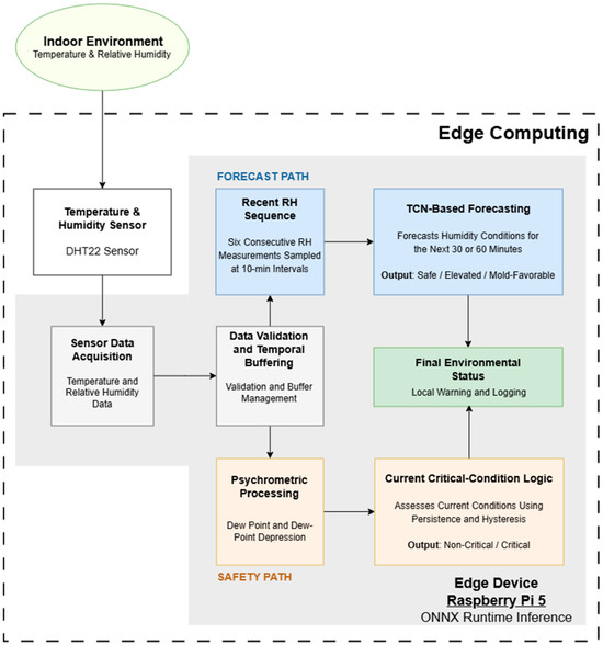
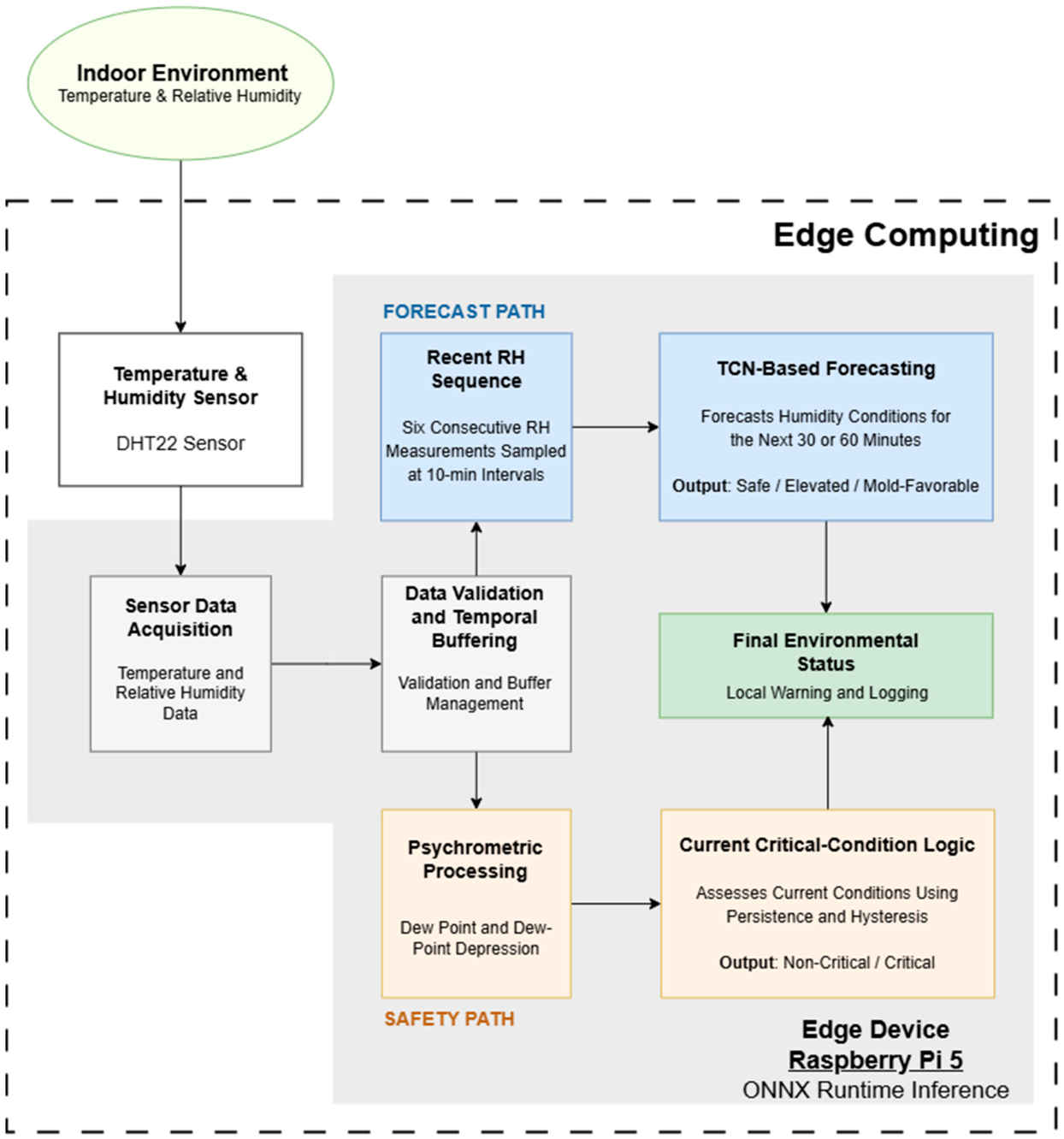
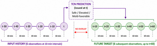
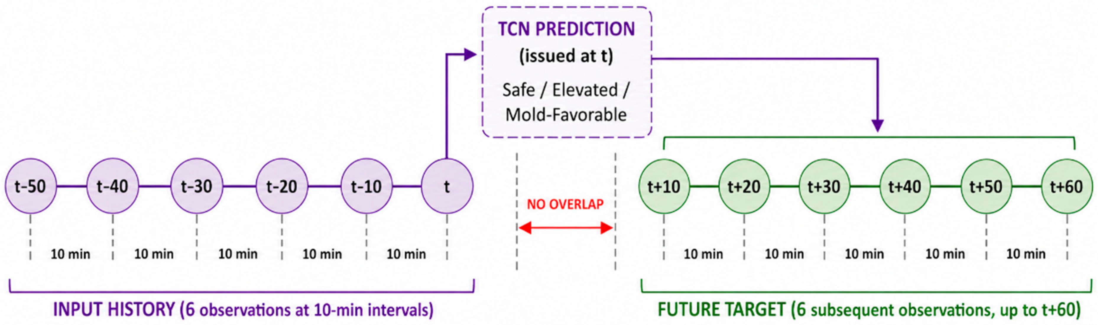
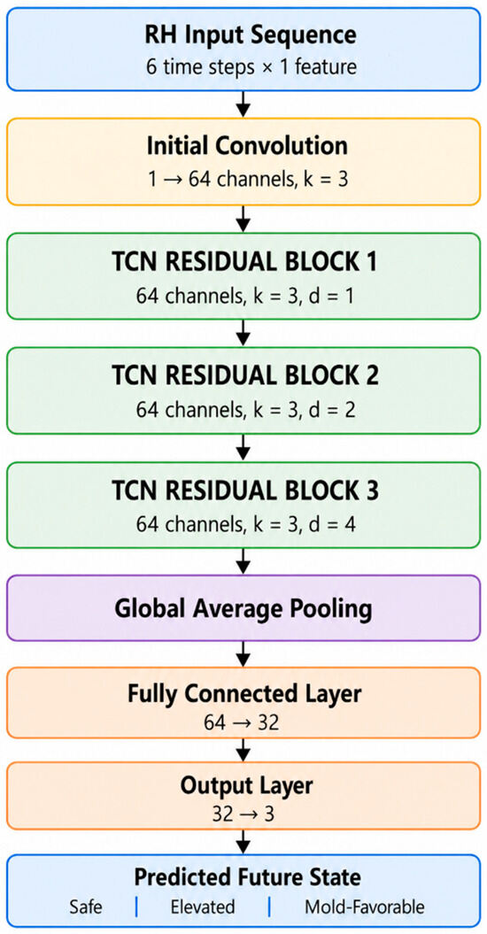
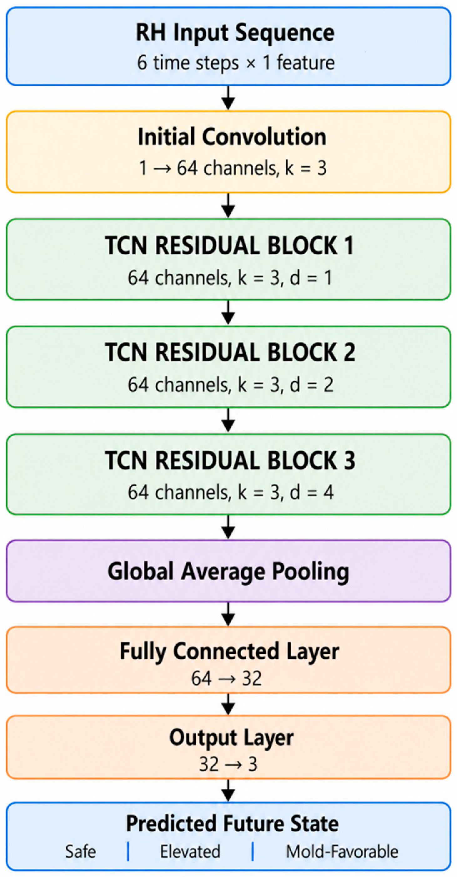
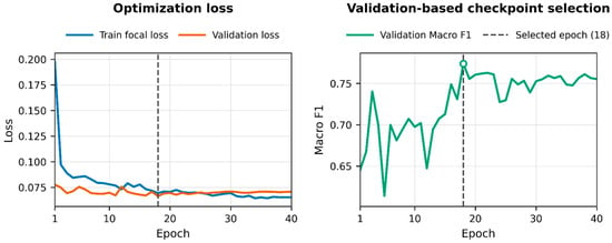
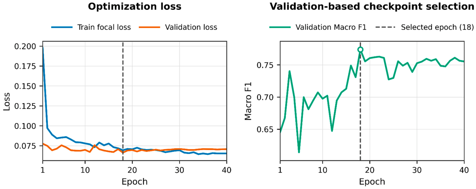
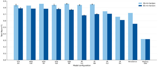
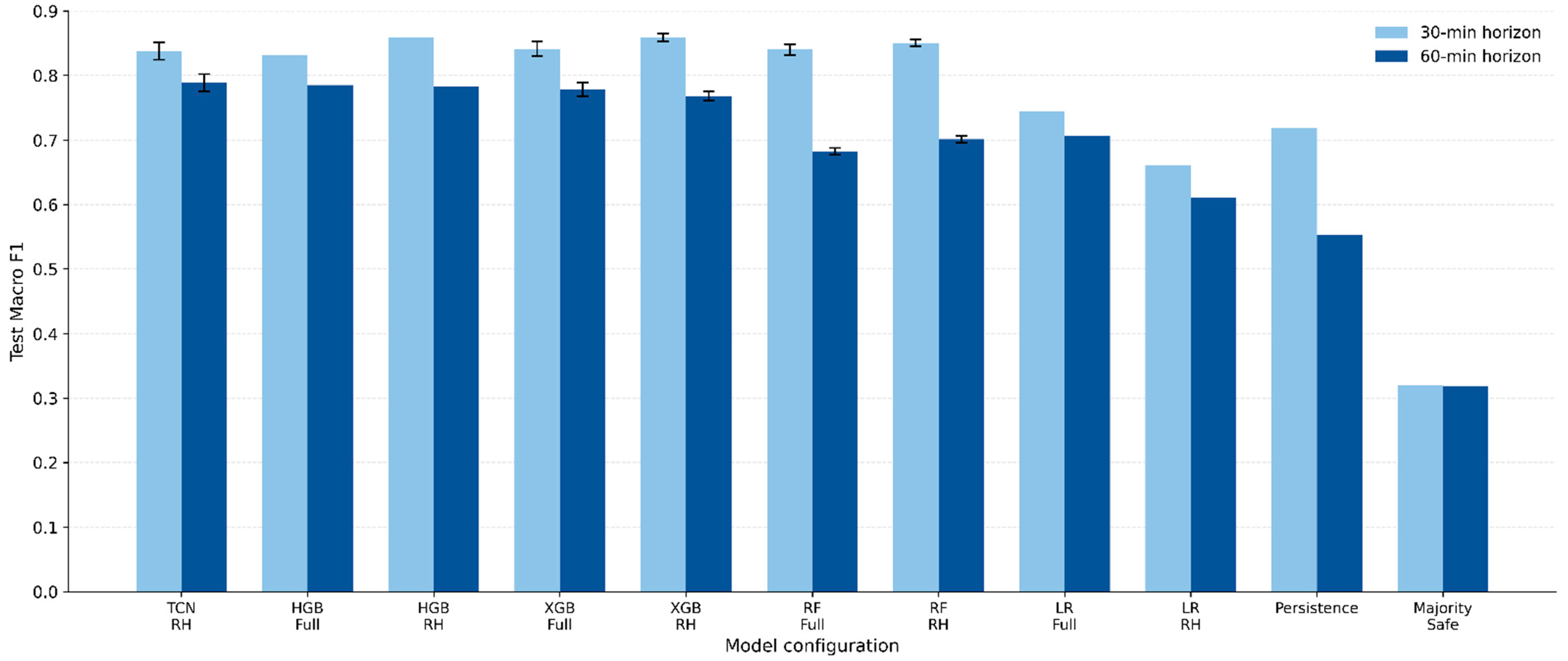
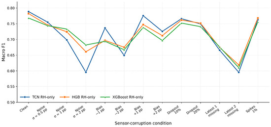
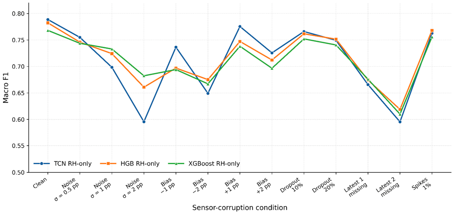
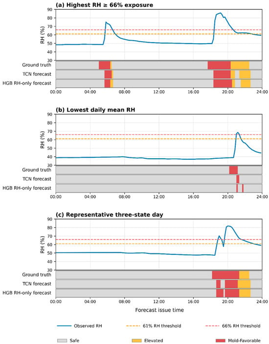
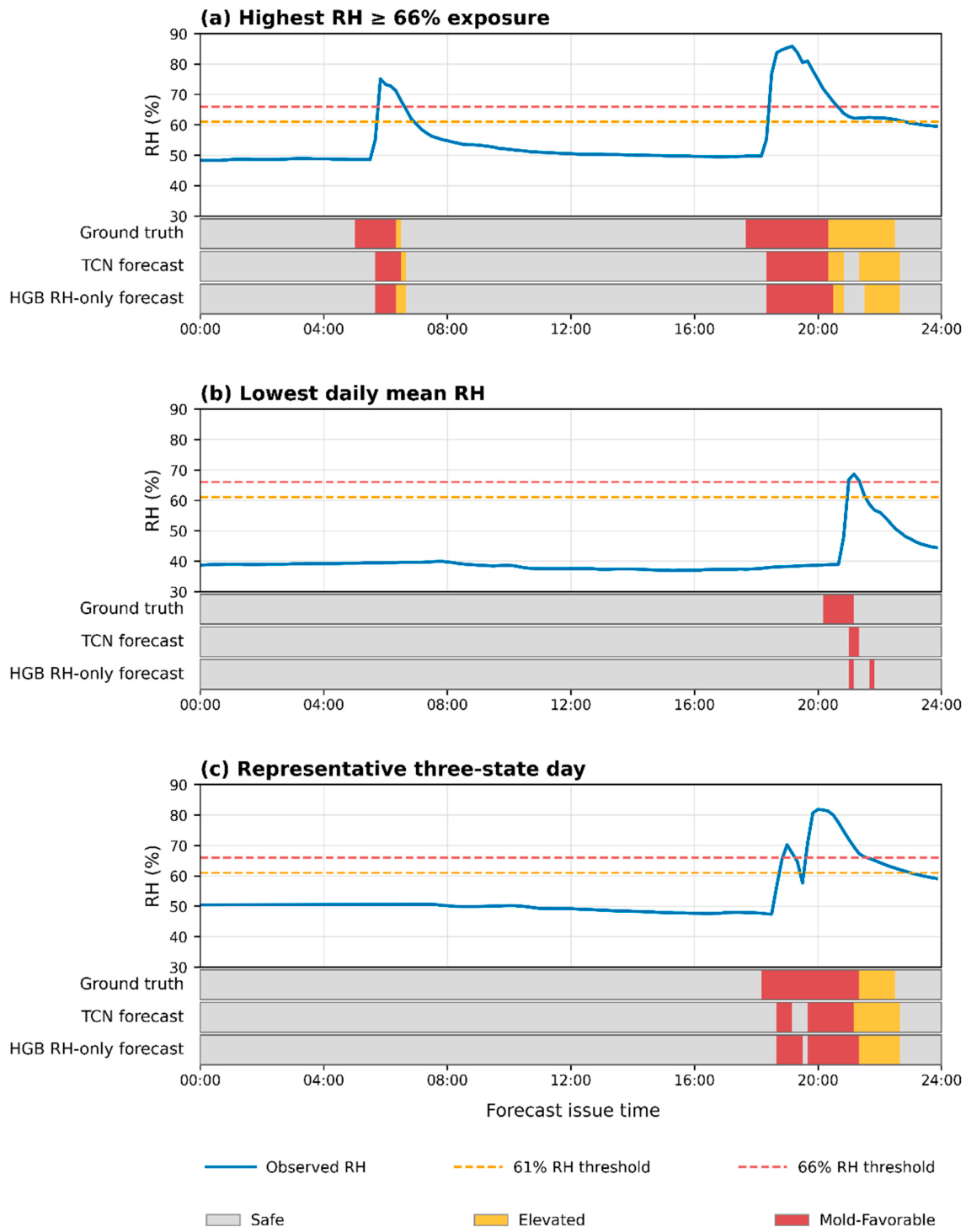
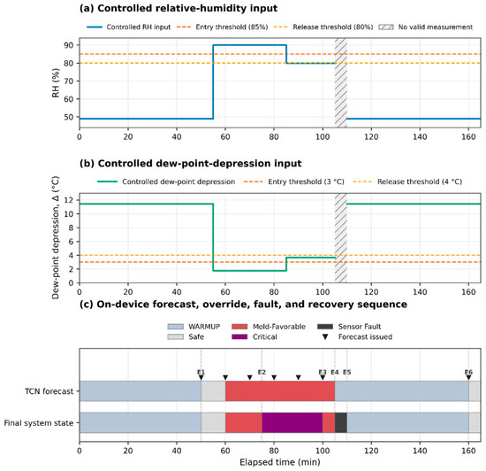
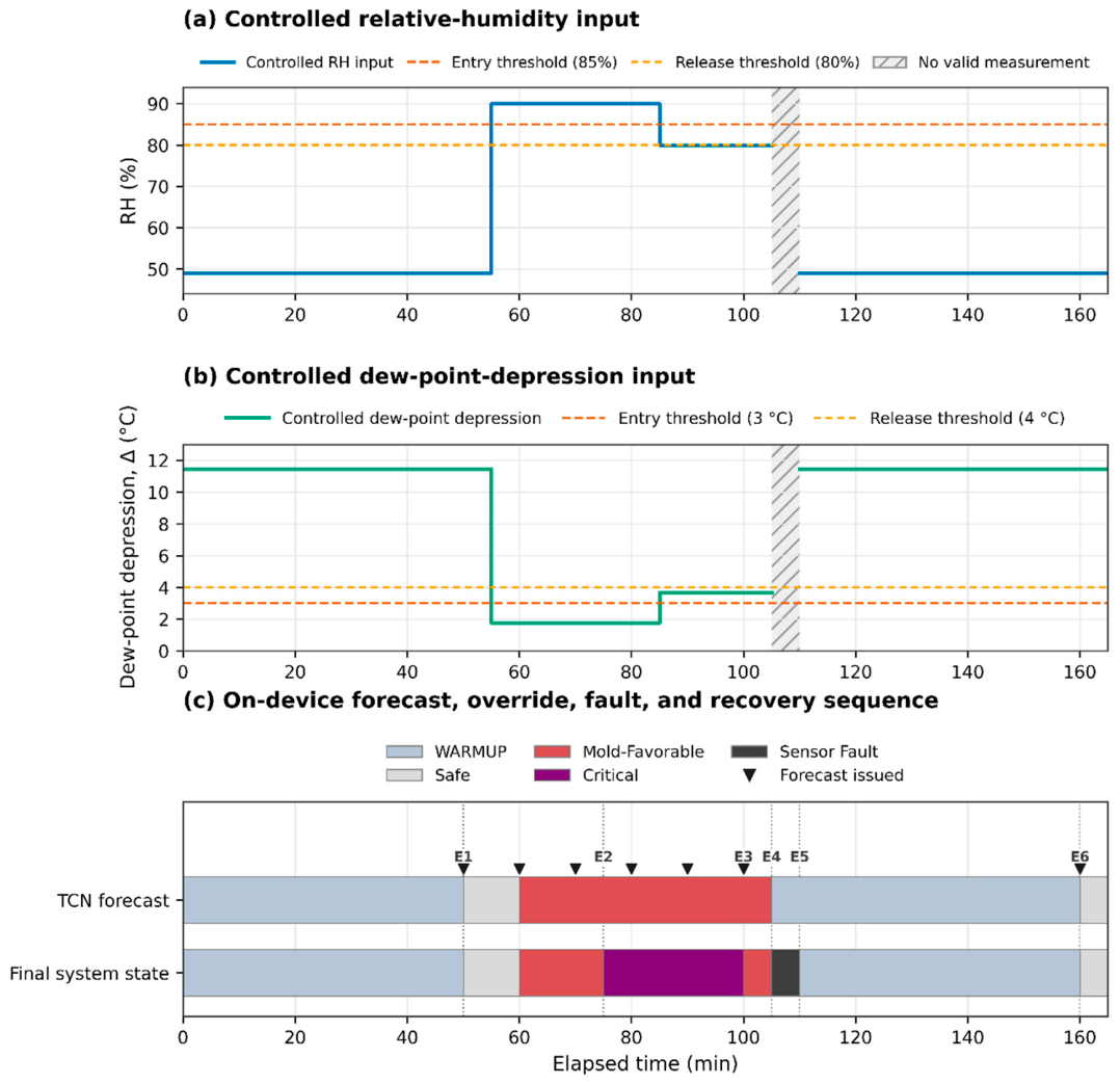

Disclaimer/Publisher’s Note: The statements, opinions and data contained in all publications are solely those of the individual author(s) and contributor(s) and not of MDPI and/or the editor(s). MDPI and/or the editor(s) disclaim responsibility for any injury to people or property resulting from any ideas, methods, instructions or products referred to in the content. |
© 2026 by the authors. Licensee MDPI, Basel, Switzerland. This article is an open access article distributed under the terms and conditions of the Creative Commons Attribution (CC BY) license.