


Abstract
Automated alert triage can reduce Security Operations Center (SOC) workload, yet the validation-tuned thresholds deployed systems rely on carry no finite-sample control of their operational error rates and degrade unpredictably under distribution shift. We present a model-agnostic dual-threshold conformal deferral architecture: high-score alerts are auto-escalated under finite-sample marginal class-conditional control of the benign-escalation probability (budget α), low-score alerts are auto-closed under matching control of the threat-miss probability (budget β), and the rest are deferred to an analyst. It needs no retraining and closes an automatic zone rather than certifying what the calibration data cannot support. We evaluate it on a reinforcement-learning investigation agent in a simulated SOC and on four classifiers trained on CIC-IDS2017 and tested on CSE-CIC-IDS2018, using stratified 25,000-flow calibration and evaluation samples, with attack-type recall computed over the full 16.2-million-flow corpus. Pooling episodes from ten trained policies across two evaluation datasets, the architecture automated 73.7% of decisions at α = β = 0.01—a figure for that predefined pooled mixture rather than a per-policy or per-dataset guarantee—realizing benign auto-escalation and threat auto-close rates of 0.0099 and 0.0101 and deferring the hardest ~26% of alerts. After recalibration on labeled target-domain data, severe cross-dataset degradation appears not as a silent error but as sharply reduced certifiable automation, with deferral rising to 79–99% for the most affected classifiers. This visibility is a property of the recalibrated layer: thresholds left un-recalibrated after a shift continue to certify nothing while still deciding, so the architecture requires periodic recalibration on labelled target-domain alerts to deliver it. Substituting open-weight language models for the analyst inside the band failed a pre-specified criterion at every scale tested from 7B to 32B across two model families, with the discriminative signal flat in model size and far below the first-stage policy’s own.
1. Introduction
Security Operations Centers (SOCs) receive far more alerts than their analysts can review. Surveys of practitioner workload consistently report that the majority of alerts reaching a Tier-1 queue are false positives and that a substantial fraction is never examined at all [1,2]. The operational consequence is not merely wasted effort: alert fatigue degrades the quality of the reviews that do happen, and unreviewed alerts are, in effect, silently closed by the queue rather than by a decision [3]. This is the problem that automated triage is meant to solve, and a large body of work now applies supervised classifiers, anomaly detectors, and, more recently, reinforcement-learning agents and large language models to the task of deciding which alerts deserve an analyst’s attention [4,5,6].
Deploying such a system, however, requires answering a question that most of the literature leaves implicit: how much of the queue can safely be automated, and at what error rate? In practice, the answer is usually a threshold—escalate above it, close below it—chosen on a validation set and held fixed. Two properties of that arrangement are uncomfortable for a security team: the threshold carries no finite-sample guarantee, and it forces a binary decision even on the alerts whose score carries almost no information, silently and with the same confidence it applies to the easy cases.
The second failure is aggravated by distribution shift, which is the normal condition of a deployed detector rather than an exceptional one. Attack tooling changes, the monitored network changes, and a model trained on last year’s traffic score this year’s traffic differently. A fixed threshold does not notice; it continues to escalate and close at the same cutoff, and the errors it makes are absorbed into the queue without a signal. Our own experiments illustrate how sharply this can bite: models trained on CIC-IDS2017 and evaluated on CSE-CIC-IDS2018 lose detection in a pattern that neither in-distribution accuracy nor a seen/unseen attack taxonomy predicts—the strongest in-distribution model is among the weakest after the shift, and the largest attack class in training is detected perfectly by one model and not at all by another.
This study takes a different position on what triage automation should promise. Rather than deciding every alert, the system should decide only the alerts it can decide with a stated error budget and route the rest to a human. We instantiate this as a dual-threshold conformal deferral architecture: two thresholds, calibrated by split conformal prediction on held-out benign and threat alerts, partition the score range into an auto-escalation zone carrying a finite-sample bound on the benign escalation rate (at most α), an auto-close zone carrying a bound on the automatic miss rate on threats (at most β), and a deferral band in between, which is handed to an analyst. The layer sits on top of an existing scoring model, requires no retraining, and—a property we consider essential rather than incidental—never emits a threshold it cannot certify. When the calibration data are insufficient to support a requested budget, the corresponding zone closes, and its alerts are deferred, instead of a heuristic cutoff being substituted.
The statistical machinery we use is standard [7,8], and so are its ingredients, as assembled here. It consists of split (inductive) conformal prediction applied class-conditionally: the calibration alerts of each class are scored by the unmodified detector, the scores are sorted, and a single order statistic of each sorted list becomes a threshold—the ⌈(1 − α)(nb + 1)⌉-th of the benign scores and the ⌊β(nt + 1)⌋-th of the threat scores. Exchangeability between calibration and deployment alerts within a class is what makes the resulting tail probabilities’ finite sample valid without any distributional assumption, and the fact that the construction touches only the score, never the model, is what makes it a wrapper. There is no learning, no optimization, and no free parameter beyond the two budgets. Angelopoulos et al. [9] partition medical-imaging cases into low-risk, high-risk, and uncertain groups by wrapping a black-box model in a conformal procedure. Garcia et al. [10] choose class-conditional conformal cutoffs that bound the false-positive and false-negative rates of a clinical risk score. PAC-Wrap [11] endows an arbitrary anomaly detector with PAC bounds on both error rates. CRC-SGAD [12] applies dual-threshold conformal risk control to graph anomaly detection in a security domain. We, therefore, claim novelty for none of the statistical components individually—not the three-zone geometry, not class-conditional error control, not the second threshold, not the model-agnostic wrapper form. What we contribute is their operationalization for SOC triage and a characterization of what the resulting layer does in deployment. Two design choices define that operationalization. The first is which risks the budgets name: where conformal triage certifies predictive values, which move with the prevalence of threats in the queue, our thresholds certify class-conditional error rates, which do not. An operator can, therefore, set a tolerance for wasted incident response effort and one for missed threats once, before deployment, rather than requalifying them whenever the queue composition drifts. Section 3.4 develops the argument, and Section 8.2 exhibits the invariance. The second design choice is what the layer does when it cannot certify: it closes the corresponding zone rather than substituting an uncertified cutoff, and Section 5.4 measures what that choice is worth. The rest of what we offer is empirical.
We formulate SOC triage as a selective automation problem with two independent, operator-chosen, prevalence-invariant error budgets, and specify a deferral architecture that is model-agnostic, training-free, and explicit about infeasibility (Section 3).
We evaluate it on two independent evidence lines—a reinforcement-learning investigation agent in a simulated SOC and four conventional classifiers on real intrusion detection data (CIC-IDS2017/2018, 16.2 M flows)—and show that the amount of automation is an output of calibration rather than a design constant: at α = β = 0.01, the architecture automated 73.7% of decisions under the pooled hardened-regime protocol, where thresholds are calibrated on episodes pooled across ten trained policies and shared across both evaluation datasets—the figure characterizes that mixture and does not transfer unchanged to an individual policy or a single dataset, as the seed-level analysis of Section 5.1 shows—and degenerates gracefully to full automation when the base model is strong enough not to need help (Section 5).
We identify and quantify a selection effect that determines what is deferred and why single-threshold gates pay for false-positive control with structural recall loss: the escalated-benign alerts on which any such gate must calibrate lie close to the threat distribution, a pattern we observe for the RL agent and for all four classifiers (Section 5.3).
We show that under distribution shift, the architecture fails visibly rather than silently: as detection collapses, the deferral band inflates—from 24% to 88% of alerts for logistic regression, and from full automation to 79–99% deferral for the tree ensembles—turning a hidden loss of detection into measurable analyst workload, without any dedicated drift monitor but only under a periodic-recalibration regime: the inflation is a property of thresholds recalibrated on labelled target-domain alerts, and a layer left on stale thresholds exhibits none of it (Section 6).
We report a negative result for the most natural extension of the architecture—resolving the band with an open-weight language model instead of an analyst, tested at four scales from 7B to 32B across two model families—evaluated against a criterion fixed before the experiment, and analyze why it fails (Section 7).
We also document, in Section 4.1, an evaluation-signal defect discovered during development: an earlier version of our simulation derived the agent’s confidence from a label-conditional monotone accumulator, which made the score a near-perfect proxy for ground truth and inflated every downstream result. We describe the defect, the three checks that expose it, and the correction, because the same trap is available to anyone constructing a simulated triage environment from a static intrusion detection corpus.
The remainder of this paper is organized as follows. Section 2 reviews related work on alert triage, conformal prediction, and selective classification. Section 3 specifies the architecture and its calibration. Section 4 describes the two evidence lines and the evaluation protocol. Section 5 and Section 6 report results in distribution and under shift. Section 7 presents the LLM pilot. Section 8 translates the results into operational guidance, Section 9 states the limitations, and Section 10 concludes.
2. Related Work
This work sits at the intersection of three areas of the literature: automated alert triage in security operations, distribution-free uncertainty quantification via conformal prediction, and selective classification with deferral to a human expert. We review each in turn and then state what the present architecture adds and what it does not.
2.1. Alert Triage and Analyst Workload
The operational case for triage automation is well documented. Vielberth et al. [13] survey SOC structure and identify alert volume and analyst scarcity as structural rather than transient constraints; Tariq et al. [2] review alert fatigue as a research problem in its own right, cataloguing its causes and the interventions proposed against it; and Jalalvand et al. [5] systematize the alert prioritization literature by criteria and method, showing that the dominant formulation is a ranking or scoring problem whose output is consumed by a fixed cutoff.
Methodologically, the field spans provenance-based filtering [3], semi-supervised contextual analysis of event sequences (DEEPCASE [4], which reports automatically filtering 86.7% of events), and, more recently, large language models acting as investigators or multi-agent triage systems [6,14]. What these systems share is the property this study takes issue with: their operating point is selected empirically, and the error rate it will produce in deployment is an estimate rather than a certificate. DEEPCASE, for instance, reports its workload reduction as a quantity measured on the evaluated corpus; nothing in the construction bounds the rate at which it will discard true threats elsewhere. Our contribution is orthogonal to these detectors rather than competitive with them: the deferral layer consumes whatever score they produce, and Section 4 exercises it on two deliberately different ones.
2.2. Conformal Prediction and Distribution-Free Guarantees
Conformal prediction [7,8] turns a black-box score into a decision rule with finite-sample validity under exchangeability, with no retraining and no distributional assumptions. The split (inductive) variant [15,16] achieves this at the cost of a single held-out calibration pass, which is what makes it deployable as a wrapper around an existing model. The framework has since been extended from coverage to general risk control [17,18], and its exchangeability requirement has been relaxed in specific directions: weighted conformal prediction under known covariate shift [19], and non-exchangeable conformal prediction with a bounded coverage penalty [20]. We use none of these extensions—our thresholds are plain order statistics—but Section 6 recalibrates on target-domain labels precisely because the shift we study violates exchangeability in a way these extensions would not by themselves repair.
The closest prior construction is the conformal triage algorithm of Angelopoulos et al. [9], which partitions patients into low-risk, high-risk, and uncertain groups by wrapping a black-box medical-imaging model in a conformal procedure, post hoc and without retraining. The three-zone geometry is the same as ours, and we claim no priority over it. Two differences are material for the security setting. First, the guarantees differ in kind: conformal triage certifies predictive values—a high positive predictive value in the high-risk group, a high negative predictive value in the low-risk group—which are prevalence-dependent quantities, whereas our thresholds certify class-conditional error rates, the fraction of benign alerts that are auto-escalated and the fraction of threats that are auto-closed. These are the quantities a security team budgets against, and, unlike predictive values, they do not move when alert prevalence moves. Second, we make infeasibility an explicit part of the decision semantics (Section 3.3): when the calibration pool cannot support a requested budget, the zone closes rather than being backfilled by a heuristic cutoff, and Section 5.4 measures what the alternatives cost. Beyond these, what we add is a characterization of how such a layer behaves in security triage—what it defers and why (Section 5.3), how it responds to detector collapse under shift (Section 6), and whether a second automated stage can resolve the band (Section 7).
2.3. Selective Classification and Learning to Defer
Abstention is an old idea. Chow [21] characterized the optimal error–reject tradeoff under a known posterior, and the modern selective classification literature [22,23] studies how to recover a comparable tradeoff from a learned model with an unknown one. Learning to defer generalizes this by modeling the downstream expert explicitly, either to improve fairness and accuracy jointly [24] or through consistent surrogate losses that account for the expert’s own error profile [25]. Straitouri et al. [26] approach the intersection from the opposite direction, using conformal prediction sets to restrict the options presented to a human decision maker rather than to decide whether to present the case at all.
Within security, Jalalvand et al. [27] apply learning to defer to SOC alert prioritization and extend it with human feedback, using deep reinforcement learning to adapt the deferral policy over time. That work and ours address the same operational problem with opposite tradeoffs, and the contrast is the cleanest way to state our position. L2DHF learns a deferral policy: it can, therefore, improve with experience and exploit analyst-specific competence, but the resulting policy carries no finite-sample error bound and requires training data and a live feedback channel. Our layer learns nothing at all. It applies two order statistics to a held-out calibration pool, and in exchange it states an error budget it can certify and refuses to state one it cannot. The two are complementary rather than exclusive; wrapping a learned deferral policy in a certified outer envelope is a natural direction that we do not pursue here.
2.4. Uncertainty Quantification and Generalization in Intrusion Detection
Uncertainty quantification has begun to reach network intrusion detection [28], but the failure mode that dominates the empirical literature there is not in-distribution miscalibration: it is the collapse of detection across networks. The CIC corpora [29] on which much of this work rests carry documented labeling and flow construction defects [30], and cross-dataset evaluation consistently reports that near-perfect in-distribution accuracy does not survive a change of network [31,32,33]. Arp et al. [34] place these findings within a broader catalogue of methodological pitfalls in security machine learning. Section 6 reproduces this collapse rather than contesting it. Our claim there is not the observation that transfer fails, which is established, but the demonstration that a conformal deferral layer converts that failure from silent error into visible workload, with no drift monitor attached.
2.5. Positioning
Taken together, the work reviewed above establishes each statistical ingredient of the layer we describe. Three-zone conformal triage is established [9]; class-conditional conformal control of the false-positive and false-negative rates is established [10]; two-sided error-rate bounds around an arbitrary black-box detector are established [11]; and dual-threshold conformal risk control has already been applied in a security domain [12]. We, therefore, make no claim of novelty for any of these components in isolation, and a reader looking for a new conformal method will not find one here. Table 1 sets out what each of the four closest works controls and where the present system differs.
Table 1.
The four closest prior constructions, the risk each controls, and what the present architecture adds. The differences are operational rather than statistical; the statistical components are shared.
Our contribution is the assembly and its empirical characterization for security operations: two budgets that name the two errors an SOC actually trades against each other; fail-safe semantics that close a zone rather than certify what the calibration data cannot support; evaluation of one unchanged layer over two scoring models that share nothing else; a measurement of which alerts the band inherits and why; the behavior of certified automation when a detector collapses across networks; the translation of all of it into alerts per thousand and residual risk; a negative result for the obvious second automated stage; and an evaluation-signal defect we found in our own simulator and report so that others can test for it. None of this follows from the statistical components, and none is reported in the four works above.
3. Dual-Threshold Conformal Deferral Architecture
This section specifies the layer. Section 3.1 fixes the decision rule and the three zones it induces; Section 3.2 gives the two order statistics that calibrate its thresholds and the two assurances they carry; Section 3.3 states what the layer does when the calibration data cannot support a requested budget, which we treat as part of the decision semantics rather than as an error condition; and Section 3.4 bounds what the assurances claim. A reader familiar with split conformal prediction will find no unfamiliar statistics here and may prefer to read Section 3.3 and Section 3.4 alone.
3.1. Problem Setting and Decision Rule
We consider an automated triage system that processes security alerts and, for each alert x, produces a scalar confidence score s(x) ∈ [0, 1], where higher values indicate stronger evidence that the alert corresponds to a true threat. The architecture treats the scoring model as a black box: in our experiments, the score is produced either by a reinforcement-learning investigation policy that accumulates evidence over a multi-step investigation episode (Section 4.1) or by the predicted threat probability of a conventional flow classifier (Section 4.2). No assumption is made about how the score was trained, and the underlying model is never retrained or modified.
Rather than converting the score into a binary escalate/close decision with a single threshold, the architecture partitions the score range into three zones using two calibrated thresholds θlow < θhigh (Figure 1):
Figure 1.
The dual-threshold conformal deferral layer, drawn to show its decision semantics rather than its statistics. The calibration path (left) consumes labelled alerts of each class and returns two order statistics or returns infeasible for a zone whose class pool is too small for the requested budget, in which case that zone closes and its alerts join the band rather than being decided by an uncalibrated cutoff. The scoring path (right) is unmodified: the layer adds two scalar comparisons and no model. The band is drawn as an output with a cost attached, because that is how the architecture is meant to be budgeted. The statistical components are standard and are attributed in Table 1; what this figure depicts, and what the paper contributes, is their arrangement into a triage decision rule with an explicit failure mode.
AUTO-ESCALATE: if s(x) > θhigh, the alert is escalated to incident response without human review.
AUTO-CLOSE: if s(x) < θlow, the alert is closed as a false positive without human review.
DEFER: if θlow ≤ s(x) ≤ θhigh, the alert is routed to a human analyst, who makes the final decision.
In Figure 1, a black-box triage model (an RL investigation policy or a flow classifier) produces a confidence score, which is partitioned into three zones by two conformally calibrated thresholds. Alerts above θhigh are auto-escalated (benign auto-escalation rate ≤ α); alerts below θlow are auto-closed (threat auto-close rate ≤ β); alerts in the band are deferred to a human analyst. If calibration is infeasible, the corresponding automatic zone closes; if the band is empty, the system degrades to full automation.
The design goal is operational: the two automatic zones carry explicit, user-selected error budgets, while the alerts on which the system cannot make a certified decision are exactly the ones placed in front of the analyst. The two budgets are asymmetric by construction, reflecting the asymmetric costs of triage errors: α bounds the rate at which benign alerts consume analyst and incident response effort through automatic escalation, and β bounds the rate at which true threats are silently discarded by automatic closure.
3.2. Threshold Calibration
Both thresholds are obtained by split-conformal calibration on held-out labeled alerts, using the full benign and threat calibration pools rather than any policy-selected subset. Let b = {x:y(x) = benign} and t = {x:y(x) = threat} denote the benign and threat calibration sets, of sizes nb and nt, and let
be the corresponding scores sorted in ascending order. Given an escalation budget α ∈ (0, 1) and a miss budget β ∈ (0, 1), the two thresholds are the order statistics
and, provided θlow < θhigh, the decision rule of Section 3.1 is applied with strict inequalities:
The two rounding directions are not a stylistic inconsistency: each is the choice that makes its own bound conservative. Equation (2) bounds an upper-tail probability, so the index must be rounded up—taking the ⌈(1 − α)(nb + 1)⌉-th order statistic places the threshold at or above the exact quantile and admits at most α of the benign mass. Equation (3) bounds a lower-tail probability, so the index must be rounded down—taking the ⌊β(nt + 1)⌋-th order statistic places the threshold at or below the exact quantile and admits at most β of the threat mass. Rounding either the other way would move the threshold across the exact quantile and forfeit the finite-sample guarantee. The same asymmetry is what makes the feasibility conditions of Equation (7) differ in form: the upper threshold fails to exist when the ceiling exceeds nb, the lower when the floor falls below 1. Strict inequalities preserve conservative validity in the presence of ties, which arise here because mass accumulates at the clipping bounds (Section 4.1). Replacing s > θhigh with s ≥ θhigh would add the entire probability mass at the threshold to the automatic zone and can violate the nominal bound unless randomized tie-breaking or a no-ties assumption is imposed.
Equations (2) and (3) are standard split-conformal constructions [7,8,15]. When the calibration and deployment alerts of a given class are exchangeable, they yield the two assurances the architecture is built on:
Both statements hold in expectation over the draw of the calibration set; realized rates on any single deployment sample fluctuate around the targets, and we, therefore, report realized rates (, ) alongside the nominal budgets throughout the evaluation. We emphasize that the guarantees concern the automatic zones only: nothing is claimed about the quality of decisions made on deferred alerts, which is precisely why those alerts are routed to a human.
A threshold exists only if its order statistic is defined: the upper zone is feasible when the benign pool satisfies
For α = β = 0.01, this requires at least 99 calibration alerts of each class; when either condition fails, the corresponding zone is infeasible and closes (Section 3.3).
The two thresholds are calibrated independently, and nothing constrains their order: when the benign and threat score distributions are separated more sharply than the requested budgets demand, the calibration returns θlow ≥ θhigh and the two automatic zones overlap, leaving Equation (4) undefined on the overlap. In this regime, the overlap is resolved as follows. If θlow > θhigh, the architecture collapses to a single cut at c = θlow,
and the deferral band is empty. Since c > θhigh, the escalation region of Equation (8) is strictly contained in the conformally certified upper region, and the closure region is unchanged, so both bounds are preserved. If θlow = θhigh = c, alerts tied exactly at c are deferred, since neither strict condition of Equation (4) certifies them; assigning this tie mass automatically would require randomized tie-breaking or a no-ties assumption. This is precisely the behavior of our implementation, in which the two strict comparisons of Equation (4) are applied in sequence and unclaimed alerts remain deferred. Crossing is, therefore, not a failure of calibration but a signal that certified automation is available across essentially the entire score range; we observe it in the standard RL regime at most budgets and in the hardened regime at loose ones (Section 5.2).
3.3. Feasibility, Degeneration, and Fallback Semantics
A conformal threshold exists only when the calibration pool is large enough for the requested budget: the upper threshold requires ⌈(1 − α)(nb + 1)⌉ ≤ nb, which for small α translates into a minimum number of benign calibration alerts (for example, α = 0.01 requires nb ≥ 99). When this condition fails, the architecture does not fall back to a heuristic threshold. Instead, the corresponding automatic zone is declared infeasible and closed, and the alerts that would have entered it are deferred. The same rule applies independently to the lower threshold. This is a deliberate design choice, motivated by our calibration-reliability results (Section 5.4): alternatives such as validation-tuned thresholds will readily produce a cutoff from a handful of examples, silently voiding any error control.
Two degenerate configurations arise naturally and are handled without special cases. First, if the calibrated thresholds cross strictly (θlow > θhigh), the deferral band is empty and the system operates as a fully automatic two-zone policy; if the two coincide, only alerts whose score ties the common threshold remain deferred (Section 3.2). We observe this when the base model is already highly accurate and the score distributions are well separated. Second, if both thresholds are infeasible, every alert is deferred and the system degrades to fully manual triage. In neither case does the architecture fabricate a certificate it cannot support; the amount of automation offered is itself an output of calibration, not a fixed promise.
3.4. Scope of the Guarantees
Three boundaries of the assurance statements deserve explicit mention, since they shape how the architecture should be operated. First, the guarantees are marginal: they hold on average over calibration randomness, not conditionally on every subpopulation of alerts. Second, they are class-conditional error bounds for the automatic zones, not end-to-end performance claims; overall system performance additionally depends on how deferred alerts are resolved, which we quantify operationally in Section 8. Being class-conditional is precisely what makes them prevalence-invariant: Equations (5) and (6) condition on the true class, so each bound depends only on the score distribution within that class and not on the proportion in which the two classes are mixed. Holding the within-class score distributions fixed, the same calibrated thresholds, therefore, carry the same α and β whether 5% or 50% of the queue is a real threat. The invariance is to the mixing proportion alone; it is not invariance to arbitrary distribution shift, which moves the within-class distributions themselves and is the subject of Section 6. This is what separates them from predictive-value certificates [9], which the same thresholds yield only once a prevalence is fixed, and it is why the budgets can be set once rather than requalified as the queue composition drifts. The cost of the choice deserves equal billing: our bounds say nothing about the positive or negative predictive value an analyst or an incident responder will actually experience, and those quantities do move with prevalence. Third, the guarantees require exchangeability between calibration and deployment alerts within each class; they do not require the model-training distribution to match the deployment distribution. Section 6 studies a training-to-target shift while recalibrating the thresholds on labeled target-domain alerts and evaluating on a disjoint target-domain split, so the resulting guarantees pertain to that target-domain operating period; subsequent drift between calibration and deployment is not covered.
4. Experimental Setup
We evaluate the architecture on two independent evidence lines that share nothing except the deferral layer itself: a reinforcement-learning investigation agent operating in a simulated SOC environment and four conventional classifiers scoring real network flows across a dataset shift. The purpose of this design is to demonstrate that the architecture’s behavior—calibrated automation, abstention under infeasibility, and band inflation under shift—is a property of the deferral layer rather than of any particular scoring model.
This section describes the two evidence lines and the protocol that governs both. Section 4.1 covers the reinforcement-learning line, including an evaluation-signal defect we found in our own simulator and the checks that expose it; Section 4.2 covers the cross-dataset flow classifiers and the feature harmonization they require; Section 4.3 states the calibration and evaluation protocol, whose exchangeability properties matter for how the results in Section 5 should be read.
4.1. RL Evidence Line: Simulated SOC Investigation
The first evidence line uses a PPO agent [35] (Stable-Baselines3 1.8.0 [36]) that investigates episodes drawn against labels from the CIC-IDS2017, CSE-CIC-IDS2018 [29], and UNSW-NB15 [37] corpora. Each episode corresponds to one alert. The agent observes a 256-dimensional state encoding investigation progress, indicator-of-compromise (IoC) counts, threat intelligence (CTI) match status, MITRE ATT&CK [38] technique coverage, and the running confidence estimate, and chooses among five discrete actions: three evidence-gathering actions (querying additional logs, investigating lateral movement, querying a CTI feed) and two terminal actions (escalate, close as false positive). Evidence gathering updates a scalar confidence variable through stochastic increments whose distributions depend on the underlying ground truth of the alert but overlap across classes: evidence collection can fail for true threats (decreasing confidence) and can spuriously succeed for benign alerts (increasing it). Confidence is clipped to [0.02, 0.98]. Rewards are assigned against ground truth only at episode termination (+1.0 for a correct escalation, −2.5 for a false escalation, +1.5 for a correct close, −2.0 for a missed threat), complemented by a small decision bonus, a growing per-step cost, and a timeout penalty that discourage indefinite investigation. The terminal confidence value is the score s(x) consumed by the deferral layer.
What the corpora contribute is narrower than the phrase might suggest, and we state it plainly because the alternative reading would ascribe more external validity to this evidence line than it has. Each episode is instantiated by drawing a record from the corresponding corpus and taking its ground-truth label—benign or attack, together with the attack type where one applies. Everything the agent subsequently observes is generated by the simulator: the 256-dimensional state encoding, the IoC and CTI events, the MITRE technique matches, and the stochastic confidence increments are produced by the environment’s own generative process, conditioned only on that label and on the regime parameters. The flow features themselves are never presented to the agent, and no per-flow characteristic other than the label influences the episode. The technical difference between a CSE-CIC-IDS2018 episode stream and a UNSW-NB15 one is, therefore, confined to two things: the threat prevalence of the draw (30% and 56%, respectively, in the hardened regime) and the attack-type composition behind the positive labels. The evidence dynamics are identical, and the cross-corpus contrast this line supports is a contrast of label mixtures, not of network behavior; the real-data evidence line of Section 4.2, where the classifiers consume actual flow features, is what carries the cross-network claims. Agents are trained for 106 timesteps per run and evaluated on episodes drawn against labels from CSE-CIC-IDS2018 and UNSW-NB15, with ten independent training seeds per regime and 200 evaluation episodes per seed and dataset. We evaluate two regimes. In the standard regime, evidence is comparatively informative and the trained policy is already conservative. In the hardened regime, stealthy threats initialize at a confidence drawn uniformly from [0.30, 0.55] and evidence increments are damped by a factor of 0.5, producing substantially harder episodes; this is the regime in which the deferral band is exercised.
Validation of the simulation signal
An earlier version of this environment contained a defect that we report because it is easy to reproduce in any simulated triage environment and because it silently invalidates evaluation: confidence increments were deterministic in sign conditional on ground truth—every action increased confidence for threats and decreased it, on average, for benign alerts. The confidence signal was, therefore, a monotone accumulator of the label itself: every threat episode terminated at a confidence of exactly 1.0 (zero variance), and any threshold-based mechanism evaluated on this signal appeared to achieve perfect recall at arbitrary false-positive targets. We detected the defect with three checks that we recommend as a standard validation step for simulated triage environments: (i) label-conditional monotonicity—testing whether the sign of the score increment is deterministic given the label; (ii) saturation statistics—per-class unique-value counts, standard deviations, and boundary-mass fractions of the terminal score; and (iii) a separability upper bound—flagging environments in which the score is a perfect classifier (class overlap ≈ 0). The corrected environment described above passes check (i); check (ii) still reports substantial threat-class mass at the 0.98 ceiling (35–55% depending on regime and dataset), a residual, weaker form of conditional drift that we report in Table 2 and account for in Section 10. All results in this study are produced with the corrected environment; no result from the defective version is used.
Table 2.
Terminal confidence statistics of the simulation signal before and after correction of the oracle confidence defect. Corrected-version cells report CSE-CIC-IDS2018/UNSW-NB15 values separately; defective-version statistics are pooled across datasets. In the defective version, the signal is a deterministic function of the ground-truth label (zero threat-class variance).
4.2. Real-Data Evidence Line: Cross-Dataset Flow Classification
The second evidence line uses no reinforcement learning and no simulation. We train four standard classifiers—XGBoost [39], random forest, a multilayer perceptron, and logistic regression, each with a fixed hyperparameter configuration chosen before any evaluation and never tuned against a test set (the exact settings are listed in Appendix A)—on flows from CIC-IDS2017 and evaluate them both in distribution and under a realistic dataset shift to CSE-CIC-IDS2018. The two corpora are produced by the same feature extractor (CICFlowMeter [29], whose known labeling and flow construction caveats are documented in [30]) but with divergent column naming; we align them with a mechanical harmonization procedure (name normalization followed by token-order-invariant matching) that yields 74 matched feature pairs. From these, we drop 13 that correspond to identifiers or flow-level bookkeeping rather than traffic characteristics (the label, destination port, and aggregate flow/subflow timing and volume fields) and a further 4 that are constant in the training corpus, leaving 57 features. The harmonization map, the excluded fields, the constant-feature list, and an attack-type correspondence table (including spelling variants such as Infilteration/Infiltration) are released with the code. An analogous harmonization against UNSW-NB15 does not produce a usable common feature set, owing to a structurally different extractor; the incompatibility report is included in the repository, and the real-data line, therefore, uses the CIC pair only.
Training uses a stratified sample of 100,000 flows from CIC-IDS2017; in-distribution evaluation uses a disjoint 25,000-flow holdout. The cross-dataset corpus is the complete ten-day CSE-CIC-IDS2018 release (16.2 M flows, fourteen attack types); calibration and permutation-based evaluation use a stratified 25,000-flow sample that preserves attack-type proportions, and type-level detection rates are additionally computed by scoring the full corpus. The classifier’s predicted threat probability serves as the score s(x), and its default 0.5 operating point defines the base decision used for reference comparisons. Table 3 summarizes both evidence lines and the operating points of the base models; the collapse of cross-dataset recall visible there (e.g., random forest at 0.010) is analyzed in Section 6.
Table 3.
Summary of the two evidence lines and base-model operating points. RL rows report mean ± standard deviation across ten training seeds; real-data rows report single-run values at the classifier’s default 0.5 operating point. Threat prevalence is rounded to the nearest percent.
4.3. Metrics and Protocol
Calibration-reliability experiments (Section 5.4) additionally use bootstrap resampling with replacement from the benign calibration pool at sizes nb ∈ {25, 50, 100, 250, 500} with 1000 resamples and report the conditional overshoot—the fraction of resamples in which the realized conditional pass-rate exceeds its budget—against the continuous-score reference of Equation (9). In the real-data line, the resamples are drawn from the benign half of the calibration split, and the realized rate is measured on the disjoint benign evaluation half. In the RL line of Section 5.4, the calibration and evaluation pools are formed from two disjoint groups of five training seeds each, so the two pools are generated by different policies; that section reports what this does to the realized rates, averaging over twenty partitions drawn from the C(10,5) = 252 possible groupings rather than fixing one arbitrarily. This seed-level split is specific to Section 5.4. Everywhere else, the RL evidence line is evaluated on the pooled episodes of all ten policies, split by random index permutation, which is the protocol behind the allocation and realized rates of Table 4; the released ‘table4_partitions.csv’ reports how that table would move under the stricter seed-level split.
Table 4.
Three-zone allocation, calibrated thresholds, and realized automatic-zone error rates for the RL evidence line (means over ten calibration/evaluation permutations; thresholds pooled across seeds and shared across evaluation datasets). Empty bands indicate two-zone operation (Section 3.3).
Under the cross-dataset protocol of Section 6.2, the thresholds are recalibrated inside the shifted domain. The 25,000-flow CSE-CIC-IDS2018 evaluation sample—itself drawn from the full corpus with proportions stratified by attack type—is split by random index permutation into disjoint calibration and evaluation halves of 12,500 flows each. The thresholds are calibrated on the first, every reported quantity is measured on the second, and the procedure is repeated over ten permutations. The permutation is over indices and is not itself stratified; the realized class counts are reported alongside the shift protocol in Section 6.2. No flow contributes to both halves of any permutation, and both class pools exceed the Equation (7) feasibility minimum by more than an order of magnitude, so no zone reported under shift closes for want of calibration data. The baseline of Section 5.4 is the validation-tuned threshold, which we implement as the (1 − α)-th sample quantile of the benign scores in the calibration resample—the empirical cutoff that targets a pass rate of α without the finite-sample correction of Equation (2). It consumes exactly the same resample as the conformal construction, so the two differ only in that correction.
5. Results: Architecture Behavior in Distribution
This section reports what the layer does when the exchangeability its guarantees assume is satisfied. Section 5.1 gives the three-zone allocation and checks the realized rates against their budgets—a check that is methodological rather than operational, for reasons stated there—and then relaxes the assumption to show what a deployment would actually see. Section 5.2 shows the amount of deferral falling out of calibration rather than being set by design. Section 5.3 identifies which alerts reach the band and why. Section 5.4 asks what the calibration itself is worth when labels are scarce.
5.1. Automation, Deferral, and Guarantee Validation
One property of this protocol should be stated before the numbers are read. Calibration and evaluation episodes are drawn by random index permutation of a single pooled set, which makes them exchangeable by construction—the premise of Equations (5) and (6) holds exactly rather than approximately. Agreement between and α in Table 4 is, therefore, a methodological check that the order statistics of Equations (2) and (3) are implemented and applied correctly. It is not evidence about deployment, where calibration and deployment alerts are separated by time, by policy version, or by network; Table 5 relaxes exactly this assumption and reports what happens. A second property of the table is that rows whose permutations do not all realize the same threshold geometry are now reported split by geometry, because a mean over crossed and three-zone permutations averages quantities that are not commensurable—in a crossed permutation, there is no band, and θlow is a single cut rather than a band edge. Table 4 reports the three-zone allocation and the realized automatic-zone error rates for the RL evidence line across representative (α, β) configurations; Figure 2 visualizes the corresponding score distributions and calibrated thresholds in the hardened regime.
Table 5.
Realized rates and allocation under the stricter seed-level split, in which the calibration and evaluation pools are generated by disjoint groups of five trained policies. Statistics are over all C(10,5) = 252 partitions of the ten seeds, per evaluation dataset (504 draws per configuration), hardened regime. The final two columns give the fraction of draws on which the realized rate respects its budget. Unlike Table 4, this protocol does not make calibration and evaluation exchangeable by construction. Per-partition values are released as table4_partitions.csv.
Figure 2.
Terminal confidence distributions in the hardened RL regime with calibrated thresholds (α = β = 0.01, pooled calibration) on (A) CSE-CIC-IDS2018 and (B) UNSW-NB15. The shaded region is the deferral band; band size and composition are annotated.
In the hardened regime at the strictest configuration (α = β = 0.01), the architecture automates 73.7% of all triage decisions—43.4% closed automatically and 30.3% escalated automatically—while deferring the remaining 26.3% to the analyst. The realized rates closely track the nominal targets: the mean benign auto-escalation rate is = 0.0099 and the mean threat auto-close rate is = 0.0101, for nominal budgets of α = β = 0.01. The finite-sample assurance is marginal over the calibration draw and a future alert; it is not a deterministic upper bound on the realized rate of every finite evaluation split, and empirical rates may accordingly fall on either side of the target. The scope of the certificate deserves stating alongside the number rather than only in Section 9: because the RL calibration pool aggregates episodes across ten trained policies and the thresholds are shared across the two evaluation datasets, the reported rates are marginal over that predefined mixture of policies and domains. They do not imply separate validity for any individual policy or for either dataset alone.
Loosening either budget converts deferred alerts into automated decisions in the direction of the loosened budget, and the composition of the band shifts accordingly. At (α, β) = (0.01, 0.01), the deferred alerts are a near-even mixture (48.9% threats); raising β to 0.05 shrinks the band to 16.6% and concentrates it on threats (67.4%), whereas raising α to 0.05 shrinks it to 15.0% and concentrates it on benign alerts (26.3% threats). The band is, therefore, not a fixed set of “hard alerts” but a controllable spillover whose size and composition follow directly from the operator’s declared risk tolerances; Section 8 translates this dial into analyst workload.
5.2. Regime Dependence and Graceful Degeneration
The standard regime illustrates the architecture’s behavior when the base policy is already strong. There, the trained agent is conservative to begin with (base false-positive rate ≈ 0.003, Table 3), the benign and threat score distributions are well separated, and the calibrated thresholds respond accordingly: at six of the nine (α, β) configurations, the thresholds cross in every calibration permutation, the system reduces to the two-zone policy of Equation (8), and the deferral band is empty. At the strictest configuration (α = β = 0.01), the thresholds cross in 4 of 10 permutations, leaving a thin residual band of 4.8% on average, populated almost entirely by benign alerts (2.0% threats). In other words, the amount of deferral is an output of calibration rather than a design constant: when the underlying model does not need help, the architecture converges toward full automation instead of imposing a fixed review burden, and when the model operates in a genuinely hard regime, the band opens up exactly where certified automation is impossible. The same degeneration appears within the hardened regime at loose budgets—at (α, β) = (0.10, 0.10), the thresholds cross and the band closes—confirming that the transition between three-zone and two-zone operation is governed by the budgets and the score geometry, not by the regime label.
5.3. What Is Deferred: The Selection Effect
The deferred alerts are not a random sample of the traffic; they are systematically the alerts on which score-based automation is least trustworthy, and the mechanism behind this is worth making explicit because it also explains why a natural alternative design fails. Consider the benign alerts that a base policy chooses to escalate. These are, by construction, the benign alerts that most resemble threats in the score: Figure 3 contrasts the score distribution of all benign alerts, of escalated-benign alerts, and of threats, for the RL agent and for a real classifier. In the hardened RL regime, benign alerts as a whole barely overlap the threat distribution (overlap coefficient 0.12–0.14 across the two datasets), but the escalated-benign subset overlaps it two- to three-times more strongly (0.31–0.34), with its mean score shifted from 0.24 to roughly 0.66 against a threat mean of 0.86–0.88. The same concentration appears for the flow classifiers on real data (Table 6). Two consequences follow. First, it characterizes the analyst’s workload under the architecture: the deferral band inherits precisely this contested region, which is why the band’s threat prevalence approaches an even mixture at strict budgets (Table 4)—these are alerts for which the score genuinely carries little information. Second, it explains why we calibrate on full class pools rather than on policy-selected subsets (Section 3.2): a single-threshold escalation gate calibrated only on escalated-benign alerts anchors its threshold inside this shifted subpopulation, pushing the cutoff into the threat mass and paying for false-positive control with a large, structural recall loss. The selection effect is model-agnostic—we observe it for the RL agent and for all four classifiers—and it provides a mechanistic explanation for why a deferral zone can be preferable to a single-threshold gate under the evaluated score distributions.
Figure 3.
The selection effect. Distributions of all benign alerts, escalated-benign alerts, and threats for (A) the RL agent (hardened, CSE-CIC-IDS2018) and (B) logistic regression on the CIC-IDS2017 holdout. Escalated-benign alerts concentrate near the threat distribution (overlap coefficients annotated), explaining why band alerts are intrinsically hard.
Table 6.
The selection effect across scoring models: escalated-benign alerts concentrate near the threat score distribution (overlap coefficients; in-distribution contexts). † n < 25 escalated-benign alerts; these two values are qualitative. At this pool size the 100-bin histogram overlap estimator has a standard deviation of roughly 0.03–0.05 and a downward bias of 0.07–0.22, quantified by subsampling the larger pools (released as table6_smalln_diagnostic.csv), so the digits indicate a magnitude and an ordering rather than a measurement. The bias is conservative with respect to the claim this table supports: it understates OVL(BE, T) while leaving OVL(all-B, T), computed on the full benign pool, unaffected, so the true separation between the two columns is at least as large as shown. The selection effect is established by the four rows with n ≥ 54; the two small rows are consistent with it rather than load bearing for it.
5.4. Calibration Reliability at Small Sample Sizes
The abstention rule in Section 3.3—closing an automatic zone rather than backfilling it with a heuristic threshold—is motivated by how threshold calibration behaves when labeled calibration data are scarce, a routine condition in SOC practice where every calibration label costs analyst time. We isolate the upper threshold and compare the split-conformal construction of Equation (2) against the natural alternative: the (1 − α)-th sample quantile of the benign calibration scores, which is what a validation-tuned threshold amounts to. Both consume the same bootstrap resample of the benign calibration pool (Section 4.3), so the comparison isolates the finite-sample correction—the +1 and the ceiling in Equation (2)—and nothing else.
The comparison needs a reference point, because overshoot is easy to misread. For continuous class-conditional score distributions and i.i.d. calibration alerts, define the calibration-conditional risk (U(b) = P(s(X) > θhigh|b, Y = benign). For a fixed calibration set, this is a number; viewed as a random variable over repeated calibration draws, it follows a Beta law,
with E[U] ≤ α. The guarantee bounds the mean of U, not its every realization. The overshoot P(U > α) that a correctly implemented conformal threshold should exhibit is, therefore, not zero but a computable quantity, which for the pool sizes we study lies between 0.25 and 0.48. Reporting overshoot without this reference invites the reading that a conformal threshold overshooting on a third of resamples is failing, when it is behaving as the theory leads one to expect. Two caveats fix the status of Equation (9) before we use it. First, the equality is exact for continuous scores; with ties, it need not hold, and strict thresholding (Equation (4)) makes the realized risk conservative rather than exact—a discrepancy we observe and quantify below. Second, Equation (9) describes the population risk U, whereas Table 7 reports its estimate on a finite evaluation pool; an exact finite-evaluation reference would be a Beta-binomial mixture, though with our evaluation pools, the difference is small relative to the effects we discuss. We, therefore, use Equation (9) as a continuous-score reference rather than as an exact prediction for the measured frequency, and Table 7 reports both methods against it rather than against each other alone.
Table 7.
Conditional overshoot of the conformal construction and of the uncorrected (1 − α)-th sample quantile, measured against the continuous-score reference of Equation (9). Each cell reports the mean over 20 independent outer splits with a 95% confidence interval, each split itself resampled 1000 times from the benign calibration pool. Representative configurations are shown; the complete α × nb × method sweep, including the reference values, is released as table6_v3.csv with the code. Real-data rows are logistic regression on the CIC-IDS2017 holdout, with outer splits over random benign calibration/evaluation halves; RL rows are the hardened regime on CSE-CIC-IDS2018, with outer splits over disjoint five-seed policy partitions. ‘—’ denotes abstention: no valid conformal threshold exists at this pool size and budget, whereas the sample quantile emits a cutoff regardless. Equation (9) presumes exchangeability between the calibration and evaluation pools, which the RL protocol violates by construction (Section 4.3).
On the real-data evidence line, the conformal column stays close to the reference and never above it: across the 23 feasible configurations, the mean absolute deviation from Equation (9) is 0.024, and the deviation is negative in every one of them (mean −0.024). At the smallest pools, the agreement is tight—0.269 [0.261, 0.278] observed against 0.277 predicted at nb = 25, α = 0.05—while at larger pools, the threshold drifts conservative, reaching −0.065 at nb = 500. That drift is expected rather than anomalous: the strict inequality of Equation (4) discards the probability mass sitting exactly at the threshold, and as nb grows, the threshold settles onto a repeated score value where that mass is largest, so the realized rate falls below the continuous-score reference. Section 3.2 anticipates this. The uncorrected sample quantile, given the same resamples, sits far above the reference—0.806 [0.797, 0.815] against 0.277 at nb = 25—and closes the gap only as the pool grows. That is the measurement this section exists to make: the finite-sample correction lands where the theory says it should or below it, and the uncorrected quantile does not.
What that costs is not accuracy but certainty. Averaged over the twenty partitions, the RL line sits close to the reference as well—mean absolute deviation 0.035, negative in 20 of 23 cells—so policy transfer does not introduce a systematic directional bias. What it introduces is spread: the mean width of the 95% confidence interval is 0.245 against 0.064 on the real-data line, and the per-cell standard deviation across partitions is 0.262 against 0.068, roughly a fourfold increase. The RL line is a deliberately non-exchangeable policy-transfer stress test rather than a check of the standard exchangeable guarantee. Its calibration and evaluation pools are drawn from disjoint groups of training seeds (Section 4.3), so the two pools are generated by different policies, and the premise of Equation (9) does not hold by construction. The operational reading is the point. A deployment does not get the average over partitions; it gets one draw from that distribution, determined by which policies happened to produce its calibration data. On the real-data line, that draw is tightly constrained. Under policy transfer, it is not, and the direction is not predictable in advance—non-exchangeability does not, on its own, fix a sign, and we make no claim about which way a given partition will fall. Two mechanisms are entangled in the wider interval, and this experiment cannot separate them: the RL calibration pools are an order of magnitude smaller than the real-data pools, and their outer variation is over which policies rather than over which samples. We report the width without attributing it. Section 6 studies the same mechanism under a dataset shift rather than a policy shift, and Section 9 returns to what the RL line can and cannot support.
Beyond the overshoot gap, the two constructions differ in how they fail. When the pool is too small to support the requested budget at all—Equation (7) requires nb ≥ 99 at α = 0.01, below which the order statistic of Equation (2) is simply undefined—the conformal construction has no threshold to return and the architecture abstains, which is why the α = 0.01 rows at nb ∈ {25, 50} are empty in Table 7. The sample quantile is defined at every pool size and returns a number regardless: a cutoff, but not error control. In an application whose entire purpose is certified automation, we regard predictable abstention as the correct failure mode, and it is the behavior the architecture inherits by design.
One comparison is deliberately absent. A rank-based threshold rule is invariant to any strictly monotone recalibration of the score, so post hoc probability calibration—Platt scaling [40], isotonic regression—cannot change which alerts a threshold admits and is not a distinct baseline here. The alternatives that would be distinct are the other finite-sample risk-control constructions, such as conformal risk control [18] or the PAC-style tolerance bounds of PAC-Wrap [11]. Comparing against those is future work, we note only that they, like the conformal construction and unlike the sample quantile, come with a stated failure mode when the data cannot support the request; Figure 4 reports the full sweep.
Figure 4.
Calibration reliability: conditional overshoot against the continuous-score reference of Equation (9) (dashed), for the conformal construction and the uncorrected (1 − α)-th sample quantile, at each calibration-pool size nb and budget α. Shaded bands are 95% confidence intervals over 20 independent outer splits. (A) Logistic regression on the CIC-IDS2017 holdout, with outer splits over random benign calibration/evaluation halves. (B) The hardened RL regime on CSE-CIC-IDS2018, with outer splits over disjoint five-seed policy partitions. The conformal series follows the reference in both rows and never rises above it; what separates them is the width of the interval, not its center—the price of calibrating on one set of policies and deploying on another (Section 5.4).
6. Results: Behavior Under Distribution Shift
This section moves from in-distribution behavior to what happens when the detector is applied to a different network. Section 6.1 documents how irregularly detection transfers across the two corpora—irregularly enough that neither in-distribution accuracy nor a seen/unseen attack taxonomy predicts it. Section 6.2 then asks what the deferral layer does on top of those collapsed detectors and states the recalibration condition under which its response is visible at all.
6.1. Heterogeneous Type-Level Transfer
The cross-dataset columns of Table 3 already show that detection collapses when models trained on CIC-IDS2017 are applied to CSE-CIC-IDS2018—recall drops to 0.194 for XGBoost and to 0.010 for random forest—but the aggregate numbers understate how irregular the collapse is. Table 8 breaks cross-dataset recall down by attack type. Transfer is heterogeneous along both axes. Across types, some attacks transfer essentially perfectly for three of the four models (FTP brute force, slow HTTP denial of service—random forest, whose cross-dataset recall is near zero throughout, being the exception), while others are missed by every model (HOIC flooding, botnet traffic). Across models, the same attack type can transfer perfectly or not at all: DoS Hulk—the largest attack class in the training corpus—is detected at a rate of 0.945 by logistic regression and 0.000 by XGBoost. Notably, the in-distribution ranking of the models inverts under shift: the strongest in-distribution model (XGBoost, AUC ≈ 1.0 on the holdout) is among the weakest cross-dataset, while the weakest in-distribution model (logistic regression) transfers best, a pattern consistent with the stronger learners fitting corpus-specific feature artifacts. The operational implication is uncomfortable but important: Neither in-distribution validation nor a seen/unseen attack taxonomy predicts which alerts a deployed detector will miss after a shift, which is precisely the setting in which fixed-threshold automation fails silently.
Table 8.
Cross-dataset recall by attack type (models trained on CIC-IDS2017, scored on the full CSE-CIC-IDS2018 corpus). n_in_train counts attack flows of the corresponding 2017 type in the actual 100,000-flow training sample; entries marked * refer to the pooled 2017 DDoS class, whose category-level correspondence spans three 2018 types (the 4429 flows are shared, not additive); 0 denotes types absent from the sample.
6.2. Graceful Degradation Under Shift: Band Inflation
How does the deferral architecture behave on top of these collapsed detectors? We recalibrate the thresholds on labeled data from the shifted domain (the standard protocol of Section 4.3, applied within the 2018 evaluation pool), so the guarantees themselves remain valid; the question is what happens to the automation. Figure 5 and Table 9 give the answer (the calibration/evaluation split behind them is documented in Table 10): the deferral band inflates drastically. For logistic regression, the band grows from 24% of alerts in distribution to roughly 88% under shift; for the MLP, from 5% to 93%; and for random forest and XGBoost—which operate as fully automatic two-zone systems in distribution—the band opens from 0% to 99% and 79%, respectively. The mechanism is direct: under shift, the benign and threat score distributions collapse onto each other, the calibrated thresholds retreat toward the extremes, and the region in which no certified automatic decision exists expands to cover most of the traffic. This is the failure mode we consider appropriate for a triage system. A single-threshold, false-positive-only escalation gate evaluated on the same collapsed detector satisfies its α budget (realized FPR < 0.006 across all α) while detecting almost nothing (TPR < 0.005 for logistic regression under shift), because a false-positive guarantee is silent about detection; the certificate is valid and useless. Two qualifications keep this claim honest. Band inflation detects the drifts that alter the score distribution—precisely those that bear on the calibrated thresholds—and is silent about drifts that leave the score unchanged; it is a symptom visible to the architecture, not a general-purpose drift detector, and we do not claim it replaces one. In the evaluated target-domain recalibration setting, the dual-threshold architecture did not fail in this silent mode: the β budget caps automatic closure of threats, the collapsed score geometry leaves few alerts above θhigh or below θlow, and the detector’s collapse, therefore, becomes visible as workload—a signal an operations team can see, staff against, and treat as a trigger for model retraining—rather than as quietly discarded threats. The architecture does not repair a broken detector; under a periodic-recalibration regime, it converts a silent failure into an observable one, and it does so without any dedicated drift monitor. The qualification is essential rather than cosmetic. Band inflation is a property of the recalibrated thresholds, not of the deployed score: a layer whose thresholds were calibrated before the shift and not revisited exhibits no band inflation at all. It continues to auto-escalate above a stale θhigh and auto-close below a stale θlow, at error rates that are no longer bounded by α and β and that nothing in the mechanism reveals. Random forest is the sharp case—in distribution, it operates as a fully automatic two-zone system with an empty band, so a stale configuration would automate every alert of a corpus on which its recall is 0.010, and the architecture would report nothing unusual. What the layer offers is, therefore, conditional: given a supply of labelled target-domain alerts sufficient to recalibrate, the loss of certifiable automation is visible as workload. It is not a substitute for knowing when to recalibrate, and the labels it consumes are the same scarce resource Section 5.4 is about.
Figure 5.
Deferral-band size in distribution (blue) and under cross-dataset shift (orange) for four classifiers at α = β = 0.01; the dashed line marks the RL hardened reference. Zero-height in-distribution bars correspond to empty bands (full automation). Under shift the architecture responds by inflating the band rather than certifying a collapsed detector.
Table 9.
Three-zone allocation and realized rates in distribution and under cross-dataset shift (α = β = 0.01). Under shift the guarantees remain valid—calibration uses labeled data from the shifted domain—while certified automation collapses into deferral.
Table 10.
Calibration/evaluation split behind Table 9. Each 25,000-flow pool is divided by random index permutation into disjoint halves; no flow contributes to both halves of any permutation, and disjointness is asserted programmatically in the released code. The permutation is over indices and is not itself stratified, so the class counts shown are realized rather than imposed. Both classes exceed the Equation (7) feasibility minimum of 99 by more than an order of magnitude, so every zone closure reported in Table 9 is driven by score geometry rather than by insufficient calibration data.
7. An LLM Band Investigator: A Negative Result
The deferral band raises a natural question: could the deferred alerts be resolved by a second automated stage instead of a human? This is a pilot on open-weight models at four scales, and its scope should be fixed before its result is read. The experiment began as a single 4-bit quantized 7B model on a single textual rendering of the evidence; that model’s failure could not distinguish a limitation of the approach from a limitation of the model, so we extended it into a capacity ladder. Four models spanning 7B to 32B parameters across two independent families now decide the same 747 deferred episodes, from the same prompt, under the same parser and the same criterion fixed before the original experiment. Only the model changes. What the ladder can support is still bounded—it is one evidence rendering, and it says nothing about frontier-scale or tool-using models—but it can separate the two explanations that the single-model version cannot.
The pilot used the hardened RL regime at (α, β) = (0.01, 0.01), whose band contains the 747 unique deferred episodes across both evaluation datasets (50.7% threats). For each deferred episode, a structured evidence context was extracted from the investigation log—the sequence of investigation actions, IoC counts, CTI match status, MITRE technique coverage, and the terminal confidence score—deliberately excluding any ground-truth information, and presented to Mistral-7B-Instruct v0.3 [41] (4-bit quantized, deterministic decoding), which returned a binary escalate/close decision with a one-sentence rationale. We evaluated two prompt versions: a plain instruction (v1) and a revised prompt (v2) that added an explicit base-rate statement (“roughly half of these borderline cases are false alarms”), three few-shot examples, and an instruction to weight-verified evidence over raw confidence. The success criterion, fixed in advance, was that the three-stage system (automatic zones plus LLM-resolved band) must offer an operating point superior to simply applying the base policy’s own decision inside the band.
Table 11 summarizes the result. Inside the band, the LLM escalated 88.8% of all cases under v2 (90.4% under v1), behaving as a near-uniform escalator: band-level recall was high (0.960), but the false-positive rate reached 0.813, against 0.231 for the base policy’s own decisions, and band-level accuracy was 58.0% against 81.3%. Prompt revision did not repair this: v2 moved 46 decisions from escalate to close (35 of them correctly) but simultaneously moved 34 in the opposite direction (only 8 correctly), leaving the escalation bias essentially unchanged. End to end, the LLM-resolved system operated at FPR 0.190/TPR 0.972 (F1 0.874), close to the trivial escalate-everything rule (0.246/0.990, F1 0.855) and clearly inferior to the base decision reference (0.062/0.947, F1 0.933). The criterion, specified before the final evaluation, was, therefore, not met. Parsing was not a factor: all 747 v2 responses were machine-readable, and the same held for every model in the ladder.
Table 11.
(a) LLM band-investigator pilot (hardened regime, α = β = 0.01; 747 unique deferred episodes, 50.7% threats). This table reports band-only metrics, which evaluate decisions inside the band; end-to-end metrics for the full three-zone system are reported separately in the table that follows. The success criterion, specified before the final evaluation—improving on the base policy’s own in-band decisions—was not met. (b) LLM band-investigator pilot, end-to-end metrics for the full three-zone system over ten calibration permutations (mean ± std). Experimental parameters are as in the preceding table.
Scaling the investigator. The result above is a statement about one 7B model, and on its own, it cannot say whether the band resists a second automated stage or whether a 7B model is simply too weak for the task. We, therefore, repeated the pilot at three further scales—14B, 24B and 32B—drawn from two independent model families, on the same 747 deferred episodes, with the same v2 prompt, the same deterministic evidence contexts, the same parser and the same criterion. Table 12 and Figure 6 report what changes and what does not.
Table 12.
The band investigator across model scales (hardened regime, α = β = 0.01; the same 747 unique deferred episodes, 50.7% threats). Every row uses the same v2 prompt, the same deterministic evidence contexts and the same parser; only the model changes. J = TPR − FPR measures discriminative signal independently of where a model places its escalation rate, with a bootstrap 95% confidence interval over 5000 resamples of the episodes. The pre-specified criterion—improving on the base policy’s own in-band decisions—is met by no model at any scale.
Figure 6.
The band investigator across model scales, on the identical 747 deferred episodes. (A) Band-only accuracy against the base policy’s own in-band decisions and against predicting the majority class. (B) Discriminative signal, J = TPR − FPR, with bootstrap 95% confidence intervals; this separates how much class information a model extracts from where it happens to place its escalation rate. Neither panel shows a scale trend, and no model approaches the first-stage policy it was meant to improve on.
Three things follow. First, the escalation bias is a property of the 7B model, not of the task: where the published pilot escalated 88.8% of the band, the three larger models escalate 54.4–58.2%, which is within a percentage point or two of the base policy’s own 54.8%. As investigators, they are well calibrated in volume. Second, that correction buys almost nothing in accuracy. Band-level accuracy moves from 0.580 at 7B to 0.529, 0.577 and 0.541 at 14B, 24B and 32B, against 0.507 for simply predicting the majority class and 0.813 for the base policy’s own decisions. A 4.6-fold increase in parameters, and a change of model family, leaves the layer’s band essentially where it was. Third, and most directly, the discriminative signal is flat and small. Youden’s J is 0.148, 0.056, 0.152 and 0.080 across the ladder, with confidence intervals that overlap one another and exclude the base policy’s 0.624 by a wide margin; the 14B interval includes zero. No scale trend is visible, and none of the four models recovers more than a quarter of the class information the first-stage policy had already extracted from the same episodes.
This is the comparison the single-model version of the experiment could not make. The failure does not track model capacity, so attributing it to the capacity of a 7B model is not supported; what the models share is the evidence they are given. The reading we favor is, therefore, the information equivalence one: the band is, by construction, the region where the first-stage score carries least class information (Section 5.3), and a textual re-rendering of the signals that produced that score inherits the same limitation regardless of how capable the reader is. We state the boundary of this conclusion plainly. The ladder spans open-weight models to 32B at 4-bit quantization on one prompt and one evidence rendering; it does not test frontier-scale models, models with tool access, or a rendering that adds raw log content or full threat intelligence text. The design lesson is unchanged and now better supported: a second automated opinion earns its place in the band only if it consumes an evidence channel the first stage did not.
The result is consistent with an information equivalence explanation: the LLM received a textual rendering of evidence already available to the first-stage policy. The ladder separates this explanation from a model-capacity one: the failure is flat from 7B to 32B and across two model families, so capacity is not what binds. It does not separate it from quantization, prompting, or the choice of evidence rendering, all of which are held fixed throughout. Within the band, those signals are—by construction—the ones that carry the least class information (Section 5.3). Given no independent evidence, the 7B model defaulted to the safe action and escalated almost everything, adding cost without adding discrimination. The larger models do not: they escalate at close to the base policy’s own rate and simply distribute those escalations almost independently of the label. The two failure modes look different in the confusion matrix and are the same failure underneath—neither model has anything to discriminate on. The result carries a design lesson consistent with the architecture’s premise: a second automated opinion is only useful if it consumes an evidence channel the first stage did not, such as raw log content or full threat intelligence text. Integrating such a channel is future work; within the present system, the band’s proper consumer is the analyst.
8. Discussion and Operational Implications
This section turns the results into the terms an operations team works in. Section 8.1 says what the results add to each of the four closest prior constructions and where they add nothing. Section 8.2 expresses the three-zone allocation as alerts per thousand and as residual risk, across both the evaluated prevalence and a realistic production one. Section 8.3 sets out the three practices the architecture implies for deployment, monitoring and recalibration.
8.1. Relation to Prior Conformal Triage and Risk-Control Methods
Section 2 set out what the four closest constructions control. Our results say something about each of them that their own settings could not. Angelopoulos et al. [9] certify predictive values in clinical deployment. Section 8.2 shows why an SOC cannot borrow that choice unchanged, because the quantity an operations team commits to in advance has to survive a queue whose composition moves. Garcia et al. [10] establish that class-conditional conformal cutoffs bound FPR and FNR for a clinical risk score and report how often the bounds materialize. Section 5.4 asks the adjacent question of what the realized rate should be, finds it is not zero but the continuous-score reference of Equation (9), and shows the gap between that reference and an uncorrected sample quantile widening precisely where labels are scarcest. PAC-Wrap [11] wraps an arbitrary detector in PAC bounds; our layer takes the weaker marginal guarantee and spends the difference on an explicit deferral zone that is accounted for in analyst hours rather than left implicit. CRC-SGAD [12] applies dual-threshold risk control in a security domain but pairs it with a learned spectral calibrator that reshapes node representations before the thresholds are applied and emits prediction sets over graph nodes. Our layer adds nothing to the scoring path—two order statistics over the detector’s unmodified output—and its decision unit is an alert queue rather than a graph. That restraint is what lets Section 6 use the layer as an instrument to observe a detector collapsing rather than as a remedy.
The comparison also marks where we add nothing. None of these works would find the statistical content of Section 3 unfamiliar, and a reader seeking a methodological advance over them will not find one. What none of them reports is the deployment behavior: which alerts a certified layer hands to a human and why (Section 5.3), what happens to certified automation when the underlying detector stops transferring (Section 6), what the whole arrangement costs per thousand alerts (Section 8.2), and whether the obvious second automated stage can absorb the band (Section 7). Those are the claims we defend.
8.2. Operational Workload and Risk Tradeoffs
The results of Section 5 and Section 6 translate directly into staffing language, which is how we expect the architecture to be configured in practice. Table 13 expresses the three-zone allocation of the hardened RL regime as expected counts per 1000 incoming alerts, and Figure 7 visualizes the same dial across (α, β) settings.
Table 13.
Expected alert flow per 1000 incoming alerts in the hardened RL regime, by budget configuration (pooled over both evaluation datasets and ten calibration permutations). The last two columns quantify the residual cost of automation: threats closed without review and benign alerts escalated to incident response, both bounded by the corresponding budgets.
Figure 7.
Operator dial (RL hardened): allocation of alerts to auto-close, deferral, and auto-escalate as a function of (α, β), with realized rates annotated. Realized rates fluctuate around their budgets, as expected for a bound that holds on average over the calibration draw rather than on every draw.
At the strictest configuration (α = β = 0.01), out of every 1000 alerts, approximately 434 are closed automatically, 303 are escalated automatically, and 263 reach an analyst, and those 263 are not a random sample but the contested cases identified in Section 5.3. The near-even threat mixture of that band is specific to the evaluated prevalence, however, and Table 14 reports what happens at production base rates. The two budgets act as independent, interpretable levers with visible and asymmetric costs. Relaxing β from 0.01 to 0.05 moves roughly 97 alerts per 1000 from the analyst queue into automatic closure, at the price of raising the tolerated automatic-miss rate on threats from one in a hundred to one in twenty; relaxing α instead converts deferrals into automatic escalations, trading analyst review for incident response volume. Which trade is acceptable is not a modeling question but a policy question—a security team’s tolerance for missed threats is rarely symmetric with its tolerance for wasted response effort—and the architecture’s role is to make the exchange rate explicit before deployment rather than discoverable after an incident.
Table 14.
Expected alert flow per 1000 incoming alerts as a function of threat prevalence (hardened RL regime, α = β = 0.01). Because the thresholds are calibrated class-conditionally, the class-conditional zone probabilities are invariant to the mixing proportion, so each row is obtained exactly as π·P(zone|threat) + (1 − π)·P(zone|benign) rather than by resampling. The realized rates are unchanged across the sweep, which exhibits the prevalence-invariance argued for in Section 3.4; the deferral load moves by under three percentage points, while the composition of the band moves from a near-even mixture to an overwhelmingly benign one.
8.3. Deployment, Monitoring, and Recalibration
Three practices follow for operating the system. First, budgets should be chosen from workload constraints backwards: a team that can review N alerts per day can read the achievable (α, β) region off the dial rather than guessing thresholds. Second, the realized rates and and the band size should be monitored in production but on different footings. Band size is computable from scores alone and is, therefore, available in real time; the realized rates require ground truth and are estimable only from delayed incident labels, periodic audits, or random review samples, and threats that were auto-closed are, by construction, the least likely to ever acquire a label. Where labels do arrive, realized rates fluctuating narrowly around their budgets is the expected signature of correct calibration (Section 5.1); the band size, by contrast, summarizes certifiable capacity under the current calibrated domain—in our shift experiments, detector collapse manifested after target-domain recalibration as a sharply expanded band (Section 6.2)—and a sustained inflation of the deferral share should be treated as a trigger for recalibration or retraining. Third, infeasibility must be respected rather than patched: if a requested budget cannot be certified from the available calibration labels, the correct responses are to collect more labeled alerts of the deficient class or to relax that budget explicitly, not to substitute an uncalibrated threshold, which restores automation in appearance only (Section 5.4).
The layer’s cost is negligible against the detector it wraps, which is part of why it is deployable. Calibration is a pair of order statistics over the labeled pools, O(nb log nb + nt log nt) if implemented by a full sort and O(nb + nt) memory; it runs once per recalibration, not per alert. At inference, the layer adds two scalar comparisons per alert, O(1), with no model to evaluate and no state to carry. Nothing is retrained. The practical consequence is that the layer can sit wherever the score is already produced—inside a SIEM correlation rule, a SOAR playbook, or the detector’s own scoring path—and that the operational cost of the architecture is not compute but the labeled alerts its calibration consumes and the analyst hours its band produces. Both are accounted for above.
9. Limitations
The reinforcement-learning evidence line rests on a simulator, and the deferral behavior we observe in it (band size, threat prevalence within the band) is a function of the evidence generation parameters we chose. We designed the corrected environment so that evidence is stochastic and class-overlapping (Section 4.1), but we do not claim that the specific numbers transfer to a production SOC. The role of this evidence line is mechanistic rather than predictive: it shows how the architecture responds when a scoring model faces genuinely ambiguous alerts, and the real-data line exists precisely so that no central claim depends on the simulator alone. The residual ceiling accumulation in the corrected signal (35–55% of threat episodes at the 0.98 cap, Table 2) is a further artifact of this design; it compresses the upper tail of the score distribution and can push θhigh toward the ceiling under strict budgets, and it is the reason we recommend the saturation check of Section 4.1 for anyone constructing a similar environment.
The guarantees are marginal: they provide finite-sample class-conditional validity averaged over the calibration draw. They hold on average over calibration draws, not conditionally on subpopulations. A particular attack family or a particular customer’s traffic may experience a higher automatic escalation rate than α even when the global bound holds, and realized rates fluctuate around their budgets on any single deployment sample, as our tables show. Conditional or Mondrian variants of the construction, calibrated per alert category, would tighten this and are a natural extension. The guarantees also assume exchangeability between calibration and deployment alerts within each class; under shift, this fails, and while Section 6 shows that the architecture’s response is to inflate the band rather than to silently violate its budgets, we recalibrate on labeled data from the shifted domain to make that statement, which presupposes that such labels can be obtained. The presupposition carries a limitation we now state directly, because it bounds the practical reach of the Section 6 result: a deployment that does not recalibrate receives none of the visibility. Stale thresholds do not inflate the band; they keep deciding at cutoffs that no longer certify anything, and they do so silently, which is the failure mode the architecture is supposed to remove. The layer, therefore, converts a detection problem into a recalibration cadence problem rather than dissolving it, and how often an SOC must relabel to keep the certificate meaningful is a question our experiments do not answer. Relatedly, the finite-sample validity reported in Table 4 is measured under a random permutation of a pooled episode set, which makes calibration and evaluation exchangeable by construction; Table 5 shows that under the stricter seed-level split, the realized rates keep their means but reach three- to five-times their budgets on individual draws.
Three further boundaries deserve mention. First, our calibration protocol pools episodes across seeds in the RL line and shares thresholds across the two evaluation datasets; this is what makes the hardened-regime calibration pools large enough to be feasible at all, and it trades a per-deployment threshold for a more stable one. Second, the real-data evidence line treats scored network flows as alert-like decision units. It does not reproduce the correlation, deduplication, grouping, or prevalence structure of a production SIEM alert queue, and the per-thousand figures of Section 8 should be read as an accounting of the layer’s behavior on the evaluated score distributions rather than as a forecast of a specific SOC’s workload. Third, the base models are held fixed throughout: we never retrain a detector in response to the shift we document in Section 6, and the deferral architecture is explicitly not a remedy for a collapsed detector—it makes the collapse visible, but the operational response to that signal (recalibration, retraining, label collection) lies outside the mechanism we evaluate. The anomalous behavior of the random forest under shift, which fails almost uniformly across attack types despite near-perfect in-distribution recall (Table 8), is a case in point: our contribution is that the architecture surfaces this failure as workload rather than absorbing it silently, not that it repairs it.
Finally, the negative result of Section 7 is a single-context finding. It tests four open-weight models from 7B to 32B on one evidence rendering, which is enough to show that the outcome does not track model capacity, but it is not enough to speak for frontier-scale or tool-using models; a different prompting strategy, or—as we argue is the decisive factor—an independent evidence channel could still change it. We report it because the criterion was fixed in advance and the result is informative about the design space, not because it settles the question of whether language models can serve as second-stage triage investigators.
10. Conclusions
We presented a dual-threshold conformal deferral architecture for security alert triage: a model-agnostic layer that partitions a triage model’s decisions into a certified auto-escalation zone, a certified auto-close zone, and a deferral band routed to a human analyst, with the benign auto-escalation rate bounded by α and the automatic-miss rate on threats bounded by β—both class-conditional and, therefore, holding the within-class score distributions fixed, invariant to alert prevalence rather than requiring requalification as the queue composition drifts. The architecture requires no retraining, adds no dedicated drift monitor, and—by construction—never emits a threshold it cannot certify: when calibration data are insufficient for a requested budget, the corresponding automatic zone closes and its alerts are deferred.
Across a reinforcement-learning investigation agent and four conventional classifiers on real intrusion detection data, three findings characterize how the layer behaves in practice. The amount of automation it can offer is an output of calibration rather than a design constant: at α = β = 0.01, it automated 73.7% of decisions under the pooled hardened-regime protocol—a figure for that predefined mixture of ten policies and two datasets, not a per-policy guarantee—while deferring the contested remainder, and it degenerates gracefully to full automation when the base model is already strong enough not to need it. What it defers is not arbitrary but structurally determined. The escalated-benign alerts that any score-based gate must calibrate on lie close to the threat distribution, and the band inherits exactly this contested region. And under distribution shift, where detection collapses irregularly across attack types and models, a periodically recalibrated layer converts a silent failure into a visible one: the deferral band inflates, and the loss of automation becomes measurable as analyst workload rather than as quietly discarded threats. Without that recalibration, the layer is as blind as the fixed threshold it replaces.
Two directions follow directly. The negative result of our LLM pilot points to the condition under which a second automated stage could earn its place in the band. Because the failure is flat in model scale across 7B to 32B and two model families, capacity is not the binding constraint; evidence is the constraint. A second stage must consume evidence the first stage never saw—raw log content, full threat intelligence text—rather than a re-rendering of the same signals. And the shift experiments motivate label-efficient adaptation as the natural complement to deferral: once the band inflates, the operational question becomes how few labeled alerts from the new domain suffice to restore certified automation and how those alerts should be chosen. The deferral band, being the region where the system has already declared its own uncertainty, is a natural place to start.
Author Contributions
Conceptualization, F.Ş. and N.S.M.; methodology, F.Ş. and N.S.M.; software, F.Ş.; validation, F.Ş. and N.S.M.; formal analysis, F.Ş. and N.S.M.; investigation, F.Ş. and N.S.M.; resources, F.Ş.; data curation, F.Ş. and N.S.M.; writing—original draft preparation, F.Ş.; writing—review and editing, F.Ş. and N.S.M.; visualization, F.Ş. and N.S.M.; supervision, F.Ş.; project administration, F.Ş. All authors have read and agreed to the published version of the manuscript.
Funding
This research received no external funding.
Institutional Review Board Statement
Not applicable.
Informed Consent Statement
Not applicable.
Data Availability Statement
The intrusion detection corpora used in this study are publicly available from the Canadian Institute for Cybersecurity (CIC-IDS2017 and CSE-CIC-IDS2018) and from UNSW Canberra (UNSW-NB15); see [29,37]. They are not redistributed here. All artifacts produced by this work are archived at https://doi.org/10.5281/zenodo.21391695 and developed at https://github.com/fsahin197650/conformal-deferral-soc (accessed on 6 September 2026), at release tag v1.0.1, which is the version corresponding to this manuscript. The archive contains the simulator source together with a runnable implementation of the three validation checks of Section 4.1; the feature-harmonization map, the excluded-field and constant-feature lists, and the attack-type correspondence table; the UNSW-NB15 incompatibility report; the calibration and evaluation splits; the complete calibration-reliability sweep summarized in Table 7; the prompts and raw model outputs of the Section 7 pilot; the corrected training configuration; and scripts that regenerate every table and figure. A manifest mapping each artifact to the section that relies on it, and a record of known issues in the code, are included in the archive.
Acknowledgments
The experiments reported in this study were run on hardware in the Artificial Intelligence Laboratory of the Faculty of Engineering and Natural Sciences, Istanbul Topkapi University.
Conflicts of Interest
The authors declare no conflicts of interest.
Appendix A. Reproducibility
This appendix records the exact configuration under which the reported results were produced. Values are read from the released code and, for the reinforcement-learning agent, from the training logs of the runs that produced the reported scores rather than from a configuration file, because the two disagreed.
Appendix A.1. Environment
Python 3.10.19 on Linux 6.17.0; numpy 1.26.4; scipy 1.15.3; scikit-learn 1.7.2; xgboost 3.2.0; stable-baselines3 1.8.0; gymnasium 0.29.1; gym 0.21.0; torch 2.12.0 + cu130; pandas 2.3.3; matplotlib 3.10.9.
Appendix A.2. Data Preparation (Real-Data Evidence Line)
Infinite values are replaced with NaN and NaN, with the corresponding column median computed on the training split only. Features are standardized by a z-score fitted on the training split only, with standard deviations below 1 × 10⁻¹² floored to 1.0. No class weighting is applied to any model. Feature harmonization yields 74 matched pairs; 13 are dropped by an identifier and flow-bookkeeping keyword filter (label, timestamp, protocol, flow, ip, port) and 4 further features are dropped as constant in the CIC-IDS2017 training data (average backward bulk rate, average bulk forward rate, backward flags psh, backward flags urg), leaving 57. Training uses a stratified sample of 100,000 flows; the in-distribution and cross-dataset evaluation samples are 25,000 flows each, drawn with seeds 43 and 44, respectively; the training subsample and model seeds are 42.
Appendix A.3. Classifier Hyperparameters
The settings below (Table A1) were fixed before evaluation and were not tuned against any test set. They are not library defaults; the defaults they depart from are noted in parentheses. Probabilities are extracted in every case as predict_proba(X)[:, 1].
Table A1.
Classifier hyperparameter configurations; the library defaults they depart from are noted in parentheses.
The multilayer perceptron is trained with early stopping and a 300-iteration cap. Re-fitting under the reported configuration and seed terminates by early stopping at epoch 32—well below the cap—with no convergence warning raised; the cap is, therefore, not binding.
Appendix A.4. Reinforcement-Learning Agent
PPO (stable-baselines3 1.8.0) with an MlpPolicy. The values below are taken from the training logs of the reported runs. Policy network: [256, 256]. Learning rate: 3 × 10⁻⁴. Clip range: 0.2. Total timesteps: 1,000,000 per run. The remaining PPO settings—n_steps = 2048, batch_size = 64, n_epochs = 10, gamma = 0.99, gae_lambda = 0.95, ent_coef = 0.01—are taken from the training configuration; of these only ent_coef departs from the library default. Ten training seeds are used (42, 123, 256, 789, 1024, 2048, 3333, 4096, 5555, 7777) with 200 evaluation episodes per seed, regime, and dataset. Confidence is clipped to [0.02, 0.98]. Calibration and evaluation pools in Section 5.4 are formed from the first and last five seeds, respectively. The bootstrap resampling of Section 5.4 uses seed 42.
The environment constants stated in Section 4.1 are read from the environment source rather than from configuration, and we verified each against it. The terminal reward vector was not derived from a cost model and was not selected by a systematic search. It reached its reported form through informal iteration during environment development, directed at reducing the base policy’s false-positive rate; an earlier setting retained in the repository’s v1_config.yaml used +0.5 for a correct close and −1.5 for a false escalation, and the reported values raise the correct-close reward above the correct-detection reward in order to reward false-positive filtering explicitly. No record of the intermediate evaluations was retained, and we make no claim that the vector is optimal or calibrated to any real SOC’s cost structure. Because the deferral layer consumes the policy’s terminal confidence, a reader is entitled to ask how much of the reported behavior is an artifact of this choice; Appendix B reports a sensitivity analysis addressing that question directly. The reward values are defined in the reward module: +1.0 for a correct escalation and −2.0 for a missed threat are read from the training configuration, while −2.5 for a false escalation, +1.5 for a correct close, and the timeout penalty of −2.5 are literals in the reward code and are not configurable. The hardened regime draws the stealthy-threat initial confidence uniformly from [0.30, 0.55] and damps evidence increments by 0.5; both are likewise literals in the environment source. One provenance caveat we flag rather than suppress: a configuration file in the repository specified a lower timestep budget than the runs actually used, and the logged value of 1,000,000 is authoritative. That file is corrected in the release, and configuration keys that the code reads but does not act on have been removed so that they cannot mislead a reader who edits them.
Appendix A.5. Use of Generative Artificial Intelligence
Generative AI was not used to generate data, to design the study, or to produce or interpret any result reported in this study. A large language model appears in Section 7 as an object of study—Mistral-7B-Instruct v0.3 evaluated as a band investigator—and that use is described in full there. Generative AI was used to assist with language editing and with the preparation of manuscript text and tables; all technical content, all numbers, and all conclusions were produced and verified by the authors.
Appendix B. Reward-Design Sensitivity
Section 4.1 states the terminal reward vector and Appendix A.4 records how it was chosen. Because the deferral layer consumes the policy’s terminal confidence, the reward vector could in principle be driving the behavior reported in Section 5 and Section 8. This appendix tests that directly (Table A2). Five terminal reward vectors—the published one, the earlier setting retained in the repository’s v1_config.yaml, a fully symmetric one, a miss-averse one and a false-positive-averse one—were each trained at three seeds for the full 106 timesteps in the hardened regime and evaluated on both evaluation datasets, and the deferral layer was recalibrated from scratch on each variant’s own episodes at α = β = 0.01. The published vector is retrained inside the sweep as a control, so the comparison is internally valid; it is a comparison among variants under matched conditions rather than a re-derivation of the headline figure, and we draw only within-sweep conclusions from it.
Table A2.
Reward-design sensitivity (hardened regime, α = β = 0.01, three seeds per variant, 106 timesteps each, both evaluation datasets pooled). The reward vector is given as correct escalation/false escalation/correct close/missed threat. The layer is recalibrated independently on each variant’s episodes.
The result separates what the reward vector controls from what it does not. It demonstrably matters for the base policy: across the five settings, the base false-positive rate spans 0.042 to 0.106, a factor of 2.5, and the two settings carrying the heaviest false-escalation penalty produce the two most conservative policies, while the two carrying the lightest produce the two most permissive. It matters for the amount of automation as well, though less: certified automation ranges from 68.4% to 75.8%, a spread of 7.4 percentage points, with the deferral band moving correspondingly from 24.2% to 31.6%. It does not matter for the guarantees. Recalibrated on its own episodes, every variant realizes a benign auto-escalation rate between 0.0052 and 0.0111 and a threat auto-close rate between 0.0058 and 0.0102, against budgets of 0.01 in both cases. This is the behavior the architecture is designed to produce: the reward vector determines how good the underlying policy is and, therefore, how much of the queue can be certified, while the layer converts whatever separation that policy achieves into an honest statement of the automation available at the operator’s declared budgets. A reward choice that yields a worse policy does not yield a violated budget; it yields a larger band. The false-positive-averse setting is the clearest case, producing the widest band and the lowest automation while its realized rates sit on target.
Two further observations bear on the concern that the reported behavior is an artifact of the reward choice. The published vector sits in the middle of the automation range rather than at its maximum, so whatever the informality of its selection, it was not a setting that flatters the result—the earlier v1_config setting would have reported a higher automation figure. And the ordering of variants by band size follows the conservatism of the base policy rather than tracking any single reward component, which is consistent with the layer responding to score geometry rather than to the training signal. The retrained baseline reports 71.8% automation against the 73.7% of Section 5.1; the gap is expected, since this sweep uses three seeds where the main results use ten, calibrates within each variant’s own episode pool, and runs in a package environment that has drifted from the one recorded in Appendix A.1 (numpy 2.2.6 and gymnasium 1.1.1 here, against 1.26.4 and 0.29.1 there).
References
- Alahmadi, B.A.; Axon, L.; Martinovic, I. 99% False Positives: A Qualitative Study of SOC Analysts’ Perspectives on Security Alarms. In Proceedings of the 31st USENIX Security Symposium (USENIX Security 22), Boston, MA, USA, 10–12 August 2022; pp. 2783–2800. [Google Scholar]
- Tariq, S.; Baruwal Chhetri, M.; Nepal, S.; Paris, C. Alert Fatigue in Security Operations Centres: Research Challenges and Opportunities. ACM Comput. Surv. 2025, 57, 224. [Google Scholar] [CrossRef] [Scilit]
- Hassan, W.U.; Guo, S.; Li, D.; Chen, Z.; Jee, K.; Li, Z.; Bates, A. NoDoze: Combatting Threat Alert Fatigue with Automated Provenance Triage. In Proceedings of the Network and Distributed System Security Symposium (NDSS), San Diego, CA, USA, 24–27 February 2019. [Google Scholar]
- van Ede, T.; Aghakhani, H.; Spahn, N.; Bortolameotti, R.; Cova, M.; Continella, A.; van Steen, M.; Peter, A.; Kruegel, C.; Vigna, G. DEEPCASE: Semi-Supervised Contextual Analysis of Security Events. In Proceedings of the 2022 IEEE Symposium on Security and Privacy (SP), San Francisco, CA, USA, 22–26 May 2022; pp. 522–539. [Google Scholar] [CrossRef] [Scilit]
- Jalalvand, F.; Baruwal Chhetri, M.; Nepal, S.; Paris, C. Alert Prioritisation in Security Operations Centres: A Systematic Survey on Criteria and Methods. ACM Comput. Surv. 2024, 57, 1–36. [Google Scholar] [CrossRef] [Scilit]
- Singh, R.; Tariq, S.; Jalalvand, F.; Baruwal Chhetri, M.; Nepal, S.; Paris, C.; Lochner, M. LLMs in the SOC: An Empirical Study of Human-AI Collaboration in Security Operations Centres. arXiv 2025, arXiv:2508.18947. [Google Scholar]
- Vovk, V.; Gammerman, A.; Shafer, G. Algorithmic Learning in a Random World, 2nd ed.; Springer: Cham, Switzerland, 2022. [Google Scholar] [CrossRef] [Scilit]
- Angelopoulos, A.N.; Bates, S. Conformal Prediction: A Gentle Introduction. Found. Trends Mach. Learn. 2023, 16, 494–591. [Google Scholar] [CrossRef] [Scilit]
- Angelopoulos, A.N.; Pomerantz, S.R.; Do, S.; Bates, S.; Bridge, C.P.; Elton, D.C.; Lev, M.H.; González, R.G.; Jordan, M.I.; Malik, J. Conformal Triage for Medical Imaging AI Deployment. medRxiv 2024. [Google Scholar] [CrossRef] [Scilit]
- Garcia, J.J.; Sarin, N.; Kitzmiller, R.R.; Krishnamurthy, A.; Zègre-Hemsey, J.K. Risk Stratification Through Class-Conditional Conformal Estimation: A Strategy that Improves the Rule-Out Performance of MACE in the Prehospital Setting. In Proceedings of the 9th Machine Learning for Healthcare Conference (MLHC), 16–17 August 2024; PMLR Proceedings of Machine Learning Research: New York, NY, USA, 2024; Volume 252. [Google Scholar]
- Li, S.; Ji, X.; Dobriban, E.; Sokolsky, O.; Lee, I. PAC-Wrap: Semi-Supervised PAC Anomaly Detection. In Proceedings of the 28th ACM SIGKDD Conference on Knowledge Discovery and Data Mining, Washington, DC, USA, 14–18 August 2022. [Google Scholar] [CrossRef] [Scilit]
- Bai, S.; Zheng, X.; Zeng, D.D. CRC-SGAD: Conformal Risk Control for Supervised Graph Anomaly Detection. arXiv 2025, arXiv:2504.02248. [Google Scholar]
- Vielberth, M.; Böhm, F.; Fichtinger, I.; Pernul, G. Security Operations Center: A Systematic Study and Open Challenges. IEEE Access 2020, 8, 227756–227779. [Google Scholar] [CrossRef] [Scilit]
- Wei, B.; Tay, Y.S.; Liu, H.; Pan, J.; Luo, K.; Zhu, Z.; Jordan, C. CORTEX: Collaborative LLM Agents for High-Stakes Alert Triage. arXiv 2025, arXiv:2510.00311. [Google Scholar]
- Papadopoulos, H.; Proedrou, K.; Vovk, V.; Gammerman, A. Inductive Confidence Machines for Regression. In Machine Learning: ECML 2002, Proceedings of the 13th European Conference on Machine Learning, Helsinki, Finland, 19–23 August 2002; Elomaa, T., Mannila, H., Toivonen, H., Eds.; Lecture Notes in Computer Science; Springer: Berlin/Heidelberg, Germany, 2002; Volume 2430, pp. 345–356. [Google Scholar] [CrossRef] [Scilit] [PubMed]
- Lei, J.; G’Sell, M.; Rinaldo, A.; Tibshirani, R.J.; Wasserman, L. Distribution-Free Predictive Inference for Regression. J. Am. Stat. Assoc. 2018, 113, 1094–1111. [Google Scholar] [CrossRef] [Scilit]
- Bates, S.; Angelopoulos, A.; Lei, L.; Malik, J.; Jordan, M.I. Distribution-Free, Risk-Controlling Prediction Sets. J. ACM 2021, 68, 43. [Google Scholar] [CrossRef] [Scilit]
- Angelopoulos, A.N.; Bates, S.; Fisch, A.; Lei, L.; Schuster, T. Conformal Risk Control. In Proceedings of the 12th International Conference on Learning Representations (ICLR), Vienna, Austria, 7–11 May 2024. [Google Scholar]
- Tibshirani, R.J.; Foygel Barber, R.; Candès, E.J.; Ramdas, A. Conformal Prediction Under Covariate Shift. In Proceedings of the Advances in Neural Information Processing Systems 32 (NeurIPS 2019), Vancouver, BC, Canada, 8–14 December 2019; pp. 2526–2536. [Google Scholar]
- Barber, R.F.; Candès, E.J.; Ramdas, A.; Tibshirani, R.J. Conformal Prediction Beyond Exchangeability. Ann. Stat. 2023, 51, 816–845. [Google Scholar] [CrossRef] [Scilit]
- Chow, C.K. On Optimum Recognition Error and Reject Tradeoff. IEEE Trans. Inf. Theory 1970, 16, 41–46. [Google Scholar] [CrossRef] [Scilit]
- El-Yaniv, R.; Wiener, Y. On the Foundations of Noise-Free Selective Classification. J. Mach. Learn. Res. 2010, 11, 1605–1641. [Google Scholar]
- Geifman, Y.; El-Yaniv, R. Selective Classification for Deep Neural Networks. In Proceedings of the Advances in Neural Information Processing Systems 30 (NIPS 2017), Long Beach, CA, USA, 4–9 December 2017; pp. 4878–4887. [Google Scholar]
- Madras, D.; Pitassi, T.; Zemel, R. Predict Responsibly: Improving Fairness and Accuracy by Learning to Defer. In Proceedings of the Advances in Neural Information Processing Systems 31 (NeurIPS 2018), Montréal, QC, Canada, 3–8 December 2018. [Google Scholar]
- Mozannar, H.; Sontag, D. Consistent Estimators for Learning to Defer to an Expert. In Proceedings of the 37th International Conference on Machine Learning (ICML), Virtual Event, 13–18 July 2020; PMLR Proceedings of Machine Learning Research: New York, NY, USA, 2020; Volume 119, pp. 7076–7087. [Google Scholar]
- Straitouri, E.; Wang, L.; Okati, N.; Gomez-Rodriguez, M. Improving Expert Predictions with Conformal Prediction. In Proceedings of the 40th International Conference on Machine Learning (ICML), Honolulu, HI, USA, 23–29 July 2023; PMLR Proceedings of Machine Learning Research: New York, NY, USA, 2023; Volume 202, pp. 32633–32653. [Google Scholar]
- Jalalvand, F.; Baruwal Chhetri, M.; Nepal, S.; Paris, C. Adaptive Alert Prioritisation in Security Operations Centres via Learning to Defer with Human Feedback. arXiv 2025, arXiv:2506.18462. [Google Scholar]
- Talpini, J.; Sartori, F.; Savi, M. Enhancing Trustworthiness in ML-Based Network Intrusion Detection with Uncertainty Quantification. J. Reliab. Intell. Environ. 2024, 10, 501–520. [Google Scholar] [CrossRef] [Scilit]
- Sharafaldin, I.; Habibi Lashkari, A.; Ghorbani, A.A. Toward Generating a New Intrusion Detection Dataset and Intrusion Traffic Characterization. In Proceedings of the 4th International Conference on Information Systems Security and Privacy (ICISSP), Funchal, Portugal, 22–24 January 2018; pp. 108–116. [Google Scholar] [CrossRef] [Scilit]
- Engelen, G.; Rimmer, V.; Joosen, W. Troubleshooting an Intrusion Detection Dataset: The CICIDS2017 Case Study. In Proceedings of the 2021 IEEE Security and Privacy Workshops (SPW), San Francisco, CA, USA, 27 May 2021; pp. 7–12. [Google Scholar] [CrossRef] [Scilit]
- D’hooge, L.; Wauters, T.; Volckaert, B.; De Turck, F. Inter-Dataset Generalization Strength of Supervised Machine Learning Methods for Intrusion Detection. J. Inf. Secur. Appl. 2020, 54, 102564. [Google Scholar] [CrossRef] [Scilit]
- Apruzzese, G.; Pajola, L.; Conti, M. The Cross-Evaluation of Machine Learning-Based Network Intrusion Detection Systems. IEEE Trans. Netw. Serv. Manag. 2022, 19, 5152–5169. [Google Scholar] [CrossRef] [Scilit]
- Cantone, M.; Marrocco, C.; Bria, A. Machine Learning in Network Intrusion Detection: A Cross-Dataset Generalization Study. IEEE Access 2024, 12, 144489–144508. [Google Scholar] [CrossRef] [Scilit]
- Arp, D.; Quiring, E.; Pendlebury, F.; Warnecke, A.; Pierazzi, F.; Wressnegger, C.; Cavallaro, L.; Rieck, K. Dos and Don’ts of Machine Learning in Computer Security. In Proceedings of the 31st USENIX Security Symposium (USENIX Security 22), Boston, MA, USA, 10–12 August 2022; pp. 3971–3988. [Google Scholar]
- Schulman, J.; Wolski, F.; Dhariwal, P.; Radford, A.; Klimov, O. Proximal Policy Optimization Algorithms. arXiv 2017, arXiv:1707.06347. [Google Scholar]
- Raffin, A.; Hill, A.; Gleave, A.; Kanervisto, A.; Ernestus, M.; Dormann, N. Stable-Baselines3: Reliable Reinforcement Learning Implementations. J. Mach. Learn. Res. 2021, 22, 1–8. [Google Scholar]
- Moustafa, N.; Slay, J. UNSW-NB15: A Comprehensive Data Set for Network Intrusion Detection Systems (UNSW-NB15 Network Data Set). In Proceedings of the 2015 Military Communications and Information Systems Conference (MilCIS), Canberra, ACT, Australia, 10–12 November 2015; pp. 1–6. [Google Scholar] [CrossRef] [Scilit]
- Strom, B.E.; Applebaum, A.; Miller, D.P.; Nickels, K.C.; Pennington, A.G.; Thomas, C.B. MITRE ATT&CK: Design and Philosophy; Technical Report; The MITRE Corporation: McLean, VA, USA, 2018. [Google Scholar]
- Chen, T.; Guestrin, C. XGBoost: A Scalable Tree Boosting System. In Proceedings of the 22nd ACM SIGKDD International Conference on Knowledge Discovery and Data Mining, San Francisco, CA, USA, 13–17 August 2016; pp. 785–794. [Google Scholar] [CrossRef] [Scilit]
- Platt, J.C. Probabilistic Outputs for Support Vector Machines and Comparisons to Regularized Likelihood Methods. In Advances in Large Margin Classifiers; Smola, A.J., Bartlett, P.J., Schölkopf, B., Schuurmans, D., Eds.; MIT Press: Cambridge, MA, USA, 1999; pp. 61–74. [Google Scholar]
- Jiang, A.Q.; Sablayrolles, A.; Mensch, A.; Bamford, C.; Chaplot, D.S.; de las Casas, D.; Bressand, F.; Lengyel, G.; Lample, G.; Saulnier, L.; et al. Mistral 7B. arXiv 2023, arXiv:2310.06825. [Google Scholar]
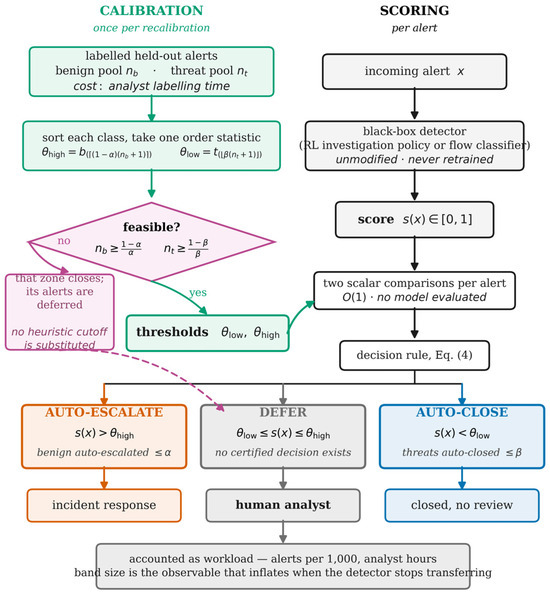
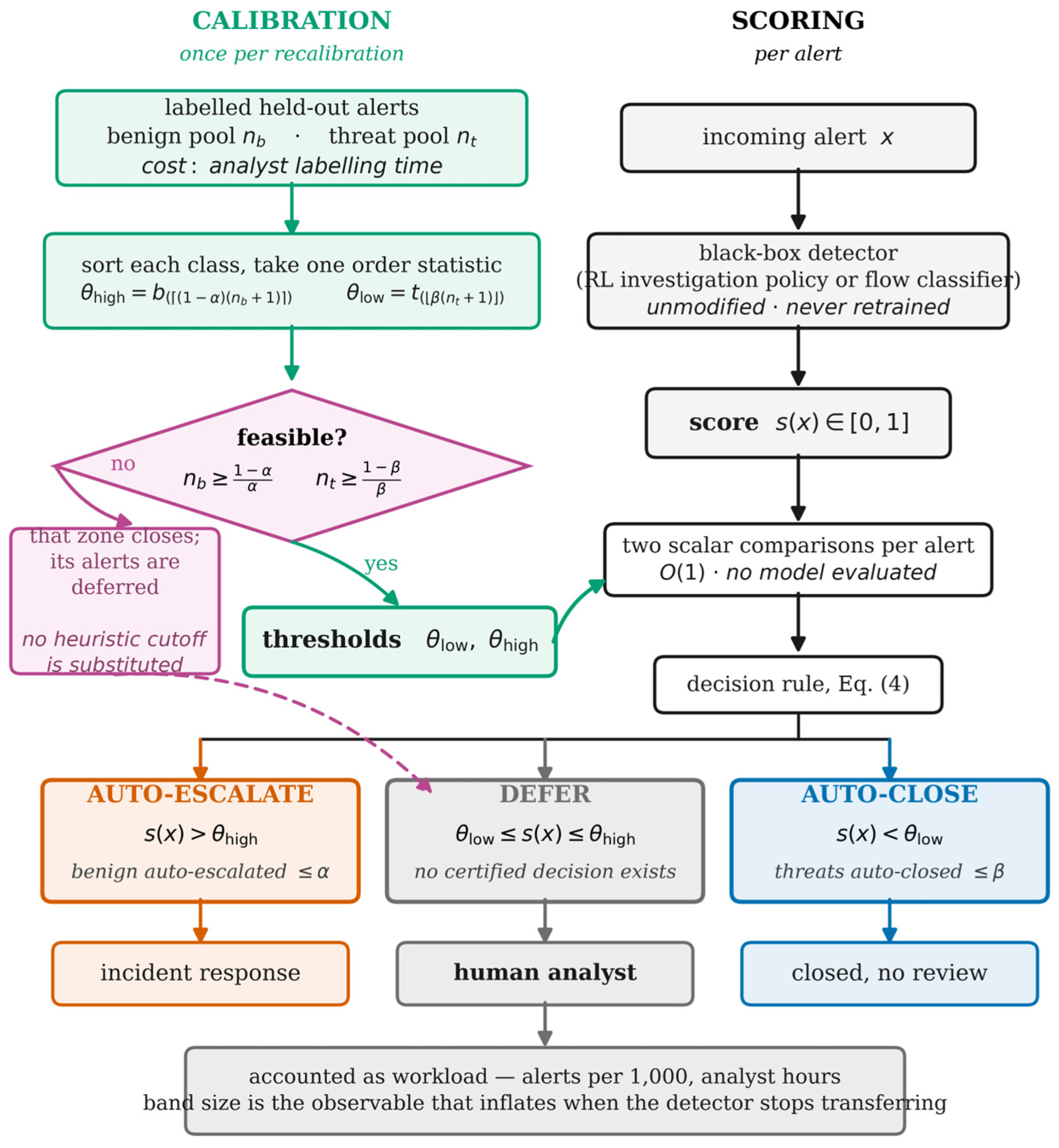
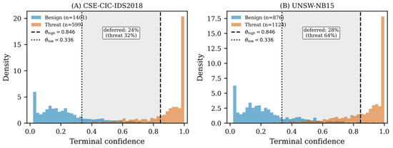
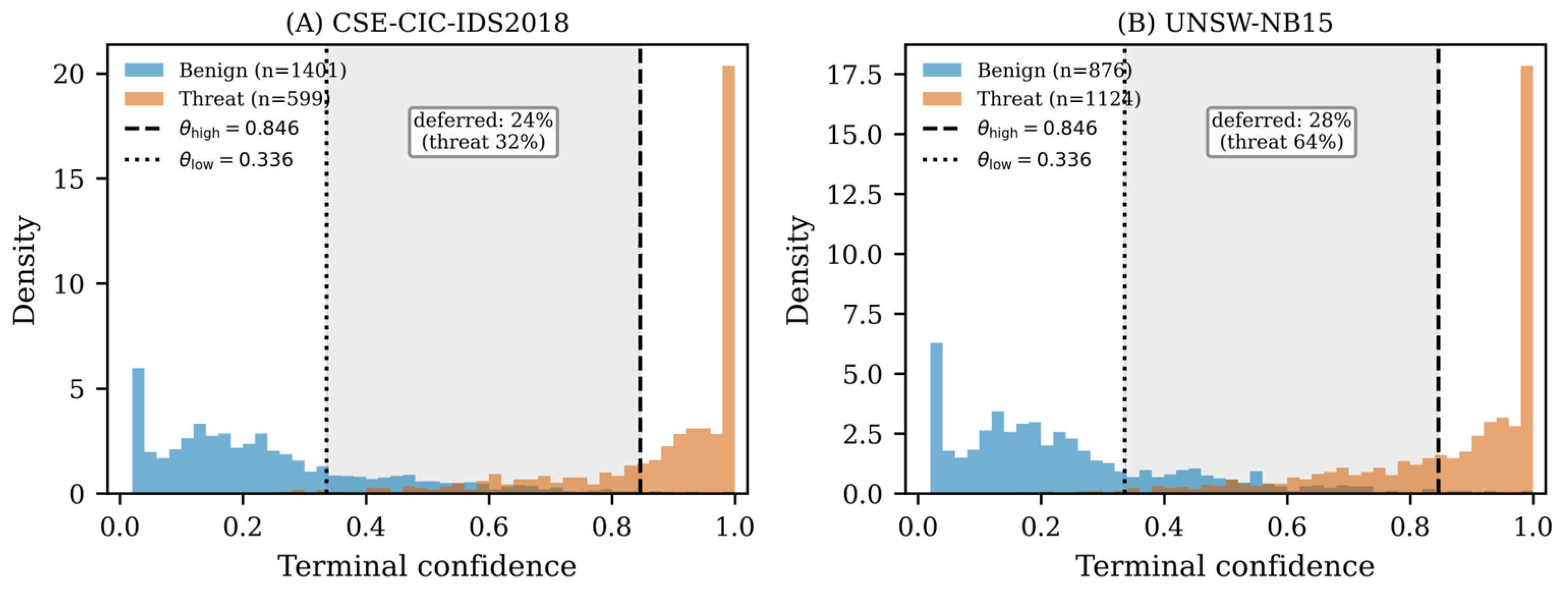
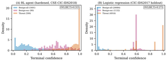
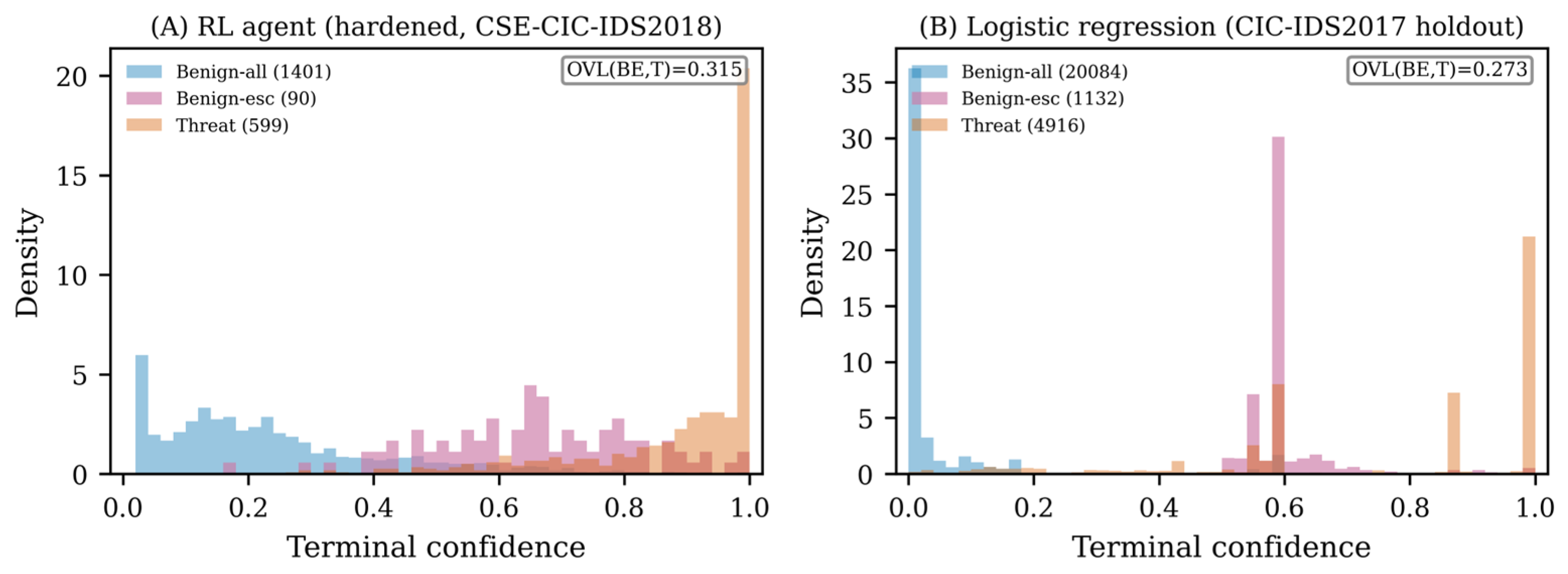
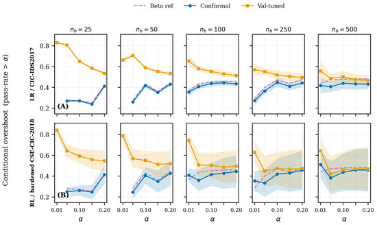
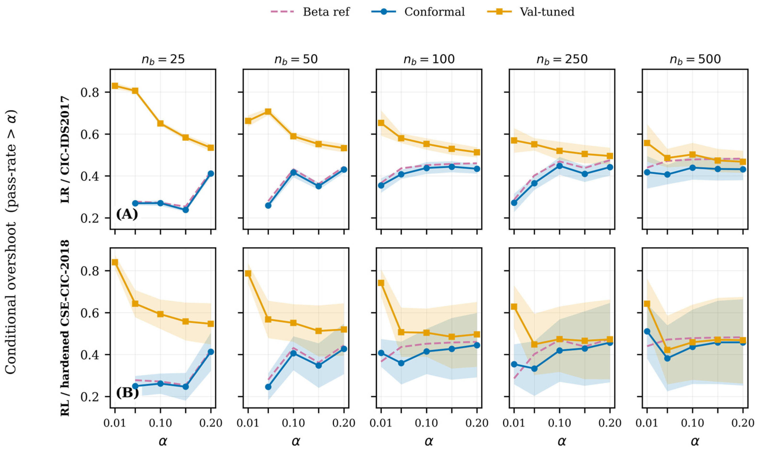
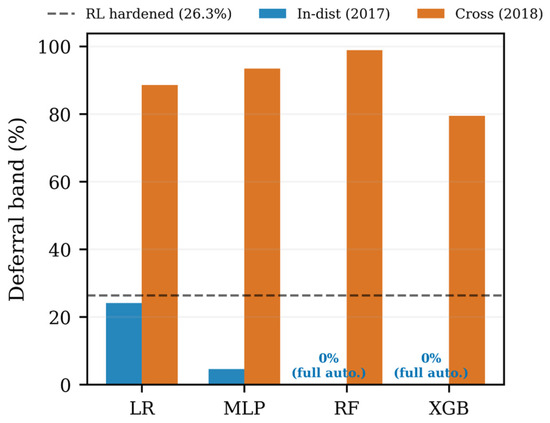
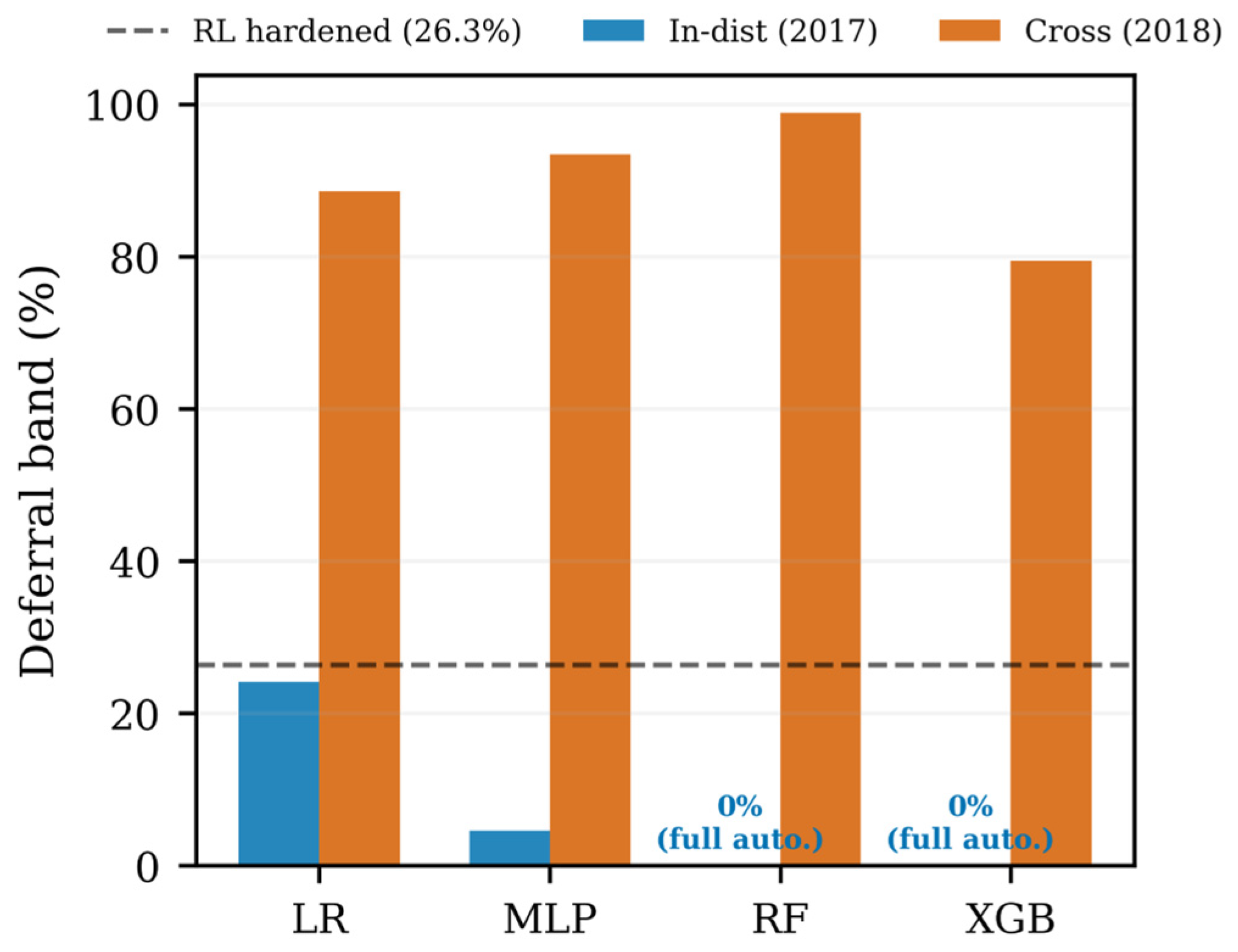
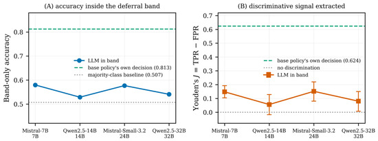
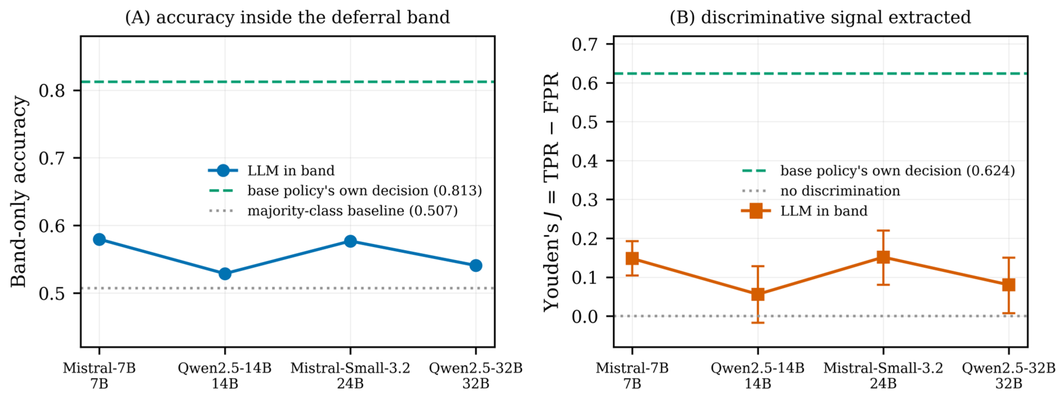
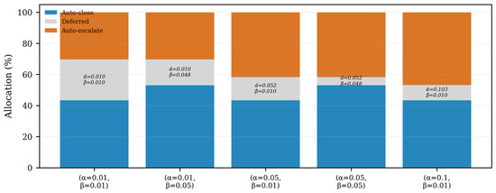
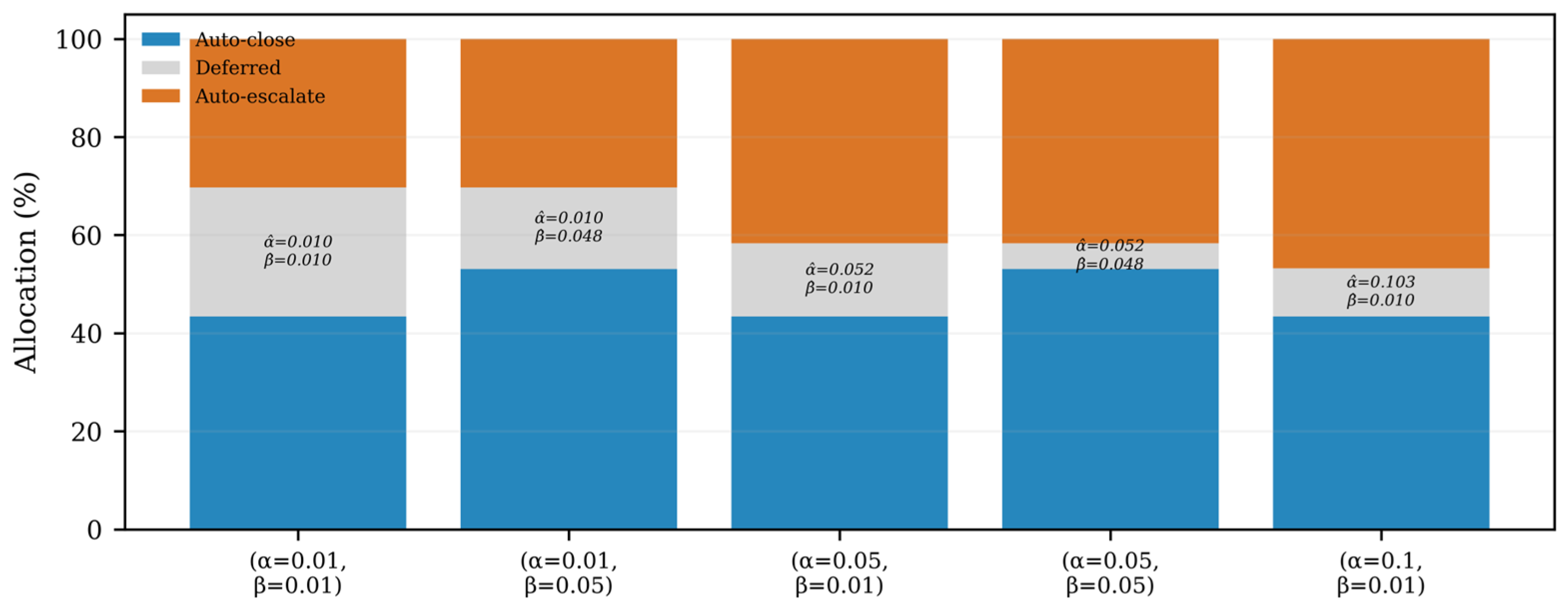

Disclaimer/Publisher’s Note: The statements, opinions and data contained in all publications are solely those of the individual author(s) and contributor(s) and not of MDPI and/or the editor(s). MDPI and/or the editor(s) disclaim responsibility for any injury to people or property resulting from any ideas, methods, instructions or products referred to in the content. |
© 2026 by the authors. Licensee MDPI, Basel, Switzerland. This article is an open access article distributed under the terms and conditions of the Creative Commons Attribution (CC BY) license.