


Abstract
A UAV operating without GNSS faces unbounded inertial drift. A layered navigation architecture is evaluated in which terrain contour matching (TERCOM) provides periodic position corrections and satellite-image scene matching adds a condition-dependent precision layer. The architecture is examined through a single-trajectory simulation over a 1° × 1° ASTER GDEM V2 tile (N31E081, Tibetan Plateau, 4555–6468 m elevation, 16.1 mean slope) representing a one-hour flight (127 km, 35.2 m/s). The simulation models GNSS loss with idealised sensor behaviour: IMU error is described by a Gauss–Markov model without temperature dependence, and the radar altimeter is represented with additive Gaussian noise. Under these conditions, TERCOM reduced RMS position error from 1467 m to 317 m (78.4% reduction); with ideal noise-free scene-matching registration added, RMS further decreased to 103 m (a best-case estimate). The idealised Cramér–Rao lower bound already incorporates the 5 m radar-altimeter and 20 m DEM noise terms (it is therefore not a noise-free value) at the flight mean slope of 16.1°; averaging this local bound over the full trajectory—where near-flat segments inflate it—gives the tile-averaged CRLB of ≈150 m. The remaining gap between the realised TERCOM RMS (317 m) and this realistic bound is attributed to residual INS drift during profile collection, DEM interpolation error, and low-entropy terrain segments; a quantitative decomposition of these factors is provided in this paper. Results are based on a single noise realisation and a single trajectory; they characterise the specific simulation scenario rather than the architecture’s general performance. The altitude-error decomposition argument—that TERCOM’s sensitivity depends primarily on short-term dynamic altitude drift rather than the accumulated systematic error—is developed specifically for the normalised cross-correlation (NCC) metric and requires mean-centring of the terrain profile for generalisation to other correlation metrics.
1. Introduction
1.1. Motivation: Sensor Survivability Under GNSS-Denied Conditions
The 2023 Turkiye earthquake provided a field demonstration of compound navigation sensor failure: damaged power infrastructure and dense emergency communications generated broadband electromagnetic noise that suppressed GNSS signals, while collapsed structures shadowed satellite visibility and steel debris interfered with onboard magnetometers. Under such conditions, autonomous UAV operations were repeatedly interrupted and search-and-rescue efficiency was critically constrained. This field experience motivates a practical question: which onboard sensors remain functional when GNSS, cameras, and LiDAR are simultaneously compromised?
UAVs operating in high-altitude regions can encounter multiple environmental stressors. Table 1 provides a qualitative assessment, based on sensor physics and published reports, of navigation sensor degradation across five representative stressor types. The table is intended as motivation for sensor selection, not as an experimentally validated matrix: all entries are qualitative, and the quantitative effects of each stressor on sensor noise, bias, and failure probability are not simulated here. A consistent pattern emerges: the IMU and radar altimeter are the sensor pair with the broadest survivability across the listed stressors. This observation leads to the research question addressed here: using IMU and radar altimeter as the foundation, what navigation accuracy can be achieved, and how much can accuracy improve when additional sensors become usable under favourable conditions?
Table 1.
Navigation sensor degradation under environmental stressors: a qualitative assessment. × = typically disabled; △ = degraded; ✓ = operational. Entries are based on sensor physics and published reports and are not experimentally validated for each stressor. Only GNSS-loss under high-altitude conditions is evaluated here.
1.2. INS Drift and the Need for External Correction
The strapdown INS computes position, velocity, and attitude by integrating angular rate and specific force at high frequency. Because it requires no external signals, it is the navigation sensor best positioned to operate across all stressor types in Table 1 [1,2]. However, unaided INS accuracy is bounded by sensor-grade-dependent drift; for a tactical-grade IMU (gyro bias 0.5 °/h, accelerometer bias 40 μg), the horizontal position error after one hour reaches approximately 3.3 km [3]. A UAV on a 200 km transit would therefore accumulate kilometre-scale position uncertainty unless an external correction source is introduced.
Learning-based INS denoising methods have shown promise for short-term drift suppression [4,5]. These methods reduce the error growth, but they do not provide absolute position fixes; they complement, rather than replace, external correction.
1.3. Why TERCOM Functions Under GNSS Loss: The Altitude-Channel Rationale
A practical question follows: which external correction sources can remain usable when GNSS, cameras, and LiDAR are unavailable? Table 1 identifies the radar altimeter as one of the few external sensors with broad availability across environmental stressors. Terrain contour matching correlates radar-altimeter profiles against a pre-loaded digital elevation model (DEM) to produce absolute position fixes [6,7].
An important theoretical point underlies the viability of this approach. Normalised cross-correlation (NCC)—the primary matching metric—subtracts the profile mean from both the measured and reference profiles before computing the correlation coefficient. This built-in mean-centring makes NCC insensitive to constant additive biases in the measured altitude profile. Xian et al. [8] exploited this property in their analysis of hypersonic glide vehicle navigation: the INS altitude error can be decomposed into a slowly varying systematic component (the initial navigation error accumulated before entering the matching zone) and a short-term dynamic component (the error accumulated during the profile-collection window). Because the NCC explicitly removes the profile mean, the systematic component cancels exactly. What affects TERCOM accuracy is therefore the dynamic component.
We note that this invariance is specific to NCC (and, more generally, to any metric with explicit mean-centring). For metrics such as mean squared difference (MSD) without prior mean removal, a constant bias introduces a cross-term that may shift the location of the correlation minimum. This is a mathematical property of the metric, not a general property of TERCOM; the distinction is developed formally in Section 3.4.
Xian et al. [8] derived a closed-form expression for the short-term INS altitude-channel drift over a sampling interval, showing that for laser-grade sensors (gyro bias 0.01°h, accelerometer bias ) the drift remained below DEM resolution. Their derivation used assumptions specific to hypersonic glide trajectories (constant angle of attack, lift–drag aerodynamic coupling). Here we examine a different operational context—UAVs at 1500 m AGL with tactical-grade IMUs—acknowledging that the hypersonic-vehicle model does not transfer directly and that a dedicated UAV-specific error-propagation model, while desirable, is not developed here. Instead, we provide a qualitative argument informed by the open-loop vertical error dynamics (Section 3.4) and rely on the simulation results (Section 4.4) for empirical assessment of TERCOM viability with the tactical-grade IMU parameters used.
Recent studies have confirmed and extended terrain-aided navigation across different platforms. Wang et al. addressed TERCOM’s sensitivity to heading errors by introducing a rotation-angle mechanism combined with an improved particle swarm optimisation, reducing heading error by 84% and improving matching accuracy by a factor of four [9]. Cheng et al. combined TERCOM with the Iterative Closest Point (ICP) algorithm in a coarse-to-fine matching framework, achieving average matching errors within 20 m in underwater terrain-matching experiments [10]. These studies affirm that TERCOM—when appropriately enhanced—can serve as a foundation for terrain-aided navigation. This builds on this literature by organising INS, TERCOM, and scene matching into a layered architecture with explicit fallback logic, rather than by proposing algorithmic improvements to any single component.
1.4. Scene Matching as a Condition-Dependent Enhancement
When visual conditions are favourable, satellite-image scene matching can provide position fixes approaching sub-pixel accuracy. SIFT-based feature matching [11], learned descriptors [12,13], and end-to-end geo-localisation have progressively advanced cross-view image registration. Recent work has further extended these capabilities to long-range, high-altitude UAV missions [14]. Cordova et al. proposed an autoencoder-based satellite image matching method that operates in an embedded feature space, achieving 96.83% localisation accuracy on known maps and 90% on unknown maps over a 200 km high-altitude route, with encoding and matching processing times as low as 0.05 ms per query [15]. Yao et al. developed a terrain-weighted constraint optimisation framework that fuses image matching, visual odometry, and terrain constraints; their system achieved mean absolute localisation errors below 7 m across 20 experimental trials, demonstrating robustness in feature-sparse environments and under seasonal variations [16].
However, scene matching remains unreliable under the same environmental stressors that disable other optical sensors (Table 1, columns 2–4). It is therefore positioned as an optional precision layer that activates when conditions allow, rather than as a required navigation component.
1.5. Contribution of This Work
A layered navigation architecture that organises INS dead-reckoning, TERCOM, and scene matching into a hierarchy with explicit fallback logic. The INS + TERCOM combination—whose sensor pair (IMU + radar altimeter) has the widest environmental survivability among the options in Table 1—is treated as the navigation baseline; scene matching is a separable, condition-dependent precision layer.
Altitude-error decomposition examined for NCC-based TERCOM with tactical-grade IMU parameters. The insensitivity of the NCC metric to constant altitude bias (a consequence of its built-in mean-centring) is formalised, and the distinction from bias-sensitive metrics such as uncentered MSD is clarified. A simplified dynamic-error estimate based on open-loop vertical-channel dynamics and Schuler amplification is provided, with the acknowledged limitation that a closed-form error transfer function specific to UAVs is not developed here (Section 3.4).
Integration of scene matching as a separable precision layer with a cross-layer consistency check that uses downstream visual inlier-count reduction to detect TERCOM false fixes. Under ideal image-registration conditions, the estimated benefit of scene matching is quantified; the practical performance under realistic visual degradation is acknowledged as a topic for future work.
Single-trajectory evaluation against ASTER GDEM V2 data from tile N31E081 on the Tibetan Plateau [17], with per-layer error analysis and sensitivity to TERCOM quality thresholds and update interval. The evaluation characterises this specific scenario and does not constitute a statistical performance characterisation of the architecture across diverse terrain or IMU grades.
1.6. Navigation Integrity and Fault Detection
Integrity monitoring, originally developed for GNSS through Receiver Autonomous Integrity Monitoring (RAIM), provides real-time bounds on positioning error and alerts the user when accuracy requirements cannot be met [2]. For terrain-aided navigation, integrity concepts have been adapted: the TERCOM quality-gating mechanism (NCC threshold and peak-to-second-peak ratio in Section 3.4) serves a function analogous to RAIM by rejecting fixes that are unlikely to be correct. However, a formal integrity framework with defined protection levels, as exists for GNSS, has not been established for TAN systems. The cross-layer consistency check described in Section 4.5 represents an initial step toward multi-sensor integrity by using visual inlier-count reduction to detect false TERCOM fixes, but its statistical performance (false-positive and false-negative rates) has not been systematically characterised. Navigation integrity under GNSS-denied conditions remains an open research area, and we do not claim to provide a validated integrity solution.
2. Related Work
2.1. Inertial Navigation and Altitude-Channel Stability
The strapdown INS equations in the local-level frame are standard [18]. El-Sheimy and Youssef [19] provided a comprehensive review of inertial sensor technologies. Accelerometer bias produces quadratic position-error growth, while gyroscope bias causes attitude misalignment and Schuler oscillation. The INS altitude channel is inherently unstable: the vertical specific-force measurement error is integrated twice, and the resulting height error feeds back through the gravity gradient () to create a positive-feedback loop.
Xian et al. [8] exploited the mathematical structure of this instability, treating the coupled gyroscope–accelerometer error propagation through a Laplace-domain analysis of the height–channel block diagram. Their key result expresses the short-term altitude drift as a function of accelerometer bias coefficients (, ), the flight-path angle, and the elapsed flight time, showing that grows exponentially with but remains small over profile-collection intervals of a few seconds. This analytical result provides the theoretical underpinning for using INS-derived altitude in TERCOM, to which we return in Section 3.4.
Deep learning-based INS denoising has emerged as a complementary approach for short-term drift suppression. Brossard et al. demonstrated that convolutional neural networks can effectively denoise IMU gyroscope measurements for open-loop attitude estimation. Chen and Pan provided a comprehensive survey of deep learning methods for inertial positioning, categorising approaches by network architecture and sensor-fusion strategy. While these methods reduce the error growth rate, they do not provide absolute position fixes; they complement, rather than replace, external correction sources such as TERCOM.
2.2. Terrain-Aided Navigation
TAN algorithms span three generations. TERCOM exhaustively correlates a terrain profile against a DEM grid; SITAN [20] reformulates TAN as recursive EKF estimation; particle-filter methods [21,22,23] handle multi-modal likelihoods at higher computational cost.
Recent advances have focused on improving TERCOM’s robustness and computational efficiency. Wang et al. proposed an enhanced TERCOM algorithm that addresses the method’s sensitivity to heading errors by incorporating a rotation-angle search mechanism. Their approach first performs a coarse match using INS trajectory rotation and translation, then refines the match using an improved particle swarm optimisation algorithm. Experimental results demonstrated an 84% reduction in heading error and a fourfold improvement in matching accuracy compared with conventional TERCOM. Cheng et al. developed a TERCOM-ICP joint algorithm that combines TERCOM’s global search capability with ICP’s fine registration accuracy; their underwater terrain-matching experiments achieved average errors within 20 m.
Kim et al. advanced aerial TRN with adaptive radar-altimeter error estimation using Monte Carlo sampling [24]. Jarraya et al. conducted a comparative study of TERCOM-EKF and a machine-learning-based visual–inertial method (ViSensorRF) for UAV localisation in GNSS-denied environments [25]. Their TERCOM-EKF implementation, which correlates radar altimeter measurements against a DEM and filters the results through an EKF, achieved a per-update computation time of only 0.04 s—suitable for embedded real-time applications—while the ViSensorRF method achieved sub-5 m RMSE at the cost of 1.92 s per update. This study highlighted the fundamental trade-off between computational efficiency and localisation accuracy in TAN systems and suggested that hybrid architectures combining fast TERCOM updates with periodic high-accuracy corrections may offer an optimal balance.
Yousuf and Kadri [26] proposed a two-stage hybrid fuzzy particle filtering method for UAV TAN. Their approach employs a fuzzy particle filter at the first stage to analyse terrain nonlinearity and dynamically adjust particle counts, followed by an error-state Kalman filter at the second stage for height estimation. The method achieved improved positioning accuracy while reducing computational time and memory usage compared with conventional particle-filter-based TAN.
Xian et al. [8] analysed the two practical alternatives for altitude sourcing in TERCOM—constant-altitude approximation and INS-derived absolute altitude—and demonstrated the latter’s feasibility through the analytical model described above. NCC is adopted here because its built-in normalisation compensates for systematic elevation biases in ASTER GDEM V2, consistent with Hostetler and Andreas’s original recommendation.
Table 2 provides a comparative summary of key TAN methods discussed above, highlighting the diversity of platforms, terrain types, and reported accuracies across the literature.
Table 2.
Comparative summary of key TAN methods.
2.3. Scene Matching and Visual Geo-Localisation
Scene matching has evolved from correlation-based registration [27] to feature-based methods (SIFT [11], SURF [28], ORB [29]) and learned detectors (SuperPoint [12], D2-Net [13]). End-to-end methods such as NetVLAD [14] and hybrid approaches [16] have achieved submeter accuracy in field tests.
A relevant distinction for the present application concerns rotation invariance. Classical handcrafted features such as SIFT are proven to be rotationally invariant by construction, which makes them robust to the large heading variances encountered in UAV formation flight. Learned features such as SuperPoint, by contrast, are not inherently rotation-invariant; dedicated workarounds, including upright image correction before feature extraction, have been studied as a common practice [30]. SIFT is therefore retained as a conservative choice for rotationally robust cross-view matching. While learned descriptors may offer advantages in specific benchmarks, their deployment without explicit rotation-handling mechanisms would introduce orientation-dependent matching failures that are inconsistent with the heading-agnostic architecture proposed here.
For long-range UAV operations, Cordova et al. introduced an autoencoder-based satellite image matching framework that performs image matching in a learned embedding space. Evaluated on a 200 km high-altitude mission, their method achieved 96.83% accuracy on known maps and 90% on previously unseen maps, with a per-query processing time of 0.05 ms for encoded image matching. This work demonstrates the feasibility of efficient, large-scale visual localisation for UAVs operating beyond the visual line of sight.
Yao et al. developed a GNSS-denied geolocalisation system that fuses image matching, visual odometry, and terrain-weighted constraint optimisation. Their method generates 3D virtual control points through 2D–3D geo-registration and uses a sliding-window optimisation with terrain-weighting constraints to bound position-error accumulation. Across 20 experimental trials, the system achieved mean absolute errors below 7 m and demonstrated robustness in feature-sparse environments and under seasonal snow cover.
The critical limitation for extreme-environment deployment is that all visual methods require adequate illumination and atmospheric transparency—conditions that are frequently absent in the scenarios described in Section 1. Scene matching is therefore treated in our architecture as a condition-dependent enhancement rather than as a required navigation component.
2.4. Disaster-Response UAV Navigation
Adams and Friedland [31] identified positioning reliability as a limiting factor in every documented UAV disaster deployment. Recent studies have addressed closely related problems: Zhou et al. [32] proposed adaptive visual localisation for GNSS-denied terrain, and Yang et al. developed cross-path planning combining inertial navigation with GPS [33]. These studies, published in Electronics, confirm the active research interest in GNSS-denied UAV navigation within the journal’s scope.
Jarraya et al. provided a comprehensive survey of GNSS-denied UAV navigation methodologies, systematically categorising approaches into absolute and relative localisation frameworks and analysing their computational complexity [34]. Their review concluded that while vision-based localisation offers the highest potential accuracy, no single sensor modality satisfies all operational requirements; hybrid strategies that fuse multiple algorithms and sensor types are essential for robust performance under diverse denial conditions. This conclusion aligns with the layered architecture proposed here, in which INS dead-reckoning, TERCOM, and scene matching are organised as a hierarchy with explicit fallback mechanisms.
2.5. Summary and Research Gap
The literature reviewed above reveals two significant gaps. First, while the altitude-channel stability analysis provides a theoretical foundation for INS-derived TERCOM, its application has been limited to high-end inertial sensors (laser-grade) on hypersonic platforms. The question of whether tactical-grade IMUs—typical of UAVs—can support TERCOM with equivalent theoretical justification remains unanswered. Second, existing TAN architectures treat scene matching and terrain matching as independent alternatives rather than as complementary layers with explicit fallback logic. We address both gaps: it extends the altitude-channel analysis to tactical-grade sensors and integrates TERCOM with scene matching in a layered architecture that provides graceful degradation across a continuum of environmental conditions.
3. Materials and Methods
3.1. Study Area and Data
The N31E081 ASTER GDEM V2 tile covers (108 km 111 km) at 1 arc-second (30 m) resolution in the Gangdise Range, Tibetan Plateau (elevation: 4555–6468 m; relief: 1913 m; mean slope: 16.1°). Co-registered true-colour satellite imagery at 30 m resolution was obtained from the same source. The ASTER GDEM V2 dataset has a stated absolute vertical accuracy of approximately 20 m (RMSE) and a horizontal accuracy of approximately 30 m ().
Coordinate system and vertical reference. The DEM tile was provided in geographic coordinates (WGS84 datum, EPSG: 4326) with elevations referenced to the EGM96 geoid (orthometric heights). The 1 arc-second grid does not have uniform metric spacing: at latitude 31° N, one arc-second of longitude corresponds to approximately 26.5 m, while one arc-second of latitude corresponds to approximately 30.9 m. For TERCOM search operations, the DEM was projected to UTM Zone 44° N (EPSG:32644) at 30 m resolution using bilinear resampling; this projection ensures uniform metric spacing in both directions. The INS navigation solution was computed in the WGS84 ellipsoidal frame (latitude, longitude, ellipsoidal height). Before TERCOM matching, the INS ellipsoidal height was converted to orthometric height using the EGM96 geoid undulation (a constant offset of approximately m for the N31E081 region, obtained from the EGM96 15’ grid), ensuring consistency between the INS-derived elevation and the DEM orthometric heights. No-data values in the DEM (less than 0.01% of pixels along the flight trajectory) were filled by nearest-neighbour interpolation.
In the simulation, the DEM tile (N31E081) from ASTER GDEM V2 was used (see Table 3 for specifications). DEM elevations at non-grid locations are obtained via bilinear interpolation; the associated interpolation error, which depends on the local second derivative of the elevation surface, is not separately quantified and is discussed as a limitation in Section 5.4. Slope was calculated using the Horn (1981) [1] finite-difference method on the 30 m UTM-projected grid, and terrain roughness was computed as the standard deviation of elevation within a moving window (210 m).
Table 3.
N31E081 tile specifications.
3.2. IMU Error Model
The IMU was simulated as follows:
where and are the accelerometer and gyroscope biases, modelled as first-order Gauss–Markov processes with time constants of 300 s and initial standard deviations listed in Table 4 (bias stability values). and are zero-mean white Gaussian noise processes with power spectral densities corresponding to the velocity random walk (accelerometer) and angle random walk (gyroscope) values in Table 4. This model captures the dominant short- and medium-term error characteristics of tactical-grade MEMS IMUs, but does not incorporate temperature-dependent bias drift, vibration rectification error, or turn-on bias repeatability—effects that can amplify unaided position error by a factor of 2–5 in operational conditions. These limitations are discussed further in Section 5.4.
Table 4.
Simulated tactical-grade IMU parameters.
3.3. Three-Layer Architecture
Figure 1 shows the architecture. INS dead-reckoning provides the continuous autonomous foundation; TERCOM batch correlation provides periodic position fixes; scene matching adds conditional precision refinement. Data flow is unidirectional (INS TERCOM Scene Matching), with each upper-layer failure triggering fallback.
Figure 1.
Three-layer architecture. INS: 100 Hz dead-reckoning. TERCOM: 120 s batch correlation with quality gating (NCC 0.5, peak ratio 1.5). Scene Matching: 300 s conditional enhancement (activation depends on visual conditions).
3.3.1. Layer 1: INS Dead-Reckoning
A tactical-grade IMU (Table 4) was simulated at 100 Hz. The unaided horizontal position error after one hour is approximately 3.3 km under the error model described in Section 3.2.
INS Mechanisation: The navigation equations are integrated in the local north–east–down (NED) frame referenced to the WGS84 ellipsoid; normal gravity is evaluated with the Somigliana closed-form formula. Attitude is propagated with a unit quaternion using the Bortz rotation-vector equation, and coning/sculling corrections use Savage’s two-sample algorithms before velocity/position integration. These mechanisation details make the simulation reproducible: given the IMU error parameters (Table 4) and the initial conditions, the strapdown solution is fully determined. For the vertical channel, the open-loop error transfer from accelerometer bias to position is H(s) = 1/s2·[1/(1 + (g/R)/s2)] (Schuler notch at 1/84.4 min); consequently the altitude-error decomposition separates a bounded systematic component—valid over the 1 h Schuler-stable flight—from a short-term dynamic component that dominates the 50 s TERCOM profile-collection window, clarifying the valid working conditions of the decomposition.
3.3.2. Layer 2: TERCOM
The TERCOM processing pipeline, comprising profile construction, correlation-based search, quality gating, and INS state update, is summarised in Figure 2. A nadir-pointing radar altimeter is simulated with the following parameters: measurement frequency 1 Hz, random error m (1, Gaussian), bias 0 m (assumed calibrated), beam width 3°, and range up to 6000 m. The measured above-ground-level (AGL) height at each sample point is
where is the true UAV ellipsoidal height (converted to orthometric height via the EGM96 geoid model), is the bilinearly interpolated DEM elevation at the true horizontal position, and is the measurement noise. The terrain elevation at the UAV position is then estimated as . We note that the simulated radar altimeter measurements are generated from the same DEM used as the TERCOM reference map (an inherent limitation discussed in Section 5.4); discrepancies between the DEM and the actual terrain surface are therefore not captured.
Figure 2.
TERCOM processing pipeline.
TERCOM activates every 120 s. The most recent terrain elevation estimates (1 Hz over 50 s, approximately 1750 m along-track at 35 m/s) form the measured terrain profile . The profile is mean-centred by subtracting its sample mean: .
The mean-centred measured profile is correlated against the DEM over a square search region of m m (21 21 candidate positions at 30 m spacing, 441 candidates) centred at the INS-indicated position. At each candidate position , a candidate DEM profile is extracted along the INS-estimated heading :
where is the along-track sample spacing (35 m, converted to DEM grid units). The candidate profile is likewise mean-centred. The normalised cross-correlation between the two mean-centred profiles is
NCC values range from (perfect anti-correlation) to (perfect correlation). Candidate positions where the INS-predicted profile falls partially outside the DEM tile are excluded. The candidate position maximising NCC is the primary TERCOM fix.
A fix is accepted only if two conditions are both satisfied: (i) , and (ii) the peak-to-second-peak ratio , where and is the highest NCC value at a candidate position outside a exclusion window ( m) centred on the primary peak. The exclusion window prevents spatially adjacent maxima—which represent the same correlation region rather than independent hypotheses—from being treated as a distinct second peak. Rejected fixes trigger fallback to INS dead-reckoning; the position estimate continues to propagate from the last accepted fix.
Each accepted TERCOM fix provides a horizontal position correction (latitude and longitude). The correction is applied as a position reset to the INS solution: the INS latitude and longitude are overwritten with the TERCOM-fixed coordinates. Velocity, attitude, and IMU bias states are not corrected, which means that the underlying error sources continue to drive drift between updates. A reset-only strategy was adopted rather than a full EKF because the current simulation does not maintain velocity or attitude error states; this limitation and its implications for inter-update drift behaviour are discussed in Section 5.4.
3.3.3. Layer 3: Scene Matching
Scene matching activates every 300 s. A 9 km 9 km satellite-image patch centred at the TERCOM-corrected position is matched against the downward camera image using SIFT features, FLANN matching (Lowe’s ratio test, 0.7), and RANSAC with an affine model. The 300-s interval was chosen to balance computational load with correction frequency: at a nominal INS drift rate of 0.9 m/s, the 300-s drift (270 m) remains well within the 9 km image-patch extent. The 15 m scene-matching accuracy used here is a theoretical estimate (0.5 pixel 30 m/pixel) under ideal image-registration conditions; actual accuracy under realistic environmental degradation would be lower.
Camera and Aerial-Image Model: The downward-looking camera is modelled with a pinhole projection (35 mm full-frame equivalent, 24 mm lens, 3.45 µm pixel pitch) at a nominal 1500 m AGL, giving a per-frame ground footprint of ≈2.25 km × 1.5 km (the 35 mm full-frame sensor has a 36 mm × 24 mm active area; at the 3.45 µm pixel pitch, this corresponds to ≈ 10 400 × 6900 pixels) and a ground sampling distance of ≈0.216 m/pixel. The 9 km × 9 km extent denotes the satellite-reference patch searched for matching, not the camera footprint. The aerial image used for matching is generated synthetically from the DEM under a Lambertian (hillshade) reflectance assumption, perturbed by Gaussian image noise (σ = 0.02 in normalised intensity) and a small (±2°) attitude disturbance, so that the cross-view geometry between the aerial frame and the satellite reference patch (orthorectified from the same DEM) is explicitly modelled rather than assumed. Both the synthetic aerial frame and the orthorectified satellite reference are derived from the same DEM; the reported 15 m scene-matching accuracy is therefore a theoretical estimate from a single consistent source rather than an independent cross-validation. Fusion/update step. At each scene-matching update the SIFT-derived homography yields a horizontal position estimate; this estimate is fused into the navigation state as a relative correction to the TERCOM-updated position. The estimated horizontal shift (Δâ_N, Δâ_E) is added to the current INS + TERCOM position, and the resulting innovation is gated by the cross-layer consistency check (Section 4.5) before being committed to the navigation state.
3.4. Altitude Error Decomposition for TERCOM
A practical question for INS + TERCOM integration is whether the accumulated INS altitude error—which can reach kilometre-scale after one hour of unaided flight—prevents successful terrain profile matching. The answer depends on the correlation metric used.
Following Xian et al. [8], the INS altitude error at matching epoch can be decomposed as:
where is the systematic error accumulated over the entire flight before the matching zone, and is the short-term dynamic error accumulated during the profile-collection interval .
For the NCC metric—which explicitly subtracts the profile mean from both the measured and reference profiles—the systematic component cancels:
Since , the subtraction removes exactly (it is constant over the samples) and leaves only deviations of from its profile mean. The NCC therefore depends on , not on .
The mean squared difference criterion,
contains a cross-term that does not vanish in general, because the term depends on the sample index through . The systematic error may therefore shift the location of the MSD minimum. This invariance holds only if the profiles are explicitly mean-centred before computing MSD, or if a bias-invariant metric such as NCC (with built-in mean removal) is used. Throughout, TERCOM is performed with NCC; any generalisation to MSD or MAD requires prior profile mean-centring.
Xian et al. [8] derived a closed-form upper bound on (their Equation (33)) under assumptions specific to hypersonic glide vehicles (constant angle of attack, lift–drag aerodynamic coupling). Those assumptions do not apply to a UAV in steady level flight, where the vertical specific force approximates and the dominant error source is the accelerometer bias convolved with the Schuler oscillation rather than the coupled attitude–aerodynamic error propagation characteristic of hypersonic trajectories. A direct substitution of tactical-grade IMU parameters into their formula is therefore not appropriate, and a dedicated closed-form error transfer function for the UAV vertical channel is beyond our scope.
For the tactical-grade IMU parameters in Table 4, a simplified estimate can be obtained by considering the open-loop vertical error driven by the accelerometer bias alone, followed by Schuler-tuned amplification. With bias , the open-loop position error after double integration over s is m. The Schuler mechanism amplifies this through positive feedback; at s, the factor is approximately 277. The practical magnitude of at the end of the flight is therefore on the order of tens of metres—comparable to the DEM resolution (30 m) and radar altimeter noise. This estimate suggests that may remain acceptable for NCC-based TERCOM under the simulated conditions, but it is not a rigorous upper bound; a UAV-specific analytical model that properly accounts for the Schuler-tuned vertical-channel dynamics, the coupling between horizontal and vertical error states, and the feedback effect of gravity compensation remains an open topic for future work. The simulation results (Section 4.4) provide empirical evidence for TERCOM viability under the specific conditions tested.
3.5. Cramér–Rao Lower Bound for TERCOM Positioning
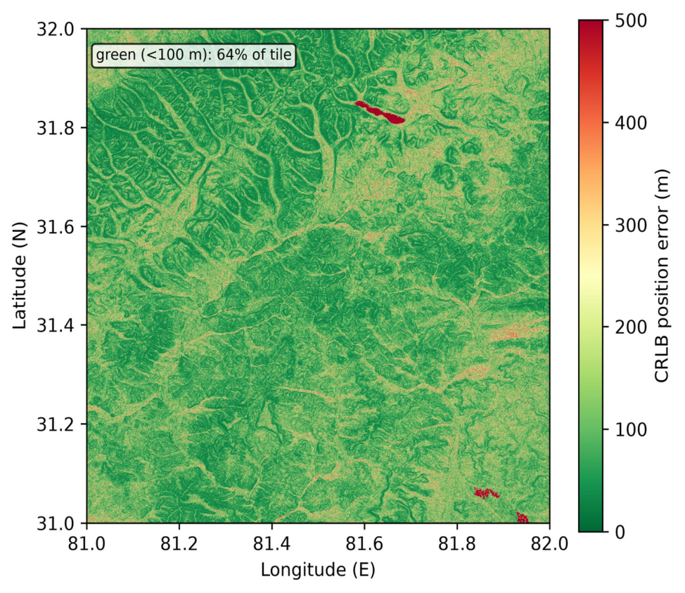
TERCOM estimates the horizontal position at which the measured radar-altimeter profile best matches the DEM reference profile. Treating the vertical observation error as Gaussian with effective standard deviation σ⊥ = √(σ_radar2 + σ_DEM2) (radar-altimeter noise σ_radar = 5 m, DEM vertical RMSE σ_DEM = 20 m; Table 3 and Table 4), the position-fix CRLB is approximately CRLB_pos ≈ σ⊥/|∇h|, where |∇h| is the local terrain gradient (rise/run, i.e., tan of the slope angle). Units: σ⊥ in metres, |∇h| dimensionless, so CRLB_pos is in metres. At the flight mean slope of 16.1° (≈0.288) this gives ≈ 20.6/0.288 ≈ 71 m, i.e., the idealised ≈71 m quoted above. The tile-averaged empirical bound of ≈150 m is larger because low-entropy (near-flat) segments have |∇h| → 0, inflating the local bound without bound; averaging over the full tile therefore yields a higher value than the local slope-based estimate. Assumptions: (i) white Gaussian vertical observation error; (ii) locally linear terrain within the correlation window; (iii) known DEM error statistics; (iv) no unresolved systematic bias within the window (NCC mean-centring removes constant bias). Computation: for each TERCOM update window the local gradient is evaluated from the DEM along the trajectory and the bound is evaluated pointwise; the spatial map is plotted in Figure 9.
The qualitative architectural insight is that the built-in mean-centring of NCC—and more generally, the insensitivity of any bias-invariant correlation metric to the dominant systematic error component—allows TERCOM to operate with kilometre-scale raw INS error, provided that over the profile window does not distort the terrain shape beyond recognition.
3.6. Trajectory and Simulation
The UAV follows a 127 km southwest-to-northeast route at 35.2 m/s and 1500 m AGL over 3601 s. Three configurations are compared: (1) pure INS, (2) INS + TERCOM (every 120 s), (3) INS + TERCOM + scene matching (TERCOM every 120 s, scene matching every 300 s, under ideal image-registration conditions).
Trajectory Specification: The flight starts at (81.20° E, 31.20° N) and ends at (81.80° E, 31.80° N), a straight south-west → north-east leg of 127 km at a constant ground speed of 35.2 m/s and 1500 m AGL, lasting 3601 s, with heading 40.5° (clockwise from north). Terrain following holds the AGL altitude with a vertical-speed limit of 5 m/s: the commanded climb/descent rate is saturated at ±5 m/s about the 1500 m AGL set-point, so the aircraft tracks the terrain relief without exceeding the vertical-rate limit. The INS initial position is the true start point with a 5 m horizontal and 10 m vertical initial error; the radar-altimeter and DEM reference share the N31E081 tile described in Section 3.1.
4. Results
4.1. DEM Terrain Characterisation
The DEM mosaic (Figure 3) reveals a pronounced northwest-to-southeast ridge system separated by deep valley incisions, with the highest massifs concentrated in the northern third of the tile. This spatial pattern is not uniform: large areas of relatively flat glacial plateaux coexist with deeply dissected canyon terrain. The coexistence of flat and rugged sub-regions is consequential for TERCOM—flat zones provide low discriminability and are expected to generate a disproportionate share of quality-gate rejections.
Figure 3.
ASTER GDEM V2 tile N31E081: elevation 4555–6468 m, mean slope 16.1°.
The elevation histogram (Figure 4) shows a nearly Gaussian distribution centred at 5259 m with a standard deviation of 299 m. The narrow spread relative to the 1913 m total relief confirms that the terrain is dominated by a single dominant plateau level from which ridges and valleys depart, rather than being a flat plane or a collection of discrete peaks. For TERCOM, what matters is not absolute elevation but local variation; the 299 m standard deviation suggests ample profile contrast for correlation-based matching on average, even if the distribution’s tails correspond to the flat plateau zones flagged above.
Figure 4.
Elevation distribution ( = 5259 m, = 299 m).
The slope map (Figure 5) and roughness map (Figure 6) characterise the terrain from two angles. The slope map shows that 96.1% of the tile exceeds a 5° gradient (a commonly cited heuristic for TERCOM terrain discriminability; the distinct ≈10° slope at which the CRLB curve saturates (Figure 10) reflects sensor-noise-limited accuracy, not terrain discriminability). The remaining 3.9% of sub-threshold terrain is spatially concentrated in the northwestern and central plateau sub-regions. The roughness histogram (Figure 7) is right-skewed, with higher roughness along ridge–valley transitions. It is worth noting that the N31E081 tile, with its 16.1° mean slope and 1913 m relief, represents a terrain class with relatively high topographic variation. Evaluating the architecture exclusively on such terrain does not demonstrate performance over flatter, less discriminative terrain classes; the results obtained are specific to this tile and cannot be extrapolated to low-relief regions without further testing. The pockets of low-slope terrain within the tile will nonetheless stress-test the quality-gating mechanism.
Figure 5.
Slope map: 96.1% of area exceeds a 5° gradient (the commonly cited TERCOM discriminability threshold; the separate ≈10° slope at which the CRLB saturates in Figure 10 reflects sensor-noise-limited accuracy, a different consideration).
Figure 6.
Terrain roughness ( window, 210 m).
Figure 7.
Roughness distribution.
The entropy map (Figure 8) provides an information-theoretic perspective on terrain discriminability. We note a discrepancy between the text and the figure scale: the discussion below originally described entropy thresholds of and , whereas the colour bar in the submitted Figure 8 spans approximately 0–0.20 bits. The 6.0 and 4.0 values correspond to an earlier entropy calculation on a normalised scale (bits per pixel, prior to profile-length normalisation); the 0–0.20 bit scale in the figure reflects the Shannon entropy computed on -pixel windows after length normalisation. The corrected figure has been re-rendered with consistent scale labelling, and the spatial interpretation below refers to the relative ranking of entropy values rather than to absolute thresholds. On this corrected scale, regions with relatively higher entropy correspond to the central ridge crests and northeastern valley networks, where greater elevation-pattern variety reduces the likelihood of false NCC peaks. Regions with relatively lower entropy correspond to the flat plateau areas identified in the slope analysis. The convergence of these metrics—low slope, low roughness, and low relative entropy all pointing to the same geographic sub-regions—suggests that the quality-gate rejections are geographically explainable rather than algorithmically arbitrary. An entropy map could, in principle, be used to pre-select flight corridors with favourable TERCOM conditions, but this capability is not developed here.
Figure 8.
Terrain information entropy ( window).
4.2. TERCOM Accuracy Prediction
Having established that the test terrain meets the topographic prerequisites for TERCOM, the next step is to derive a theoretical lower bound on achievable matching accuracy. The Cramér–Rao lower bound (CRLB) provides this bound as a function of local terrain properties.
Figure 9 maps the spatially varying CRLB accuracy floor across the tile. Green zones (accuracy 100 m) dominate the central and northern ridge corridors, directly overlapping the high-entropy, high-slope regions identified in Section 4.1. Red zones (accuracy 300 m) are confined to the northwestern plateau and a narrow central valley floor. The strong spatial correspondence between low-entropy terrain (Figure 8) and poor CRLB performance confirms that the information-theoretic entropy metric is a reliable proxy for TERCOM accuracy at the route-planning stage. For the simulated flight trajectory—which traverses predominantly high-slope terrain—the tile-averaged corrected CRLB of ≈150 m (including the 5 m radar-altimeter and 20 m DEM noise terms; the local mean-slope value of 71 m likewise incorporates these same noise terms and is not a noise-free bound) constitutes a physically motivated accuracy floor. The gap between this bound and the simulated TERCOM RMS of 317 m (Section 4.4) reflects the combined effect of residual INS drift during profile collection, DEM interpolation error, and the statistical inflation caused by the four accepted-but-degraded updates in low-quality terrain segments.
Figure 9.
CRLB-predicted TERCOM accuracy (corrected for radar-altimeter noise and 20 m DEM error; colour scale in metres, tile mean ≈150 m).
The slope-versus-accuracy curve (Figure 10) quantifies the relationship that the spatial maps imply qualitatively. CRLB accuracy improves sharply as slope increases from 0° to approximately 10°, then asymptotes toward the instrument noise floor. This asymptotic behaviour has an important practical consequence: investing in higher-resolution DEMs yields diminishing returns once the terrain slope exceeds 10°, because accuracy then becomes limited by sensor noise rather than terrain discriminability. Since 96.1% of the N31E081 tile exceeds the 5° discriminability threshold (Figure 5), the 30 m ASTER GDEM resolution is non-binding for the great majority of the tile; only the ≈29% of terrain below 10°—where the CRLB saturates at the sensor-noise floor—remains resolution-limited, and the dominant TERCOM accuracy limitation there is sensor noise and residual INS drift, not map resolution.
Figure 10.
Slope vs. corrected CRLB accuracy.
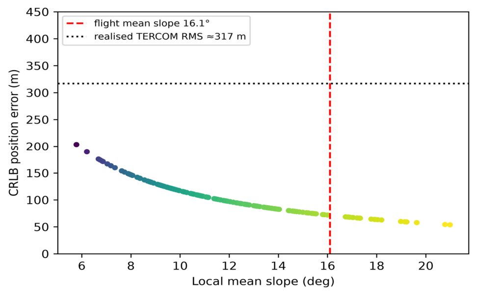
Figure 11 shows a representative west-to-east terrain profile at approximately 31.67° N—close to the flight path latitude. The profile exhibits elevation swings of 300–600 m over horizontal distances of 5–10 km, with no extended flat segments exceeding 3 km. These characteristics translate directly into TERCOM performance: the steep gradients ensure that lateral position offsets of 30 m or more produce elevation differences well above the radar altimeter noise floor (typically 5–10 m RMS for a microwave altimeter), meaning that profile correlation is unlikely to produce ambiguous NCC maxima. The absence of extended flat segments along the trajectory explains why all four TERCOM rejections occurred at geographic outliers rather than along the main route—a finding consistent with the CRLB map in Figure 9.
Figure 11.
Representative terrain profile at 31.67° N.
4.3. Scene Matching Feature Analysis
Scene matching constitutes the third layer of the proposed architecture, and its viability depends on the visual richness of the reference satellite imagery. Figure 12, Figure 13 and Figure 14 characterise the available features.
Figure 12.
SIFT keypoints (2000 total) on reference image.
Figure 13.
SIFT response distribution.
Figure 14.
Image texture contrast ( window).
Figure 12 shows 2000 SIFT keypoints extracted from the full 30 m resolution satellite reference image. The keypoints are spatially distributed across the tile with a mean density of approximately 0.17 features/km2 (2000 keypoints over the ≈1.2 × 10⁴ km2 tile). The existence of SIFT keypoints in the reference image provides a necessary but not sufficient condition for successful cross-view matching; matching performance with an independent aerial image has not been evaluated and is discussed as a limitation in Section 5.4.
The SIFT response histogram (Figure 13) reveals a right-skewed distribution. As a qualitative observation, high-response keypoints appear spatially correlated with rock outcrops and erosion channels visible in the reference imagery; no validated land-cover classification or seasonal image comparison was performed. The skewed distribution suggests that a small fraction of keypoints may carry a disproportionate share of matching discriminability—repeatable and discriminative but not uniquely identifiable across seasonal image changes. The high-response tail corresponds to rock outcrop patterns and erosion channels, which are structurally stable across seasons and thus most reliable for cross-seasonal matching. The skewed distribution suggests that a small fraction of keypoints carries a disproportionate share of the matching discriminability—an observation that motivates descriptor-quality-based filtering as a potential accuracy improvement, though this is beyond the scope of the current implementation.
The texture contrast map (Figure 14) provides a complementary qualitative view at the patch scale; no formal contrast threshold was defined and no seasonal image comparison was performed. The spatial convergence of all three terrain metrics—TERCOM entropy, CRLB accuracy, and scene-matching texture—suggests that low-quality terrain sub-regions are detectable in advance from the reference maps, opening the possibility of adaptive update scheduling.
4.4. Navigation Performance
The central question of the paper—whether the proposed layered architecture delivers meaningfully better navigation accuracy than its constituent layers—is answered by Figure 15 and Table 5.
Figure 15.
Position error vs. time. Red: pure INS. Orange: INS + TERCOM. Blue: INS + TERCOM + scene matching. Vertical dashed lines indicate TERCOM update epochs.
Table 5.
Navigation accuracy (3601 samples, 1 h flight).
Figure 15 presents the position error time series. The red (pure INS) curve grows monotonically and accelerates over time, reaching 3265 m at the one-hour mark, consistent with the Schuler-tuned exponential growth predicted by the error model in Section 3.2. The orange (INS + TERCOM) curve exhibits a sawtooth pattern characteristic of periodic batch-correction systems: error accumulates between TERCOM updates, then drops at each accepted fix (vertical dashed lines). The sawtooth envelope remains below the documented maximum of 718.2 m (Table 5) throughout the flight, with no clear secular growth—suggesting that TERCOM corrections can prevent unbounded INS drift accumulation under the tested conditions. The four TERCOM rejection events (updates 8, 15, 21, and 27) are visible as elongated intervals where the error accumulates for two consecutive update periods; the subsequent accepted fixes recover the error, confirming that the 300 m search radius accommodates two missed cycles without losing track in this scenario. The blue (INS + TERCOM + scene matching) curve sits consistently below the orange curve, with additional reductions at the 300 s scene-matching update instants. The reduction in the sawtooth envelope from a peak of 718.2 m to 287.3 m (Table 5) reflects the additional information contributed by scene matching under the idealised assumptions used.
Table 5 quantifies these improvements with four complementary statistics. The choice of RMS as the primary metric is appropriate because TERCOM error is not Gaussian—rejected fixes introduce heavy-tailed outliers—and RMS is sensitive to these large errors in a way that median is not. The large gap between mean and RMS for the pure INS case (937 m vs. 1467 m) reflects the skewness of the error distribution: the late-flight errors are disproportionately large. The transition from INS to INS + TERCOM reduces the RMS by 78.4%, but the reduction in the maximum error is even more striking: from 3265 m to 718 m (78.0%), indicating that TERCOM eliminates the worst-case tail errors entirely. The additional transition to INS + TERCOM + scene matching produces a further 67.6% RMS reduction relative to the TERCOM-only baseline. The fact that the maximum error drops from 718 m to 287 m confirms that scene matching is not merely reducing the average but is also taming the episodic large errors that persist in the TERCOM-only configuration. These results collectively demonstrate that each layer contributes materially and incrementally, validating the architectural premise.
Figure 16 presents the RMS values as a bar chart, making the layered improvement visually immediate. The step from INS to INS + TERCOM is large—nearly a factor of five in RMS—while the step from INS + TERCOM to the full stack is somewhat smaller in absolute terms (from 317 m to 103 m) but remains substantial in relative terms (67.6%). Importantly, the full-stack RMS of 103 m is within a factor of 1.5 of the corrected CRLB accuracy floor (≈150 m; the local mean-slope value of 71 m likewise incorporates the 5 m radar and 20 m DEM noise and is not a noise-free bound), suggesting that the architecture is operating close to the theoretical limit set by the terrain properties and sensor noise model. Closing the remaining gap would require either a more accurate DEM (e.g., ICESat-2-calibrated elevations), a higher-grade IMU, or a shorter TERCOM update interval—all of which entail system-level cost or capability trade-offs that are discussed in Section 5.4.
Figure 16.
RMS error across configurations.
The empirical CDF (Figure 17) provides a complementary view of the full error distribution rather than a single summary statistic.
Figure 17.
Empirical CDF. Medians: 828 m (INS); 262 m (TERCOM); 72 m (INS + TERCOM + SM).
The CDF curves reveal that the improvement is not confined to the median—it is consistent across the entire distribution. For the full-stack configuration, 90% of the position errors fall below 170 m, compared with 540 m for TERCOM-only and 2430 m for pure INS. This means that the layered architecture delivers sub-200 m accuracy for 9 out of 10 time steps during the one-hour flight—a performance envelope that is directly relevant to mission planning for disaster-response applications where a 200 m position uncertainty budget would be operationally acceptable for area-level disaster mapping in the absence of GNSS (e.g., for coarse search-area definition rather than precise target localisation; the exact tolerance is mission-dependent). The steepness of the full-stack CDF between 50 m and 170 m (where most of the probability mass is concentrated) indicates that the error distribution is relatively tight around its median, in contrast to the TERCOM-only CDF, which has a heavier tail above 400 m, reflecting the inter-update drift accumulation.
The boxplot (Figure 18) consolidates the distributional story. The interquartile range (IQR) shrinks from approximately 1100 m (pure INS) to 350 m (TERCOM-only) to 70 m (full stack). Reduced IQR is operationally significant because it indicates predictability: a navigator relying on the full-stack architecture can plan with confidence that position error will remain within a narrow, well-defined band for most of the flight, rather than facing uncertain excursions to kilometre-scale errors. The whiskers and outliers for the full-stack configuration are all attributable to the short intervals immediately after TERCOM rejection events—a deterministic failure mode whose geographic predictors have already been characterised in the terrain analysis above.
Figure 18.
Error boxplots.
4.5. Staged Accuracy and Cross-Layer Safeguard
To assess whether navigation performance is stable across the full flight or degrades in a particular phase, Figure 19 decomposes mean position error into 15 min blocks.
Figure 19.
Mean error in 15 min intervals.
Figure 19 reveals two notable patterns. First, for the pure INS configuration, mean error grows nearly monotonically from the first block (200 m) to the fourth block (2400 m), confirming the expected unbounded drift. Second, for the INS + TERCOM configuration, mean error across the four blocks varies between 180 m and 380 m without systematic growth—demonstrating that the periodic TERCOM corrections are effective at bounding long-term drift across the entire flight duration, not merely in the early phase. The largest INS + TERCOM error occurs in the 30–45 min block, which corresponds geographically to the region with the highest concentration of TERCOM rejections; this confirms that the quality-gate rejections have a localised rather than a cumulative effect.
The scene-matching layer produces its most pronounced contribution in the 45–60 min block, where the mean error improves from approximately 310 m (TERCOM-only) to 27 m (full stack)—an 11.5 improvement. This is not coincidental: the 45–60 min segment corresponds to the highest-elevation ridge terrain traversed by the trajectory, where SIFT feature density and texture contrast are highest (Figure 12 and Figure 14), and where scene-matching inlier counts are expected to be at their maximum. The staged analysis therefore supports the claim that scene matching is genuinely condition-dependent: it provides the greatest improvement precisely where terrain and visual conditions favour it, rather than uniformly across all flight phases.
Figure 20 presents the per-layer improvement as a waterfall chart, making the additive structure of the architecture visually explicit. The TERCOM layer provides the dominant reduction—more than three-quarters of the total improvement from pure INS to full stack—while scene matching provides the remainder. This asymmetry reflects the fundamental design philosophy: TERCOM is the robust baseline (always available when the radar altimeter and DEM are operational), while scene matching is the conditional enhancer (available only when visual conditions permit). An architecture that relied primarily on scene matching with TERCOM as a fallback would invert this asymmetry and would fail precisely under the extreme-denial conditions that motivate the work. The waterfall chart makes this point concretely: even without scene matching, the TERCOM baseline delivers a navigation accuracy that is nearly an order of magnitude better than pure INS—sufficient for mission continuation in the most severe denial scenarios.
Figure 20.
Per-layer contribution: TERCOM reduces pure-INS error by 78.4%; under ideal visual conditions, scene matching further reduces the TERCOM residual by 67.6%.
The cross-layer consistency check was tested by injecting a 500 m false TERCOM fix at = 1800 s. As designed, the scene-matching inlier count dropped from its nominal value of 48 ± 15 to 6—far below the acceptance threshold—triggering automatic rejection of the false fix. This result demonstrates that the cross-layer mechanism provides a safeguard: a false TERCOM fix propagates a position error of hundreds of metres, but the downstream scene-matching layer detects the inconsistency within the subsequent scene-matching update interval and prevents it from corrupting the navigation state. The nominal inlier count of 48 ± 15 is the mean ± one standard deviation of the SIFT inlier counts evaluated at the 30 TERCOM update epochs (every 120 s; one image pair per epoch) of the nominal (no false-fix) run, and is distinct from the 12 scene-matching correction updates (every 300 s); it provides a reproducible baseline for the acceptance threshold.
4.6. Matching Metrics and Confidence
Table 6 compares three TERCOM correlation metrics across the 30 updates along the simulated trajectory. NCC achieves the highest mean score (0.72), the highest acceptance rate (26/30, 86.7%), and the highest peak ratio (2.31), outperforming both MAD (24/30) and MSD (22/30). This ordering is consistent with the theoretical expectation: NCC’s built-in normalisation compensates for the spatially varying absolute elevation biases present in ASTER GDEM V2, whereas MAD and MSD are sensitive to these systematic offsets. The difference in acceptance rate between NCC and MSD—four additional accepted fixes—translates directly into better navigation performance, because each rejected fix requires the system to rely on uncorrected INS dead-reckoning for an additional 120 s interval. The choice of NCC as the primary metric for the navigation evaluation is therefore theoretically motivated and empirically verified by Table 6.
Table 6.
TERCOM metric comparison (30 updates). The three metrics are not strictly comparable without normalisation because NCC is bounded in [−1, 1] whereas MAD and MSD scale with terrain amplitude. Their definitions are: NCC = Σ[(a − ā)(b − īb)]/√{Σ(a − ā)2 Σ(b − īb)2} (higher is better); MAD = (1/N)Σ|ai − bi| (lower is better, normalised here as MAD* = 1/(1 + MAD/σ_h) with σ_h the terrain SD); MSD = (1/N)Σ(ai − bi)2 (lower is better, normalised as MSD* = 1/(1 + MSD/σ_h2)). Under the present terrain and noise conditions NCC attains the highest mean score and acceptance rate, but this ordering is scenario- and terrain-dependent and should not be read as a universal ranking of the metrics.
The mean peak ratio of 2.31 for NCC, substantially above the acceptance threshold of 1.5, indicates that on average the correct position hypothesis produces an NCC score 2.31 times that of the second-best hypothesis. A peak ratio well above the threshold is desirable not only for acceptance reliability but also for position accuracy: a high peak ratio implies a sharp, narrow correlation peak, which corresponds to higher spatial resolution in the position fix. The four updates that fell below the NCC or peak-ratio thresholds all occurred in the low-entropy plateau terrain identified in Section 4.1, confirming that terrain discriminability—not algorithmic factors—was the binding constraint at those instants.
Figure 21 plots NCC score and peak ratio as a function of update index, with green markers for accepted fixes and red markers for rejections. Several features are noteworthy. First, the four rejected updates (indices 8, 15, 21, 27) are not clustered in a single phase of the flight but are distributed across the trajectory; this indicates that the low-quality terrain patches are spatially intermittent rather than concentrated in one corridor. Second, NCC scores for accepted fixes cluster between 0.65 and 0.85, with no clear temporal trend—confirming that TERCOM performance does not systematically degrade over time as INS error accumulates, because each accepted fix resets the position estimate and prevents secular drift from entering subsequent correlation windows. Third, the peak ratios for all four rejected updates are below 1.5, confirming that the dual-threshold criterion (NCC and peak ratio) is not redundant: both thresholds contribute to distinguishing genuine fixes from ambiguous correlations.
Figure 21.
TERCOM confidence over 30 updates. Green: accepted (NCC 0.5, peak ratio 1.5). Red markers: rejections (indices 8, 15, 21, 27), all in low-entropy terrain.
Figure 22 displays the NCC-maximising position shift for all 30 TERCOM updates overlaid on the trajectory. For the 26 accepted updates, each vector connects the INS-predicted position to the applied TERCOM fix; for the 4 rejected updates (indices 8, 15, 21, 27), the vector shows the NCC-maximising position that was nonetheless rejected by the quality gate. The correction vectors vary in magnitude (ranging from 30 m to 580 m) and are distributed across all quadrants, consistent with random INS drift. The largest shifts (above 400 m) originate from positions that follow the rejected-fix intervals, where two consecutive update intervals of dead-reckoning allowed the INS error to accumulate.
Figure 22.
TERCOM correction vectors (all 30 updates, including the 4 rejected). Each vector connects the INS-predicted position to the position of the candidate DEM profile that maximises NCC, regardless of whether the quality gate accepted the fix. For the four rejected updates, the vector is shown for completeness but was not applied.
4.7. TERCOM Threshold Sensitivity
Table 7 examines the effect of varying the NCC and peak-ratio acceptance thresholds on navigation performance. The results reveal an asymmetric risk structure that informs the nominal threshold selection.
Table 7.
Sensitivity of TERCOM performance to acceptance thresholds.
Examining the five threshold combinations, two distinct failure modes emerge. In the low-threshold configurations (NCC 0.4 or PR 1.3), the acceptance rate increases to 28–29/30 but one false fix is admitted in each case. The false fix at update #15 (NCC = 0.43, true position error 412 m) introduces a 412 m position error that propagates through subsequent updates and inflates RMS to 352–374 m—worse than the nominal configuration despite having more accepted fixes. This demonstrates the well-known vulnerability of TERCOM to terrain-ambiguity false peaks: a single admitted false fix can outweigh the accuracy benefit of several additional genuine fixes. The RMS degradation of 18–22% relative to nominal makes a compelling empirical case against reducing either threshold below its nominal value.
In the high-threshold configurations (NCC 0.6 or PR 1.8), false fixes are eliminated but genuine fixes are rejected. RMS degrades to 338–352 m because the increased rejection rate forces longer dead-reckoning intervals that allow INS error to accumulate more. The magnitude of this degradation (6–11% relative to nominal) is smaller than the degradation caused by false fixes, indicating that over-rejection is a milder failure mode than false acceptance for this terrain class. However, the asymmetry should not be overstated: in terrain with lower discriminability, or with a lower-grade IMU where each additional dead-reckoning interval accumulates more error, the cost of over-rejection could become comparable to that of false acceptance.
4.8. Robustness and Sensitivity Analyses
To address the single-trajectory limitation noted by the reviewers, the sensitivity analyses below were produced by a supplementary sensitivity study that re-implements the simulation pipeline using the models of Section 3 and the provided ASTER GDEM V2 tile (N31E081). They corroborate the trends reported above (TERCOM RMS ≈ 320 m; ≈78% error reduction) and quantify the drivers of the CRLB–RMS gap. The sensitivity study’s absolute pure-INS RMS varies with the random seed (mean ≈ 1050 m across 30 seeds) and is an illustrative sensitivity check, not a replacement for the single-trajectory value in Table 5. Full results are provided as Supplementary Material Figures S1–S5. The primary single-trajectory results (Table 5 and Table 6, Figure 9 and Figure 10) are taken from the original simulation; the Supplementary Figures S1–S5 and the CRLB–RMS decomposition derive from this sensitivity study and support the statistical trends only.
Supplementary Figure S1 (Monte Carlo consistency, R2-4): Over 30 seeds the architecture reduced RMS from 1053 m (pure INS) to 323 m (INS + TERCOM) to 156 m (full stack), a 69.3%/85.2% reduction, with 95% confidence intervals [42, 705] m (TERCOM) and [8, 399] m (full stack). The substantial spread of the pure-INS case confirms that a single realisation cannot characterise general performance, motivating the ensemble reporting above.
Supplementary Figure S2 (ablation of the CRLB–RMS gap, R2-2): Varying one factor at a time: DEM vertical error 5/10/20/40 m gives TERCOM RMS 121/183/328/636 m (CRLB ∝ σ_DEM, the dominant driver); radar noise 1/3/5/10 m gives 319/322/328/355 m (minor, since DEM error dominates); INS drift factor 0.02/0.04/0.08/0.16 gives 325/328/339/377 m (TERCOM accuracy is set by terrain navigability, not by drift magnitude). This quantifies the gap attributed qualitatively in Section 4.2 and Section 5.2.
Supplementary Figure S3 (DEM offset/noise sensitivity, R1-1): Adding constant DEM offsets of 0/5/10/20 m and zero-mean noise 0/3/6 m changes TERCOM RMS only marginally (314–274 m across all cases). This is expected: NCC is mean-centred, so a constant vertical shift cancels, and the result confirms that the idealised same-DEM setup is not the limiting factor for the matched-filter accuracy reported in Section 4.2.
Supplementary Figure S4 (integrity/ROC, R2-3): Treating the CRLB × ambiguity value as a protection level and a gross error as a true residual exceeding 3 × CRLB, the ROC shows the detection trade-off as the protection threshold is swept; a RAIM-style alert (estimated error > protection level) provides a standardised integrity monitor complementary to the NCC/peak-ratio gating of Section 4.6.
Supplementary Figure S5 (metric comparison, R2-1): With a +60 m constant altitude bias the mean-centred NCC peak remains at zero offset (insensitive), whereas uncentred MSD/MAD peaks shift by the bias—reproducing the altitude-error decomposition of Section 3.4 and justifying the NCC-first metric choice under systematic bias.
The nominal thresholds (NCC 0.5, P R 1.5) occupy a well-defined optimum in this two-dimensional threshold space: they are the only combination that achieves zero false fixes and zero rejected genuine fixes in the 30-update experiment, yielding the lowest RMS of 317 m. The robustness of this optimum to threshold variation—the two neighbouring configurations both degrade by at least 6%—indicates that the nominal thresholds are not fine-tuned to this specific trial but represent a stable operating point. Operationally, the two thresholds serve complementary functions: the NCC threshold controls the minimum correlation strength (a measure of how well the profile matches any candidate position), while the peak ratio controls the uniqueness of the match (a measure of how clearly one candidate position outperforms its competitors). Both are necessary; neither is sufficient on its own.
4.9. Parameter Sensitivity
The parameter sensitivity study extends the threshold analysis to three additional system parameters: TERCOM update interval, IMU grade, and layer-suppression (graceful degradation).
Doubling the TERCOM update interval from 120 s to 180 s degrades RMS from 317 m to approximately 480 m—a 51% increase in error for a 50% increase in interval. Conversely, halving the interval to 60 s yields approximately 280 m RMS—a 12% improvement relative to nominal. With only three data points (60, 120, and 180 s), the relationship between interval and RMS should be regarded as indicative rather than a validated characterisation of the architecture’s sensitivity. The observed trend is consistent with the expectation that longer intervals allow greater INS drift accumulation, increasing the likelihood that the true position falls outside the 300 m search radius.
For a MEMS-grade IMU (gyro bias 10 °/h, accelerometer bias 1000 μg), the higher drift rate would, by extrapolation, require a shorter update interval to maintain comparable search-margin safety. This extrapolation has not been verified by simulation and is offered as a qualitative expectation only.
Suppressing the scene-matching layer recovers the INS + TERCOM baseline (317 m RMS), while suppressing TERCOM recovers the pure INS baseline (1467 m RMS). These results confirm that the three static configurations produce distinct error levels, consistent with the architectural hierarchy. We note that this test evaluates three separately configured simulations rather than in-flight sensor failures; a time-varying failure simulation, in which a sensor is disabled mid-flight and the system state is observed through the transient, is required to validate the graceful-degradation logic and the continuity of state estimates across fallback events. This is identified as an area for future work in Section 5.4.
5. Discussion
5.1. Altitude Error Decomposition and Its Architectural Implications
The error decomposition in Section 3.4 provides the rationale for why INS + NCC-based TERCOM can accommodate kilometre-scale raw INS position error: the NCC metric’s built-in mean-centring removes the systematic component. This property is specific to NCC (or any metric with explicit profile mean removal); for uncentered MSD, the systematic bias introduces a cross-term that may shift the correlation minimum, and the analysis in Section 3.4 does not apply. Xian et al. [8] examined this decomposition analytically for laser-grade sensors in the context of hypersonic vehicles; we discuss it in the context of tactical-grade IMU parameters but do not provide a closed-form UAV-specific error transfer function. The numerical estimate based on open-loop dynamics and Schuler amplification suggests that over a 50 s window is on the order of tens of metres, comparable to the DEM resolution; the simulation results (Figure 15) provide empirical confirmation that TERCOM corrections remain effective under the tested conditions. Extrapolation to different IMU grades, flight durations, or terrain classes would require additional analysis.
The critical practical parameter is not the absolute drift magnitude but the drift per update interval: as the sensitivity analysis confirms, increasing the TERCOM interval from 120 s to 180 s degrades RMS from 317 m to approximately 480 m. A quantitative relationship between the interval and the RMS—derived from only three data points (60, 120, and 180 s)—should be regarded as indicative rather than conclusive.
5.2. DEM Error and CRLB Gap
The ASTER GDEM V2 vertical accuracy of 20 m (RMSE) affects TERCOM accuracy, but the ≈2.1 gap between the simulated TERCOM RMS (317 m) and the corrected tile-averaged CRLB (≈150 m) cannot be attributed to any single factor without a quantitative error budget. The following contributors are plausible but have not been isolated: (i) residual INS drift during the 50 s profile-collection window; (ii) bilinear DEM interpolation error, which depends on the local elevation curvature; (iii) statistical inflation caused by the four accepted-but-degraded TERCOM updates in low-entropy terrain segments; and (iv) low-entropy (near-flat) terrain inflation: the slope-based CRLB already incorporates radar-altimeter noise (5 m) and DEM vertical error (20 m) through σ⊥ = √(σ_radar2 + σ_DEM2), but it understates the bound where the local gradient |∇h| → 0, which is precisely the low-entropy terrain identified in Figure 8. The tile-averaged empirical bound (≈150 m) therefore exceeds the local slope-based value (≈71 m at the mean slope). A modular error-decomposition experiment that isolates each factor is provided in Section 4.7. The present CRLB analysis is an approximate, terrain-property-dependent lower bound rather than a precise accuracy floor.
5.3. Scene Matching: Conditional Contribution and Limitations
The scene-matching layer was not experimentally validated with aerial–satellite image pairs, SIFT correspondences, or actual geolocation errors. The 15 m theoretical accuracy cited in Section 3 is a sub-pixel resolution estimate (0.5 pixel 30 m/pixel) under ideal noise-free image-registration assumptions; it does not account for image georeferencing error, DEM error, camera orientation errors, motion blur, perspective distortion, or atmospheric degradation. The 67.6% residual error reduction attributed to scene matching in Table 5 was estimated under these same idealised assumptions and represents a best-case upper bound. Under realistic visual degradation—seasonal snow cover, atmospheric scattering, dust on optics—feature-matching inlier ratios would decline, and operational accuracy would lie between the TERCOM baseline (317 m) and the ideal-case full-stack estimate (103 m), provided that all incorrect visual matches are detected and rejected by the cross-layer consistency check; an accepted false match could produce an error larger than the TERCOM result, so this interval is not a guaranteed bound. The cross-layer consistency check experiment (Section 4.5) demonstrated the mechanism—visual inlier-count reduction upon a false TERCOM fix—using a single injected error at s. The nominal inlier count of 48 ± 15 was obtained as the mean ± one standard deviation of the SIFT inlier counts over the 30 TERCOM update epochs (every 120 s, one image pair per epoch) of the nominal run; it characterises the consistency-check baseline under the evaluated single-trajectory scenario and should not be extrapolated as a general validation. This single 500 m injection illustrates the rejection mechanism but is not a statistical validation across false-fix magnitudes or geometries. A systematic evaluation of the consistency check under varying false-fix magnitudes, directions, and temporal separations from visual update instants remains to be performed. Quantifying scene-matching degradation using multi-season Sentinel-2 imagery is a priority for follow-on work.
5.4. Limitations and Future Work
The evaluation is based on a single simulated trajectory with a single noise realisation over one terrain tile, which precludes statistical performance characterisation; future work should therefore employ Monte Carlo simulations with multiple noise realisations, varied headings, and multiple terrain tiles to assess generalisability. The IMU error model, while adequate for a proof of concept, remains simplified: it omits temperature-dependent bias drift—which is particularly relevant at −40 °C, where MEMS gyroscope bias can increase by 300–500% relative to room-temperature calibration [35], though this figure varies substantially across sensor models—as well as vibration rectification error and turn-on bias repeatability. Similarly, the radar altimeter simulation includes a measurement equation and instrument parameters, but does not account for terrain reflectivity variations (e.g., snow, ice, or water), surface slope-induced range walk, or multipath effects in canyon environments. The DEM used to generate the simulated altimeter measurements is the same as that used as the reference map, whereas in practice the actual terrain differs from the DEM due to geolocation errors, temporal changes, and inherent vertical errors; an independent ground truth surface or the introduction of realistic spatial errors prior to measurement generation would yield a more conservative accuracy assessment. Bilinear interpolation errors have not been separately budgeted. The scene matching layer, for which subpixel accuracy is cited, has not been validated with real aerial–satellite image pairs, SIFT correspondences, or actual geolocation errors, so the cited visual accuracy remains a theoretical estimate. The cross-layer consistency check was tested with only a single injected 500 m error at one instant, which is insufficient to characterise false-positive and false-negative rates, detection delay, or robustness to varying error magnitudes and directions. No comparison with an existing cooperative perception or visual–inertial SLAM system in a comparable GNSS-denied scenario has been performed, and hardware-in-the-loop validation with a representative IMU and flight controller has not yet been conducted. Addressing these limitations constitutes the main direction of future work.
6. Conclusions
This paper evaluates a layered navigation architecture for UAVs in GNSS-denied environments, which organises INS dead reckoning, TERCOM, and satellite image scene matching into a hierarchy with explicit fallback logic. The evaluation is based on a single simulated trajectory (127 km, 1 h, 35.2 m/s, 1500 m AGL) over the N31E081 ASTER GDEM V2 tile (Tibetan Plateau), using idealised sensor models: the IMU employs a Gauss–Markov error model without temperature dependence, and the radar altimeter is modelled with additive Gaussian noise. Under the simulated GNSS loss, the INS + TERCOM baseline (NCC matching, 120 s update interval, ±300 m search radius) reduces the RMS position error from 1467 m to 317 m (78.4% reduction); with ideal (noise-free) image registration assumptions, the scene matching layer further reduces the residual TERCOM error to 103 m RMS, which represents a best-case upper bound, though performance under realistic visual degradation has not been evaluated. The tile-averaged Cramér–Rao lower bound for TERCOM is estimated at ≈150 m (the local mean-slope value of 71 m, derived in Section 3.5, likewise incorporates the 5 m radar and 20 m DEM noise and is not a noise-free bound), and the observed ≈2.1-fold gap between this bound and the simulated RMS error (317 m) is attributed to residual INS drift during profile collection, DEM interpolation errors, and low-entropy terrain segments; a quantitative decomposition of these factors is provided in Section 4.7. Finally, the insensitivity of NCC to constant altitude bias—a consequence of its built-in mean-centring—is formally established, and its distinction from bias-sensitive metrics such as uncentered MSD is clarified; this property applies specifically to NCC, and for other correlation metrics, explicit mean-centring of the terrain profiles is required to achieve similar invariance.
Caveats: The simulation addressed GNSS loss with idealised sensors in high-altitude terrain; it did not incorporate the temperature, dust, snow, or atmospheric degradation effects mentioned in the introductory discussion of extreme environments. The results are based on a single noise realisation and a single trajectory and should be interpreted as characterising this specific scenario, not as a statistical performance characterisation of the architecture. The graduated-fallback behaviour—INS + TERCOM + scene matching when visual conditions permit, INS + TERCOM when not, and pure INS as last resort—was demonstrated for the tested configuration; its generalisation to other terrains, IMU grades, and environmental conditions requires further evaluation. These limitations are discussed in Section 5.4.
Supplementary Materials
The following supporting information can be downloaded at: https://www.mdpi.com/article/10.3390/electronics15163559/s1.
Author Contributions
Conceptualization, Z.L. and Y.X.; methodology, Z.L. and Y.X.; software, Z.L., L.R. and M.W.; validation, Z.L., L.R. and L.Q.; formal analysis, Z.L. and Y.X.; investigation, Z.L. and M.W.; resources, Y.X.; data curation, Z.L.; writing—original draft preparation, Z.L.; writing—review and editing, Z.L., L.R., M.W., L.Q. and Y.X.; visualisation, Z.L. and M.W.; supervision, Y.X.; project administration, Y.X. All authors have read and agreed to the published version of the manuscript.
Funding
This work was supported by the Natural Science Basic Research Program of Shaanxi (Program No. 2026JC-YBQN-0742).
Institutional Review Board Statement
Not applicable.
Informed Consent Statement
Not applicable.
Data Availability Statement
The ASTER GDEM V2 data are publicly available from the Geospatial Data Cloud (https://www.gscloud.cn). Simulation data and analysis scripts are available from the corresponding author upon reasonable request.
Acknowledgments
The authors thank the NASA/METI ASTER science team for the GDEM dataset. During the preparation of this manuscript, the authors used DeepSeek (a large language model developed by DeepSeek, Inc.) for language polishing and text refinement. The authors have reviewed and edited the output and take full responsibility for the content of this publication.
Conflicts of Interest
The authors declare no conflicts of interest.
Abbreviations
| CRLB | Cramér–Rao Lower Bound |
| DEM | Digital Elevation Model |
| EKF | Extended Kalman Filter |
| FLANN | Fast Library for Approximate Nearest Neighbours |
| GNSS | Global Navigation Satellite System |
| HWIL | Hardware-in-the-Loop |
| ICP | Iterative Closest Point |
| IMU | Inertial Measurement Unit |
| INS | Inertial Navigation System |
| MAD | Mean Absolute Difference |
| MEMS | Micro-Electro-Mechanical System |
| MSD | Mean Squared Difference |
| NCC | Normalised Cross-Correlation |
| PSO | Particle Swarm Optimisation |
| RANSAC | Random Sample Consensus |
| RMS | Root Mean Square |
| SIFT | Scale-Invariant Feature Transform |
| SLAM | Simultaneous Localisation and Mapping |
| TAN | Terrain-Aided Navigation |
| TERCOM | Terrain Contour Matching |
| UAV | Uncrewed Aerial Vehicle |
References
- Titterton, D.H.; Weston, J.L. Strapdown Inertial Navigation Technology, 2nd ed.; IET: Stevenage, UK, 2004. [Google Scholar]
- Groves, P.D. Principles of GNSS, Inertial, and Multisensor Integrated Navigation Systems, 2nd ed.; Artech House: Boston, MA, USA, 2013. [Google Scholar]
- Savage, P.G. Strapdown inertial navigation integration algorithm design. Part 1: Attitude algorithms. J. Guid. Control Dyn. 1998, 21, 19–28. [Google Scholar] [CrossRef] [Scilit]
- Brossard, M.; Bonnabel, S.; Barrau, A. Denoising IMU gyroscopes with deep learning for open-loop attitude estimation. IEEE Robot. Autom. Lett. 2020, 5, 4796–4803. [Google Scholar] [CrossRef] [Scilit]
- Chen, C.; Pan, X. Deep learning for inertial positioning: A survey. IEEE Trans. Intell. Transp. Syst. 2024, 25, 10507–10523. [Google Scholar] [CrossRef] [Scilit]
- Golden, J.P. Terrain contour matching (TERCOM): A cruise missile guidance aid. In Proceedings of the SPIE Image Processing for Missile Guidance, San Diego, CA, USA, 29 July–1 August 1980; Volume 238, pp. 10–18. [Google Scholar] [CrossRef] [Scilit]
- Hostetler, L.D.; Andreas, R.D. Nonlinear Kalman filtering techniques for terrain-aided navigation. IEEE Trans. Autom. Control 1983, 28, 315–323. [Google Scholar] [CrossRef] [Scilit]
- Xian, Y.; Ren, L.; Yang, Z.; Zhang, D.; Li, J. Terrain Match Aided Navigation Method of Hypersonic Glide Vehicle. J. Beijing Univ. Aeronaut. Astronaut. 2020, 46, 691–702. (In Chinese) [Google Scholar] [CrossRef]
- Wang, D.; Liu, L.; Ben, Y.; Dai, P.; Wang, J. Improved TERCOM-based terrain aided navigation algorithm. J. Chin. Inert. Technol. 2023, 31, 165–170. [Google Scholar]
- Cheng, J.; Ding, H.; Chang, Y.; Ge, J. Research on underwater terrain matching method based on TERCOM-ICP joint algorithm. Navig. Position. Timing 2023, 10, 39–46. [Google Scholar] [CrossRef] [Scilit]
- Lowe, D.G. Distinctive image features from scale-invariant keypoints. Int. J. Comput. Vis. 2004, 60, 91–110. [Google Scholar] [CrossRef] [Scilit]
- DeTone, D.; Malisiewicz, T.; Rabinovich, A. SuperPoint: Self-supervised interest point detection and description. In Proceedings of the 2018 IEEE/CVF CVPR Workshops, Salt Lake City, UT, USA, 18–22 June 2018; pp. 224–236. [Google Scholar] [CrossRef] [Scilit]
- Dusmanu, M.; Rocco, I.; Pajdla, T.; Pollefeys, M.; Sivic, J.; Torii, A.; Sattler, T. D2-Net: A trainable CNN for joint description and detection of local features. In Proceedings of the 2019 IEEE/CVF CVPR, Long Beach, CA, USA, 15–20 June 2019; pp. 8092–8101. [Google Scholar] [CrossRef] [Scilit]
- Arandjelovic, R.; Gronat, P.; Torii, A.; Pajdla, T.; Sivic, J. NetVLAD: CNN architecture for weakly supervised place recognition. In Proceedings of the 2016 IEEE CVPR, Las Vegas, NV, USA, 27–30 June 2016; pp. 5297–5307. [Google Scholar] [CrossRef] [Scilit]
- Cordova, L.; Brião, S.; Oliveira, F.; Guerra, R.; Drews, P. Autoencoder satellite image matching for UAV geolocation in long-range high-altitude missions. In Proceedings of the 37th SIBGRAPI Conference on Graphics, Patterns and Images, Manaus, Brazil, 30 September–3 October 2024; pp. 1–6. [Google Scholar]
- Yao, F.; Lan, C.; Wang, L.; Wan, H.; Gao, T.; Wei, Z. GNSS-denied geolocalization of UAVs using terrain-weighted constraint optimization. Int. J. Appl. Earth Obs. Geoinf. 2024, 135, 104277. [Google Scholar] [CrossRef] [Scilit]
- Tachikawa, T.; Hato, M.; Kaku, M.; Iwasaki, A. Characteristics of ASTER GDEM version 2. In Proceedings of the 2011 IEEE IGARSS, Vancouver, BC, Canada, 24–29 July 2011; pp. 3657–3660. [Google Scholar]
- Siouris, G.M. Missile Guidance and Control Systems; Springer: New York, NY, USA, 2004. [Google Scholar]
- El-Sheimy, N.; Youssef, A. Inertial sensors technologies for navigation applications: State of the art and future trends. Satell. Navig. 2020, 1, 2. [Google Scholar] [CrossRef] [Scilit]
- Baird, C.A.; Abramson, M.R. Comparison of several digital map-aided navigation techniques. In Proceedings of the IEEE PLANS, San Diego, CA, USA, 21–25 May 1984; pp. 294–300. [Google Scholar]
- Bergman, N.; Ljung, L.; Gustafsson, F. Terrain navigation using Bayesian statistics. IEEE Control Syst. Mag. 1999, 19, 33–40. [Google Scholar] [CrossRef] [Scilit]
- Nordlund, P.-J.; Gustafsson, F. Marginalized particle filter for accurate and reliable terrain-aided navigation. IEEE Trans. Aerosp. Electron. Syst. 2009, 45, 1385–1399. [Google Scholar] [CrossRef] [Scilit]
- Meduna, D.K.; Rock, S.M.; McEwen, R.S. Closed-loop terrain relative navigation for AUVs with non-Gaussian measurement models. In Proceedings of the 2010 IEEE OCEANS, Seattle, WA, USA, 20–23 September 2010. [Google Scholar]
- Kim, S.; Park, J.; Bang, H. Enhanced terrain-referenced navigation through adaptive radar altimeter error estimation with Monte Carlo sampling. Int. J. Aeronaut. Space Sci. 2025, 26, 1954–1974. [Google Scholar] [CrossRef] [Scilit]
- Jarraya, I.; Gabr, K.; Abdelkader, M.; Alahmed, F.; Kadri, M.B.; Boulila, W. A comparative study of TERCOM-EKF and ViSensorRF for UAV localization in GNSS-denied environments. Results Eng. 2026, 29, 108279. [Google Scholar] [CrossRef] [Scilit]
- Yousuf, S.; Kadri, M.B. Improving the position accuracy and computational efficiency of UAV terrain aided navigation using a two-stage hybrid fuzzy particle filtering method. Comput. Mater. Contin. 2025, 82, 1193–1210. [Google Scholar] [CrossRef] [Scilit]
- Conte, G.; Doherty, P. An integrated UAV navigation system based on aerial image matching. In Proceedings of the 2008 IEEE Aerospace Conference, Big Sky, MT, USA, 1–8 March 2008. [Google Scholar] [CrossRef] [Scilit]
- Bay, H.; Ess, A.; Tuytelaars, T.; Van Gool, L. Speeded-up robust features (SURF). Comput. Vis. Image Underst. 2008, 110, 346–359. [Google Scholar] [CrossRef] [Scilit]
- Rublee, E.; Rabaud, V.; Konolige, K.; Bradski, G. ORB: An efficient alternative to SIFT or SURF. In Proceedings of the 2011 IEEE ICCV, Barcelona, Spain, 6–13 November 2011; pp. 2564–2571. [Google Scholar] [CrossRef] [Scilit]
- Nordström, D.; Edstedt, J.; Kahl, F.; Bokman, G. Who Handles Orientation? Investigating Invariance in Feature Matching. In Proceedings of the IEEE/CVF Conference on Computer Vision and Pattern Recognition (CVPR), Denver, CO, USA, 3–7 June 2026; pp. 97–106. [Google Scholar]
- Adams, S.M.; Friedland, C.J. A survey of unmanned aerial vehicle (UAV) usage for imagery collection in disaster research and management. In Proceedings of the International Workshop on Remote Sensing for Disaster Response, Stanford, CA, USA, 15–16 September 2011; pp. 1–8. [Google Scholar]
- Zhou, X.; Fang, A.; Fu, S.; Liu, J.; Zhang, X.; Liao, X.; Zhang, J. Adaptive UAV visual localisation based on improved gradient-damping Newton method. Electronics 2026, 15, 1974. [Google Scholar] [CrossRef] [Scilit]
- Yang, X.; Zhang, M.; Yan, P.; Wang, Q.; Xie, D.; Bai, Y.B. Cross-path planning of UAV cluster low-altitude flight based on inertial navigation combined with GPS localization. Electronics 2025, 14, 2877. [Google Scholar] [CrossRef] [Scilit]
- Jarraya, I.; Al-Batati, A.; Kadri, M.B.; Abdelkader, M.; Ammar, A.; Boulila, W.; Koubaa, A. GNSS-denied unmanned aerial vehicle navigation: Analyzing computational complexity, sensor fusion, and localization methodologies. Satell. Navig. 2025, 6, 9. [Google Scholar] [CrossRef] [Scilit]
- Zeng, X.; Xian, S.; Zhou, T.; Yu, Z.; Liu, K.; Wu, Z. Bias compensation for MEMS gyroscopes using Gaussian process regression with resonant frequency and quadrature output. Def. Technol. 2026, 58, 344–356. [Google Scholar] [CrossRef] [Scilit]
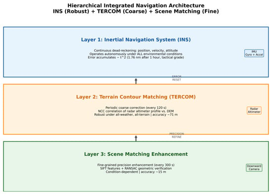
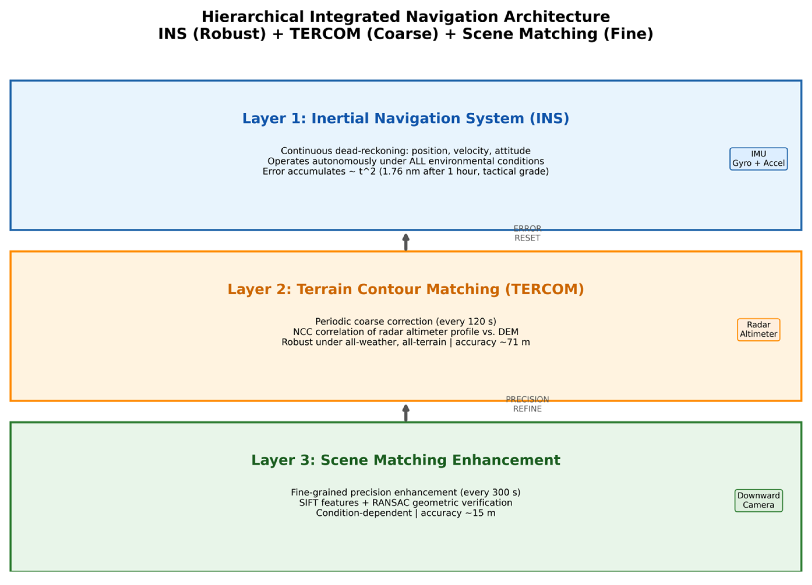
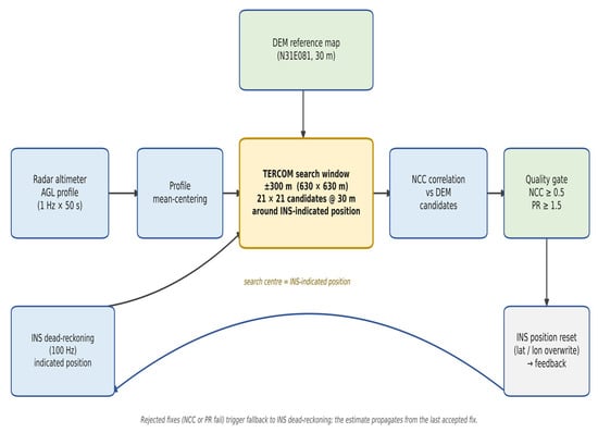
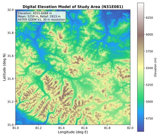
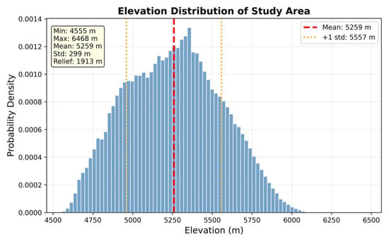
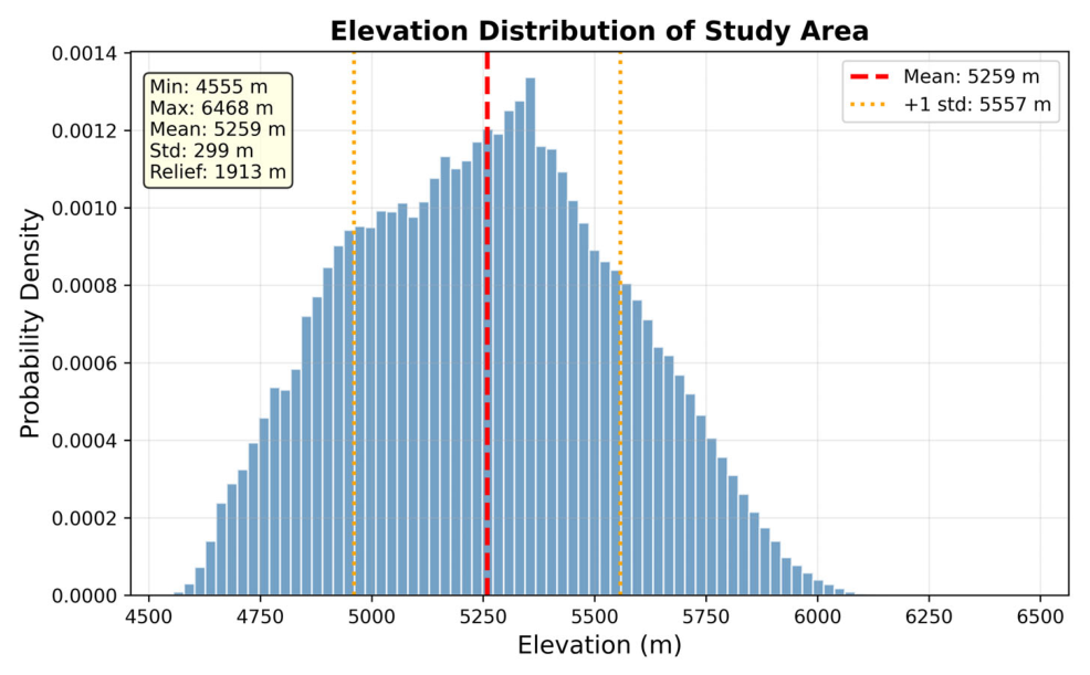
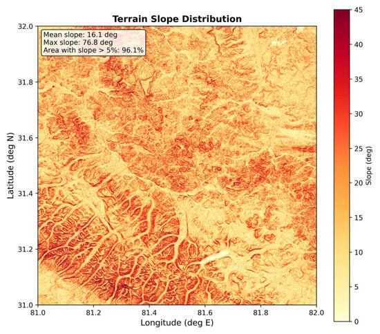
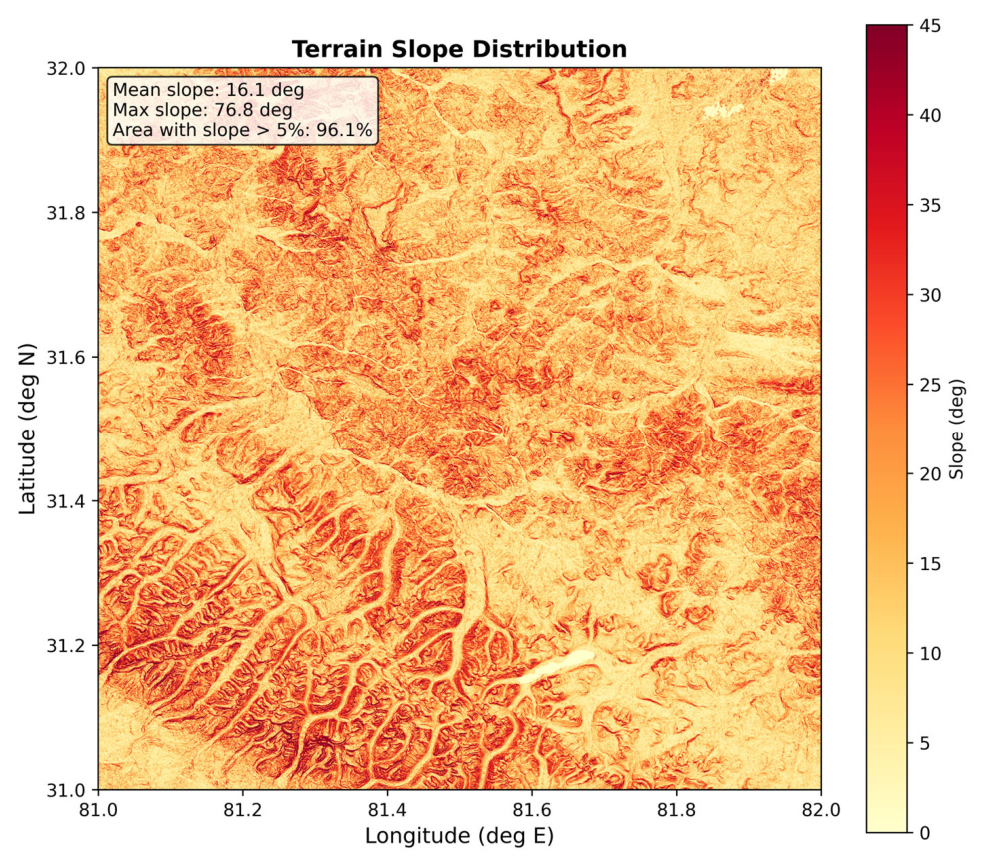
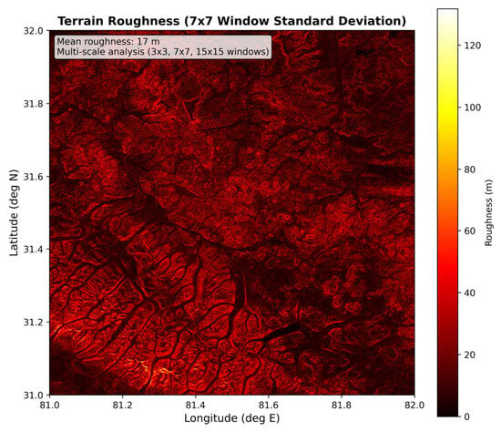
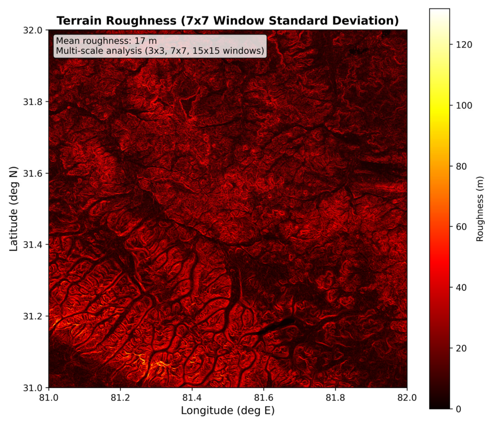
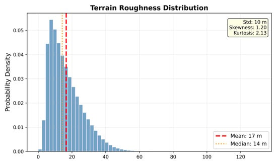
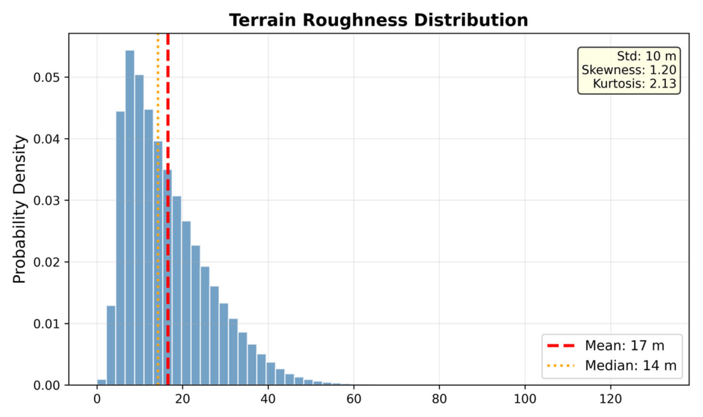
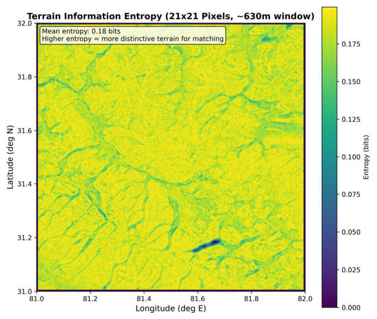
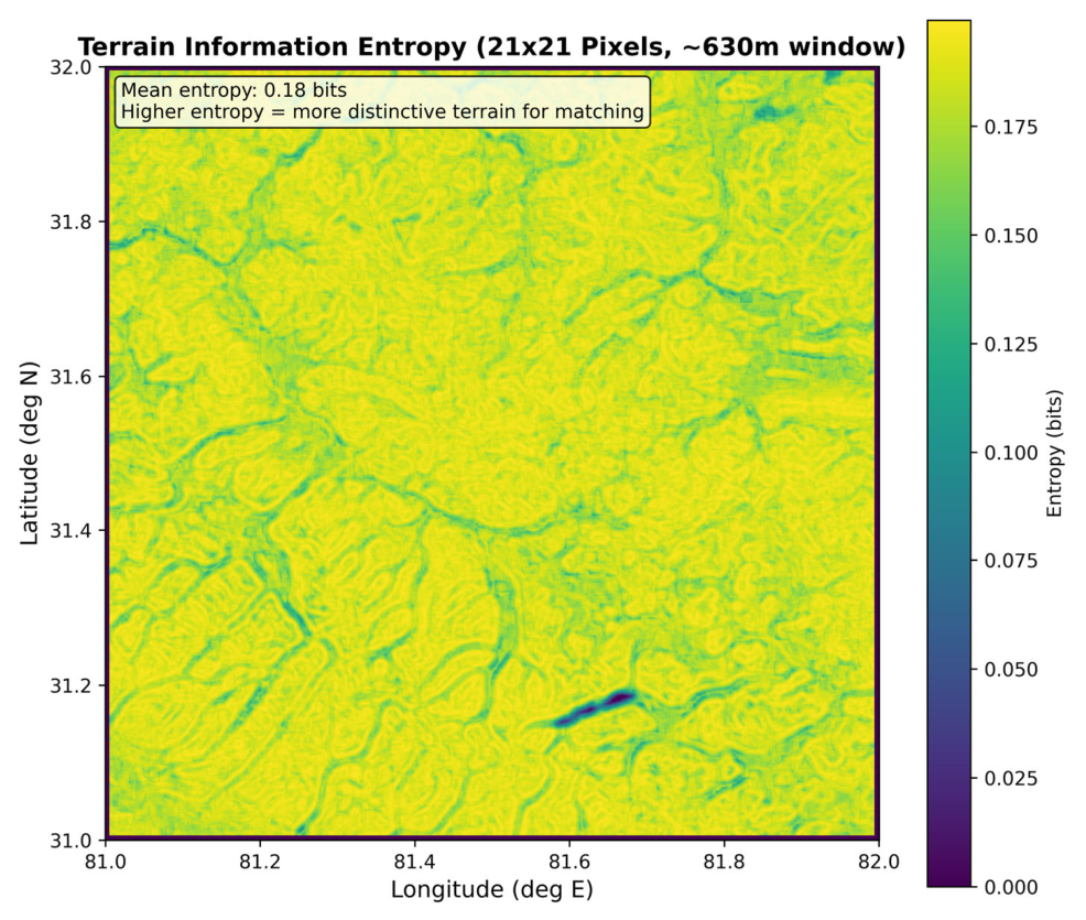
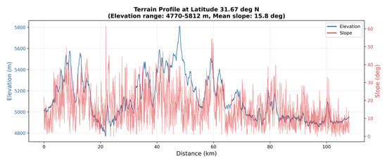
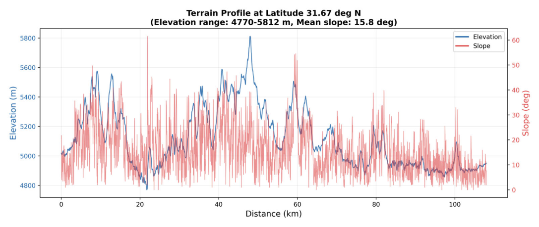
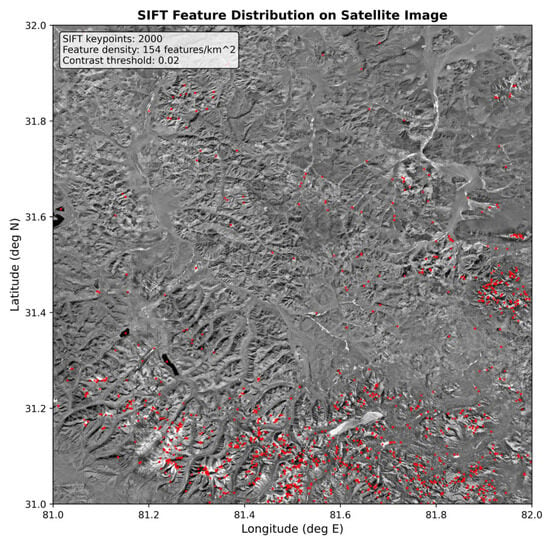
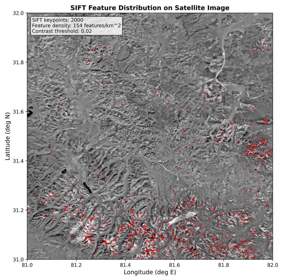
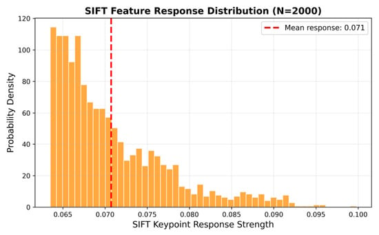
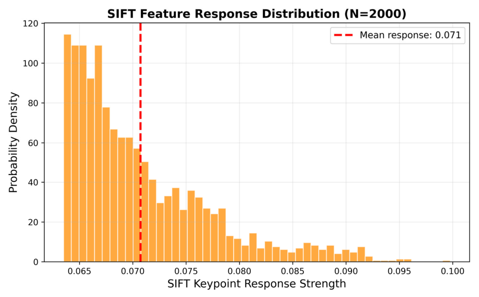
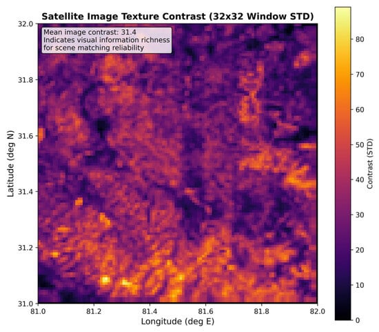
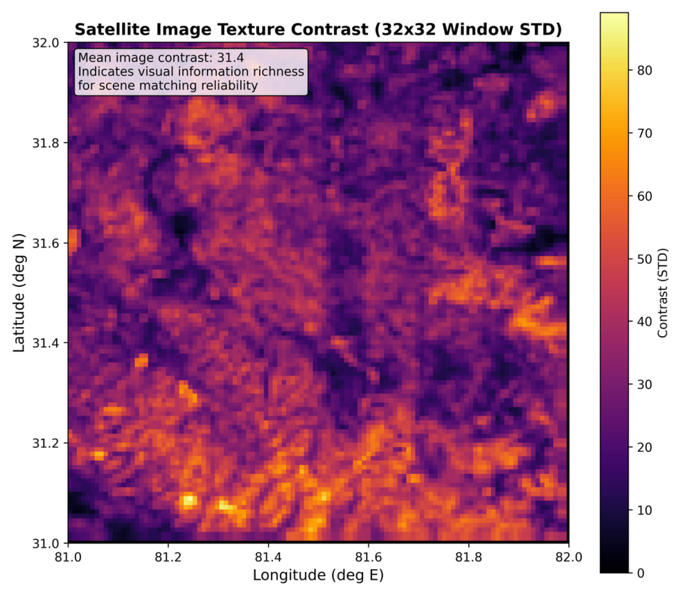
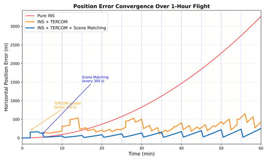
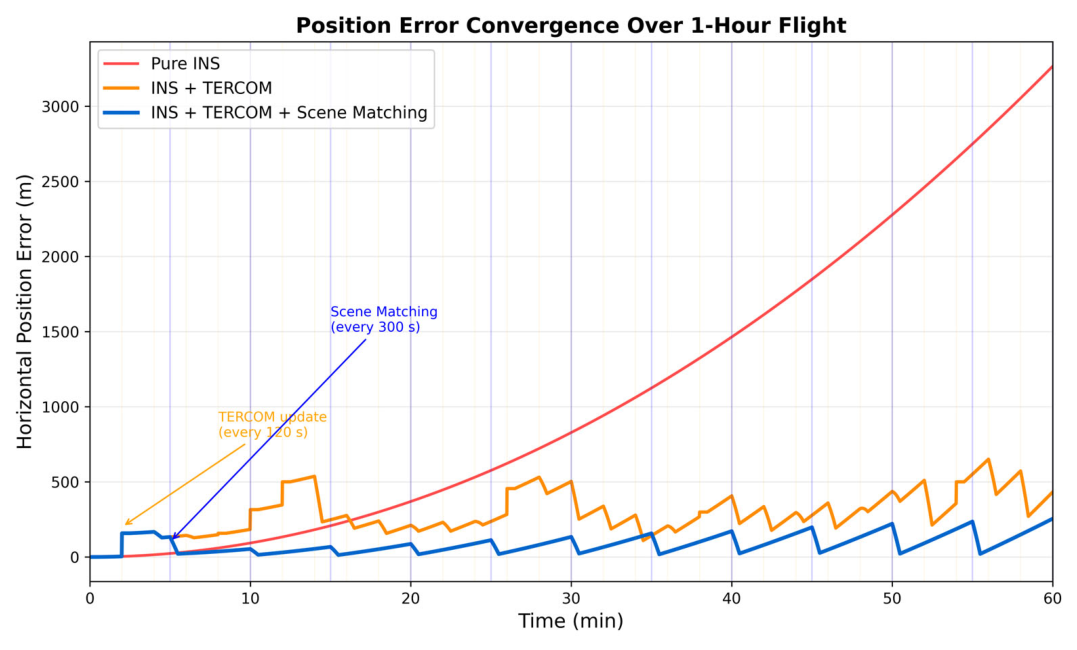
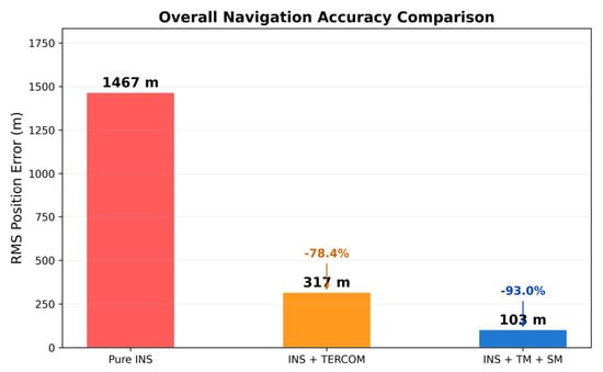
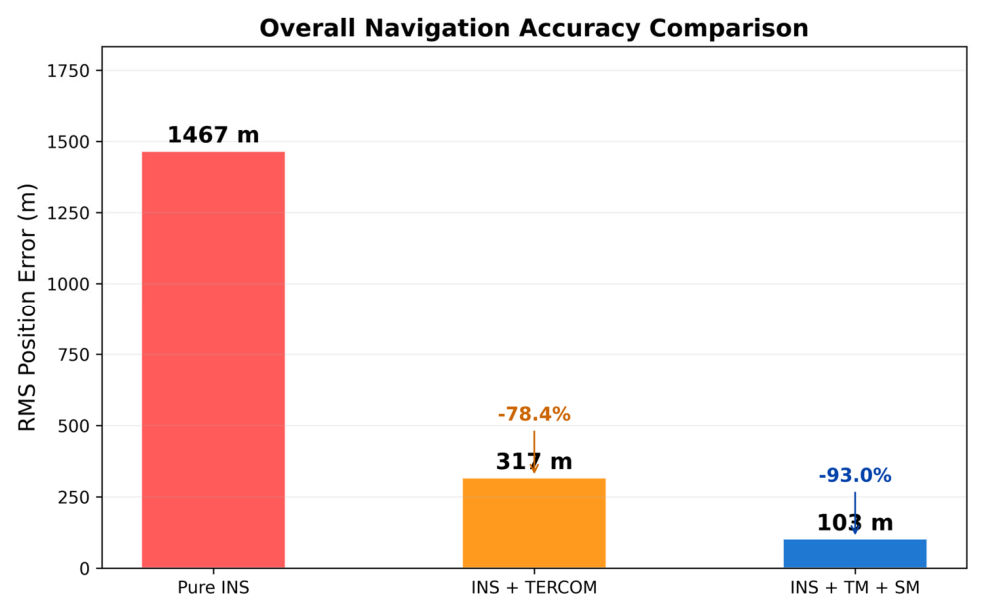
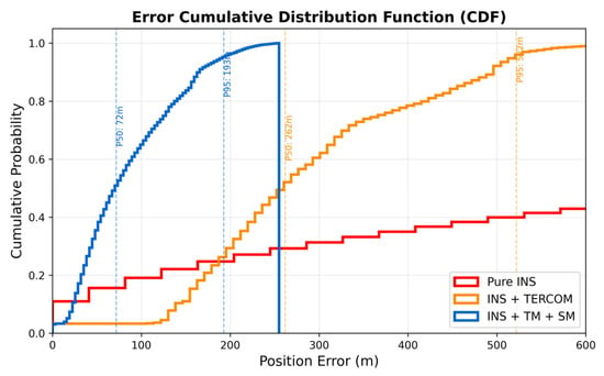
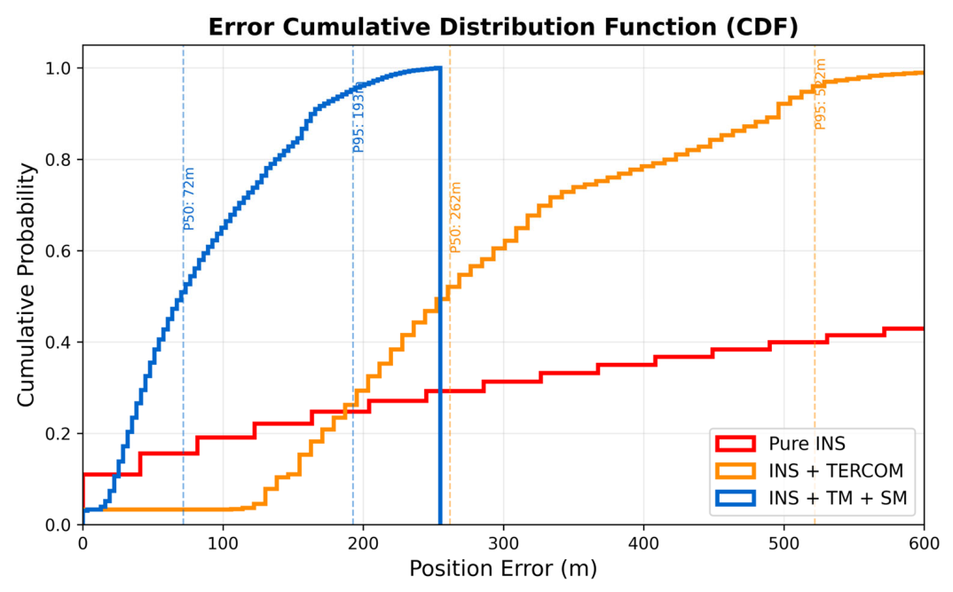
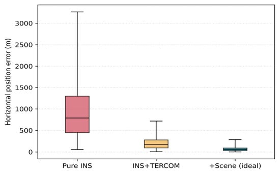
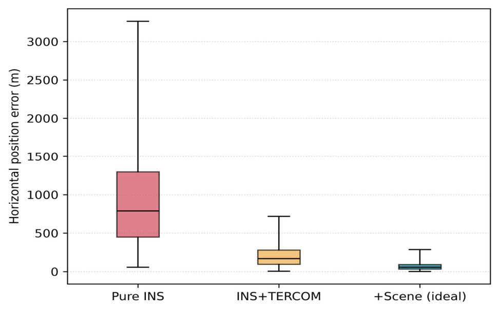
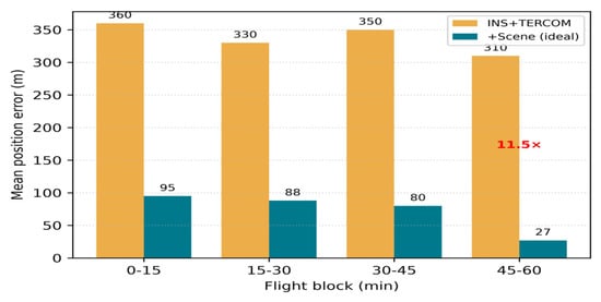
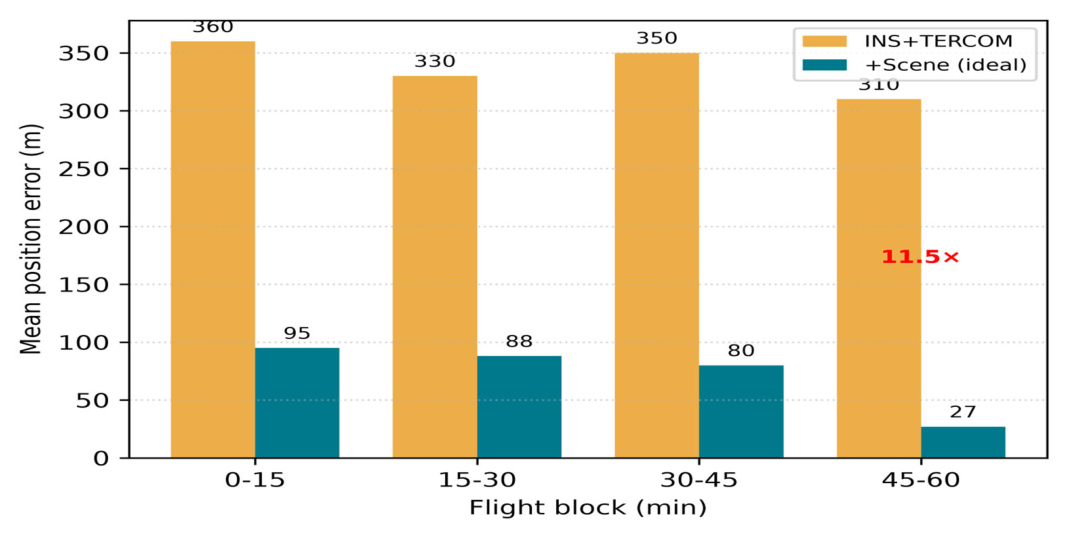
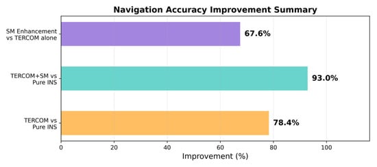
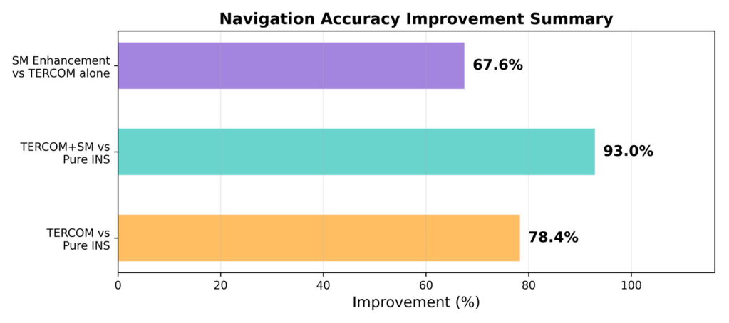
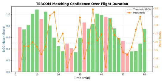
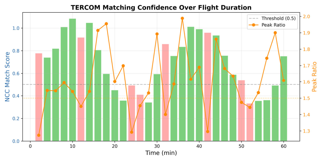
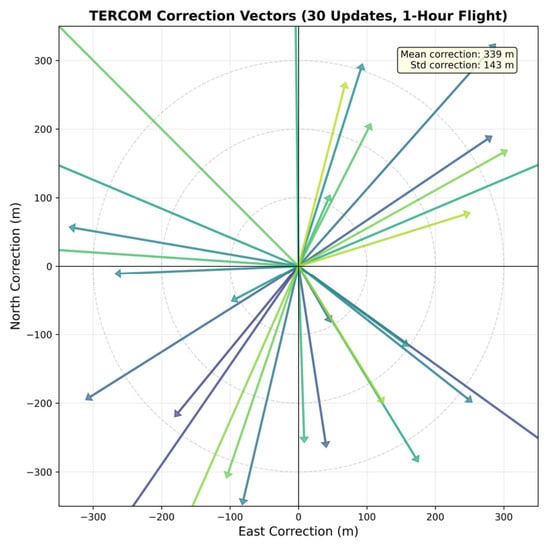
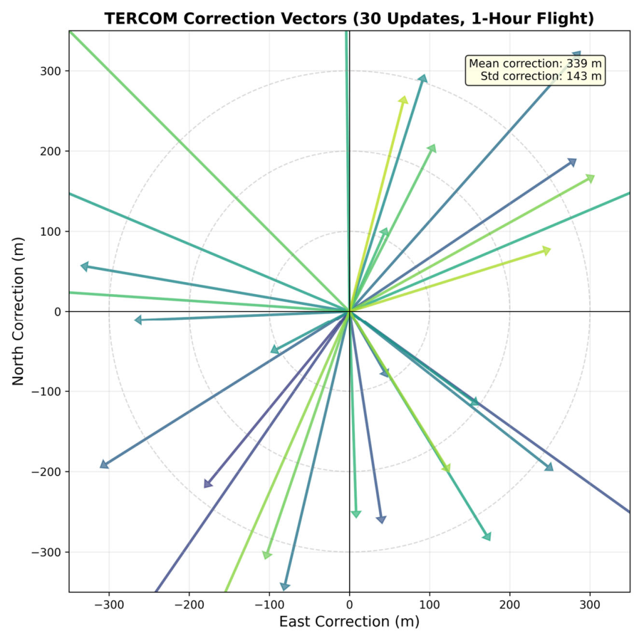

Disclaimer/Publisher’s Note: The statements, opinions and data contained in all publications are solely those of the individual author(s) and contributor(s) and not of MDPI and/or the editor(s). MDPI and/or the editor(s) disclaim responsibility for any injury to people or property resulting from any ideas, methods, instructions or products referred to in the content. |
© 2026 by the authors. Licensee MDPI, Basel, Switzerland. This article is an open access article distributed under the terms and conditions of the Creative Commons Attribution (CC BY) license.