Validation-Aware Surrogate Shortlisting for Biomedical Microwave Imaging: Analytical Performance and FDTD Transfer

Abstract

Broadband antenna, frequency and channel selection requires efficient prioritisation of finite candidate configurations, yet strong surrogate performance within a simplified analytical model does not ensure that the learned ordering will transfer to another electromagnetic representation. This study developed a validation-aware surrogate-shortlisting framework using a controlled breast-mimetic benchmark comprising 120 scenarios and 80 antenna–frequency–channel candidates per scenario. Surrogate models were developed using grouped scenario-level validation, and the model and five-candidate shortlist policy were frozen before external evaluation. Random forest produced the lowest-regret analytical-domain shortlist and remained stable across model-initialisation seeds. The frozen ranking was then challenged on held-out scenarios using a separately implemented restricted two-dimensional transverse-magnetic finite-difference time-domain model. Although numerical-reference checks supported shortlist-level use of the operational grid, candidate ordering did not transfer reliably: optimum inclusion, shortlist agreement and rank association were weak, although a qualified candidate within 2 mm of the finite-library FDTD optimum was retained in 58.3% of cases. Transfer failure varied by frequency band and channel family, while incomplete alignment between the analytical and FDTD candidate libraries prevented attribution of the discrepancy to electromagnetic-model shift alone. The framework therefore positions analytical surrogates as auditable shortlisting tools that reduce downstream candidate-level assessment while retaining independent electromagnetic evaluation before final design selection.

1. Introduction

Broadband antenna-array and interrogation design requires comparison of numerous configurations defined by antenna placement, sensing distance, frequency coverage and transmit–receive channel selection. In microwave and radiofrequency sensing, the relative performance of these configurations may also depend on tissue composition, dielectric contrast, target location and background heterogeneity. Exhaustive evaluation can therefore become computationally demanding when each candidate requires detailed electromagnetic simulation, reconstruction or experimental measurement. Surrogate modelling offers a practical alternative by learning relationships between candidate descriptors and design outcomes, thereby allowing promising configurations to be prioritised for further assessment [1,2,3,4].

Microwave breast imaging provides a demanding benchmark because lesion-associated responses are generally weak relative to the heterogeneous background and are sensitive to frequency, propagation path, antenna geometry, tissue organisation, skin-layer effects, dispersion, dielectric variability and coupling conditions. Previous studies have investigated ultra-wideband antennas, Vivaldi arrays, multistatic acquisition and microwave-imaging approaches for breast-mimetic applications [5,6,7,8,9,10,11]. In the present study, this setting is used as a controlled RF system-design benchmark rather than as evidence of clinical diagnostic performance.

Surrogate-assisted optimisation has been applied widely to antennas, microwave devices and electromagnetic components [12,13,14,15], while more recent electromagnetic AI studies have explored physics-informed surrogates, equation-constrained learning and deep-learning-enabled inverse design [12,13,14,15,16,17,18,19,20]. However, most evaluations are conducted within the same analytical or numerical representation used for model development. Such testing can establish predictive consistency and ranking performance within that representation, but it cannot determine whether the learned candidate preferences remain useful when heterogeneous propagation, dispersion, boundary interactions, phase behaviour or reconstruction responses are represented differently.

This distinction is particularly important for finite-candidate shortlisting, in which a surrogate ranks a predefined library and forwards only the top $K$ configurations for detailed evaluation. Its practical value depends on whether the shortlist retains a qualified candidate close to the best available option; regret, optimum inclusion, shortlist overlap and rank association are therefore more informative decision-level endpoints than prediction error alone.

The present model is descriptor-based: its inputs represent frequency design, channel family, candidate geometry, tissue organisation and material properties, but it does not embed Maxwell equations, electromagnetic residuals, a neural field operator or a finite-antenna solver. Although physically motivated descriptors may improve transparency and support learning within a controlled generator, they do not make the resulting ranking representation-independent. Accordingly, the methodological contribution is not a new learning architecture but a validation-aware external-evaluation framework in which the feature scope, model family, ranking rule and shortlist budget are frozen within the analytical generator before being challenged on held-out biological scenarios using a separately implemented restricted 2-D ${\mathrm{T}\mathrm{M}}_z$ FDTD representation. In the first stage, a controlled breast-mimetic analytical benchmark comprising 120 scenarios and 80 finite antenna–frequency–channel candidates per scenario is used to develop surrogate models through grouped scenario-level validation. A representative antipodal Vivaldi element and a 16-position, two-ring sensing arrangement define the analytical design context, and a five-candidate shortlist policy is frozen before external evaluation. The second stage tests whether this ranking retains decision value under the restricted FDTD representation, which uses ideal in-plane sources and receivers and therefore evaluates restricted electromagnetic transfer rather than complete finite-antenna or hardware performance.

The study contributes a controlled finite-candidate RF design benchmark with scenario-level leakage control; regret-first surrogate development and model-seed stability assessment; shortlist-level numerical-reference evaluation of the operational FDTD grid; explicit auditing of analytical–FDTD candidate-support alignment; held-out transfer analysis using regret, optimum inclusion, shortlist overlap, rank association and localisation ambiguity; and structured interpretation of transfer failure by frequency band and channel family. Its intended outcome is a framework for determining when an analytical surrogate can provide a provisional shortlist and when independent electromagnetic evaluation remains necessary before final configuration selection. It is not intended to provide a clinically validated microwave breast-imaging system or to replace three-dimensional finite-antenna simulation.

2. Materials and Methods

2.1. Study Overview and Staged Validation Design

This study developed and evaluated a surrogate-ranking framework for antenna-array, frequency and channel selection under a finite evaluation budget in a controlled breast-mimetic RF benchmark. The evaluation comprised two stages. First, a seed-controlled analytical generator was used to construct reproducible candidate-ranking tasks, develop the surrogate models and prospectively fix a finite-candidate shortlisting policy. Second, the selected surrogate was challenged using a separately implemented restricted two-dimensional $T{M}_z$ finite-difference time-domain model. The biological scenario was treated as the independent unit for model development and statistical inference because candidates from the same scenario shared tissue organisation, material properties and lesion characteristics. Candidate records were therefore treated as nested evaluations rather than independent biological samples.

The benchmark comprised 120 biological scenarios and 80 analytical candidates per scenario, yielding 9600 scenario–candidate records. Of the 120 scenarios, 105 were assigned to grouped analytical development, three to numerical-reference assessment and 12 to held-out FDTD evaluation. Six held-out scenarios were fixed before inspection of their FDTD outcomes. Six additional stress scenarios were selected from the remaining eligible pool by deterministic maximin sampling based on lesion diameter, fibroglandular fraction, tissue-organisation correlation length and radial lesion distance. After standardisation within the eligible pool, each additional scenario was selected to maximise its minimum squared Euclidean distance from those already retained; the three remaining eligible scenarios were reserved for numerical-reference assessment.

No FDTD outcome informed feature-scope selection, model-family selection, hyperparameter specification, shortlist-budget selection, scenario replacement or endpoint definition. The analytical stage evaluated candidate ranking within the controlled generator, whereas the held-out FDTD stage assessed whether the prospectively fixed ranking retained decision value under a distinct electromagnetic representation.

2.2. Breast-Mimetic Benchmark, Sensing Geometry and Candidate Parameterisation

The analytical benchmark represented a hemispherical breast-mimetic domain with radius $R_b=60$ mm and a 2 mm skin-like outer layer. These dimensions are consistent with hemispherical and layered breast-phantom configurations reported in microwave-imaging studies [5,6,7,8,9,10,11,21] and were selected to provide a reproducible geometry rather than to represent the full anatomical variability of the human breast. Internal heterogeneity was represented using adipose-like and fibroglandular-like tissue classes. In this study, fibroglandular fractions ranged from 10% to 40%, and tissue-organisation correlation lengths ranged from 8 to 12 mm. The fibroglandular fraction controlled tissue-class occupancy, whereas the correlation length controlled spatial clustering. Each FDTD cell retained one tissue-class assignment; no Maxwell–Garnett, Bruggeman or other effective-medium mixing rule was applied at the cell level.

Each scenario contained one lesion-like inclusion with diameter $a\in \left\{5,10,15\right\} \mathrm{m}\mathrm{m}.$ Lesion position, depth, dielectric contrast, tissue properties and background organisation varied across scenarios to create controlled differences in localisation difficulty. These parameter ranges were not intended to reproduce a clinical population distribution.

For each biological scenario, 80 finite array–frequency–channel candidates were generated within a fixed 16-position, two-ring analytical framework. The candidates represented alternative interrogation configurations obtained by varying antenna-to-surface distance, relative ring offset, frequency subset, centre frequency, bandwidth and transmit–receive channel family; they did not represent distinct antenna elements.

The 3–8 GHz interval was selected as a bounded ultra-wideband evaluation envelope overlapping frequency ranges used in previous Vivaldi and multistatic microwave breast-imaging studies [5,6,10,11]. The interval included lower-frequency components expected to provide greater penetration and upper-frequency components expected to provide finer spatial sensitivity, while allowing the increased attenuation and sensitivity to tissue heterogeneity associated with the upper part of the band to be examined within a common candidate library. It enabled controlled comparison of lower-, intermediate- and upper-frequency subsets and was not assumed to be universally optimal.

In this study, antenna-to-surface distance varied from 5 to 20 mm in the analytical benchmark. This deliberately broad range was used only as an analytical design variable to determine whether the generator assigned different preferences across sensing distances; it was not supported by loaded-antenna matching calculations or finite-antenna simulations. The held-out FDTD challenge was therefore restricted to stand-offs of 15 and 20 mm, consistent with separations used in reported 16-element breast-imaging configurations [22,23]. No inference was made regarding realised antenna matching, radiation efficiency or usable bandwidth at stand-offs of 5 or 10 mm.

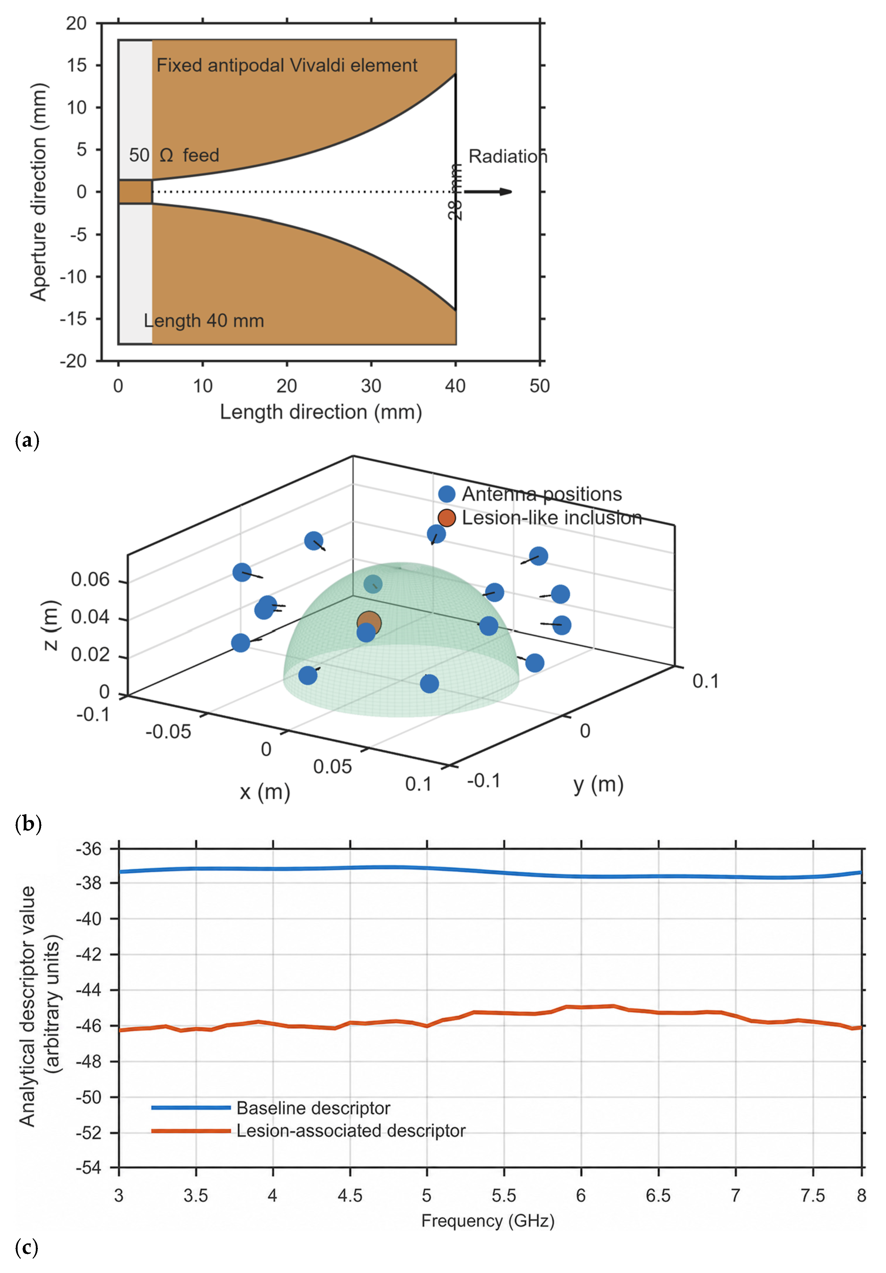
An antipodal Vivaldi antenna provided the broadband context for analytical candidate parameterisation but was not simulated as a finite port-driven antenna. The nominal assumptions used in this study were a 3–8 GHz operating range, a 50 $\mathsf{\Omega }$ feed impedance, a 40 mm antenna length, a 28 mm aperture width, a substrate relative permittivity of 3.55, a substrate thickness of 0.813 mm and a metallisation thickness of 35 μm. Linear polarisation directed towards the breast-mimetic domain was assumed. A nominal condition of $S_{11,\mathrm{d}\mathrm{B}}<-10$ dB defined the intended useful band but was not treated as a simulated or measured antenna result.

Figure 1 illustrates the representative Vivaldi element, 16-position, two-ring geometry and analytical descriptor profiles; the geometry was not intended to represent a coupling-qualified finite-antenna array. For ring $r\in \left\{1,2\right\}$ and position $i\in \left\{1,\dots ,8\right\}$,

$$p_{r,i}=\left[\begin{array}{c}\left(R_b+d\right)\cos {\varphi }_{r,i}\\ \left(R_b+d\right)\sin {\varphi }_{r,i}\\ z_r\end{array}\right],{\varphi }_{r,i}={\displaystyle \frac{2\pi \left(i-1\right)}{8}}+{\theta }_r$$

where $d$ is the antenna-to-surface distance, $z_r$ is the axial ring position and ${\theta }_r$ is the ring offset. The analytical frequency grid was defined as

$$f_k=f_{\mathrm{m}\mathrm{i}\mathrm{n}}^{\left(\mathrm{g}\mathrm{r}\mathrm{i}\mathrm{d}\right)}+\left(k-1\right)\Delta f,k=1,\dots ,N_{\nu }.$$

In this study,

$$f_{\mathrm{m}\mathrm{i}\mathrm{n}}^{\left(\mathrm{g}\mathrm{r}\mathrm{i}\mathrm{d}\right)}=3 \mathrm{G}\mathrm{H}\mathrm{z},\Delta f=0.1 \mathrm{G}\mathrm{H}\mathrm{z},N_{\nu }=51$$

giving a uniform grid from 3 to 8 GHz. For candidate $c$, the selected frequency subset $F_c$ was characterised by the number of selected frequencies $N_f$, lower frequency $f_{\mathrm{m}\mathrm{i}\mathrm{n}}$, upper frequency $f_{\mathrm{m}\mathrm{a}\mathrm{x}}$, centre frequency $f_c={\displaystyle \frac{f_{\mathrm{m}\mathrm{i}\mathrm{n}}+f_{\mathrm{m}\mathrm{a}\mathrm{x}}}{2}},$ and bandwidth $B=f_{\mathrm{m}\mathrm{a}\mathrm{x}}-f_{\mathrm{m}\mathrm{i}\mathrm{n}}.$

Five analytical channel families were considered: adjacent, skip-one, opposite, inter-ring and full multistatic. Restricting selection to predefined families avoided an unconstrained channel search while retaining differences in channel diversity. Full multistatic denoted all eligible transmit–receive pairs within the analytical framework and did not imply validated matching, isolation, mutual-coupling or loaded-radiation-pattern performance for a fabricated array. No coupling-derived minimum element separation or multiport $S_{mn}$ threshold was imposed because the 16 positions defined an analytical sensing geometry rather than a simulated finite-antenna array. The benchmark therefore represented a controlled finite-candidate RF design problem rather than a validated finite-antenna or clinical imaging system.

2.3. Controlled Analytical Benchmark Generator and Ranking Endpoint

For biological scenario $s$ and candidate $c$, the complete input vector was denoted as $x_{s,c}\in {\mathbb{R}}^p$, where $p=26$ in this study. The subset entering the analytical endpoint generator was

$$x_{s,c}^{\left(g\right)}={\left[d,\theta ,N_f,f_c,B,{\chi }_c^T,h,a,z_d,C\right]}^T\in {\mathbb{R}}^{p_g}$$

where $p_g=14$ in this study. Here, ${\chi }_c\in {\left\{0,1\right\}}^5$ is the one-hot channel-family indicator, $h$ is the fibroglandular fraction, $a$ is lesion diameter, $z_d$ is lesion depth and $C$ is the dielectric-contrast ratio. Conductivity and tissue-correlation-length variables were retained in the complete input vector for feature-scope analysis but did not enter the analytical endpoint equations directly; tissue-permittivity variables contributed through $C$.

The generator encoded prespecified qualitative relationships rather than approximating an electromagnetic forward solution. Within the benchmark, larger lesion diameter and dielectric contrast increased analytical detectability, whereas greater lesion depth and fibroglandular fraction increased scenario difficulty. Candidate performance varied smoothly around scenario-dependent preferred values of centre frequency, bandwidth and stand-off distance. These relationships defined the ranking task but were not interpreted as experimentally calibrated electromagnetic laws.

Clipping to a finite interval was defined as ${\mathcal{C}}_{\left[l,u\right]}\left(x\right)=\mathrm{m}\mathrm{i}\mathrm{n}\{\mathrm{m}\mathrm{a}\mathrm{x}\left(x,l\right),u\}$. Candidate compatibility was represented by $S_{s,c}={\left[S_f,S_d,S_N,S_{\theta },S_{\mathrm{c}\mathrm{h}}\right]}^T$, where the components represented frequency-design, stand-off, frequency-count, angular-offset and channel-family compatibility, respectively. Smooth functions were used to avoid discontinuous candidate-preference boundaries, and channel-family weights were fixed benchmark-construction constants rather than measured antenna characteristics.

Analytical field-coverage, detectability, localisation-sensitivity and robustness scores followed the common form

$$Y_{j,s,c}={\mathcal{C}}_{\left[l_j,u_j\right]}\left({\beta }_{j,0}+{\beta }_j^T{v}_{j,s,c}+{\xi }_{j,s,c}\right),j\in \left\{F,D,L,Q\right\}$$

where $v_{j,s,c}$ contains the variables entering score $j$, ${\beta }_{j,0}$ and ${\beta }_j$ are prespecified coefficients, and ${\xi }_{j,s,c}$ is record-specific, seed-controlled benchmark variation. Recoverability was defined as

$$R_{s,c}={\mathcal{C}}_{\left[R_{\mathrm{m}\mathrm{i}\mathrm{n}},R_{\mathrm{m}\mathrm{a}\mathrm{x}}\right]}\left(D_{s,c}^{\hspace{0.17em}{r}_D}{L}_{s,c}^{\hspace{0.17em}{r}_L}{Q}_{s,c}^{\hspace{0.17em}{r}_Q}\right)$$

A composite utility $U_{s,c}$ combined localisation sensitivity, recoverability, detectability, field coverage and robustness using fixed weights. A separate scenario-difficulty term $G_s$ increased with smaller lesion diameter, greater lesion depth, greater fibroglandular fraction and lower dielectric contrast. The primary analytical ranking endpoint was

$$E_{s,c}^{\mathrm{l}\mathrm{o}\mathrm{c}}={\mathcal{C}}_{\left[E_{\mathrm{m}\mathrm{i}\mathrm{n}},E_{\mathrm{m}\mathrm{a}\mathrm{x}}\right]}\left({\eta }_0-{\eta }_U{U}_{s,c}+{\eta }_G{G}_s+{\xi }_{s,c}^E\right)$$

The analytical localisation-error label was generated directly from these benchmark rules rather than from an electromagnetic-field solution or the maximum of a Maxwell-derived localisation image. The generator also returned a frequency-dependent analytical vector

$${\mathsf{\ell }}_{s,c}={\left[{\mathsf{\ell }}_{s,c},\left(f_1\right),{\mathsf{\ell }}_{s,c},\left(f_2\right)\dots {\mathsf{\ell }}_{s,c}\left(f_{N_{\nu }}\right)\right]}^T\in {\mathbb{R}}^{N_{\nu }}$$

where $N_{\nu }=51$ in this study. This vector provided reproducible frequency-dependent structure but was not interpreted as a calibrated scattering parameter, complex electromagnetic response or measured spectrum.

Appendix A reports the complete functional forms, numerical coefficients, normalisation rules, clipping bounds, channel weights, random-seed rules and baseline settings used in this study. All generator parameters were fixed before surrogate development and were neither estimated from measurements nor fitted or calibrated to the held-out FDTD outcomes. The resulting quantities were therefore interpreted as ranking variables within the analytical benchmark rather than estimates of electromagnetic-system performance.

2.4. Surrogate Development, Model Selection and Interpretability

Each surrogate predicted candidate-level analytical localisation error, after which candidates were ranked in ascending order of predicted error within each biological scenario. The primary surrogate input comprised $p_{\mathrm{p}\mathrm{r}\mathrm{i}\mathrm{m}\mathrm{a}\mathrm{r}\mathrm{y}}$ target-agnostic variables available before candidate reconstruction or response evaluation, where $p_{\mathrm{p}\mathrm{r}\mathrm{i}\mathrm{m}\mathrm{a}\mathrm{r}\mathrm{y}}=21$ in this study. These variables represented candidate geometry, frequency design, channel family, tissue organisation and background dielectric and conductivity properties. Five privileged variables—lesion permittivity, lesion conductivity, lesion diameter, lesion depth and dielectric-contrast ratio—were excluded from the primary scope because they would not ordinarily be available during prospective candidate selection. Reinstating these variables produced the oracle-assisted scope, for which $p_{\mathrm{o}\mathrm{r}\mathrm{a}\mathrm{c}\mathrm{l}\mathrm{e}}=26$ in this study. The oracle-assisted scope was used only to quantify the effect of privileged scenario information and was treated as a methodological upper bound. Generated response and performance quantities were excluded from both scopes.

Ridge regression, random forest, boosted trees and a random-ranking baseline were compared using grouped five-fold cross-validation repeated three times. All candidates from one biological scenario remained within the same fold. Within each repeat, the five validation folds were disjoint, and each of the 105 analytical-development scenarios appeared in validation exactly once. Fold assignments were reshuffled between repeats; each scenario therefore appeared in validation once per repeat and three times across the complete repeated-validation procedure. Validation sets were disjoint within each repeat but not across repeats. Data transformation, standardisation and model fitting were performed using the training portion of each fold and applied unchanged to the corresponding validation portion.

The model configurations were fixed before held-out FDTD evaluation. Ridge regression used a regularisation parameter of ${10}^{-2}$. Random forest used bootstrap aggregation with 250 regression trees, a minimum leaf size of 5 and surrogate splits disabled. Boosted trees used least-squares boosting with 300 learning cycles, a learning rate of 0.05, a minimum leaf size of 8 and surrogate splits disabled. Random rankings were generated using reproducibly seeded within-scenario permutations. The model-development seed was 20260729; the separate analytical-generator seed is reported in Appendix A. These settings supported reproducible comparisons rather than exhaustive hyperparameter optimisation.

Two scenario-independent candidate templates were defined identically in every analytical scenario, a 10 mm stand-off template and a 15 mm stand-off template, each using the full 3–8 GHz band and full multistatic acquisition. These templates were evaluated at $K=1$ as global comparators against scenario-conditioned random-forest ranking. The remaining candidate identifiers represented scenario-specific generated designs and were therefore not treated as universally shared configurations.

For the surrogate models, candidate budgets of $K\in \left\{1,3,5,10,20\right\}$ were evaluated analytically, with $K=5$ prospectively designated as the primary shortlist budget before restricted-FDTD evaluation. Model selection followed a prespecified sequential rule: the model with the lowest mean best-in-shortlist regret was selected first; oracle recall was considered only when mean regret did not distinguish the models; and top-$K$ overlap was considered only when the preceding criteria remained unresolved. No FDTD outcome entered feature-scope selection, model selection, hyperparameter specification or shortlist-budget determination.

A 20-run fixed-partition stability analysis was performed for random forest and boosted trees. The grouped folds, primary input scope, preprocessing rules, hyperparameters and $K=5$ budget remained fixed, while only the model-initialisation seed varied. These runs assessed algorithmic sensitivity and were not treated as additional biological scenarios or independent datasets.

Grouped permutation importance was evaluated using the model selected by the prespecified analytical rule and the primary $K=5$ shortlist budget. Six feature groups were considered: frequency design, channel family, candidate geometry, tissue organisation, background conductivity and background dielectric properties. Each group was permuted over 30 iterations, and importance was defined as the resulting increase in scenario-level five-candidate regret relative to the unpermuted model. Leave-one-feature-group-out retraining provided a complementary assessment using the same grouped partitions, preprocessing rules and model settings. Oracle-assisted results were interpreted only as a methodological upper bound. These analyses assessed predictive dependence on feature groups and were not interpreted as causal physical effects.

2.5. Restricted Held-Out Two-Dimensional $T{M}_z$ FDTD Challenge

The prospectively fixed analytical surrogate was challenged using a separately implemented two-dimensional $T{M}_z$ FDTD model. Candidate rankings were generated without access to the corresponding FDTD outcomes. The FDTD domain and restricted candidate structure followed

Table 1. Relationship between the analytical benchmark and the restricted FDTD challenge.

Component	Analytical Benchmark and Surrogate Development	Restricted FDTD Challenge
Breast-mimetic representation	Hemispherical design domain with 60 mm radius and 2 mm skin-like layer	2-D ${\mathrm{T}\mathrm{M}}_z$ in-plane cross-section with 60 mm radius and 2 mm skin layer
Scenario use	105 scenarios for grouped development after exclusions	Three numerical-reference scenarios and 12 held-out scenarios
Radiating-element representation	Representative antipodal Vivaldi element within a 16-position two-ring design framework	Sixteen ideal in-plane source and receiver positions; no finite antenna geometry
Candidate support	80 array–frequency–channel candidates per scenario	40 candidates per scenario: 20 at each of two stand-offs
Frequency parameterisation	Fifty-one samples over 3–8 GHz and candidate-specific frequency subsets	Five bands: 3–5, 3–8, 4–6, 5–7 and 6–8 GHz
Channel parameterisation	Adjacent, skip-one, opposite, inter-ring and full-multistatic families	Adjacent, skip-one, opposite and in-plane full-multistatic families
Primary shared endpoint	Candidate localisation error within the analytical benchmark	Candidate localisation error reconstructed from FDTD responses
Role	Surrogate development, model selection and within-generator evaluation	Independent evaluation of frozen shortlist transfer

. Sixteen ideal in-plane source and receiver positions surrounded the breast cross-section, and a fixed spatial-organisation field assigned adipose-like or fibroglandular-like material to each interior cell.

For each scenario, stand-off and transmitter, matched lesion-present and lesion-absent simulations were performed. In the lesion-present state, the background material within the prescribed circular lesion region was replaced by lesion-like tissue, whereas the lesion-absent state retained the original tissue assignment. Geometry, tissue organisation, excitation and numerical settings were otherwise identical, and the complex frequency-domain responses from the two states were differenced before reconstruction.

Candidate ranking and evaluation were performed separately within each 20-candidate scenario–stand-off unit. The same reconstruction procedure and imaging domain were used for all candidates. Target position was estimated using a log-quadratic subpixel fit around the strongest reconstructed peak, while the discrete-grid maximum was retained as a secondary diagnostic. The reconstruction-image spacing was 2 mm.

Frequency-dependent material properties were represented using the single-pole Debye model

$${\epsilon }^{*}\left(\omega \right)={\epsilon }_{\infty }+{\displaystyle \frac{\Delta \epsilon }{1+j\omega \tau }}-{\displaystyle \frac{j{\sigma }_s}{\omega {\epsilon }_0}}$$

where ${\epsilon }^{*}$ is the complex relative permittivity, ${\epsilon }_{\infty }$ is the infinite-frequency relative permittivity, $\Delta \epsilon$ is the relaxation strength, $\tau$ is the relaxation time, ${\sigma }_s$ is the static-conductivity term, ${\epsilon }_0$ is the vacuum permittivity and $\omega$ is the angular frequency.

Frequency-dependent FDTD tissue properties were obtained from a fixed table derived from published dielectric measurements and parametric models. Skin values were based on the Gabriel tissue data [24,25]; adipose-like values were derived from the high-adipose normal-breast group reported by Lazebnik et al. [26]; fibroglandular-like values were derived from the corresponding low-adipose group [26]; and lesion-like values were derived from malignant breast-tissue data [27]. The reference permittivity and conductivity values were tabulated at integer frequencies from 3 to 8 GHz. A positive-parameter single-pole Debye model was fitted to each scenario-specific tissue-property curve before field computation. Across the 480 scenario–material fits used in this study, the maximum normalised root-mean-square fitting error was 0.03985, below the prespecified limit of 0.05. The fitted Debye law was assigned according to the cellwise tissue label; adipose-like and fibroglandular-like properties were not combined using an effective-medium mixing equation. Debye dispersion was applied only in the restricted FDTD evaluation and did not retrospectively redefine the analytical generator as a dispersive electromagnetic model.

The operational grid spacing used in this study was 0.200 mm, the simulation duration was 12 ns, and excitation used a broadband Gaussian-modulated pulse centred at 5.5 GHz. The time step was set to 95% of the two-dimensional Courant–Friedrichs–Lewy limit. The complete tissue-property table, reference Debye fits, scenario-fit criterion, source waveform, grid, time-stepping, boundary, receiver-sampling and reconstruction settings are reported in Appendix B.

The restricted model did not include finite antennas, feed structures, substrates, ports, impedance matching, loaded radiation patterns, cable effects, inter-ring channels, out-of-plane propagation or a complete 16-port mutual-coupling solution. It therefore provided a separate in-plane electromagnetic challenge rather than complete antenna-system, hardware or experimental validation.

2.6. Numerical-Reference Assessment, Transfer Endpoints and Statistical Analysis

The operational grid was compared with a finer numerical grid using three biological scenarios at both stand-offs, yielding six numerical-reference units. In this study, the operational and finer grid spacings were 0.200 and 0.180 mm, respectively. These scenarios were excluded from analytical model development and held-out transfer evaluation, and the finer grid was treated as a numerical comparator rather than exact or fully grid-converged electromagnetic truth.

Let $p_1$ and $p_2$ denote the two highest spatially separated reconstructed peaks, with $p_1\ge p_2$. The normalised peak margin was $m_{\mathrm{p}\mathrm{e}\mathrm{a}\mathrm{k}}={\displaystyle \frac{p_1-p_2}{\mathrm{m}\mathrm{a}\mathrm{x}\left(p_1,ϵ\right)}}$, where $ϵ>0$ is the fixed numerical stabiliser reported in Appendix B. A candidate was classified as localisation-ambiguous when

$$m_{\mathrm{p}\mathrm{e}\mathrm{a}\mathrm{k}}<0.01 \mathrm{and} {∥r_1-r_2∥}_2\ge 4 \mathrm{m}\mathrm{m}$$

where $r_1$ and $r_2$ are the corresponding peak positions. Candidates not meeting this ambiguity condition were considered localisation-qualified.

The relative change in the candidate-used differential response spectrum between the two grids was

$${\Delta }_{\mathrm{s}\mathrm{p}\mathrm{e}\mathrm{c}}\left(\%\right)=100{\displaystyle \frac{{∥\Delta H_{\mathrm{o}\mathrm{p}}-\Delta H_{\mathrm{f}\mathrm{i}\mathrm{n}\mathrm{e}}∥}_2}{\max \hspace{0.17em}\left({∥\Delta H_{\mathrm{f}\mathrm{i}\mathrm{n}\mathrm{e}}∥}_2,ϵ\right)}}$$

where $\Delta H_{\mathrm{o}\mathrm{p}}$ and $\Delta H_{\mathrm{f}\mathrm{i}\mathrm{n}\mathrm{e}}$ are the candidate-used differential response vectors obtained on the operational and finer grids, respectively. The prespecified numerical-reference criteria used in this study required ${\Delta }_{\mathrm{s}\mathrm{p}\mathrm{e}\mathrm{c}}\le 5\%$, best-in-qualified-shortlist regret no greater than 2 mm, qualified top-three overlap of at least $2/3$, at least three qualified candidates on each grid, and at least one operational-grid shortlisted candidate that remained qualified on the finer grid.

Candidate-support alignment was assessed within each biological scenario. Direct comparison of analytical rankings with FDTD outcomes was permitted only when every restricted FDTD candidate had one unique analytical counterpart; approximate and nearest-neighbour substitutions were not used. When complete alignment was unavailable, surrogate predictions and FDTD outcomes were compared over the same restricted candidate pool within each scenario–stand-off unit. This same-support analysis assessed retained shortlist decision value but could not isolate electromagnetic-representation shift from candidate-support shift. Complete numerical-reference and alignment results are reported in

Table A3. Numerical-reference qualification and analytical–FDTD candidate-support audit. (A) Operational-grid qualification; (B) analytical–FDTD candidate-support audit.

(A)
Assessment	Prespecified Criterion	Result	Interpretation
Assessment design	Three independent scenarios evaluated at both stand-offs	Scenarios 85, 91 and 10; 15 and 20 mm; six units	Complete
Grid comparison	0.200 mm operational grid evaluated against a finer numerical comparator	Finer grid: 0.180 mm	Finer grid not treated as exact truth
Reference shortlist	Fixed before numerical-reference evaluation	$K_{ref}=3$	Applied to all six units
Response-spectrum change	$\le 5$% in every unit	Maximum: 1.3035%	Criterion met
Best-in-qualified-shortlist regret	$\le 2$ mm in every unit	Maximum: 0 mm	Criterion met
Qualified top-three overlap	$\ge$2/3 in every unit	Minimum: 0.6667	Criterion met
Candidate availability	At least three qualified candidates on each grid	Minimum: 12 on each grid	Criterion met
Joint shortlist qualification	At least one operational-grid shortlisted candidate also qualified on the finer grid	Minimum: 3	Criterion met
Tissue-map consistency	Fibroglandular-fraction change $\le$0.5 percentage points	Criterion met in all six units	Criterion met
Numerical and accounting controls	Candidate accounting, CPU–GPU agreement, canonical controls and CPML checks required to pass	All controls passed	Criterion met
Overall assessment	Every primary criterion required in all six units	Six of six units met all criteria	0.200 mm grid used for held-out shortlist evaluation
Secondary numerical sensitivity	Retained but not used as a primary criterion	Raw top-one comparator failed; maximum selected-maximum displacement: 2.3384 mm	Exact top-one preservation was not supported
(B)
Assessment	Prespecified Requirement	Result	Interpretation
Audited support	All restricted FDTD candidates assessed within their corresponding biological scenarios	12 scenarios; 40 FDTD candidates per scenario; 480 rows	Complete
Analytical comparison library	Matching against the 80 analytical candidates from the same scenario	960 analytical scenario–candidate rows	Complete
Exact-matching rule	Agreement across all declared design descriptors using a scaled tolerance of ${10}^{-9}$	Matching performed separately within each scenario	Applied as prespecified
Complete support alignment	Every restricted FDTD row required one unique analytical counterpart	Required: 480 of 480 rows	Not achieved
Unique exact matches	Rows with exactly one analytical counterpart	12 of 480 rows (2.5%)	Insufficient for a complete direct matched analytical-to-FDTD comparison
Rows without a unique match	No exact match or more than one exact match	468 of 480 rows (97.5%)	Not used for direct matched comparison
Approximate substitution	Nearest-neighbour or approximate matching not permitted	No substitution performed	Candidate differences were not represented as exact matches
External comparison	Insufficient for a complete matched analytical-to-FDTD comparison	Complete alignment was unavailable	Frozen predictions were compared with FDTD outcomes within the restricted candidate pool
Attribution boundary	Physical-model and candidate-support effects separable only under exact alignment	Effects could not be separated	Transfer gap cannot be attributed solely to solver fidelity

Note for (A): The numerical-reference scenarios were excluded from both surrogate development and held-out transfer evaluation. The 0.180 mm grid was evaluated as a finer numerical comparator and was not treated as exact or fully grid-converged electromagnetic truth. CPU–GPU agreement used a relative tolerance of $5\times {10}^{-4}$. The CPML implementation passed its prespecified checks and used 18 cells at the operational grid; Note for (B): Matching was based on stand-off, angular offset, normalised ring offset, frequency count, lower and upper frequencies, centre frequency, bandwidth and channel-family indicators. Candidate identifiers were not assumed to represent identical designs across libraries. “Same-support” refers to the comparison of surrogate predictions and FDTD outcomes over the same restricted 20-candidate pool within each scenario–stand-off unit; it does not indicate that the restricted FDTD library was an exact subset of the original analytical library.

.

For evaluation unit $u$, let $e\left(u,c\right)$ denote the realised FDTD localisation error of candidate $c$, $S_K\left(u\right)$ the first $K$ candidates ranked by the prospectively fixed surrogate and $C_Q\left(u\right)$ the set of localisation-qualified candidates. When the shortlist contained at least one qualified candidate, best-in-shortlist regret was

$$R_K\left(u\right)=\underset{c\in S_K\left(u\right)\cap C_Q\left(u\right)}{\mathrm{m}\mathrm{i}\mathrm{n}}e\left(u,c\right)-\underset{c\in C_Q\left(u\right)}{\mathrm{m}\mathrm{i}\mathrm{n}}e\left(u,c\right)$$

Values below zero attributable solely to numerical tolerance were set to zero. The qualified finite-library oracle was the candidate in $C_Q\left(u\right)$ with the smallest realised localisation error, and oracle recall was the proportion of evaluation units in which this candidate appeared in $S_K\left(u\right)$.

Let $A_k\left(u\right)$ and $B_k\left(u\right)$ denote the qualified top-$k$ sets obtained from the surrogate and realised FDTD rankings, respectively. Their overlap was

$$O_k\left(u\right)={\displaystyle \frac{\mid A_k\left(u\right)\cap B_k\left(u\right)\mid }{k}}$$

where $k$ was limited by the number of qualified candidates available in both rankings. Qualified top-three and top-five overlap were calculated separately at their respective shortlist sizes. Qualified Spearman association was calculated over localisation-qualified candidates within each scenario–stand-off unit, while shortlist positions occupied by ambiguous candidates remained in the accounting.

When no shortlisted candidate was qualified, penalised regret was

$$R_K^{\mathrm{p}\mathrm{e}\mathrm{n}}\left(u\right)=\max \hspace{0.17em}\left[0,\hspace{0.17em}{e}_{\mathrm{w}\mathrm{o}\mathrm{r}\mathrm{s}\mathrm{t},Q}\left(u\right)-e_{\mathrm{o}\mathrm{r}\mathrm{a}\mathrm{c}\mathrm{l}\mathrm{e}}\left(u\right)\right]$$

where $e_{\mathrm{w}\mathrm{o}\mathrm{r}\mathrm{s}\mathrm{t},Q}\left(u\right)$ and $e_{\mathrm{o}\mathrm{r}\mathrm{a}\mathrm{c}\mathrm{l}\mathrm{e}}\left(u\right)$ are the largest and smallest localisation errors among qualified candidates. When at least one shortlisted candidate was qualified, penalised regret equalled the observed best-in-shortlist regret. The proportion of evaluation units with regret no greater than 2 mm was reported as a practical secondary endpoint, and ambiguity expenditure was defined as the proportion of the five shortlisted positions occupied by localisation-ambiguous candidates.

Analytical metrics were first calculated within each biological scenario before aggregation across folds and repeated validation. Because the three cross-validation repeats reused the same 105 biological scenarios, repeat-level estimates were not treated as independent uncertainty replicates. Confidence intervals for the fixed-template contrasts, grouped-permutation effects and paired random-forest-minus-boosted-tree comparison were estimated using 2000 biological-scenario bootstrap resamples. Biological scenarios were sampled with replacement, while repeated-validation and model-seed observations associated with each sampled scenario remained nested within that scenario cluster and were not treated as independent resampling units. The pairing between compared models or candidate-selection policies was preserved within every resample. Two-sided 95% percentile-bootstrap intervals were reported.

Held-out uncertainty was estimated separately using 2000 biological-scenario cluster-bootstrap resamples. Biological scenarios were sampled with replacement, and both stand-offs associated with each sampled scenario were retained together. Two-sided 95% percentile-bootstrap intervals were reported. Analyses stratified by stand-off, frequency range or channel family were descriptive because the held-out evaluation contained only 12 independent biological scenarios and because candidate observations within each scenario–stand-off unit were nested.

The held-out library contained 480 candidate evaluations, of which the prospectively fixed $K=5$ policy retained 120. Because candidates within each scenario–stand-off unit reused common broadband field responses, this candidate-level reduction was not interpreted as an equivalent reduction in electromagnetic propagation. The 24 scenario–stand-off configurations, 16 transmitters and two biological states required 768 transmitter-state FDTD runs.

Analytical generation, model fitting, reconstruction, statistical analysis and FDTD processing were implemented in MATLAB R2025a. The appendices report the generator equations and coefficients, numerical settings, feature definitions, random seeds, model configurations, analysis partitions and candidate-support mappings.

3. Results

3.1. Analytical Benchmark and Evaluation Partition

The controlled analytical benchmark comprised 120 breast-mimetic scenarios and 80 finite antenna–frequency–channel candidates per scenario, yielding 9600 nested scenario–candidate records. Each record contained 26 descriptors and 57 generated outputs: 51 frequency-dependent analytical descriptor values and six design-performance quantities comprising localisation error, detectability, localisation sensitivity, robustness, recoverability and field coverage. The complete analytical archive therefore preserved the multi-output structure of the original RF design benchmark, whereas the cross-representation analysis focused on localisation error because this endpoint was defined consistently in both the analytical and restricted FDTD representations.

The biological scenario, rather than the individual candidate record, was treated as the independent unit, and all candidates from the same scenario remained grouped throughout model development and evaluation. After excluding three numerical-reference scenarios and 12 held-out FDTD scenarios, 105 scenarios remained for grouped analytical development. The primary model used 21 target-agnostic descriptors that excluded privileged lesion information. A separate 26-descriptor oracle-assisted scope, comprising the 21 primary descriptors and five additional lesion or complete-scenario variables, was evaluated as a methodological upper bound.

Table 2. Analytical benchmark, descriptor scopes and evaluation partition.

Component	Count	Role
Breast-mimetic scenarios	120	Complete controlled benchmark
Analytical candidates per scenario	80	Finite antenna–frequency–channel design library
Analytical scenario–candidate records	9600	Nested candidate evaluations
Frequency-dependent analytical descriptor values	51	Reproducible analytical frequency profiles
Design-performance outputs	6	Localisation error, detectability, localisation sensitivity, robustness, recoverability and field coverage
Available descriptors	26	Complete analytical descriptor scope
Primary target-agnostic descriptors	21	Prospective analytical shortlisting
Oracle-assisted descriptors	26	Methodological upper bound containing privileged information
Analytical-development scenarios	105	Grouped model development and selection
Numerical-reference scenarios	3	Operational-grid assessment at two stand-offs
Held-out FDTD scenarios	12	Independent analytical-to-FDTD transfer challenge

summarises the benchmark structure, descriptor scopes and evaluation partition.

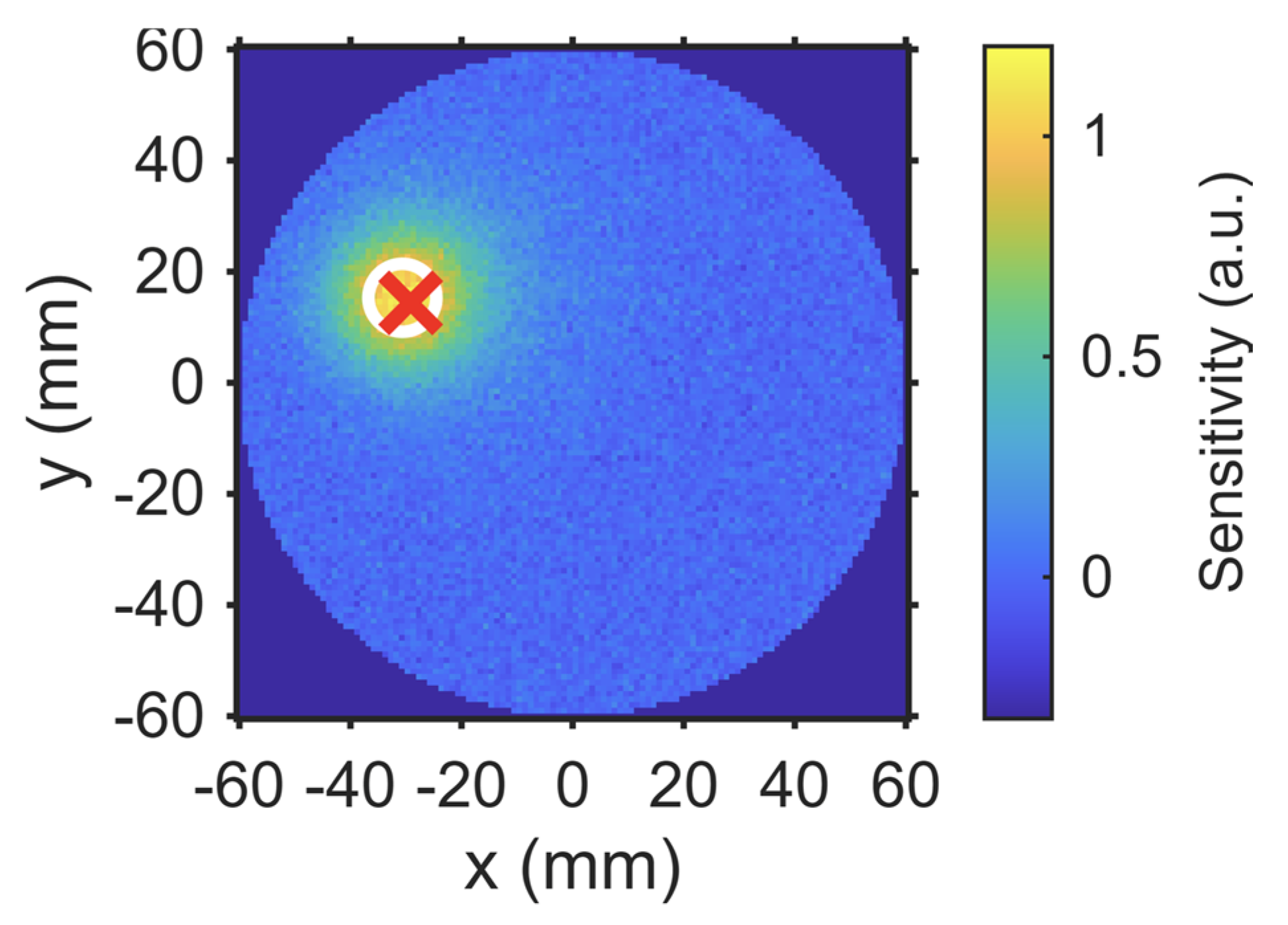
The analytical benchmark generated structured variation in antenna distance, ring offset, frequency coverage, channel family, tissue organisation and lesion-like conditions. The analytical localisation-error label was generated directly from the endpoint equation defined in Section 2.3 and Appendix A. Figure 2 presents a separately generated illustrative localisation-sensitivity map and did not determine the analytical label, candidate ranking or FDTD-transfer results.

3.2. Random Forest Provided the Lowest-Regret Analytical Shortlist

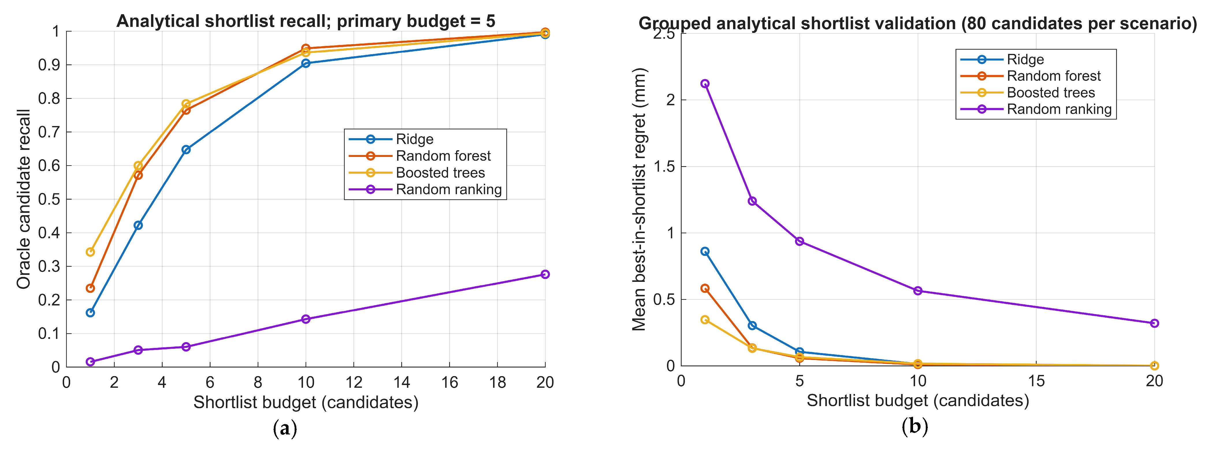
Analytical shortlisting was evaluated using grouped five-fold cross-validation repeated three times. At the prespecified primary budget of $K=5$, random forest achieved the lowest mean best-in-shortlist regret and was selected according to the frozen regret-first rule. Its mean and median regrets were 0.0575 and 0 mm, respectively, and every analytical validation scenario retained a candidate with regret no greater than 2 mm. Oracle recall was 0.7651, mean top-five overlap was 0.4011 and mean Spearman association was 0.7767. Boosted trees achieved higher oracle recall, top-five overlap and rank association than random forest, but their mean regret was slightly higher at 0.0661 mm.

Ridge regression produced a mean regret of 0.1057 mm, whereas random ranking performed substantially worse, with a mean regret of 0.9372 mm and near-zero rank association. These results indicate strong within-generator shortlist utility while showing that the evaluated ranking metrics did not identify the same preferred model.

The grouped analytical model performance at $K=5$ is summarised in

Table 3. Grouped analytical model performance at $K=5$.

Model	Mean Regret (mm)	Oracle Recall	Top-Five Overlap	Spearman Association	Fraction with Regret ≤2 mm
Ridge regression	0.1057	0.6476	0.2571	0.6830	1.0000
Random forest, frozen	0.0575	0.7651	0.4011	0.7767	1.0000
Boosted trees	0.0661	0.7841	0.4868	0.8367	1.0000
Random ranking	0.9372	0.0603	0.0381	−0.0095	0.9556

Model selection followed the frozen sequential hierarchy of lowest mean regret, followed, only where required, by highest oracle recall and highest top-five overlap.

. The scenario-conditioned ranking was additionally compared with the two candidate templates whose parameter definitions were identical across all scenarios. At $K=1$, random forest produced a mean regret of 0.5835 mm, compared with 0.8526 mm for the common 10 mm stand-off template and 0.9557 mm for the common 15 mm stand-off template. Both templates used the full 3–8 GHz band and full multistatic acquisition. The corresponding mean-regret reductions were 0.2691 mm (scenario-cluster 95% CI: 0.1436–0.3953 mm) and 0.3722 mm (95% CI: 0.2381–0.5018 mm), respectively. These results support an advantage of scenario-conditioned shortlisting within the analytical benchmark but do not establish superiority under FDTD, finite-antenna, hardware or clinical conditions.

The analytical advantage of model-guided ranking was maintained across the evaluated candidate budgets. Increasing $K$ improved oracle inclusion and reduced best-in-shortlist regret for all trained models, while random ranking remained consistently weaker. The budget-dependent oracle recall and best-in-shortlist regret are shown in Figure 3. The $K=5$ budget was retained for external evaluation because it imposed a restrictive candidate limit while preserving strong analytical-domain performance.

The 20-run fixed-partition model-seed analysis supported the stability of the regret-first selection. Across model-initialisation seeds, random forest achieved a mean regret of 0.0517 mm, with a standard deviation of 0.0049 mm and a range of 0.0418–0.0608 mm. Its mean oracle recall, top-five overlap and Spearman association were 0.775, 0.501 and 0.773, respectively. Random forest achieved lower mean regret than boosted trees in 16 of the 20 seed runs. The mean paired random-forest-minus-boosted-tree regret difference was $-0.0044$ mm, although the scenario-cluster 95% interval of $-0.0325$ to 0.0218 mm included zero. The model-seed analysis therefore showed that the selection of random forest was not an artefact of a single initialisation seed, but it did not establish statistically definitive or universal superiority over boosted trees.

3.3. Analytical Ranking Depended Primarily on Frequency and Channel Descriptors

Grouped permutation and leave-one-feature-group-out analyses were used to identify the descriptor groups supporting analytical-domain shortlisting. Frequency design produced the largest effect: permuting this group increased mean five-candidate regret by 0.2687 mm, with a scenario-bootstrap 95% interval of 0.1517–0.4199 mm, while removing the group and retraining the model increased regret by 0.2390 mm. Channel family produced the second-largest effects, with permutation and leave-one-feature-group-out regret increases of 0.1555 and 0.1436 mm, respectively.

Candidate geometry produced smaller but consistently positive effects. By contrast, the permutation intervals for tissue organisation, background conductivity and background dielectric properties spanned zero, and their leave-one-feature-group-out effects were negligible or negative on the prespecified split. These results quantify surrogate dependence within the analytical generator and do not establish that descriptor groups with small analytical effects are physically unimportant under FDTD, finite-antenna or experimental conditions.

On the corresponding grouped comparison split, the 21-descriptor target-agnostic model achieved a mean regret of 0.0856 mm, whereas the 26-descriptor oracle-assisted model achieved a mean regret of 0 mm. Access to privileged lesion and complete-scenario information therefore substantially simplified the analytical ranking task. Because this information would not ordinarily be available during prospective candidate selection, the oracle-assisted result was treated as a methodological upper bound rather than as deployable shortlisting performance. The grouped permutation and leave-one-feature-group-out results are summarised in

Table 4. Grouped permutation and leave-one-feature-group-out effects at $K=5$.

Feature Group	Permutation ($∆$) Regret (mm)	95% Interval (mm)	LOFO ($∆$) Regret (mm)
Frequency design	0.2687	0.1517 to 0.4199	0.2390
Channel family	0.1555	0.0906 to 0.2514	0.1436
Candidate geometry	0.1084	0.0235 to 0.2157	0.0446
Tissue organisation	0.0098	−0.0313 to 0.0365	−0.0054
Background conductivity	−0.0011	−0.0463 to 0.0329	−0.0381
Background dielectric properties	−0.0092	−0.0398 to 0.0049	−0.0136

Positive values indicate increased regret after permutation or feature-group removal. Negative leave-one-feature-group-out estimates indicate no evidence of positive dependence on that group in this split and should not be interpreted as beneficial physical effects.

.

3.4. The Operational FDTD Grid Preserved Shortlist-Level Decisions

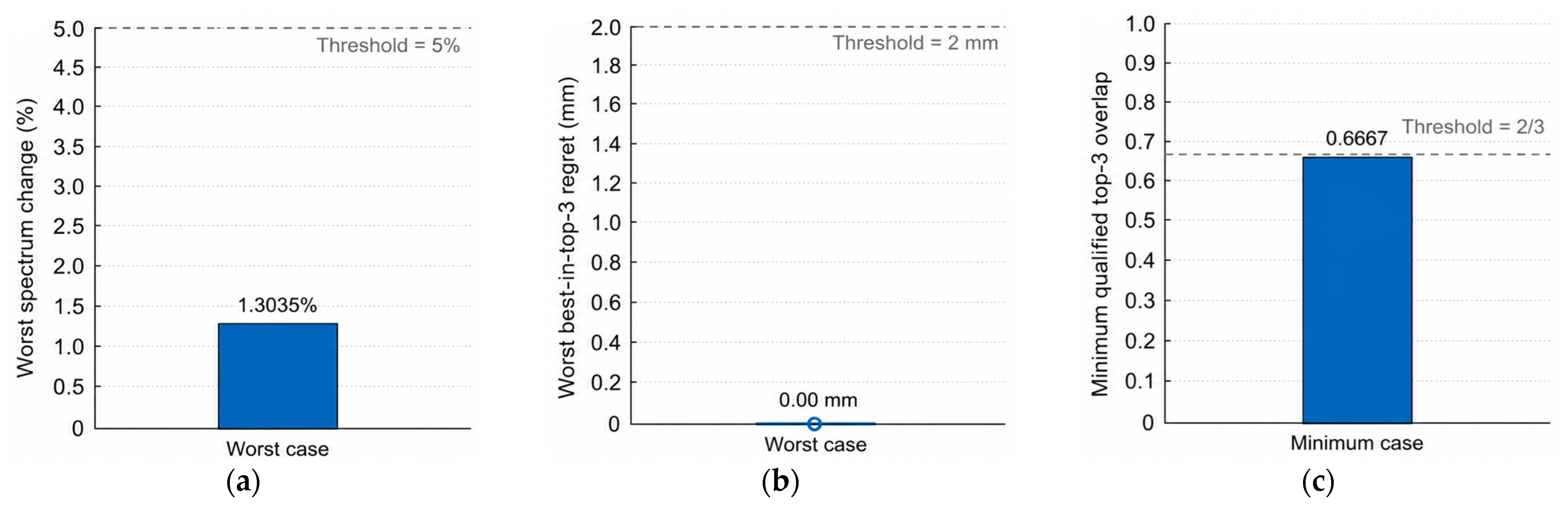
The numerical-reference assessment compared the 0.200 mm operational grid with the finer 0.180 mm grid across three scenarios at both stand-offs, yielding six scenario–stand-off units. All six met the prespecified shortlist-level criteria. At the reference shortlist size $K_{\mathrm{r}\mathrm{e}\mathrm{f}}=3$, the maximum candidate-used response-spectrum change was 1.3035%, below the 5% criterion. The maximum best-in-qualified-shortlist regret on the finer grid was 0 mm, indicating that every operational-grid shortlist retained at least one candidate attaining the qualified finite-library optimum on the finer grid. The minimum qualified top-three overlap was 0.6667, meeting the required value of $2/3$.

Candidate availability, tissue-map consistency, canonical propagation controls, convolutional perfectly matched layer checks, CPU–GPU agreement and candidate accounting also satisfied their respective criteria. The 0.200 mm grid was therefore retained for the held-out shortlist evaluation. Exact top-one identity was less stable: raw top-one identity was not preserved, and the maximum displacement of the reconstructed maximum was 2.3384 mm. These secondary sensitivity results indicate that the assessment supported shortlist-level decisions rather than numerical identity or exact preservation of a single nominal optimum.

Complete results are reported in Table A3. The three primary shortlist-level numerical-reference endpoints are summarised in Figure 4.

3.5. Candidate-Support Mismatch Defined the External Comparison

Exact candidate-support alignment was assessed before direct comparison of the analytical and FDTD outcomes. Only 12 of the 480 restricted FDTD scenario–candidate rows had one unique counterpart in the original analytical library within the same biological scenario; complete support alignment was therefore not achieved. Approximate and nearest-neighbour substitutions were not permitted because a direct matched analytical-to-FDTD comparison would otherwise have combined changes in electromagnetic representation with differences in candidate design. The external analysis consequently applied the frozen surrogate to the restricted FDTD candidate pool and compared its predicted ordering with the realised FDTD outcomes over the same pool. Given the incomplete alignment between the analytical and FDTD candidate libraries, the external evaluation was formulated as a decision-level transfer assessment rather than a direct field-level fidelity comparison. It quantified the extent to which the prospectively frozen analytical shortlist retained value under the restricted FDTD representation. The complete candidate-support alignment assessment is reported in Table A3.

3.6. The Frozen Shortlist Retained Partial but Unreliable Value Under FDTD Evaluation

The frozen random forest was evaluated on 12 held-out biological scenarios at stand-offs of 15 and 20 mm, yielding 24 scenario–stand-off units. Each unit contained 20 restricted candidates, of which the first five ranked by the frozen surrogate formed the retained shortlist. Every unit retained at least one localisation-qualified shortlisted candidate, so penalised regret equalled observed best-in-shortlist regret throughout the held-out evaluation. At $K=5$, mean penalised regret was 3.2127 mm, with a scenario-cluster 95% bootstrap interval of 1.319–5.789 mm. Qualified oracle recall was 0.1667, qualified top-three overlap was 0.2222, qualified top-five overlap was 0.3250 and qualified Spearman association was $-0.1444$. Fourteen of the 24 units, or 58.3%, retained a qualified candidate within 2 mm of the finite-library FDTD optimum. These results were markedly weaker than the grouped analytical-domain findings: the negative mean rank association and low qualified-optimum inclusion indicated that the analytical ordering was not preserved reliably. Nevertheless, the shortlist retained a near-optimal qualified candidate in more than half of the evaluation units. The surrogate therefore retained partial shortlisting value, but the evidence did not support its use as a dependable FDTD optimiser or as a replacement for evaluation of the complete restricted candidate library. The overall and stand-off-stratified held-out transfer results are summarised in

Table 5. Held-out same-support surrogate-to-FDTD transfer at $K=5.$

Endpoint	Overall, 24 Units	15 mm, 12 Units	20 mm, 12 Units
Mean penalised regret, mm (95% CI)	3.2127 (1.319–5.789)	4.8796 (1.729–9.468)	1.5458 (0.497–2.965)
Qualified oracle recall	0.1667	0.1667	0.1667
Qualified top-three overlap	0.2222	0.2500	0.1944
Qualified top-five overlap	0.3250	0.3500	0.3000
Qualified Spearman association	−0.1444	−0.1418	−0.1470
Fraction with regret $\le$2 mm	0.5833	0.4167	0.7500
Ambiguous fraction among selected candidates	0.3083	0.3833	0.2333

Stand-off strata are descriptive. Scenario-cluster resampling retained both stand-offs associated with each biological scenario.

.

Complete candidate identities, localisation errors, regret values, ranking agreement and ambiguity diagnostics for the 24 scenario–stand-off units are provided in

Table A4. Complete held-out surrogate-to-FDTD transfer results for the 24 scenario–stand-off units at $K=5.$ (A) Candidate-selection and regret outcomes. (B) Ranking agreement and ambiguity diagnostics.

(A)
Scenario	Stand-Off (mm)	Qualified FDTD Oracle Candidate ID	Oracle Error (mm)	Best Qualified Candidate in (K = 5)	Shortlist Error (mm)	Penalised Regret (mm)	Oracle Captured	Regret ≤ 2 mm
5	15	8	20.4765	19	25.9350	5.4585	No	No
5	20	26	26.9568	39	28.5243	1.5675	No	Yes
20	15	16	11.0485	16	11.0485	0.0000	Yes	Yes
20	20	37	25.2363	36	25.3421	0.1057	No	Yes
40	15	10	11.8082	19	13.7232	1.9150	No	Yes
40	20	23	11.2186	30	11.2186	0.0000	No	Yes
42	15	7	6.3339	10	9.1545	2.8206	No	No
42	20	40	1.5417	40	1.5417	0.0000	Yes	Yes
51	15	9	7.8864	20	9.9879	2.1015	No	No
51	20	27	9.3009	39	17.4189	8.1180	No	No
67	15	7	3.6438	16	8.7313	5.0875	No	No
67	20	26	9.9733	30	12.6222	2.6490	No	No
82	15	17	7.4885	16	7.5053	0.0168	No	Yes
82	20	37	6.8681	36	6.9032	0.0351	No	Yes
89	15	4	18.4484	20	26.8933	8.4449	No	No
89	20	37	8.6731	36	9.0578	0.3847	No	Yes
104	15	6	18.0857	19	19.4038	1.3182	No	Yes
104	20	21	21.8629	39	23.3678	1.5050	No	Yes
111	15	1	15.8234	20	19.3787	3.5553	No	No
111	20	30	5.6418	30	5.6418	0.0000	Yes	Yes
115	15	16	2.3508	16	2.3508	0.0000	Yes	Yes
115	20	37	0.8176	36	1.7228	0.9052	No	Yes
118	15	8	4.1337	20	31.9709	27.8372	No	No
118	20	28	9.7698	36	13.0491	3.2794	No	No
(B)
Scenario	Stand-Off (mm)	Qualified Top-Three Overlap	Qualified Top-Five Overlap		Qualified Spearman Association		Ambiguous Candidates in (K = 5)	Qualified Candidates in (K = 5)
5	15	0.0000	0.2000		−0.5663		1	4
5	20	0.0000	0.4000		−0.0505		1	4
20	15	0.3333	0.2000		−0.1048		2	3
20	20	0.3333	0.2000		−0.2615		1	4
40	15	0.3333	0.6000		0.3423		2	3
40	20	0.0000	0.2000		0.0429		1	4
42	15	0.3333	0.6000		0.0536		2	3
42	20	0.3333	0.4000		0.1123		1	4
51	15	0.6667	0.4000		0.1592		1	4
51	20	0.0000	0.0000		−0.4821		1	4
67	15	0.0000	0.4000		−0.1466		2	3
67	20	0.3333	0.4000		0.0933		1	4
82	15	0.3333	0.4000		−0.3890		2	3
82	20	0.3333	0.2000		−0.4857		1	4
89	15	0.0000	0.2000		−0.3481		2	3
89	20	0.3333	0.4000		−0.0857		1	4
104	15	0.3333	0.4000		−0.1341		3	2
104	20	0.0000	0.2000		−0.2397		2	3
111	15	0.0000	0.2000		−0.2431		2	3
111	20	0.0000	0.6000		−0.0330		1	4
115	15	0.6667	0.4000		0.1393		2	3
115	20	0.3333	0.4000		−0.1036		1	4
118	15	0.0000	0.2000		−0.4643		2	3
118	20	0.3333	0.2000		−0.2703		2	3

Notes: The qualified FDTD oracle was the candidate with the lowest localisation error among the non-ambiguous candidates in each stand-off-specific library of 20 candidates. The best shortlisted candidate was the qualified candidate with the lowest localisation error among the five candidates retained by the prospectively fixed random forest. All 24 shortlists contained at least one qualified candidate; penalised regret therefore equalled the observed best-in-shortlist regret in every evaluation unit. Oracle capture refers to candidate identity, whereas regret reflects localisation error. Zero regret without oracle capture was possible when different candidates produced the same minimum error, as occurred for Scenario 40 at a stand-off of 20 mm. Stand-off-specific results are descriptive because the two stand-offs associated with each biological scenario constitute paired observations.

.

3.7. Transfer Failure Was Structured by Frequency and Channel Family

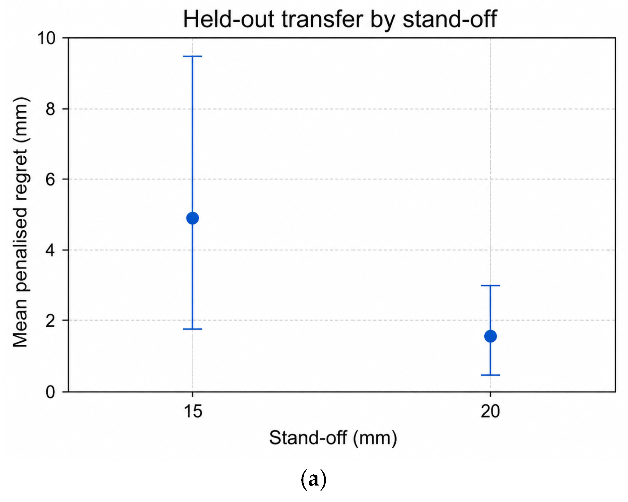
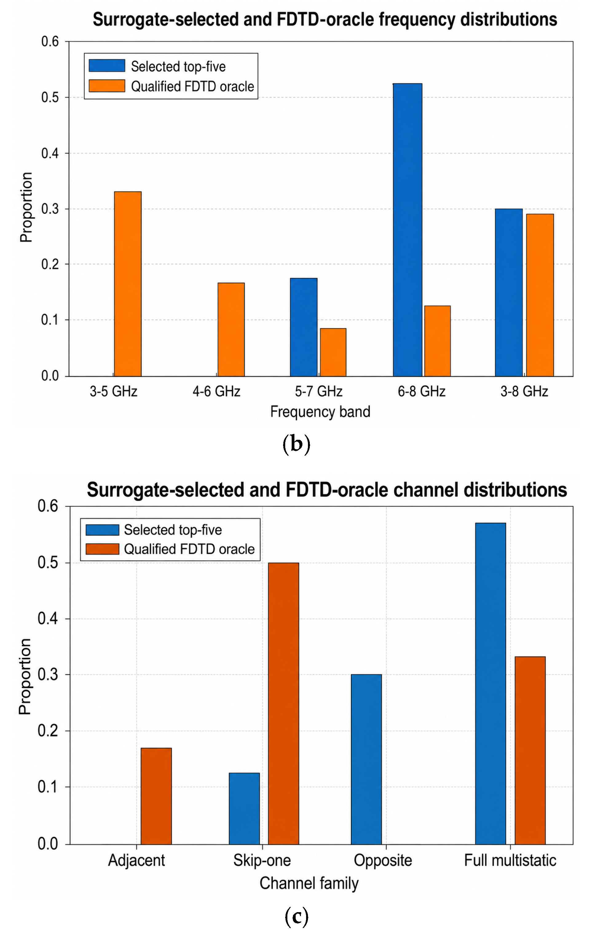
Transfer was descriptively more favourable at 20 mm than at 15 mm: mean penalised regret decreased from 4.8796 to 1.5458 mm, the proportion of units with regret no greater than 2 mm increased from 41.7% to 75.0%, and ambiguity expenditure decreased from 38.3% to 23.3%. However, the corresponding uncertainty intervals were wide and overlapping, so these differences do not establish a stand-off effect. The frequency composition of the surrogate shortlist also differed substantially from that of the qualified finite-library FDTD optima. Of the 120 selected top-five positions, 63, or 52.5%, used the 6–8 GHz band, whereas only three of the 24 qualified FDTD optima, or 12.5%, occurred in that band. No 3–5 or 4–6 GHz candidate appeared among the surrogate-selected positions, although these two bands supplied 12 of the 24 qualified FDTD optima. Channel-family preferences showed a similar mismatch. Full-multistatic candidates accounted for 69 of the 120 selected positions and eight of the 24 qualified FDTD optima. Opposite-channel candidates occupied 36 selected positions, or 30.0%, but supplied no qualified FDTD optimum. By contrast, skip-one candidates occupied only 15 selected positions, or 12.5%, but supplied 12 of the 24 qualified optima, while adjacent candidates were absent from the selected top-five positions but supplied four qualified optima. Localisation ambiguity was also strongly channel dependent.

Under the frozen ambiguity rule, the pre-held-out analytical evidence yielded ambiguity fractions of 5.3%, 19.3%, 98.7% and 3.3% for adjacent, skip-one, opposite and full in-plane multistatic candidates, respectively. The held-out FDTD library showed the same principal pattern, with corresponding fractions of 9.2%, 6.7%, 95.8% and 3.3%. The transfer gap was therefore concentrated on candidate dimensions that strongly influenced analytical selection rather than appearing solely as a uniform increase in localisation error. In particular, the surrogate allocated a substantial proportion of its shortlist to upper-frequency and opposite-channel candidates, whereas the qualified FDTD optima were distributed more broadly across frequency bands and were more frequently associated with skip-one channels. These comparisons remain descriptive because only 12 independent biological scenarios were evaluated, and the five selected positions within each scenario–stand-off unit were nested observations. Figure 5 summarises the stand-off-specific regret and the mismatch between surrogate-selected and FDTD-optimal frequency bands and channel families.

3.8. Shortlisting Reduced Candidate-Level Assessment but Not FDTD Propagation

The complete held-out restricted library contained 480 candidate evaluations, of which the $K=5$ policy retained 120, corresponding to a 75% reduction and a fourfold decrease in candidate-level reconstruction or configuration assessment. Candidate-level channel–frequency samples decreased from 1,036,800 to 548,496, representing a 47.1% reduction in this workload proxy. This reduction did not produce a fourfold decrease in FDTD propagation because the 20 candidates within each scenario–stand-off unit reused common broadband field responses. The held-out campaign therefore comprised 24 unique scenario–stand-off broadband configurations, each evaluated using 16 transmitter positions and two biological states, yielding $768$ transmitter-state FDTD runs. All 768 recorded quality-control rows used GPU execution and met the frozen numerical criteria. The computational benefit therefore concerned candidate-level reconstruction, configuration comparison and channel–frequency processing rather than the number of Maxwell field solutions. A reliable total FDTD wall-clock time was unavailable in the preserved execution records and was not reconstructed retrospectively. Accordingly, the fourfold reduction in candidate-level assessment should not be interpreted as a fourfold FDTD speed-up.

4. Discussion

The analytical benchmark showed that the finite antenna–frequency–channel design space could be shortlisted reproducibly within the controlled generator. Comparison with the two common fixed templates further supported scenario-conditioned shortlisting within this analytical setting. However, the held-out FDTD findings showed that this analytical-domain advantage was not representation-independent. The surrogate therefore learned the preference structure encoded by the analytical model rather than a universally preserved electromagnetic ordering. Its retained value was partial rather than negligible: the frozen shortlist frequently included a candidate close to the restricted FDTD optimum, but low optimum inclusion, limited shortlist agreement and negative rank association did not support its use for final configuration selection. The surrogate should therefore be used for provisional candidate prioritisation followed by independent electromagnetic evaluation.

The transfer gap was concentrated in the candidate dimensions that most strongly influenced analytical ranking. The surrogate favoured upper-frequency and opposite-channel configurations, whereas the qualified FDTD optima were distributed more broadly across frequency bands and occurred more often among skip-one candidates. Opposite-channel configurations were also frequently localisation-ambiguous and did not supply a qualified FDTD optimum. Analytical feature importance should therefore not be interpreted directly as a transferable design rule; instead, highly influential frequency, channel and geometry descriptors identify the dimensions requiring the most stringent external validation. Performance was descriptively better at 20 mm than at 15 mm, but the small paired scenario set and overlapping uncertainty intervals do not establish a stand-off effect.

The principal contribution is a validation-aware decision framework rather than a new surrogate algorithm. The framework separates grouped analytical development from a frozen external challenge, evaluates whether the operational numerical grid preserves shortlist-level decisions, retains localisation ambiguity in the analysis and assesses support alignment between the analytical and FDTD candidate libraries. Because exact candidate correspondence was incomplete, the observed transfer gap cannot be attributed solely to differences between the analytical and FDTD forward models. This support-aware interpretation prevents combined changes in candidate design and electromagnetic representation from being presented as a pure solver comparison. It also shows that descriptor-based modelling, even when physically motivated, does not remove the need for independent evaluation under the representation relevant to the intended design claim.

The frozen shortlist reduced candidate-level reconstruction and configuration assessment, supporting its use as an initial shortlisting mechanism when downstream evaluation is costly. This saving should not be equated with an equivalent reduction in electromagnetic propagation because multiple candidates reused the same broadband field responses. The practical computational benefit therefore depends on whether the dominant cost arises from field generation, reconstruction, channel–frequency processing, configuration comparison or experimental acquisition. The concentration of selected candidates within particular frequency bands and channel families also suggests that future shortlist policies may benefit from prespecified diversity constraints rather than relying exclusively on predicted rank; any such policy should be defined prospectively and evaluated on new held-out scenarios. Operationally, the framework provides a gated design pathway: construct the analytical candidate library, develop the surrogate using grouped scenarios, freeze the model and shortlist budget, qualify the independent numerical representation and evaluate the retained candidates before final selection. Failure to preserve ranking at the external gate does not eliminate the surrogate’s value for preliminary shortlisting, but it prevents the analytical shortlist from being promoted directly to a final electromagnetic configuration.

No experimental study was performed. The conclusions are restricted to a controlled analytical benchmark and a restricted 2-D ${\mathrm{T}\mathrm{M}}_z$ FDTD challenge using ideal in-plane sources and receivers. The model omitted finite antennas, feeds, ports, loaded radiation patterns, mutual coupling, out-of-plane propagation, calibration effects and measurement noise.

Only 12 independent held-out biological scenarios and two stand-offs were evaluated, and the finer numerical grid served as a comparator rather than exact electromagnetic truth. In addition, incomplete candidate-support alignment prevented separation of electromagnetic-model shift from candidate-library shift. Future studies should use a prospectively frozen candidate manifest shared exactly across analytical and higher-fidelity representations, followed by three-dimensional finite-antenna simulation, tissue-loaded phantom measurements and hardware testing incorporating coupling, positioning, calibration, noise and repeatability. Within the present scope, the surrogate should be used to generate an auditable shortlist for subsequent validation rather than to determine the final antenna, frequency or channel configuration.

5. Conclusions

This study developed a surrogate-ranking framework for finite-budget broadband antenna, frequency and channel selection and assessed whether its analytical-domain candidate preferences transferred to a separately implemented restricted 2-D ${\mathrm{T}\mathrm{M}}_z$ FDTD representation. Although the frozen surrogate achieved strong and reproducible shortlisting performance within the controlled analytical generator, its candidate ordering did not transfer reliably in the held-out FDTD challenge. The shortlist retained partial shortlisting value by preserving a qualified candidate within 2 mm of the finite-library FDTD optimum in more than half of the evaluated scenario–stand-off units. However, low optimum inclusion, limited shortlist agreement and negative rank association did not support its use as a final FDTD optimiser. The principal contribution is therefore a validation-aware workflow in which analytical surrogates generate provisional, auditable candidate shortlists for subsequent independent electromagnetic evaluation. The approach reduced candidate-level reconstruction and configuration assessment but did not produce an equivalent reduction in electromagnetic-field propagation because multiple candidates reused common broadband responses. Three-dimensional finite-antenna simulation, phantom measurements and hardware validation remain necessary before broader system-performance claims can be made.