


Abstract
This study proposes an intelligent speed-loop controller for a brushless DC motor (BLDCM) drive implemented under a field-oriented control (FOC) scheme. The controller is constructed by embedding the coati optimization algorithm (COA) into a composite sliding mode theory (CSMT) control structure. In sliding mode control (SMC), the use of only one reaching law normally produces a design trade off: increasing the reaching speed tends to aggravate overshoot or chattering, whereas reducing switching activity often slows convergence. To mitigate this compromise, the proposed controller adopts a composite reaching law (CRL) formed by an exponential component and a power component. When the system trajectory is distant from the sliding surface, the exponential component strengthens the reaching action and shortens the transient interval. When the trajectory moves close to the sliding surface, the power component decreases the effective switching intensity, thereby attenuating high-frequency chattering and reducing the overshoot associated with an aggressive exponential action. For adaptive gain selection, the COA search variables are chosen as four controller parameters: the sliding mode gain, the exponential reaching gain, the power reaching gain, and the power exponent. The fitness index is established from the rotor-speed tracking error and the time variation in that error. By imitating the hunting and predator-avoidance behaviors of coatis, the optimization process updates candidate solutions and selects the parameter combination that best matches the current operating condition. The resulting gains are supplied to the composite sliding mode controller (CSMC) so that the BLDCM can follow speed commands rapidly while preserving stable regulation. Because the proposed method performs online optimization of controller gains rather than data-driven training, it can be realized without a large training dataset. MATLAB/Simulink simulations are carried out to examine the effectiveness of the proposed strategy. The controller is compared with four benchmark methods, namely power reaching law (PRL)-based SMC, exponential reaching law (ERL)-based SMC, non-optimized composite reaching law SMC, and zebra optimization algorithm (ZOA)-assisted ERL-based SMC. The simulation results demonstrate that the proposed COA-based composite sliding mode controller improves both speed command-tracking and load-disturbance rejection relative to the comparative controllers.
1. Introduction
Brushless DC motors (BLDCMs) [1,2] due to their superior characteristics of high torque output, high power density, compact size, and low maintenance costs, have found broad application across various industries, including industrial automation, electric vehicles, aerospace technology, and precision robotic arms. However, as modern industry imposes increasingly stringent requirements on dynamic response speed and steady-state position control accuracy, conventional control methods have become inadequate for meeting the demands of high-performance servo drive systems. Consequently, field-oriented control (FOC) technology [3] integrated with intelligent controllers is predominantly adopted in industrial applications. Conventional FOC achieves closed-loop system control through coordinate transformation and three proportional-integral (P-I) controllers [4]: the speed controller, the q-axis current controller, and the d-axis current controller, thereby enabling linear control characteristics for the BLDCM. Nevertheless, although conventional P-I controllers are comparatively simple to implement, they frequently exhibit sluggish system response and excessive tracking errors when confronted with rapidly varying speed commands or load disturbances, resulting in degraded overall control performance and accuracy.
To improve robustness, several nonlinear and intelligent control techniques have been developed; however, each approach still has practical limitations. Among them, the sliding mode controller (SMC) [5] is attractive for nonlinear systems because of its strong disturbance-rejection capability. Frequently used reaching laws include the constant speed reaching law (CSRL), the exponential reaching law (ERL), and the power reaching law (PRL). When a single reaching law is used alone, the controller generally cannot satisfy fast command tracking and strong load regulation at the same time. The CSRL has a simple form, but because it lacks integral compensation, the tracking process may become prolonged. The ERL can reduce the convergence time, but it may cause severe overshoot in the speed response. The PRL is effective in mitigating chattering and over-shoot near the sliding surface; however, the resulting control effort can be insufficient when external disturbances are applied. Other adaptive techniques also present restrictions. Extension theory (ET) [6] can adjust controller parameters flexibly for different operating requirements, but the system may become unstable if the operating point leaves the predefined neighborhood domain. The zebra optimization algorithm (ZOA) [7] is simple and has a certain ability to avoid local optima, yet its search performance becomes less effective when the number of tuning parameters increases.
To overcome the aforementioned shortcomings of existing controllers and to enhance overall control performance, it is necessary to combine different methodologies to achieve adaptive capability. Representative examples include the combination of ET with a P-I controller [8] and the combination of the ZOA with an exponential reaching law-based sliding mode controller (ERLSMC) [9]. Nevertheless, although ET combined with a P-I controller can successfully yield superior controller parameters, parameter tuning depends on an approximation-based approach using look-up tables, which tends to produce inaccurate results when the available data is limited. As for the ZOA combined with the ERLSMC, while it successfully suppresses the overshoot of the standalone ERLSMC and demonstrates superior overall performance, the use of the ERL inherently prevents the controller from simultaneously achieving rapid convergence and effective chattering suppression. Consequently, as the system approaches a steady state, a portion of the convergence speed must be sacrificed in exchange for enhanced stability. Furthermore, under load disturbances, insufficient gain may cause a relatively large dynamic speed error, thereby prolonging the settling time required for the system to recover to a steady state.
In response to these issues, this paper develops a speed-control method that combines the coati optimization algorithm (COA) [10] with composite sliding mode theory (CSMT). In the proposed scheme, the BLDCM drive performs adaptive speed regulation over the rated operating range by automatically tuning four essential gains of the composite sliding-mode controller. The purpose of this design is to improve the transient speed response while maintaining high steady-state accuracy for the BLDCM drive system.
2. BLDCM Motor Drive System
A BLDCM is composed of a three-phase stator winding and a rotor carrying high-flux-density permanent magnets. Unlike a brushed DC motor, it does not use mechanical brushes or a commutator; instead, phase commutation is achieved electronically. For accurate control, the drive requires precise rotor-position information. While traditionally acquired from physical devices such as Hall sensors or optical encoders, this information can also be estimated using speed-sensorless techniques. In this study, the rotor-position information required for FOC is obtained through a speed-sensorless estimation scheme rather than mechanical position sensors. This position information provides the phase reference required for FOC and keeps the stator and rotor fluxes orthogonal, which is essential for high-performance speed regulation.
2.1. Dynamic Equations of FOC for the BLDCM
FOC, also known as vector control, is used to reduce the modeling complexity of the BLDCM drive. Through coordinate transformation [11], the voltage and flux-linkage relations that are originally described in the three-phase stationary frame are transformed into a two-axis synchronously rotating frame. After this transformation, the motor model can be expressed in a form that is more convenient for control analysis and controller synthesis [12].
In the synchronously rotating d-q reference frame, the BLDCM is modeled under the assumptions that the rotor has no damper winding and that the permanent magnets are mounted on the rotor surface. Under these conditions, the magnetic excitation generated by the permanent magnets can be represented by an equivalent constant excitation source. Accordingly, the rotor excitation current is treated as a constant, i.e., . When the angular velocity of the selected two-axis reference frame is set equal to the rotor angular velocity, i.e., , the reference frame rotates synchronously with the rotor. For a synchronous motor, the electrical rotor angular velocity is identical to the synchronous angular velocity; hence, . Because the permanent-magnet flux is aligned with the d-axis, it can be modeled as an equivalent constant d-axis current source , whereas the q-axis rotor current component is zero. Therefore, the stator flux linkages are obtained as Equations (1) and (2).
where and denote the stator flux linkages on the d-axis and q-axis, respectively, and is the permanent-magnet flux linkage in the stator winding. Using these flux-linkage expressions, the stator voltage equations are written as Equations (3) and (4).
where and are the d-axis and q-axis stator voltages, respectively; is the stator resistance; and represent the d-axis and q-axis stator currents, respectively; is the electrical angular velocity; and are the stator inductances along the d-axis and q-axis, respectively. Since the d-axis is aligned with the stator windings, whereas the q-axis is aligned with the stator core, the magnetic reluctance along the q-axis exceeds that along the d-axis. Furthermore, according to , the inductance is inversely proportional to the magnetic reluctance. Hence, . The electromagnetic torque equation and the mechanical dynamic equation of the BLDCM can be expressed as Equations (5) and (6), respectively.
where denotes the electromagnetic torque; is the number of poles; represents the moment of inertia; is the mechanical rotational speed; is the load torque; and B denotes the viscous friction coefficient.
Under the FOC framework, the d-axis stator current is controlled to be zero, i.e., . Therefore, the voltage equations and torque equation given in Equations (3)–(5) can be reduced to Equations (7)–(9), respectively.
According to Equation (9), the electromagnetic torque is proportional to the q-axis stator current. Hence, the torque constant can be defined as Equation (10).
Substituting Equation (10) into the BLDCM mechanical motion equation yields the rearranged form shown in Equation (11).
2.2. Decoupling Control and Speed Sensorless FOC Architecture of the BLDCM
In a conventional FOC scheme, the drive is generally implemented as a two-loop control structure that consists of an external speed loop and an internal current loop. The speed loop calculates the speed error and generates the current command for the current loop. This command is compared with the feedback current obtained after coordinate transformation, and the current error is then regulated by the P-I controller in the current loop. The regulated signal is further transformed to synthesize the required voltage vector. After the voltage vector is generated, space vector pulse-width modulation (SVPWM) produces the switching signals for the six inverter power devices [13]. Through this procedure, the motor can track the commanded speed and the steady-state error can be significantly reduced. Because this study adopts a speed sensorless direct FOC configuration, a sliding mode theory (SMT)-based speed estimator [14] is employed to estimate the instantaneous rotor speed and position, thereby replacing the mechanical position sensor.
In the current loop, the stator current is decomposed into two orthogonal components: the flux-producing component and the torque-producing component. This decomposition enables the AC motor to exhibit control characteristics similar to those of a separately excited DC motor. However, Equations (3) and (4) show that nonlinear coupling terms remain in the BLDCM voltage equations, and these terms may deteriorate current-loop performance. Therefore, decoupling control [15] is introduced as a compensation method to remove the coupling effect and to improve the linearity of the current-loop dynamics. According to the feedback-control principle, the d-axis current error is processed by the P-I regulator, and the resulting output is expressed as Equation (12).
The output signal is combined with the d-axis current-loop response and is then converted through coordinate transformation to generate the three-phase voltage command supplied to the inverter. To ensure linear control characteristics in the current loop, a suitable compensation term must be added before the coordinate transformation. Accordingly, the d-axis voltage command is defined in Equation (13).
Substituting Equation (13) into the d-axis voltage equation in Equation (3) yields the decoupled d-axis current dynamic equation, as given in Equation (14).
In the same manner, the q-axis current-loop output and its corresponding voltage command are formulated as Equations (15) and (16), respectively.
Substituting Equation (16) into the q-axis voltage equation in Equation (4) yields the decoupled q-axis current dynamic equation, as expressed in Equation (17).
It should be noted that the feedforward decoupling terms in Equations (13) and (16) are calculated using nominal motor parameters. In practical operation, variations in , , and may cause residual coupling and current tracking errors. These effects are mainly handled by the inner P-I current controllers and may appear as equivalent uncertainties or disturbances in the outer speed loop. Therefore, the proposed COA-CSMC focuses on improving the robustness of the speed-loop response against such equivalent disturbances.
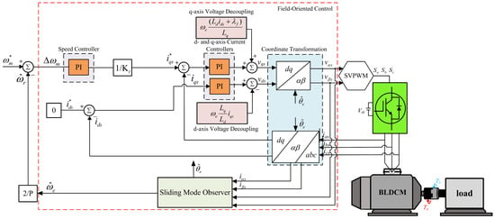
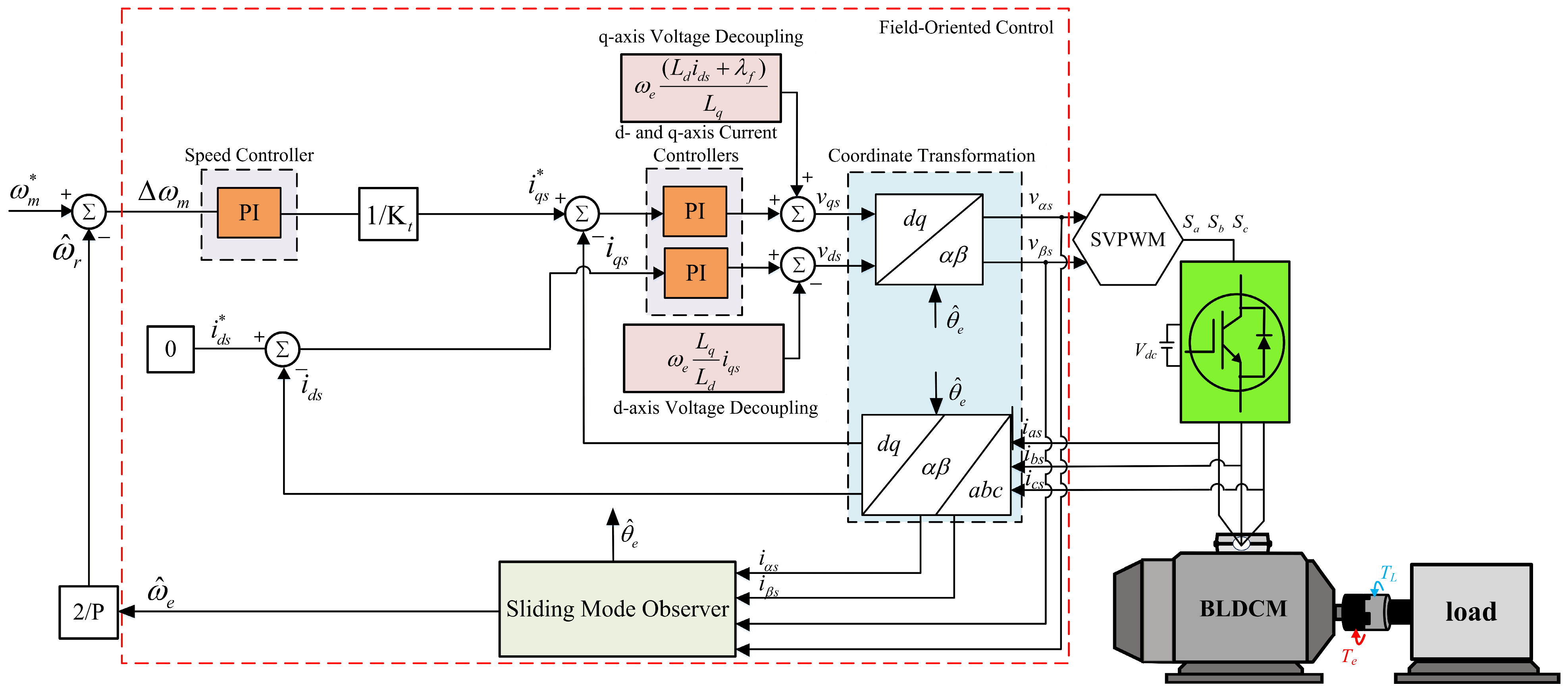
By integrating the aforementioned speed sensorless speed estimation scheme and decoupling compensation strategy, the complete architecture of the speed sensorless FOC BLDCM drive system can be constructed, as illustrated in Figure 1.
Figure 1.
Block diagram of the conventional speed sensorless FOC architecture for the BLDCM drive system.
3. Proposed Speed Controller Incorporating an Intelligent Optimization Algorithm
Within the conventional FOC framework of BLDCM drive systems, the speed-loop controller is predominantly realized by means of a P-I controller. Nevertheless, a conventional P-I controller inherently struggles to concurrently attain adequate speed command tracking accuracy and satisfactory load regulation performance. To address this limitation and enhance the dynamic response as well as the disturbance rejection capability of the BLDCM speed regulator, this work develops a novel intelligent controller intended to supersede the conventional P-I controller within the speed control loop. The proposed control framework employs the COA to determine the suitable gain settings for the composite sliding mode controller (CSMC). During the optimization procedure, each candidate parameter set is evaluated according to the rotor speed tracking error and the variation rate of this error, which are used together to construct the fitness index of the COA. After the search process is completed, the best parameter combination obtained by the COA is assigned to the CSMC. Through this mechanism, the speed controller can adjust its gains according to different operating conditions, thereby improving the speed regulation performance of the BLDCM drive system.
3.1. Composite Sliding Mode Controller (CSMC)
The BLDCM drive system exhibits nonlinear coupling and is easily affected by parameter variations and load disturbances. For this reason, variable structure control is considered suitable for enhancing the robustness of the speed loop [16]. In SMC, the reaching law directly influences the transient response, disturbance rejection capability, and chattering behavior. The CSRL has a simple structure, but its fixed reaching rate makes it difficult to simultaneously achieve fast convergence and low chattering. The ERL improves the reaching speed when the system state is far from the sliding surface, whereas an excessive exponential gain may lead to overshoot. In contrast, the PRL can reduce the switching intensity near the sliding surface, but its control effort may be insufficient when a large load disturbance occurs. To balance these characteristics, this study adopts a CSMC based on the variable structure control concept reported in [17] and the improved power exponential reaching law (PERL) applied in [18]. The adopted controller combines an exponential term and a power term so that rapid convergence can be maintained under large tracking errors while chattering can be suppressed near the sliding surface.
3.1.1. Design of the Composite Sliding Mode Controller
In the FOC structure, the d-axis current command is set to zero for speed loop design. Under the ideal operating assumption, the viscous friction term is neglected, the simplified mechanical equation of the BLDCM is expressed as Equation (18).
For speed tracking control, the state variables are defined by the speed error and the derivative of the speed error, as defined in Equation (19).
where represents the speed tracking error, and represents the variation rate of the speed error. Since the speed command is assumed to be constant during one control interval, differentiating the state variables and substituting the simplified mechanical model gives
The main objective of the SMC is to constrain the system state trajectory to move along the sliding surface. The sliding mode variable can be expressed in the form of Equation (21).
where denotes the sliding mode variable, c is the sliding mode control gain. When the system reaches , the state trajectory is constrained on the sliding surface, and the speed tracking error converges toward zero according to the designed sliding dynamics.
To drive the system trajectory toward the sliding surface, the reaching law must be properly selected. The CSRL, ERL, and PRL are commonly expressed as Equations (22)–(24), respectively.
- (1)
- CSRL:
- (2)
- ERL:
- (3)
- PRL:
Based on the mathematical properties of the above three reaching laws, their control effects can be summarized as follows. The CSRL is structurally simple because its reaching speed is governed by the fixed gain ; however, a small value of slows the motion toward the sliding surface, whereas an overly large value increases switching activity and may induce chattering. The ERL adds the term , which enlarges the reaching force when the system state is far from the sliding surface and therefore improves the transient response under large tracking errors or load disturbances. Nevertheless, an excessive exponential gain may lead to overshoot, while an insufficient gain weakens disturbance rejection. The PRL adjusts the reaching action according to the magnitude of the sliding variable. As the trajectory approaches the sliding surface, the power term decreases the effective switching action and helps suppress chattering; however, when the system state is far from the sliding surface, its reaching force may be lower than that of the exponential term, resulting in a slower response under large error conditions.
The above characteristics show that none of the single reaching laws can satisfy all performance requirements. Therefore, this paper adopts a composite reaching law (CRL) that combines the fast convergence of the ERL when the state is far from the sliding sur-face with the finite-time convergence and chattering-reduction properties of the PRL near the surface. The mathematical expression of the adopted CRL is given in Equation (25).
where denotes the exponential reaching gain, denotes the power reaching gain, and is the power exponent. When is large, the linear term dominates the reaching process and accelerates convergence. When the trajectory approaches the sliding surface, the power term becomes more influential, which helps reduce chattering while maintaining sufficient control effort.
Subsequently, by differentiating Equation (21), the sliding mode dynamics can be written as , where is the time derivative of the q-axis current. Combining this relation with Equation (25), the controller function u can be obtained as Equation (26).
Therefore, the q-axis reference current generated by the speed loop is obtained as Equation (27).
The obtained is subsequently provided to the inner current loop of the FOC system.
3.1.2. Stability Analysis
The stability of the adopted CSMC is examined using Lyapunov stability theory [19]. The Lyapunov candidate function is selected as Equation (28).
This candidate function is positive definite for and represents the deviation of the system trajectory from the sliding surface. According to the Lyapunov stability criterion, the time derivative of must satisfy when . Taking the time derivative of Equation (28) and substituting the adopted CRL yields Equation (29).
and thus
From Equation (30), since , and since both and are strictly greater than zero whenever the first term and the second term are both negative. This confirms that the Lyapunov stability condition is satisfied, thereby proving that the adopted CRL can render the system asymptotically stable.
Furthermore, the finite time convergence property can also be verified from the reaching law. For , the sign function can be removed during the reaching phase, and the reaching law becomes
From Equation (31), it can be observed that this equation is a nonlinear Bernoulli differential equation. To solve it using the general solution formula of a first-order linear differential equation, a variable transformation must first be performed. Therefore, an auxiliary variable is introduced and defined as Equation (32).
By differentiating Equation (32), Equation (33) can be obtained.
Substituting Equations (31) and (32) into Equation (33) and rearranging the result, the standard first-order linear differential equation can be obtained as Equation (34).
Applying the general solution formula to Equation (34) and (35) can be obtained
After rearrangement, Equation (36) can be obtained.
Let the initial condition be . By substituting Equation (32) into Equation (36), the constant C as shown in Equation (37).
Finally, by substituting Equation (37) back into Equation (36) and then converting the result according to Equation (32), the time-domain solution of the sliding mode variable scan be derived as Equation (38).
From Equation (38), it can be observed that the expression inside the brackets contains an exponential term that decays with time and a negative constant term. Therefore, when t reaches a certain time instant , the value inside the brackets becomes zero, i.e., , indicating that the system has completely reached the sliding surface. Finally, by setting and in Equation (38), the effective convergence time can be derived as Equation (39).
From Equation (39), it can be verified that the proposed CRL can ensure that the system converges to the sliding surface within a finite time . This characteristic is superior to the limitation of the conventional ERL, which can only achieve asymptotic convergence as .
3.2. Coati Optimization Algorithm
The COA is a novel swarm intelligence optimization algorithm proposed in 2023 by Mohammad Dehghani et al. [10]. The theoretical design of this algorithm is inspired by two distinct behavioral patterns observed in coatis within broad natural environments: namely, the foraging behavior exhibited during the hunting of green iguanas and the escape behavior adopted in response to predator threats. Through the aforementioned two behavioral mechanisms, the population can effectively determine which regions within the solution space offer more favorable survival resources, i.e., superior fitness values, and which regions are subject to lower predator threats. Accordingly, the population is guided to migrate toward the optimal survival location, which corresponds to the position of the global optimal solution.
3.2.1. Hunting Behavior
Coatis are diurnal mammals belonging to the family Procyonidae and are mainly distributed throughout the Americas. As omnivorous animals, their primary food sources include spiders, small birds, lizards, crocodile eggs, and bird eggs, among which green iguanas are one of the most preferred prey of coatis. Since green iguanas usually rest in trees and move rapidly, it is difficult for a single coati to capture them. Therefore, coatis exhibit a highly intelligent group hunting strategy. First, some coati members are responsible for climbing trees and intimidating the iguanas, forcing them to fall to the ground. The remaining members wait below the trees and immediately surround and attack the iguanas once they fall. Accordingly, in the algorithmic model, the position of the prey, namely the iguana, is defined as the current global optimal solution. This behavior corresponds to the global exploration phase of the algorithm. The initialization values of the algorithm are expressed as Equation (40).
where denotes the initial position of the i-th coati in the j-th dimension; and are the lower and upper bounds of the j-th search dimension, respectively; and is a random number within the range [0, 1].
This stage of the algorithm is divided into two groups. The first group is the tree-climbing group, which accounts for half of the total population, i.e., (N/2). Its position update strategy simulates the process by which coatis move toward the iguana in the tree. By continuously approaching the current optimal solution, this group explores potential regions within the solution space. The mathematical model of this behavior is expressed as Equation (41).
where denotes the updated new position of the i-th coati, is the current position, and represents the position of the prey in the j-th dimension. The parameter is randomly assigned as 1 or 2, which is introduced to simulate the uncertainty of coati movement, increase the randomness of the search path, and prevent the algorithm from premature convergence.
The second group is the ground-waiting group, which includes the remaining individuals, i.e., (N − N/2). When the iguana is frightened by the tree-climbing group and falls from the tree, its landing position is random. It is assumed that the iguana randomly falls to a certain position in the search space, denoted as . The ground-waiting coatis then evaluate this random landing position and determine their subsequent action. If the fitness value at the iguana landing position is better than that of the current coati, the coati moves toward that position. Otherwise, the coati randomly adjusts its position to search for other opportunities. The mathematical model of this decision mechanism is expressed as Equations (42) and (43).
where denotes the fitness value at the iguana landing position, and denotes the current fitness value of the i-th coati. From Equation (43), it can be observed that the ground-waiting group not only performs jump-type searches using the random iguana landing position , but also actively expands the search range under unfavorable conditions, thereby improving the ability of the algorithm to escape from local optima.
Finally, the algorithm adopts a greedy selection rule to determine whether the position should be updated. If the fitness value of the new position is better than the fitness value of the original position , the coati moves to the new position; otherwise, it remains at its original position. Whether the position is updated is expressed as Equation (44).
3.2.2. Behavior of Escaping from Predators
The second stage of the COA is the behavior of escaping from predators. This stage corresponds to the local exploitation phase of the algorithm and is formulated based on the escape response of coatis when encountering predator threats, such as jaguars and raptors. When a coati senses danger, it searches for the safest hiding place near its current position rather than moving blindly over a long distance.
To transform this behavior into a mathematical model with convergence capability, the algorithm introduces a local search region that dynamically shrinks as the number of iterations n increases. Its definition is given in Equation (45).
where n denotes the current number of iterations, and and are the original lower and upper bounds of the search space in the j-th dimension, respectively. From Equation (45), it can be observed that as the number of iterations increases, the local search radius decreases nonlinearly at a rate of 1/n. The physical meaning of this design is that when n is small in the early stage of the algorithm, the coati has a larger degree of movement freedom, which helps it escape from local optima. In contrast, when n becomes large in the later stage, the activity range of the coati is restricted to an extremely small neighborhood, forcing it to focus its search near the current best solution, thereby substantially improving the solution accuracy and convergence stability.
Based on the aforementioned local boundaries, the candidate position update formula for the coati during the second phase is updated according to Equation (46).
where is the candidate position of the coati during the predator-avoidance phase, is the current position, and is a random number within the range [0, 1]. The term in Equation (46) takes values within the interval [−1, 1], which imparts randomness to the search direction, thereby simulating the uncertain escape path of the coati during flight from predators.
Finally, the algorithm likewise adopts a greedy selection rule to determine whether the position should be updated. If the fitness value of the new position is better than the fitness value of the original position, the coati moves to the new position; otherwise, it retains its current position. Whether the position is updated is expressed as Equation (47).
3.3. Speed Control Based on the COA Combined with the CSMC
The present work employs an SMC constructed upon both power and exponential reaching laws to serve as the speed controller within the BLDCM drive system. Unlike the conventional ERLSMC, the proposed controller demonstrates a notable capability to eliminate speed overshoot while simultaneously enhancing the overall stability of the system dynamic response. Nevertheless, if the parameter tuning is not fully optimized, residual minor overshoot or chattering may still persist. In view of this, the controller requires the simultaneous adjustment of four gain parameters to achieve optimal control performance. The mutual interactions among these parameters are complex, making it difficult to obtain the optimal combination through conventional trial-and-error methods. Therefore, in this study, the COA is employed to define the ranges of the aforementioned four gain parameters as the upper and lower boundaries of the algorithm’s search space, respectively. Meanwhile, the speed error between the motor speed command and the actual speed, together with the rate of change in the speed error, is utilized as the feature for calculating the initial fitness value.
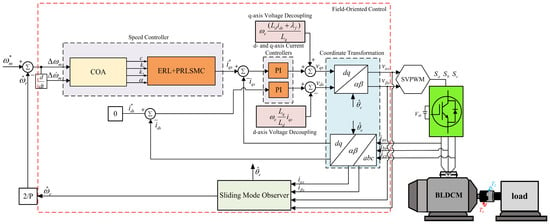
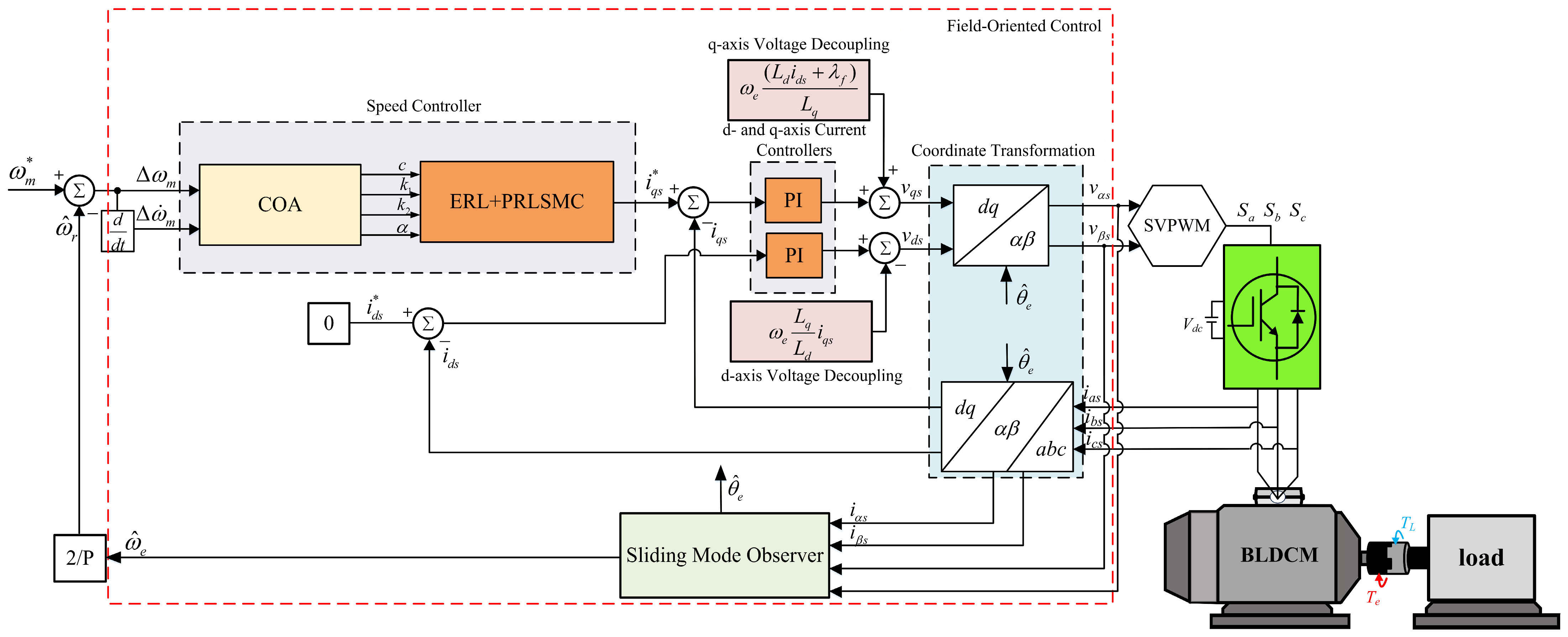
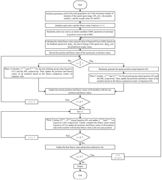
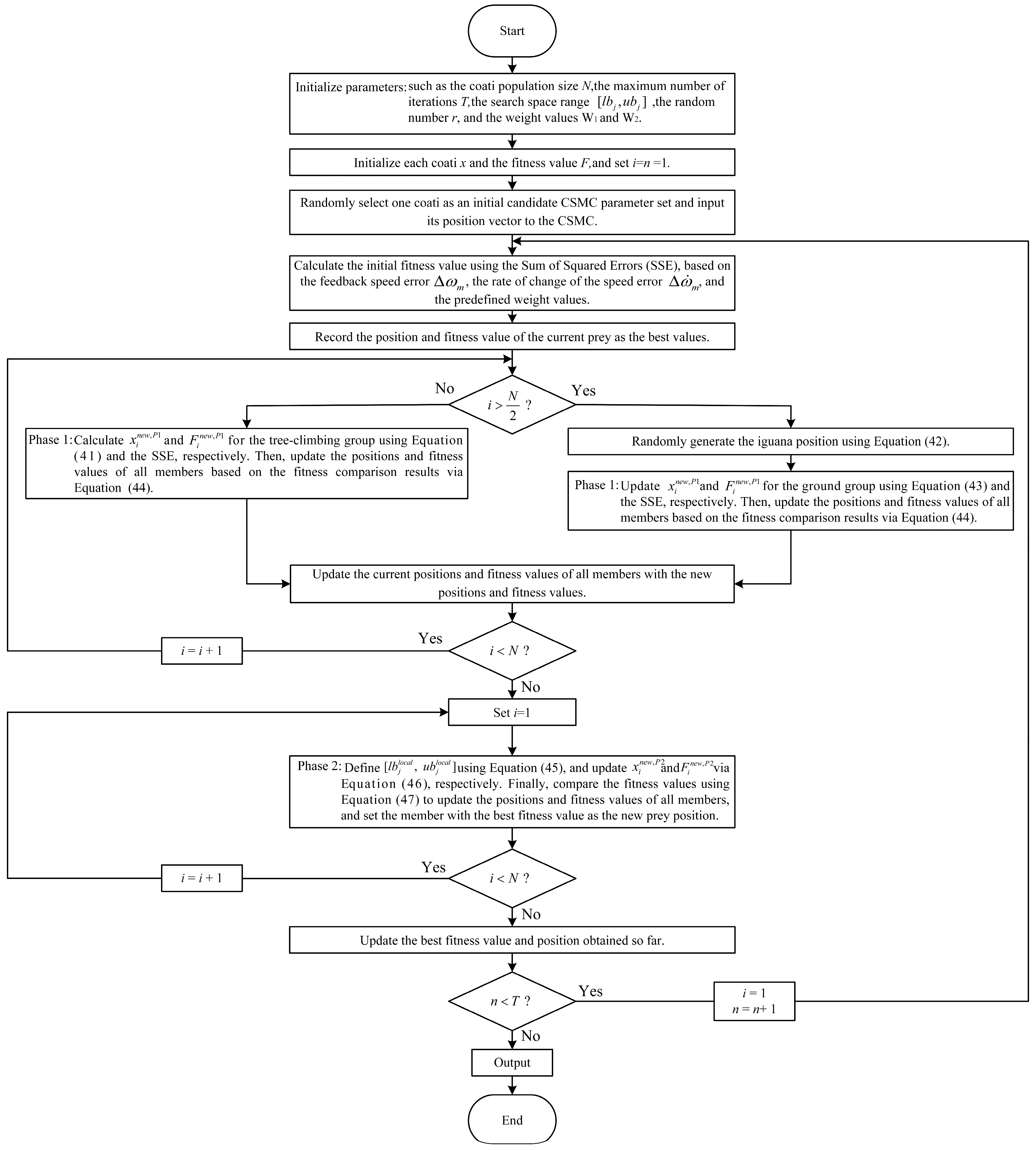
First, the global exploration capability of the first phase of the algorithm is exploited to identify potential optimal solutions, followed by the local exploitation mechanism of the second phase for detailed screening, so as to determine the final optimal parameter combination. The speed sensorless FOC architecture of the BLDCM drive system incorporating the COA combined with the power and exponential reaching law-based SMC is illustrated in Figure 2, while the steps of the COA for dynamically adjusting the gain parameters are detailed below, and the corresponding control flowchart is shown in Figure 3.
Figure 2.
Block diagram of the speed sensorless FOC architecture for the BLDCM drive system incorporating the COA combined with the CSMC.
Figure 3.
Control flowchart of the proposed novel COA.
- Step 1:
- Set the relevant parameters, including the coati population size N, the maximum number of iterations T, the search space range [], corresponding to the upper and lower bounds of the parameters , the random number , and the weight values and .
- Step 2:
- Initialize the position and fitness value F of each coati.
- Step 3:
- First, to establish the initial fitness reference, one coati individual is first randomly selected from the initialized population, and its position coordinates are input to the CSMC. Then, the initial fitness value is evaluated using the sum of squared error (SSE), in which the feedback speed error e and the rate of change in the speed error are considered with the predefined weighting factors and . These two weighting factors are used to indicate the relative contribution of each feature to the fitness evaluation. According to the sliding mode variable defined in Equation (21), the speed error plays the dominant role in the controller response, whereas the rate of change in the speed error provides an auxiliary correction effect. Therefore, = 0.6 and = 0.4 are selected, with . The fitness value is then computed by the SSE criterion, as formulated in Equation (48).where and are the speed error and the rate of change in the speed error of the i-th coati in the n-th iteration, respectively.
- Step 4:
- Record the current position and fitness value of the prey as the best solution found so far.
- Step 5:
- Execute the first-stage hunting behavior. The population is divided into the tree-climbing group and the ground-waiting group. Equations (41) and (43) are used to calculate the new position and new fitness value of the i-th coati in the j-th dimension. Subsequently, Equation (44) is applied to compare the corresponding fitness value with the current fitness value , thereby determining whether to update the position of the i-th coati. If , the position of the i-th coati is updated to ; otherwise, its position remains unchanged.
- Step 6:
- Record the new positions and new fitness values of all population members as their current positions and fitness values.
- Step 7:
- Execute the second-stage predator-avoidance behavior. In this stage, Equation (45) is first used to reduce the local search range as the number of iterations increases. Then, Equation (46) is used to recalculate the position and fitness value of the i-th coati in the j-th dimension. Subsequently, Equation (47) is applied to compare the corresponding fitness value with the current fitness value , thereby determining whether to update the position of the i-th coati. If , the position of the i-th coati is updated to ; otherwise, its position remains unchanged. Afterward, the individual with the best fitness value among all population members is designated as the new prey, i.e., .
- Step 8:
- Update the best fitness value and the best position obtained so far. If the number of iterations has reached the predefined maximum number of iterations, the iteration process is terminated, and the best position coordinate values are output as the four gain parameters of the CRL-based SMC to be tuned. Finally, the final output of the controller is determined using Equation (27).
To clarify the computational burden of the proposed online optimization, the COA is executed with a predefined population size, maximum iteration number, and search dimension. The detailed control-parameter settings are listed in Table 1. Since only four CRLSMC parameters are optimized in this study, the search dimension is fixed as D = 4. Therefore, the computational complexity of one COA update can be approximately expressed as O (N, T, D), where O denote the function of computational complexity notation, and N, T, and D denote the population size, maximum iteration number, and search dimension, respectively. After the predefined maximum number of iterations is completed, the best parameter set is output to the CRLSMC. Thus, the computational load is bounded and can be adjusted by selecting suitable values of N and T according to the available computation time of the digital controller. In the proposed implementation, the COA is executed at the speed-loop update rather than at every current-loop sampling instant. If the COA computation exceeds the available speed-loop computation time in practical hardware implementation, the previous best parameter set can be retained until the next update cycle to avoid interruption of the control output.
Table 1.
Parameter values adopted for the COA-CRLSMC of the proposed control scheme.
4. Simulation Results
In order to validate the performance of the proposed robust intelligent speed controller, the present work employs Matlab/Simulink R2024b to conduct simulation verification of the speed control performance of the BLDCM drive system. The simulation results are used to benchmark the proposed controller against other conventional and improved SMCs in terms of speed command tracking response and load regulation response. The motor used for testing is an AM-2200H permanent-magnet BLDCM [20] manufactured by Adlee Powertronic Co., Ltd. (Taichung, Taiwan), and its main parameters are listed in Table 2.
Table 2.
Specifications of the adopted BLDCM.
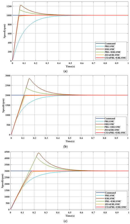
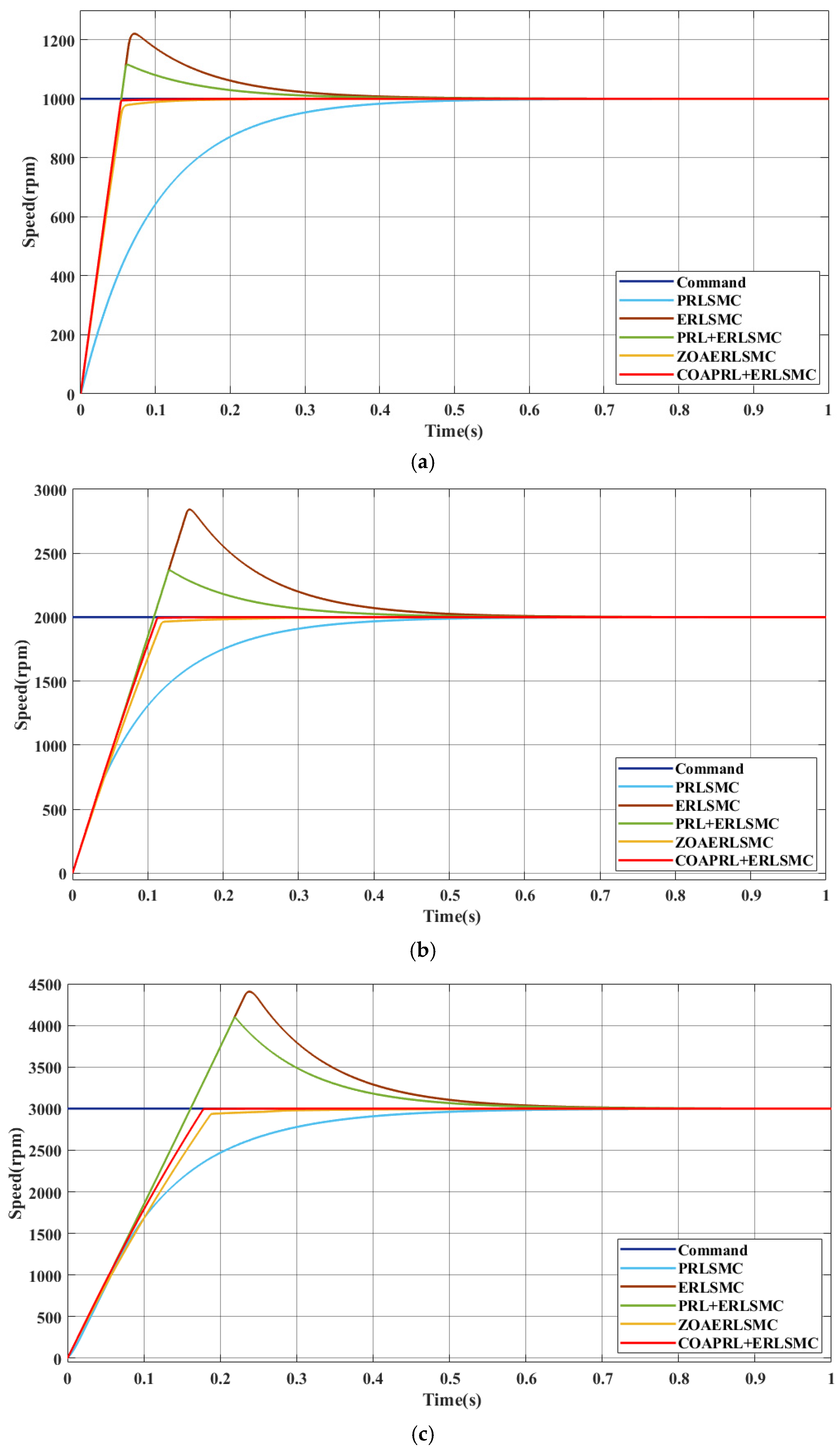
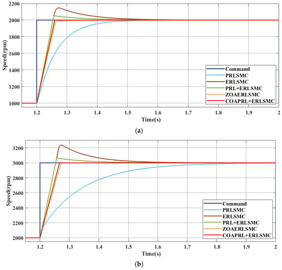
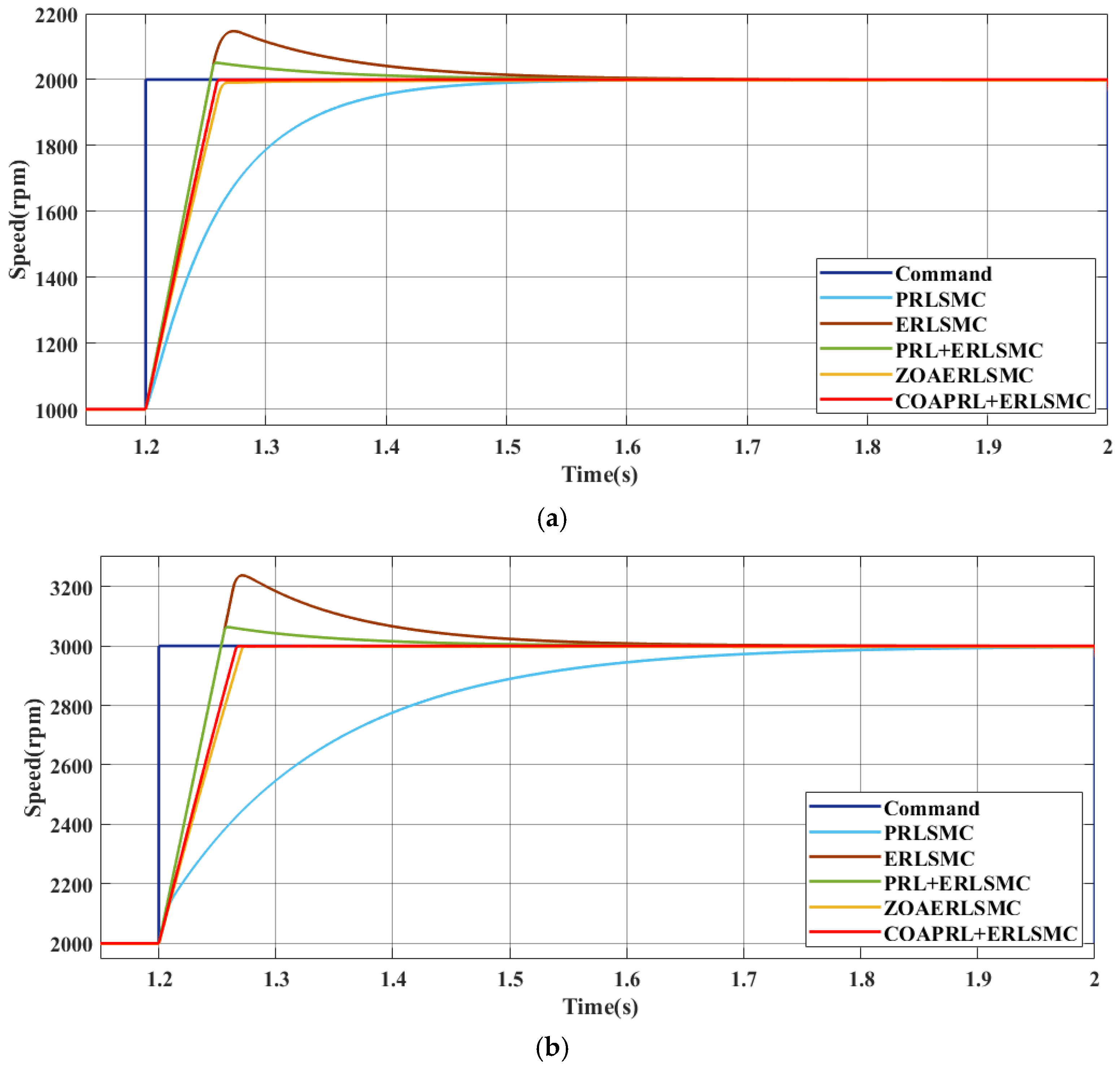
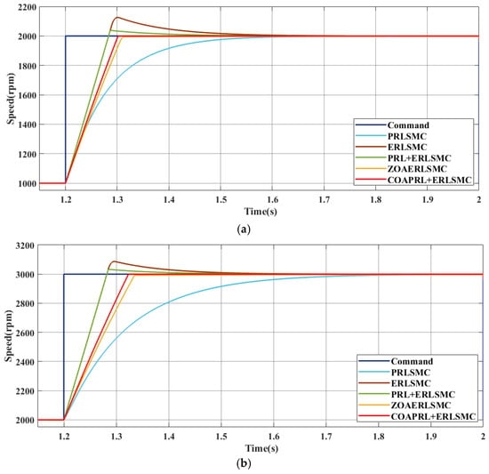
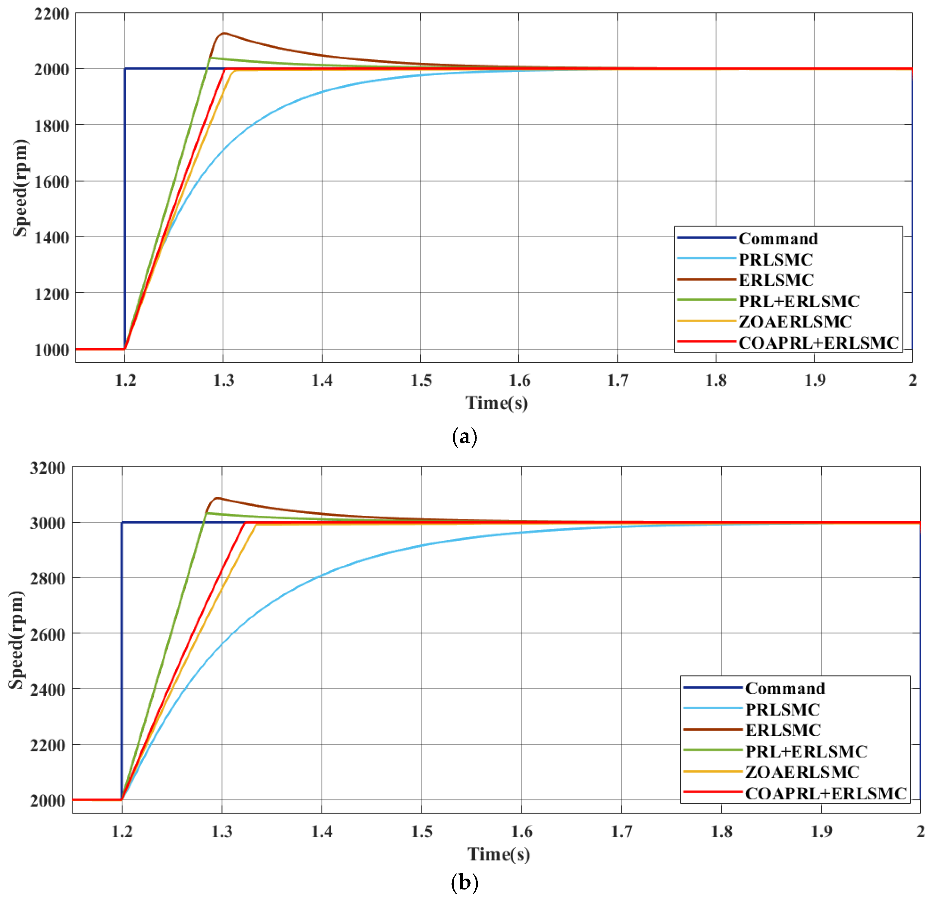
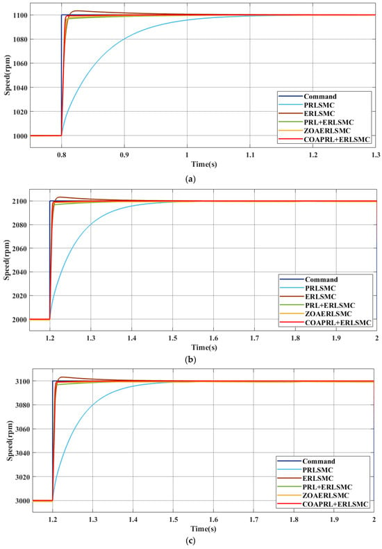
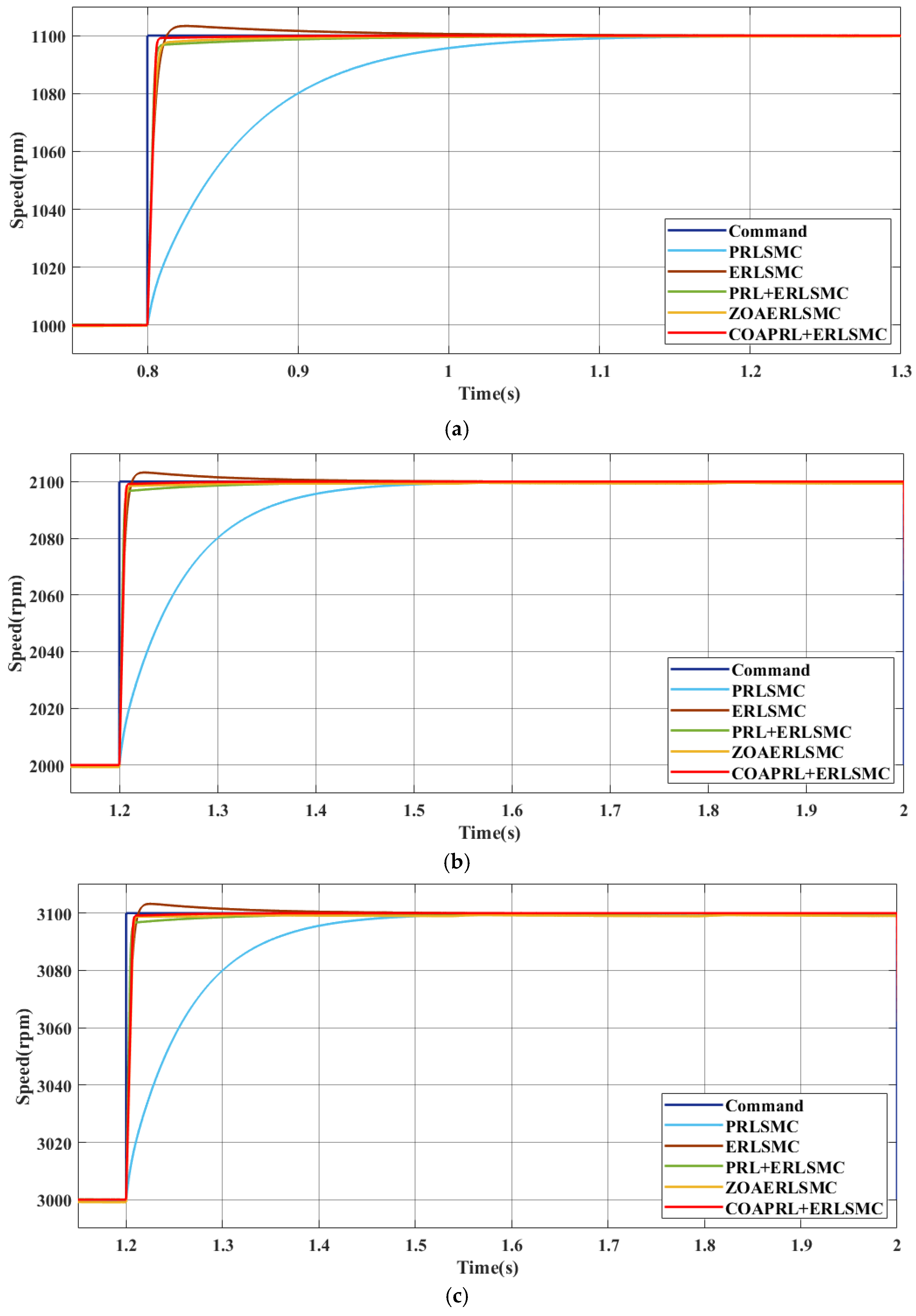
This paper compares the speed control performance of the BLDCM drive system based on the simulation results obtained using five controllers: the power reaching law sliding mode controller (PRLSMC), which adopts only the PRL; ERLSMC, which adopts only the ERL; the power and exponential reaching law sliding mode controller (PERLSMC), which combines the power and exponential reaching laws; the zebra optimization algorithm combined with exponential reaching law sliding mode controller (ZOAERLSMC); and the proposed coati optimization algorithm combined with power and exponential reaching law sliding mode controller (COAPERLSMC). Figure 4a–c present the simulated speed command tracking responses of the BLDCM under a constant load of , where the speed command ramps up from 0 rpm to 1000 rpm, 2000 rpm, and 3000 rpm, respectively. Figure 5a,b and Figure 6a,b illustrate the speed response results under load conditions of and , respectively. In these tests, the speed command increases from 1000 rpm to 2000 rpm as well as increases from 2000 rpm to 3000 rpm. In addition, to further verify the control performance of the proposed controller under small-amplitude speed command variations, Figure 7a–c present the speed response results under a constant load of . The speed command increases from 1000 rpm to 1100 rpm, increases from 2000 rpm to 2100 rpm, and increases from 3000 rpm to 3100 rpm, respectively. From the speed tracking responses shown in Figure 4, Figure 5, Figure 6 and Figure 7, it can be clearly observed that the proposed controller not only eliminates overshoot but also achieves the shortest speed command tracking time among the five controllers.
Figure 4.
Comparison of speed command tracking responses among the proposed COAPERLSMC, the ZOAERLSMC, the PERLSMC, the ERLSMC, and the PRLSMC under a load of , where the speed command increases from 0 rpm to different target speeds: (a) : 0 rpm→1000 rpm; (b) : 0 rpm→2000 rpm; (c) : 0 rpm→3000 rpm.
Figure 5.
Comparison of speed command tracking responses among the proposed COAPERLSMC, the ZOAERLSMC, the PERLSMC, the ERLSMC, and the PRLSMC under a load of , where the speed command varies under different operating conditions: (a) : 1000 rpm→2000 rpm; (b) : 2000 rpm→3000 rpm.
Figure 6.
Comparison of speed command tracking responses among the proposed COAPERLSMC, the ZOAERLSMC, the PERLSMC, the ERLSMC, and the PRLSMC under a load of , where the speed command varies under different operating conditions: (a) : 1000 rpm→2000 rpm; (b) : 2000 rpm→3000 rpm.
Figure 7.
Comparison of speed command tracking responses among the proposed COAPERLSMC, the ZOAERLSMC, the PERLSMC, the ERLSMC, and the PRLSMC under a load of , where the speed command undergoes small-amplitude variations under different operating conditions: (a) : 1000 rpm→1100 rpm; (b) : 2000 rpm→2100 rpm; (c) : 3000 rpm→3100 rpm.
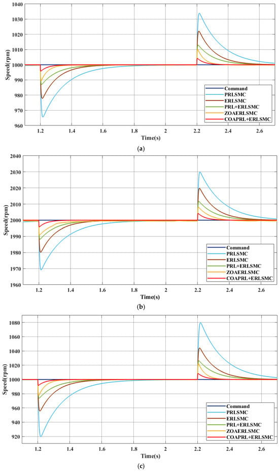
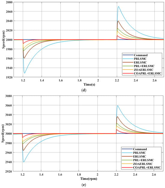
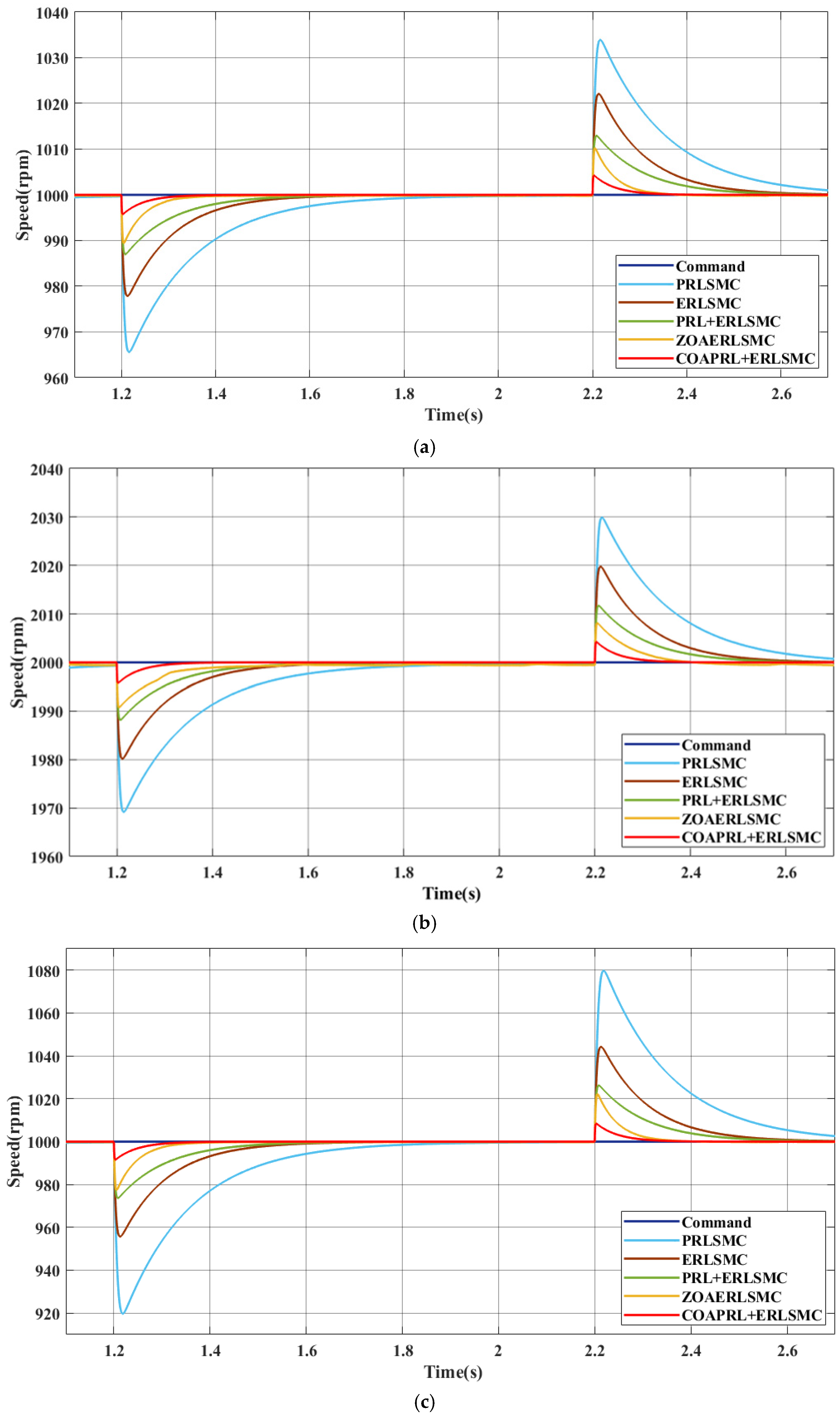
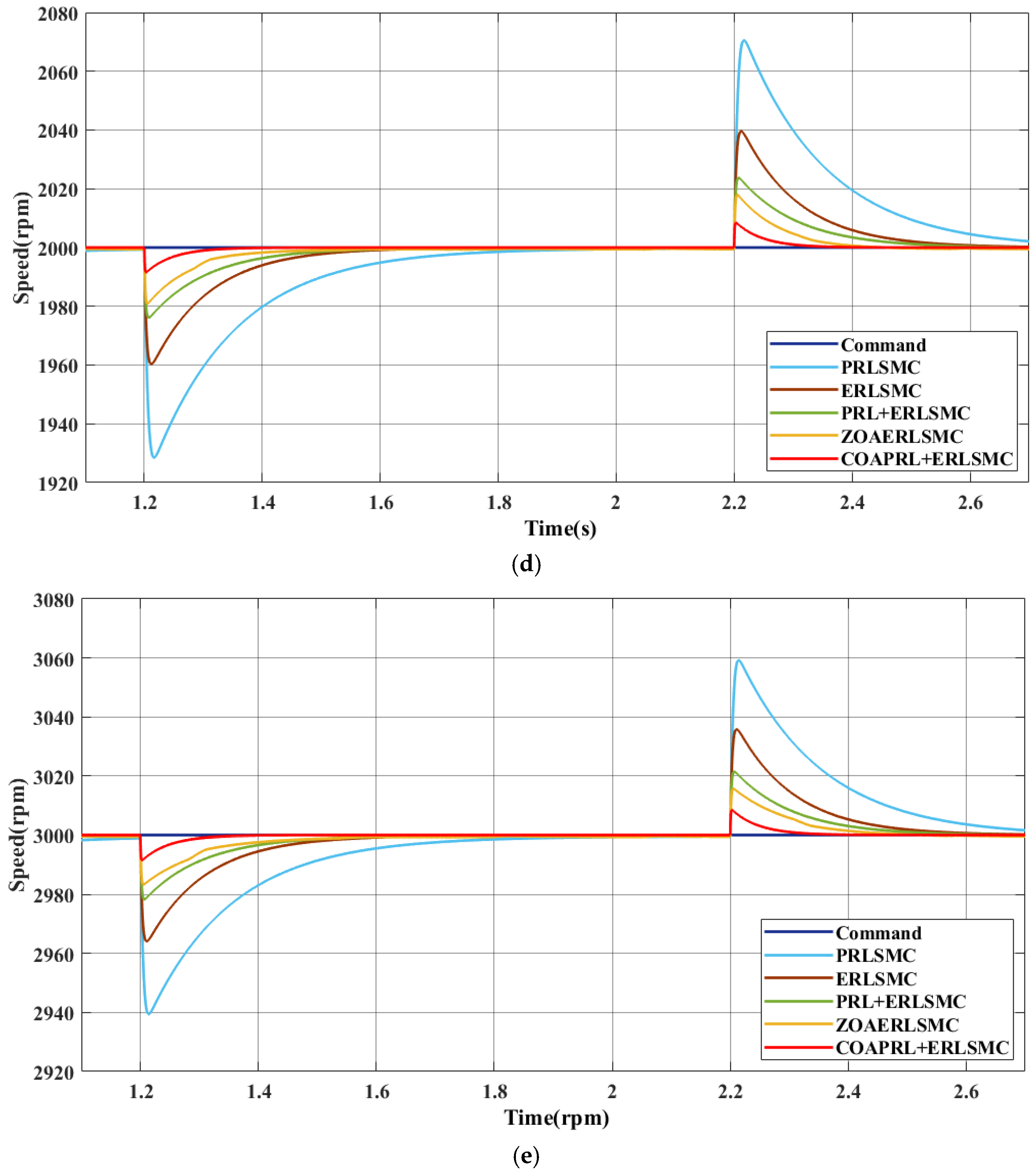
Figure 8a,b present the simulated load regulation responses at speed commands of 1000 rpm and 2000 rpm, respectively, under a load torque variation of = 0→1→0 . Figure 8c–e present the simulated load regulation responses at speed commands of 1000 rpm, 2000 rpm, and 3000 rpm, respectively, under a load torque variation of = 0→2→0 . In the load-regulation tests, the rated torque of the adopted BLDCM is . Therefore, the and load torques correspond to approximately 33.3% and 66.7% of the rated torque, respectively, and are used to represent light-load and heavy-load disturbances. The 0→1→0 and 0→2→0 load variations are applied to evaluate the speed drop and recovery capability of each controller under different load disturbance levels.
Figure 8.
Comparison of load regulation responses among the proposed COAPERLSMC, the ZOAERLSMC, the PERLSMC, the ERLSMC, and the PRLSMC under different speed commands, where the load torque is applied at 1.2 s and removed at 2.2 s: (a) : 1000 rpm, = 0→1→0 ; (b) : 2000 rpm, = 0→1→0 ; (c) : 1000 rpm, = 0→2→0 ; (d) : 2000 rpm, = 0 →2→0 ; (e) : 3000 rpm, = 0→2→0 .
Based on the simulation results, it can be observed that the SMC employing only the PRL exhibits a slower convergence speed when the system state is far from the sliding surface. As a result, a longer time is required for the motor speed to track the speed command. Moreover, under load variations, this controller produces the largest speed drop and exhibits a slow recovery response. In contrast, the SMC employing only the ERL improves the speed-command tracking response; however, it generates a relatively large overshoot, thereby affecting system stability. For the SMC combining the power and exponential reaching laws, although it integrates the advantages of both reaching laws, its parameter tuning is complex and difficult to optimize globally. Therefore, overshoot still occurs during the speed tracking response, and the recovery speed during load regulation remains insufficient. Compared with the above three SMC-based control methods, the ZOAERLSMC adopts an optimization algorithm to search for the controller parameters, and thus achieves improved tracking and load-regulation performance. However, its dynamic response and recovery capability under load regulation are still limited. To further support the above observations with quantitative data, Table 3, Table 4, Table 5, Table 6, Table 7 and Table 8 summarize the key simulation performance indices of the five controllers under different operating conditions. Table 3, Table 4, Table 5 and Table 6 present the speed-command tracking performance, where the evaluated indices are overshoot and settling time. Specifically, Table 3 and Table 4 show the tracking results under a load torque of for large and medium speed-command changes, respectively. Table 5 presents the tracking comparison under a load torque of , while Table 6 further evaluates small speed-command changes from 1000 rpm to 1100 rpm, 2000 rpm to 2100 rpm, and 3000 rpm to 3100 rpm. Table 7 and Table 8 present the load-regulation performance under step load disturbances of 0→1→0 and 0→2→0 , respectively, where the evaluated indices are speed drop and recovery time. From the quantitative results, the proposed COAPERLSMC achieves zero overshoot in all speed-command tracking tests, with settling times ranging from 0.05 s to 0.15 s. In the load-regulation tests, the speed drop of the proposed COAPERLSMC is limited to 4.3–4.7 rpm under the 0→1→0 load disturbance and 8.5–10.3 rpm under the 0→2→0 load disturbance. The corresponding recovery times are 0.08–0.10 s and 0.14–0.17 s, respectively. These results demonstrate that the proposed COAPERLSMC provides faster speed tracking, smaller speed deviation, and stronger load-disturbance suppression capability than the other four comparative controllers.
Table 3.
Speed tracking comparison under a load torque of for large and medium speed-command changes.
Table 4.
Speed tracking comparison under a load torque of for medium speed-command changes.
Table 5.
Speed tracking comparison under a load torque of for medium speed-command changes.
Table 6.
Speed tracking comparison under a load torque of for small speed-command changes.
Table 7.
Load regulation comparison for load = 0→1→0 .
Table 8.
Load regulation comparison for load = 0→2→0 .
5. Conclusions
The present study develops an SMC that integrates the COA with a CRL and is designed to replace the conventional P-I speed controller within the FOC architecture for BLDCM drive system speed regulation. The proposed intelligent speed controller employs the COA, which possesses strong global search capability, to address the complex parameter selection problem of the CRL-based SMC. The simulation results confirm that the proposed intelligent controller can effectively suppress the speed overshoot caused by the ERLSMC. The quantitative comparison presented in Table 3, Table 4, Table 5, Table 6, Table 7 and Table 8 further supports this result, showing that the proposed COAPERLSMC achieves zero overshoot in all speed-command tracking tests and provides smaller speed drop and faster recovery under load disturbances. It also overcomes the slow convergence speed and long load-regulation recovery time associated with the PRLSMC. Furthermore, in terms of both speed command tracking response and load regulation response, the proposed intelligent controller exhibits superior control performance compared with the existing ZOAERLSMC. In addition, the proposed algorithm has a clear logical structure and can achieve optimal parameter allocation without requiring a large amount of training data. Therefore, it demonstrates high engineering practicality and industrial application value. Nevertheless, the present study is mainly based on simulation verification. Since extremely low-speed operation and starting transients in sensorless BLDCM drives are strongly affected by rotor position and speed estimation accuracy, these conditions have not yet been fully investigated in this work. In future work, the proposed controller will be implemented on a practical BLDCM drive platform, and experimental tests will be conducted to verify its real-time feasibility, low-speed sensorless operation, robustness against motor-parameter variations, and load-disturbance suppression capability.
Author Contributions
Conceptualization, K.-H.C.; Methodology, K.-T.L.; Formal Analysis, K.-H.C.; Writing—Original Draft Preparation, K.-T.L.; Writing—Review and Editing, K.-H.C.; Project Administration, K.-H.C. All authors have read and agreed to the published version of the manuscript.
Funding
The authors gratefully acknowledge the support and funding of this project by the National Science and Technology Council, Taiwan, under Grant Number NSTC 114-2221-E-167-003-MY2.
Institutional Review Board Statement
Not applicable.
Informed Consent Statement
Not applicable.
Data Availability Statement
The original contributions presented in the study are included in the article, further inquiries can be directed to the corresponding author.
Conflicts of Interest
The authors declare no conflicts of interest.
Nomenclature
| Acronyms | |
| BLDCM | brushless DC motor |
| FOC | field-oriented control |
| P-I | proportional-integral |
| SMC | sliding mode controller |
| CSRL | constant speed reaching law |
| ERL | exponential reaching law |
| PRL | power reaching law |
| ET | extension theory |
| ZOA | zebra optimization algorithm |
| ERLSMC | exponential reaching law sliding mode controller |
| COA | coati optimization algorithm |
| CSMC | composite sliding mode controller |
| CRL | composite reaching law |
| PRLSMC | power reaching law sliding mode controller |
| ZOAERLSMC | zebra optimization algorithm combined with exponential reaching law sliding mode controller |
| COAPERLSMC | coati optimization algorithm combined with power and exponential reaching law sliding mode controller |
| Symbols | |
| stator flux linkages along the d-axis and q-axis | |
| constant excitation current | |
| mutual inductance | |
| permanent-magnet flux linkage | |
| stator voltages along the d-axis and q-axis | |
| stator resistance | |
| stator currents along the d-axis and q-axis | |
| electrical angular velocity | |
| stator inductances along the d-axis and q-axis | |
| electromagnetic torque | |
| number of poles | |
| moment of inertia | |
| mechanical angular velocity | |
| load torque | |
| viscous friction coefficient | |
| torque constant | |
| sliding mode variable | |
| sliding mode control gain | |
| state variables | |
| reaching law function | |
| Lyapunov candidate function | |
| constant speed reaching gain | |
| exponential reaching gain | |
| power reaching gain | |
| power exponent | |
| sign function | |
| exponential reaching gain of the composite reaching law | |
| power reaching gain of the composite reaching law | |
| auxiliary variable | |
| integration constant | |
| finite convergence time | |
| position of the i-th coati in the j-th dimension | |
| lower bound of the search space in the j-th dimension | |
| upper bound of the search space in the j-th dimension | |
| random number within the range [0, 1] | |
| coati population size | |
| new position of the i-th coati in the j-th dimension during first-stage hunting behavior | |
| randomly selected integer equal to 1 or 2 | |
| fitness value of the iguana landing position | |
| current fitness value of the i-th coati | |
| random landing position of the iguana in the j-th dimension | |
| candidate position of the i-th coati in the j-th dimension during predator-avoidance behavior | |
| current number of iterations | |
| maximum number of iterations | |
| weight values | |
| speed error of the i-th candidate solution at the n-th iteration | |
| rate of change in the speed error of the i-th candidate solution at the n-th iteration | |
References
- Lee, C.I.; Jang, G.H. Experimental Measurement and Simulated Verification of the Unbalanced Magnetic Force in Brushless DC Motors. IEEE Trans. Magn. 2008, 44, 4377–4380. [Google Scholar] [CrossRef] [Scilit]
- Mohanraj, D.; Aruldavid, R.; Verma, R.; Sathiyasekar, K.; Barnawi, A.B.; Chokkalingam, B.; Mihet-Popa, L. A Review of BLDC Motor: State of Art, Advanced Control Techniques, and Applications. IEEE Access 2022, 10, 54833–54869. [Google Scholar] [CrossRef] [Scilit]
- Fadli, M.R.; Furqani, J.; Musyasy, M.M.; Purwadi, A. Modelling of Field Orientation Control (FOC) Method in 120 kW Brushless DC (BLDC) Motor. In Proceedings of the 6th International Conference on Electric Vehicular Technology (ICEVT), Bali, Indonesia, 18–21 November 2019; pp. 383–389. [Google Scholar]
- Bairwa, B.; Murari, M.; Shahapur, M.; Kavya, M.R.; Khan, M.F. Speed Control of BLDC Motor Using PI Controller. In Proceedings of the International Conference for Advancement in Technology (ICONAT), Goa, India, 24–26 January 2023; pp. 1–6. [Google Scholar]
- Murali, S.B.; Rao, P.M. Adaptive Sliding Mode Control of BLDC Motor Using Cuckoo Search Algorithm. In Proceedings of the 2nd International Conference on Inventive Systems and Control (ICISC), Coimbatore, India, 19–20 January 2018; pp. 989–993. [Google Scholar]
- Qi, C.; Xie, J.; Mao, H.; Xie, Q. Condition Assessment of Valve-side Bushing of Converter Transformer Based on Extension Theory. In Proceedings of the IEEE International Conference on High Voltage Engineering and Application (ICHVE), Beijing, China, 6–10 September 2020; pp. 1–4. [Google Scholar]
- Trojovská, E.; Dehghani, M.; Trojovský, P. Zebra Optimization Algorithm: A New Bio-inspired Optimization Algorithm for Solving Optimization Algorithm. IEEE Access 2022, 10, 49445–49473. [Google Scholar] [CrossRef] [Scilit]
- Chao, K.H.; Lin, Z.N. Extenics Theory-Based Speed Controller Design for a Brushless DC Motor Drive System. In Proceedings of the 2025 International Future Energy Electronics Conference (IFEEC), Bali, Indonesia, 19–21 November 2025; pp. 359–364. [Google Scholar]
- Chao, K.H.; Huang, K.H.; Guo, Y.H. Design of a Brushless DC Motor Drive System Controller Integrating the Zebra Optimization Algorithm and Sliding Mode Theory. Electronics 2025, 14, 3353. [Google Scholar] [CrossRef] [Scilit]
- Dehghani, M.; Montazeri, Z.; Trojovská, E.; Trojovský, P. Coati Optimization Algorithm: A New Bio-inspired Metaheuristic Algorithm for Solving Optimization Problems. Knowl.-Based Syst. 2023, 259, 110011. [Google Scholar] [CrossRef] [Scilit]
- Xie, T.; Kuai, Z.; Ye, X.; Zhu, L.; Guo, K.; Shi, S. Coordinate Conversions and Deviation Analysis in Multi-source Data Fusion. In Proceedings of the 2nd China International SAR Symposium (CISS), Shanghai, China, 3–5 November 2021; pp. 1–3. [Google Scholar]
- Liu, C.H. AC Motor Control: Principles of Vector Control and Direct Torque Control, 4th ed.; Donghua Book Company: Taipei, Taiwan, 2007. [Google Scholar]
- Van Der Broeck, H.W.; Skudelny, H.C.; Stanke, G.V. Analysis and Realization of a Pulse Width Modulator Based on Voltage Space Vectors. IEEE Trans. Ind. Appl. 1988, 24, 142–150. [Google Scholar] [CrossRef] [Scilit]
- Zuo, Y.; Lai, C.; Iyer, K.L.V. A Review of Sliding Mode Observer-Based Sensorless Control Methods for PMSM Drive. IEEE Trans. Power Electron. 2023, 38, 11352–11367. [Google Scholar] [CrossRef] [Scilit]
- Yeh, C.C. AC Motor Control and Simulation Technology, 2nd ed.; Wu-Nan Book Inc.: Taipei, Taiwan, 2024. [Google Scholar]
- Utkin, V.I. Variable Structure Systems with Sliding Modes. IEEE Trans. Autom. Contr. 1977, 22, 212–222. [Google Scholar] [CrossRef] [Scilit]
- Gao, W.B.; Hung, J.C. Variable Structure Control of Nonlinear Systems: A New Approach. IEEE Trans. Ind. Electron. 1993, 40, 45–55. [Google Scholar] [CrossRef] [Scilit]
- Shang, W.; Wang, H. PMSM Integral Sliding Mode Control Based on Improved Power Exponential Reaching Law. Sci. Rep. 2025, 15, 21450. [Google Scholar] [CrossRef] [Scilit] [PubMed]
- Lyapunov, A.M. The General Problem of the Stability of Motion. Int. J. Contr. 1992, 55, 531–773. [Google Scholar] [CrossRef] [Scilit]
- AM2200H BLDC Motor. Available online: https://www.adlee.com/zh-tw/product-552515/%E5%B7%A5%E6%A5%AD%E7%94%A8%E7%9B%B4%E6%B5%81%E7%84%A1%E5%88%B7%E9%A6%AC%E9%81%94.html (accessed on 8 May 2024).

Disclaimer/Publisher’s Note: The statements, opinions and data contained in all publications are solely those of the individual author(s) and contributor(s) and not of MDPI and/or the editor(s). MDPI and/or the editor(s) disclaim responsibility for any injury to people or property resulting from any ideas, methods, instructions or products referred to in the content. |
© 2026 by the authors. Licensee MDPI, Basel, Switzerland. This article is an open access article distributed under the terms and conditions of the Creative Commons Attribution (CC BY) license.