Stability-Certified ResNN-Based Consensus Control for Multi-Agent Systems via Certificate-by-Construction Training

Abstract

This paper develops a stability-certified distributed residual neural network (ResNN) controller for leaderless consensus of continuous-time first-order multi-agent systems over undirected connected graphs. Unlikeconventional linear protocols and post-training verification methods, the proposed framework combines nonlinear transient shaping with certificate feasibility throughout learning. Each agent uses relative state differences with neighboring agents and applies a shared ResNN policy composed of a linear diffusive backbone and a bias-free neural residual branch. A computable residual-gain bound yields a sufficient condition for global exponential consensus, with the certified rate determined by the backbone–residual gain margin and the algebraic connectivity of the graph. Spectral-norm projection and gain reparameterization preserve this condition after every training update. A complementary forward-Euler certificate provides an explicit step-size condition for exponentially convergent digital implementation. The controller is trained through differentiable closed-loop simulation using an objective that balances disagreement and control effort. Ournumerical results verify the certified decay bound, demonstrate competitive transient trade-offs against three baselines, and evaluate direct deployment across different graph topologies and network sizes.

1. Introduction

Distributed coordination of networked multi-agent systems (MASs) is a cornerstone of modern control, with applications in multi-robot teams, multi-UAV systems, and networked spacecraft [1,2,3,4]. Among various objectives, consensus and formation coordination provide canonical mechanisms for agreement, synchronization, and cooperative motion, and they admit scalable neighbor-based distributed control laws; see, e.g., [5,6,7,8,9,10]. Despite the mature solvability theory, achieving fast and well-shaped transients in practical networks remains nontrivial: fixed-form linear protocols often require careful gain/weight tuning [11], they can be conservative under uncertainties and delays [12,13], and they face an inherent disagreement–effort trade-off governed by a small set of parameters [14,15]. Related studies have also investigated adaptive event-triggered tracking and communication-efficient cooperative control [16,17,18].

Learning-enabled controllers, especially neural network (NN) policies, offer a powerful avenue to improve transient behavior and adapt to complex dynamics [19,20]. However, embedding NNs into feedback loops raises a central concern: while expressive, NN-induced nonlinear maps are difficult to analyze and may jeopardize closed-loop stability and robustness [21,22]. In addition, unconstrained training may violate safety constraints during exploration or become fragile in the presence of unmodeled perturbations [23,24].

These concerns have spurred extensive research on stability-guaranteed learning, where learning is coupled with explicit certificates, e.g., Lyapunov-based constructions and convex relaxations [21,22,25,26,27]. On the one hand, verification-oriented tools such as IQC/QC analysis can certify stability/robustness for feedback interconnections containing NN blocks [21,22,28]. On the other hand, Lipschitz-constrained architectures and spectral-norm regularization/normalization provide practical handles to control NN gains during training [29,30,31]. Existing stability-certified neural control methods either verify a trained controller using quadratic constraints or Lyapunov inequalities, or they incorporate stability conditions into controller learning [21,22,25,26,27]. Most of these methods focus on a single plant. For example, the neural observer in [32] combines a model-based observer with a neural correction term for an uncertain nonlinear system. These results do not directly guarantee consensus of a graph-coupled multi-agent closed loop or preserve certificate feasibility throughout training.

To address this gap, we propose a distributed ResNN controller composed of a linear diffusive backbone and a bias-free neural residual branch. Each agent applies the same policy to its local diffusive signal. A computable residual-gain bound yields a sufficient condition for global exponential consensus, whose certified rate depends on the backbone–residual gain margin and the algebraic connectivity of the graph. A complementary forward-Euler condition provides an explicit step-size bound for convergent digital implementation. Spectral-norm projection and gain reparameterization preserve the continuous-time certificate after each training update, while the digital-stability margin is checked before closed-loop rollouts. Global graph information is used only during offline training, whereas online execution requires only local relative-state information and the shared policy. Our numerical experiments compared the proposed controller with representative baselines, verified the certified decay bound, and examined direct deployment across different graph topologies and network sizes.

The main contributions are summarized as follows:

• We propose a distributed ResNN consensus controller that combines a linear diffusive backbone with a bias-free neural residual branch. Unlike a fixed-gain linear protocol, the proposed policy provides state-dependent transient shaping while preserving the neighbor-based information pattern.
• We derive a sufficient certificate for global exponential consensus, explicitly relating the certified rate to the backbone–residual gain margin and the algebraic connectivity of the graph. We also establish a forward-Euler step-size condition for exponentially convergent digital implementation.
• We develop a certificate-by-construction training method that keeps the sufficient consensus condition satisfied after every optimization update. Spectral-norm projection bounds the residual gain, and gain reparameterization maintains a strictly positive certificate margin before the next closed-loop rollout.

The rest of this paper is organized as follows. Section 2 introduces notation and graph preliminaries; Section 3 formulates the problem and presents the ResNN-based controller; Section 4 establishes the consensus certificate; Section 5 describes the certificate-by-construction training procedure; and Section 6 and Section 7 present our numerical experiments and conclude the paper.

2. Preliminaries and Notation

2.1. Notation

Let $\mathbb{R}$ denote the set of real numbers and ${\mathbb{Z}}_{\ge 0}$ denote the set of non-negative integers. For a scalar $a\in \mathbb{R}$, $\left|a\right|$ denotes its absolute value. For a vector $v\in {\mathbb{R}}^n$, $\parallel v\parallel$ denotes the Euclidean norm. For a matrix M, ${\parallel M\parallel }_2$ denotes the spectral norm and $M^{\top }$ denotes the transpose. For a symmetric matrix M, $M⪰0$ ($M\succ 0$) means that M is positive semidefinite (positive definite). The identity matrix of dimension n is denoted by $I_n$, and the all-one vector of dimension N is denoted by ${\mathbf{1}}_N$. For vectors $v_1,\dots ,v_N$ with compatible dimensions, define $\mathrm{col}(v_1,\dots ,v_N):={\left[v_1^{\top },\dots ,v_N^{\top }\right]}^{\top }$. Throughout the paper, the bracketed superscript $\left[\mathcal{l}\right]$ denotes a layer index (not a power).

A mapping $f:{\mathbb{R}}^m\to {\mathbb{R}}^p$ is (globally) Lipschitz if there exists $\zeta \ge 0$ such that

$$\parallel f\left(x\right)-f\left(y\right)\parallel \le \zeta \parallel x-y\parallel ,\forall x,y\in {\mathbb{R}}^m.$$

The (global) Lipschitz constant is defined by

$$\mathrm{Lip}\left(f\right):=\inf \left\{\zeta \ge 0:\parallel f\left(x\right)-f\left(y\right)\parallel \le \zeta \parallel x-y\parallel ,\forall x,y\in {\mathbb{R}}^m\right\}.$$

2.2. Graph Theoretic Preliminaries

Consider an undirected weighted graph $\mathcal{G}=(\mathcal{V},\mathcal{E},\mathcal{A})$ with node set $\mathcal{V}=\{1,\dots ,N\}$, edge set $\mathcal{E}\subseteq \mathcal{V}\times \mathcal{V}$, and a symmetric adjacency matrix $\mathcal{A}=\left[a_{ij}\right]$ satisfying $a_{ij}=a_{ji}\ge 0$ and $a_{ij}>0$ if and only if $(i,j)\in \mathcal{E}$. The neighbor set of agent i is ${\mathcal{N}}_i:=\{j\in \mathcal{V}\mid (i,j)\in \mathcal{E}\}$. Let $D=\mathrm{diag}(d_1,\dots ,d_N)$ be the degree matrix with $d_i:={\sum }_{j=1}^N{a}_{ij}$ and define the Laplacian matrix $L:=D-\mathcal{A}$.

For an undirected connected graph, L is symmetric and positive semi-definite with $L{\mathbf{1}}_N=0$. We denote its eigenvalues by $0={\lambda }_1<{\lambda }_2\le \cdots \le {\lambda }_N$, where ${\lambda }_2$ is the algebraic connectivity and ${\lambda }_N$ is the largest Laplacian eigenvalue.

3. Problem Formulation and ResNN-Based Controller

Consider a leaderless multi-agent system consisting of N agents indexed by $\mathcal{V}=\{1,\dots ,N\}$. The communication topology is described by a graph $\mathcal{G}$.

Assumption 1.

The graph $\mathcal{G}$ is undirected and connected.

Each agent is modeled as a first-order integrator:

$${\dot{x}}_i\left(t\right)=u_i\left(t\right),i=1,\dots ,N,t\ge 0,$$

(1)

where $x_i\left(t\right)\in \mathbb{R}$ is the agent state and $u_i\left(t\right)\in \mathbb{R}$ is the control input.

Remark 1.

The first-order integrator model is adopted to present the certificate-by-construction mechanism in a transparent setting. Under this model, the effects of the residual-gain bound, the certified margin, and the graph connectivity can be isolated without introducing additional model-dependent conditions. Therefore, the present theoretical result should be interpreted as a foundational result for the proposed training principle rather than as a general certificate for arbitrary multi-agent dynamics. Extending the framework to higher-order, heterogeneous, or nonlinear agents requires a stabilizing model-based backbone and a residual branch whose gain can be incorporated into an appropriate Lyapunov or input–output stability condition. Such extensions generally lead to matrix-valued certificates rather than the scalar gain-dominance condition used in this paper.

Motivated by the backbone–residual decomposition used in the neural observer of [32], we parameterize the distributed controller by a residual neural network (ResNN) policy [33], denoted by ${\pi }_{\theta }(·)$, where $\theta$ collects the architecture hyperparameters and trainable parameters. Each agent computes the local diffusive signal

$$s_i\left(t\right)=\sum _{j\in {\mathcal{N}}_i}{a}_{ij}\left(x_j\left(t\right)-x_i\left(t\right)\right)$$

and applies a shared policy

$$u_i\left(t\right)={\pi }_{\theta }\left(s_i\left(t\right)\right),i=1,\dots ,N.$$

(2)

This information pattern is fully decentralized, since only relative state differences with neighboring agents are required online.

All agents share the same scalar policy map ${\pi }_{\theta }:\mathbb{R}\to \mathbb{R}$, parameterized as

$${\pi }_{\theta }\left(v\right)=kv+{\varphi }_{\widehat{\theta }}\left(v\right),$$

(3)

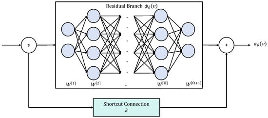
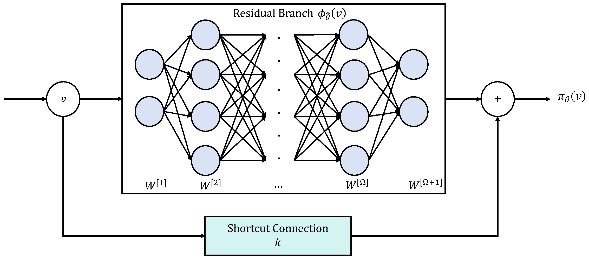
where $k\in \mathbb{R}$ is a shortcut gain and ${\varphi }_{\widehat{\theta }}(·)$ is a bias-free multilayer perceptron (MLP) residual branch; see Figure 1. The ResNet-style skip connection makes the linear diffusive backbone explicit and isolates the learnable residual correction.

Figure 1. ResNN policy parameterization (3): a linear shortcut $kv$ plus a bias-free MLP residual term ${\varphi }_{\widehat{\theta }}\left(v\right)$.

Let $\sigma :\mathbb{R}\to \mathbb{R}$ denote the neuron activation, and assume $\sigma \left(0\right)=0$ and $\mathrm{Lip}\left(\sigma \right)\le 1$. For any $n\in {\mathbb{Z}}_{\ge 1}$, define the componentwise lifting ${\sigma }^{\left[n\right]}:{\mathbb{R}}^n\to {\mathbb{R}}^n$ by

$${\sigma }^{\left[n\right]}\left(z\right):=\mathrm{col}\left(\sigma \left(z_1\right),\dots ,\sigma \left(z_n\right)\right),z\in {\mathbb{R}}^n.$$

The residual branch has $\mathsf{\Omega }$ hidden layers with widths ${\left\{n_{\mathcal{l}}\right\}}_{\mathcal{l}=1}^{\mathsf{\Omega }}$ and scalar input/output $n_0=n_{\mathsf{\Omega }+1}=1$. Define $h^{\left[0\right]}=v$, and for $\mathcal{l}=1,\dots ,\mathsf{\Omega }$,

$$z^{\left[\mathcal{l}\right]}=W^{\left[\mathcal{l}\right]}{h}^{[\mathcal{l}-1]},h^{\left[\mathcal{l}\right]}={\sigma }^{\left[n_{\mathcal{l}}\right]}\left(z^{\left[\mathcal{l}\right]}\right),$$

(4)

where $W^{\left[\mathcal{l}\right]}\in {\mathbb{R}}^{n_{\mathcal{l}}\times n_{\mathcal{l}-1}}$. The output layer is linear,

$${\varphi }_{\widehat{\theta }}\left(v\right)=W^{[\mathsf{\Omega }+1]} h^{\left[\mathsf{\Omega }\right]},W^{[\mathsf{\Omega }+1]}\in {\mathbb{R}}^{1\times n_{\mathsf{\Omega }}}.$$

(5)

No bias terms are used in any layer; together with $\sigma \left(0\right)=0$, this yields ${\varphi }_{\widehat{\theta }}\left(0\right)=0$. The parameter set of the ResNN policy ${\pi }_{\theta }(·)$ is

$$\theta :=(\mathcal{S},\widehat{\theta },k)=\left(\mathsf{\Omega },{\left\{n_{\mathcal{l}}\right\}}_{\mathcal{l}=0}^{\mathsf{\Omega }+1},W^{\left[1\right]},\dots ,W^{[\mathsf{\Omega }+1]},k\right),$$

(6)

where $\mathcal{S}:=\left(\mathsf{\Omega },{\left\{n_{\mathcal{l}}\right\}}_{\mathcal{l}=0}^{\mathsf{\Omega }+1}\right)$ denotes the architecture hyperparameters and $\widehat{\theta }={\left\{W^{\left[\mathcal{l}\right]}\right\}}_{\mathcal{l}=1}^{\mathsf{\Omega }+1}$ collects the residual-branch weight matrices.

Assumption 2 (Residual gain bound).

The residual mapping ${\varphi }_{\widehat{\theta }}:\mathbb{R}\to \mathbb{R}$ satisfies ${\varphi }_{\widehat{\theta }}\left(0\right)=0$ and there exists a constant $\beta \ge 0$ such that

$$|{\varphi }_{\widehat{\theta }}\left(v\right)|\le \beta |v|,\forall v\in \mathbb{R}.$$

(7)

Remark 2.

Assumption 2 is naturally satisfied by the bias-free network architecture adopted in this work. Specifically, we implement ${\varphi }_{\widehat{\theta }}(·)$ as a bias-free MLP with pointwise activations $\sigma (·)$ obeying $\sigma \left(0\right)=0$ and $\mathrm{Lip}\left(\sigma \right)\le 1$. In this case, the residual mapping satisfies the global gain bound

$$|{\varphi }_{\widehat{\theta }}\left(v\right)|\le {\beta }_{\mathrm{ub}}(\widehat{\theta })\left|v\right|,\forall v\in \mathbb{R},$$

with the computable estimate ${\beta }_{\mathrm{ub}}(\widehat{\theta }):={\prod }_{\mathcal{l}=1}^{\mathsf{\Omega }+1}{\parallel W^{\left[\mathcal{l}\right]}\parallel }_2$. Therefore, (7) holds for any $\beta \ge {\beta }_{\mathrm{ub}}(\widehat{\theta })$. This bound is sufficient (not necessary) for Assumption 2, but it is computable and compatible with layerwise spectral control during training.

Stacking (2), the closed-loop dynamics of (1) can be written compactly as

$$\left\{\begin{array}{c}\dot{x}\left(t\right)=u\left(t\right),\hfill \\ u\left(t\right)=ks\left(t\right)+{\mathsf{\Phi }}_{\widehat{\theta }}\left(s\left(t\right)\right),\hfill \\ s\left(t\right)=-Lx\left(t\right),\hfill \end{array}\right.$$

(8)

where $x\left(t\right),u\left(t\right),s\left(t\right)\in {\mathbb{R}}^N$ are stacked vectors $x\left(t\right)=\mathrm{col}\left(x_1\left(t\right),\dots ,x_N\left(t\right)\right)$ (similarly for $u\left(t\right)$ and $s\left(t\right)$), and

$${\mathsf{\Phi }}_{\widehat{\theta }}\left(s\right):=\mathrm{col}\left({\varphi }_{\widehat{\theta }}\left(s_1\right),\dots ,{\varphi }_{\widehat{\theta }}\left(s_N\right)\right)$$

denotes the componentwise application of the scalar residual map ${\varphi }_{\widehat{\theta }}(·)$.

Define the consensus error for each agent as

$${\delta }_i\left(t\right):=x_i\left(t\right)-{\displaystyle \frac{1}{N}}{\displaystyle \sum _{j=1}^N}{x}_j\left(t\right),$$

and stack $\delta \left(t\right)=\mathrm{col}\left({\delta }_1\left(t\right),\dots ,{\delta }_N\left(t\right)\right)$. Then

$$\delta \left(t\right)=Hx\left(t\right),H:=I_N-{\displaystyle \frac{1}{N}}{\mathbf{1}}_N{\mathbf{1}}_N^{\top }.$$

(9)

Note that $\delta \left(t\right)=0$ if and only if $x\left(t\right)\in \mathrm{span}\left\{{\mathbf{1}}_N\right\}$, i.e., consensus achievement.

Our objective is to design the shared ResNN policy (2) satisfying Assumption 2 such that the leaderless MAS (1) over the undirected connected graph in Assumption 1 achieves consensus, i.e.,

$$\parallel \delta \left(t\right)\parallel \to 0\mathrm{as}t\to \infty ,$$

(10)

which is equivalent to pairwise agreement:

$$\underset{t\to \infty }{\lim }\left(x_i\left(t\right)-x_j\left(t\right)\right)=0,\forall i,j\in \mathcal{V}.$$

(11)

Remark 3.

The linear diffusive protocol $u_i\left(t\right)=k{s}_i\left(t\right)$ is a classical scalable design that guarantees leaderless consensus over undirected connected graphs [5,6]. Nevertheless, its transient behavior is governed by a single scalar gain k: increasing k can accelerate disagreement attenuation but also increases actuation magnitude, leading to a limited disagreement–effort trade-off within the linear family. The residual policy (2) augments this backbone with a state-dependent correction ${\varphi }_{\widehat{\theta }}(·)$ driven by the same local diffusive signal, enabling richer transient shaping (e.g., stronger feedback far from consensus and milder inputs near agreement) while preserving fully decentralized execution. Importantly, our subsequent analysis shows that such transient improvements can be pursued without compromising provable consensus as long as the residual mapping satisfies a verifiable global gain bound and the backbone gain maintains a positive certificate margin.

4. Consensus Certificate and Stability Analysis

This section establishes a verifiable exponential-consensus certificate for the continuous-time closed loop (8) under Assumption 1.

Lemma 1

(Spectral bounds of the Laplacian quadratic form [8]). Under Assumption 1, for any $x\in {\mathbb{R}}^N$ and $\delta =Hx$ with H in (9), it holds that

$${\lambda }_2{\parallel \delta \parallel }^2\le x^{\top }Lx\le {\lambda }_N{\parallel \delta \parallel }^2.$$

(12)

Theorem 1 (Exponential-consensus certificate).

Consider the continuous-time MAS (1) over an undirected connected graph (Assumption 1), controlled by the distributed ResNN policy (2) with ${\pi }_{\theta }\left(v\right)=kv+{\varphi }_{\widehat{\theta }}\left(v\right)$. Suppose Assumption 2 holds with some $\beta \ge 0$ and choose

$$k>\beta .$$

(13)

Then global leaderless consensus is achieved. Moreover, the disagreement energy $V\left(x\right)=\frac{1}{2}{x}^{\top }Lx$ decays exponentially as

$$V\left(x\left(t\right)\right)\le \exp \left(-2(k-\beta ){\lambda }_{2}t\right)V\left(x\left(0\right)\right),\forall t\ge 0.$$

(14)

Proof. 

Recall from (8) that $s\left(t\right)=-Lx\left(t\right)$ and $u\left(t\right)=ks\left(t\right)+{\mathsf{\Phi }}_{\widehat{\theta }}\left(s\left(t\right)\right)$. Under Assumption 2, for each component,

$$s_i{\varphi }_{\widehat{\theta }}\left(s_i\right)\ge -|s_i\left|\right|{\varphi }_{\widehat{\theta }}\left(s_i\right)|\ge -\beta |s_i{|}^2,$$

and summing over i yields

$$s^{\top }{\mathsf{\Phi }}_{\widehat{\theta }}\left(s\right)\ge -\beta {\parallel s\parallel }^2.$$

(15)

Consider the Lyapunov function

$$V\left(x\right):={\displaystyle \frac{1}{2}}{x}^{\top }Lx\ge 0.$$

(16)

Along trajectories of (8),

$$\begin{array}{cc}\hfill \dot{V}\left(x\left(t\right)\right)& =x{\left(t\right)}^{\top }L\dot{x}\left(t\right)={\left(-s\left(t\right)\right)}^{\top }u\left(t\right)\hfill \\ & =-{k\parallel s\left(t\right)\parallel }^2-s{\left(t\right)}^{\top }{\mathsf{\Phi }}_{\widehat{\theta }}\left(s\left(t\right)\right).\hfill \end{array}$$

Using (15) gives

$$\dot{V}\left(x\left(t\right)\right)\le -(k-\beta ){\parallel s\left(t\right)\parallel }^2.$$

(17)

Next, note that ${\parallel s\left(t\right)\parallel }^2={\parallel Lx\left(t\right)\parallel }^2=x{\left(t\right)}^{\top }{L}^{2}x\left(t\right)$ and $L^2⪰{\lambda }_{2}L$ for undirected connected graphs. Therefore,

$${\parallel s\left(t\right)\parallel }^2=x{\left(t\right)}^{\top }{L}^{2}x\left(t\right)\ge {\lambda }_{2}x{\left(t\right)}^{\top }Lx\left(t\right)=2{\lambda }_{2}V\left(x\left(t\right)\right).$$

(18)

Combining (17) and (18) yields

$$\dot{V}\left(x\left(t\right)\right)\le -2(k-\beta ){\lambda }_{2}V\left(x\left(t\right)\right).$$

Gronwall’s inequality gives (14), hence $V\left(x\right(t\left)\right)\to 0$ exponentially. Finally, by Lemma 1, $V\left(x\right(t\left)\right)\to 0$ implies $\parallel \delta \left(t\right)\parallel \to 0$, establishing leaderless consensus.    □

Remark 4.

The certified rate in (14) depends on the margin $(k-\beta )$ and the algebraic connectivity ${\lambda }_2$. A larger margin or larger ${\lambda }_2$ yields a faster certified decay. In implementation, $m=k-{\beta }_{\mathrm{ub}}$ measures the certified dominance of the linear backbone over the residual branch. A larger margin provides greater tolerance to residual-gain variation before the sufficient condition is lost.

Setting ${\varphi }_{\widehat{\theta }}\equiv 0$ reduces (2) to the classical linear diffusive protocol $u_i\left(t\right)=k{s}_i\left(t\right)$, for which Theorem 1 recovers the standard exponential consensus result [5,6].

5. Certificate-by-Construction Training via Differentiable Simulation

This section presents a certificate-by-construction training procedure for the distributed ResNN controller (2), aimed at improving transient performance while enforcing the sufficient condition in Theorem 1 at every optimization iteration.

5.1. Certificate-by-Construction Parameterization

Recall that ${\varphi }_{\widehat{\theta }}$ is implemented as a bias-free MLP with pointwise activation $\sigma (·)$ satisfying $\sigma \left(0\right)=0$ and $\mathrm{Lip}\left(\sigma \right)\le 1$. Using (4) and (5), for any $v,w\in \mathbb{R}$,

$$\begin{array}{cc}\hfill \parallel h^{\left[\mathcal{l}\right]}\left(v\right)-h^{\left[\mathcal{l}\right]}\left(w\right)\parallel & =\parallel {\sigma }^{\left[n_{\mathcal{l}}\right]}\left(W^{\left[\mathcal{l}\right]}{h}^{[\mathcal{l}-1]}\left(v\right)\right)-{\sigma }^{\left[n_{\mathcal{l}}\right]}\left(W^{\left[\mathcal{l}\right]}{h}^{[\mathcal{l}-1]}\left(w\right)\right)\parallel \hfill \\ \hfill & \le \mathrm{Lip}\left(\sigma \right)\parallel W^{\left[\mathcal{l}\right]}\left(h^{[\mathcal{l}-1]}\left(v\right)-h^{[\mathcal{l}-1]}\left(w\right)\right)\parallel \hfill \\ \hfill & \le {\parallel W^{\left[\mathcal{l}\right]}\parallel }_2\parallel h^{[\mathcal{l}-1]}\left(v\right)-h^{[\mathcal{l}-1]}\left(w\right)\parallel ,\hfill \end{array}$$

Iterating over $\mathcal{l}=1,\dots ,\mathsf{\Omega }$ and applying the output layer yields

$$\begin{array}{cc}\hfill |{\varphi }_{\widehat{\theta }}\left(v\right)-{\varphi }_{\widehat{\theta }}\left(w\right)|& \le \parallel W^{[\mathsf{\Omega }+1]}{\parallel }_2\parallel h^{\left[\mathsf{\Omega }\right]}\left(v\right)-h^{\left[\mathsf{\Omega }\right]}\left(w\right)\parallel \hfill \\ \hfill & \le \parallel W^{[\mathsf{\Omega }+1]}{\parallel }_2{\displaystyle \prod _{\mathcal{l}=1}^{\mathsf{\Omega }}}\parallel W^{\left[\mathcal{l}\right]}{\parallel }_2|v-w|\hfill \\ \hfill & =\left({\displaystyle \prod _{\mathcal{l}=1}^{\mathsf{\Omega }+1}}\parallel W^{\left[\mathcal{l}\right]}{\parallel }_2\right)|v-w|.\hfill \end{array}$$

Therefore, by defining

$${\beta }_{\mathrm{ub}}\left(\widehat{\theta }\right):={\displaystyle \prod _{\mathcal{l}=1}^{\mathsf{\Omega }+1}}\parallel W^{\left[\mathcal{l}\right]}{\parallel }_2,$$

(19)

and taking $w=0$, we obtain the global gain bound

$$\left|{\varphi }_{\widehat{\theta }}\left(v\right)\right|=|{\varphi }_{\widehat{\theta }}\left(v\right)-{\varphi }_{\widehat{\theta }}\left(0\right)|\le {\beta }_{\mathrm{ub}}(\widehat{\theta })\left|v\right|,\forall v\in \mathbb{R}.$$

In particular, we enforce a certificate margin by construction. Theorem 1 requires $k>\beta$, where $\beta$ is the (unknown) global gain bound of the residual map in Assumption 2. Since $\beta$ is generally intractable to compute for a neural network, we work with the computable upper bound ${\beta }_{\mathrm{ub}}\left(\widehat{\theta }\right)$ in (19) and maintain

$$k>{\beta }_{\mathrm{ub}}\left(\widehat{\theta }\right)$$

(20)

at every optimization iteration. This is achieved by coupling a projection step that controls ${\beta }_{\mathrm{ub}}\left(\widehat{\theta }\right)$ and a strictly feasible parameterization of k.

First, we parameterize the layerwise spectral-norm limits by

$$c_{\mathcal{l}}=c_{\min }+(c_{\max }-c_{\min })\mathrm{sig}\left({\nu }_{\mathcal{l}}\right),\mathcal{l}=1,\dots ,\mathsf{\Omega }+1,$$

(21)

where ${\nu }_{\mathcal{l}}$ are trainable scalars and $0<c_{\min }<c_{\max }$ are to be chosen. In (21), $\mathrm{sig}(·)$ denotes the logistic sigmoid function,

$$\mathrm{sig}\left(z\right):={\displaystyle \frac{1}{1+e^{-z}}},z\in \mathbb{R}.$$

After each gradient update, we enforce the layerwise spectral-norm constraints by the following projection (spectral clipping) [29,30,31],

$$W^{\left[\mathcal{l}\right]}\leftarrow \min \left\{1,{\displaystyle \frac{c_{\mathcal{l}}}{\parallel W^{\left[\mathcal{l}\right]}{\parallel }_2}}\right\}{W}^{\left[\mathcal{l}\right]},\mathcal{l}=1,\dots ,\mathsf{\Omega }+1,$$

(22)

so that $\parallel W^{\left[\mathcal{l}\right]}{\parallel }_2\le c_{\mathcal{l}}$ holds for all layers at every iteration. Then, given ${\beta }_{\mathrm{ub}}\left(\widehat{\theta }\right)$, we set

$$k\left(\kappa \right)={\beta }_{\mathrm{ub}}\left(\widehat{\theta }\right)+\ln \left(1+e^{\kappa }\right),$$

(23)

which guarantees $k\left(\kappa \right)-{\beta }_{\mathrm{ub}}\left(\widehat{\theta }\right)>0$ for all $\kappa \in \mathbb{R}$.

The unconstrained variables $\kappa$ and ${\nu }_{\mathcal{l}}$ are optimized directly, while (23) guarantees $k>{\beta }_{\mathrm{ub}}\left(\widehat{\theta }\right)$ and (21) ensures $c_{\mathcal{l}}\in (c_{\min },c_{\max })$. Together with spectral projection, these parameterizations maintain certificate feasibility after each update.

5.2. Differentiable Simulation and Rollout Objective

We train the ResNN-based controller end-to-end via differentiable simulation of the continuous-time closed loop (8) over a finite horizon $[0,T]$. The rollout objective is defined as

$$\mathcal{L}(\widehat{\theta },\kappa ,\nu ):={\mathbb{E}}_{x\left(0\right)\sim \mathcal{D}}\left[\mathcal{J}\left({\{x\left(t\right),u\left(t\right)\}}_{t\in [0,T]}\right)\right],$$

(24)

where $\mathcal{J}(·)$ encodes the desired transient performance criteria.

Remark 5.

The rollout functional $\mathcal{J}(·)$ can be tailored to different transient objectives (e.g., faster convergence, reduced actuation, or smoother inputs). Importantly, the proposed certificate-by-construction mechanism is agnostic to the specific choice of $\mathcal{J}(·)$: it enforces the certified margin condition $k>{\beta }_{\mathrm{ub}}\left(\widehat{\theta }\right)$ via gain parameterization and spectral projection, which in turn guarantees consensus under the sufficient condition of Theorem 1. For instance, one may use time-varying weights to emphasize early-time error reduction, add an input-variation penalty such as ${\int }_0^T{\parallel \dot{u}\left(t\right)\parallel }^2\mathrm{d}t$ to promote smoother actuation, or include a state-magnitude regularizer to discourage large excursions, e.g., ${\int }_0^T{\parallel x\left(t\right)\parallel }^2\mathrm{d}t$ (or ${\int }_0^T{\parallel \delta \left(t\right)\parallel }^2\mathrm{d}t$ when only the disagreement component is penalized).

In implementation, we approximate (24) using a fixed-step forward-Euler scheme [34,35]. Let $t_m=mh$ and choose K such that $T=Kh$. With $x\left[m\right]\approx x\left(t_m\right)$, the discretized closed loop is

$$\begin{array}{cc}\hfill x[m+1]& =x\left[m\right]+hu\left[m\right],\hfill \\ \hfill u\left[m\right]& =ks\left[m\right]+{\mathsf{\Phi }}_{\widehat{\theta }}\left(s\left[m\right]\right),\hfill \\ \hfill s\left[m\right]& =-Lx\left[m\right].\hfill \end{array}$$

(25)

Although Theorem 1 guarantees exponential consensus in continuous time, the Euler implementation requires an additional step-size condition.

Proposition 1 (Forward-Euler implementation certificate).

Suppose that the residual branch satisfies $|{\varphi }_{\widehat{\theta }}\left(v\right)|\le {\beta }_{\mathrm{ub}}\left|v\right|$ for all $v\in \mathbb{R}$ and that $k>{\beta }_{\mathrm{ub}}$. Define the digital-stability margin

$${\mu }_h^{\mathrm{ub}}:=k-{\beta }_{\mathrm{ub}}-{\displaystyle \frac{h{\lambda }_N}{2}}{(k+{\beta }_{\mathrm{ub}})}^2.$$

(26)

If ${\mu }_h^{\mathrm{ub}}>0$, equivalently,

$$0<h<{\displaystyle \frac{2(k-{\beta }_{\mathrm{ub}})}{{\lambda }_N{(k+{\beta }_{\mathrm{ub}})}^2}},$$

(27)

then the Euler-discretized closed loop (25) achieves exponential consensus. In particular,

$$V\left(x\left[m\right]\right)\le {\rho }_h^{m}V\left(x\left[0\right]\right),{\rho }_h:=1-2h{\mu }_h^{\mathrm{ub}}{\lambda }_2\in [0,1).$$

(28)

Proof. 

Using $V\left(x\right)=\frac{1}{2}{x}^{\top }Lx$ and (25), the one-step variation of V is

$$\begin{array}{cc}\hfill V\left(x\right[m+1\left]\right)-V\left(x\right[m\left]\right)& =hx{\left[m\right]}^{\top }Lu\left[m\right]+{\displaystyle \frac{h^2}{2}}u{\left[m\right]}^{\top }Lu\left[m\right]\hfill \\ \hfill & =-hs{\left[m\right]}^{\top }u\left[m\right]+{\displaystyle \frac{h^2}{2}}u{\left[m\right]}^{\top }Lu\left[m\right].\hfill \end{array}$$

(29)

The residual-gain bound gives $-s{\left[m\right]}^{\top }u\left[m\right]\le -(k-{\beta }_{\mathrm{ub}}){\parallel s\left[m\right]\parallel }^2$. Moreover, $\parallel u\left[m\right]\parallel \le (k+{\beta }_{\mathrm{ub}})\parallel s\left[m\right]\parallel$ and $u{\left[m\right]}^{\top }Lu\left[m\right]\le {\lambda }_N{\parallel u\left[m\right]\parallel }^2$. Hence,

$$u{\left[m\right]}^{\top }Lu\left[m\right]\le {\lambda }_N{(k+{\beta }_{\mathrm{ub}})}^2{\parallel s\left[m\right]\parallel }^2.$$

Substituting these bounds into (29) yields

$$V\left(x[m+1]\right)-V\left(x\left[m\right]\right)\le -h{\mu }_h^{\mathrm{ub}}{\parallel s\left[m\right]\parallel }^2,$$

(30)

where ${\mu }_h^{\mathrm{ub}}$ is defined in (26). Since ${\parallel s\left[m\right]\parallel }^2=x{\left[m\right]}^{\top }{L}^{2}x\left[m\right]\ge 2{\lambda }_{2}V\left(x\left[m\right]\right)$, (30) gives

$$V\left(x[m+1]\right)\le \left(1-2h{\mu }_h^{\mathrm{ub}}{\lambda }_2\right)V\left(x\left[m\right]\right).$$

(31)

It remains to verify that the coefficient in (31) lies in $[0,1)$. Define

$$\xi :={\displaystyle \frac{h{\lambda }_N{(k+{\beta }_{\mathrm{ub}})}^2}{k-{\beta }_{\mathrm{ub}}}}.$$

Under (27), $\xi \in (0,2)$, and

$$0<2h{\mu }_h^{\mathrm{ub}}{\lambda }_2={\displaystyle \frac{{\lambda }_2}{{\lambda }_N}}{\left({\displaystyle \frac{k-{\beta }_{\mathrm{ub}}}{k+{\beta }_{\mathrm{ub}}}}\right)}^2\xi (2-\xi )\le 1.$$

(32)

Therefore, ${\rho }_h=1-2h{\mu }_h^{\mathrm{ub}}{\lambda }_2\in [0,1)$. Recursively applying (31) yields (28).    □

The step size h is chosen such that ${\mu }_h^{\mathrm{ub}}>0$. After each spectral projection, ${\beta }_{\mathrm{ub}}$ and k are recomputed, and the digital-stability margin is verified before the next rollout. A positive margin guarantees exponential consensus of the Euler-discretized closed-loop trajectories, but it does not imply global convergence of the nonconvex training problem. The resulting certificate-by-construction training procedure is summarized in Algorithm 1.

Algorithm 1 Certificate-by-construction training via differentiable simulation

1: Input: Laplacian L, integration step h, horizon K $(T=Kh)$, weight $\gamma$, bounds $(c_{\min },c_{\max })$, and optimizer stepsize.   2: Initialize: weights $\widehat{\theta }={\left\{W^{\left[\mathcal{l}\right]}\right\}}_{\mathcal{l}=1}^{\mathsf{\Omega }+1}$ and scalars $\kappa$ and $\nu ={\left\{{\nu }_{\mathcal{l}}\right\}}_{\mathcal{l}=1}^{\mathsf{\Omega }+1}$.   3: Compute ${\left\{c_{\mathcal{l}}\right\}}_{\mathcal{l}=1}^{\mathsf{\Omega }+1}$ via (21) and apply spectral clipping (22).   4: Compute ${\beta }_{\mathrm{ub}}\left(\widehat{\theta }\right)$ and set k via (19) and (23).   5: Compute ${\mu }_h^{\mathrm{ub}}$ via (26) and verify ${\mu }_h^{\mathrm{ub}}>0$.   6: for each training iteration do   7:     Compute ${\left\{c_{\mathcal{l}}\right\}}_{\mathcal{l}=1}^{\mathsf{\Omega }+1}$, ${\beta }_{\mathrm{ub}}\left(\widehat{\theta }\right)$, and k.   8:     Sample a mini-batch of initial conditions $x\left[0\right]\sim \mathcal{D}$.   9:     for $m=0$ to $K-1$ do 10:         $s\left[m\right]\leftarrow -Lx\left[m\right]$. 11:         $u\left[m\right]\leftarrow ks\left[m\right]+{\mathsf{\Phi }}_{\widehat{\theta }}\left(s\left[m\right]\right)$. 12:         $x[m+1]\leftarrow x\left[m\right]+hu\left[m\right]$. 13:     end for 14:     Evaluate $\mathcal{L}(\widehat{\theta },\kappa ,\nu )$ using (24). 15:     Perform a tentative gradient update by backpropagating through the rollout. 16:     Recompute ${\left\{c_{\mathcal{l}}\right\}}_{\mathcal{l}=1}^{\mathsf{\Omega }+1}$ and apply spectral clipping (22). 17:     Recompute ${\beta }_{\mathrm{ub}}\left(\widehat{\theta }\right)$ and update k. 18:     Recompute ${\mu }_h^{\mathrm{ub}}$; if ${\mu }_h^{\mathrm{ub}}\le 0$, reject the tentative update and retain the previous feasible iterate. 19: end for 20: Output: projected weights $\widehat{\theta }$ and shortcut gain k satisfying ${\mu }_h^{\mathrm{ub}}>0$.

Remark 6.

Algorithm 1 is consistent with the CTDE principle [36]. Let $C_{\varphi }:={\sum }_{\mathcal{l}=1}^{\mathsf{\Omega }+1}{n}_{\mathcal{l}}{n}_{\mathcal{l}-1}$ denote the dominant cost of one ResNN forward pass. For a mini-batch of size B and rollout horizon K, differentiable simulation and backpropagation have complexity $\mathcal{O}\left(BK\left(\right|\mathcal{E}|+N{C}_{\varphi })\right)$ under a sparse graph implementation. The residual-gain computation, spectral projection, digital-margin evaluation, and gain reparameterization are all performed offline. During online deployment, agent i only computes its local diffusive signal and evaluates the shared policy, with complexity $\mathcal{O}(d_i+C_{\varphi })$, where $d_i$ is its local degree. Thus, the proposed certificate mechanism introduces no online certification step and no additional communication overhead.

6. Numerical Experiments

For this section, we evaluated the transient behavior of the proposed ResNN-based consensus controller trained by the certificate-by-construction procedure in Section 5. All simulations implemented the decentralized control law, under which each agent uses only relative state information from its neighbors.

6.1. Experimental Setup

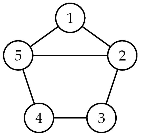
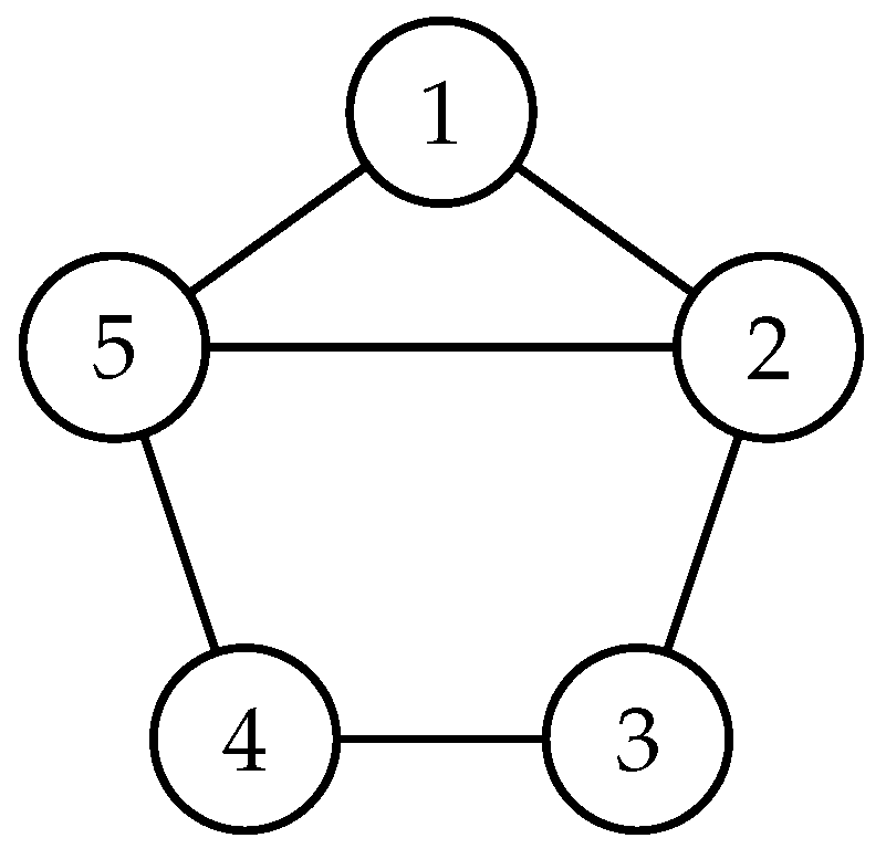
We considered the MAS (1) controlled by the distributed ResNN-based controller (2). We used a fixed undirected connected graph with $N=5$ agents and unit edge weights, shown in Figure 2. Its Laplacian eigenvalues were ${\lambda }_2=1.381966$ and ${\lambda }_N=4.618034$.

Figure 2. Communication topology used in simulations ($N=5$, undirected, unit edge weights).

To instantiate the functional $\mathcal{J}(·)$ in (24), we used the quadratic disagreement–effort trade-off

$$\mathcal{J}={\int }_0^T\left({\displaystyle \frac{1}{N}}{\parallel \delta \left(t\right)\parallel }^2+\gamma {\displaystyle \frac{1}{N}}{\parallel u\left(t\right)\parallel }^2\right)\mathrm{d}t,$$

(33)

where $\gamma \ge 0$ weights the control effort and $\delta \left(t\right)$ is defined in (9). We set $\gamma$ by loss-scale normalization at initialization so that the disagreement and effort terms had comparable magnitudes, which yielded $\gamma =0.127842$.

We adopted the ResNN parameterization (3) with $\mathsf{\Omega }=2$ hidden layers and widths $(n_0,n_1,n_2,n_3)=(1,16,16,1)$, using ReLU activations. The controller was trained for 2000 iterations following Algorithm 1, with the hyperparameters summarized in Table 1.

Table 1. Key hyperparameters used in Section 6.

Quantity	Value
Number of agents N	5
Graph	fixed connected undirected
Integrator step h	$0.001$
Evaluation horizon	$T=5$ (grid length $K=5000$)
Initial condition distribution	$x_i\left(0\right)\sim \mathrm{Uniform}[-2,2]$ (i.i.d.)
ResNN hidden layers $\mathsf{\Omega }$	2
Layer widths $(n_0,n_1,n_2,n_3)$	$(1,16,16,1)$
Activation $\sigma (·)$	ReLU
Loss weight $\gamma$	$0.127842$
Batch size (initial conditions)	64
Optimizer	Adam, learning rate ${10}^{-3}$
Training iterations	2000
Number of test trials $N_{\mathrm{test}}$	200

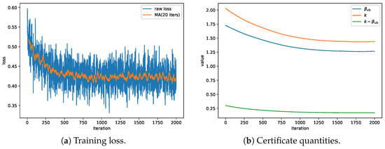
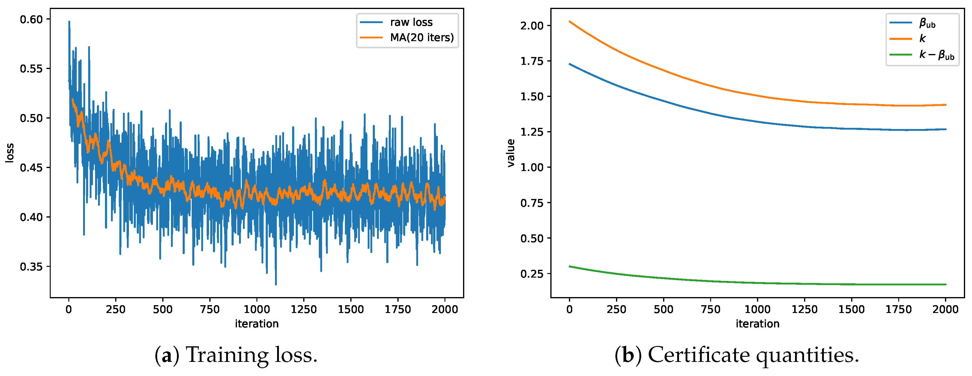
The training loss stabilized, and the learned gain k maintained a strictly positive certified margin $m=k-{\beta }_{\mathrm{ub}}$, as shown in Figure 3.

Figure 3. Training diagnostics of the proposed certificate-by-construction method: (a) training loss versus iterations, smoothed over 20 iterations; (b) evolution of the shortcut gain k and residual-gain bound ${\beta }_{\mathrm{ub}}$. The certified margin $m=k-{\beta }_{\mathrm{ub}}$ remained strictly positive throughout the training.

6.2. Baselines, Metrics, and Main Results

We compared the proposed ResNN-based controller against:

• BL1 (Linear, same gain): $u_i\left(t\right)=k{s}_i\left(t\right)$, where k was exported by the proposed controller (Table 2).
• BL2 (Linear, tuned gain): $u_i\left(t\right)=k_{\mathrm{lin}}{s}_i\left(t\right)$, where $k_{\mathrm{lin}}$ was selected by grid search to minimize the same objective (33) on a validation set with ${\varphi }_{\widehat{\theta }}\equiv 0$; we obtained $k_{\mathrm{lin}}=1.05$.
• BL3 (Unconstrained ResNN): the same ResNN architecture and rollout objective were used, but both the spectral clipping step (22) and the margin-enforcing shortcut-gain parameterization (23) were removed.

Table 2. Certificate diagnostics of the proposed controller and baselines.

Method	k	${\mathit{\beta }}_{\mathbf{ub}}$	$\mathit{m}=\mathit{k}-{\mathit{\beta }}_{\mathbf{ub}}$	Condition $\mathit{k}>{\mathit{\beta }}_{\mathbf{ub}}$
Ours	$1.44006$	$1.26715$	$0.172917$	Feasible
BL1	$1.44006$	0	$1.44006$	Feasible (linear)
BL2	$1.05$	0	$1.05$	Feasible (linear)
BL3	$2.0$	$5.1353$	$-3.1353$	Not certified

Consistent with (33), we evaluated the transient performance by the following metrics:

$$\begin{array}{cc}\hfill J_x& :={\int }_0^T{\displaystyle \frac{1}{N}}{\parallel \delta \left(t\right)\parallel }^2\mathrm{d}t,\hfill \\ \hfill J_u& :={\int }_0^T{\displaystyle \frac{1}{N}}{\parallel u\left(t\right)\parallel }^2\mathrm{d}t,\hfill \\ \hfill J_{\mathrm{total}}& :=J_x+\gamma J_u.\hfill \end{array}$$

(34)

Here, $J_x$ quantifies the accumulated disagreement energy over $[0,T]$, $J_u$ quantifies the accumulated control effort, and $J_{\mathrm{total}}$ is the loss-aligned composite score balancing disagreement and effort via $\gamma$. Table 2 summarizes the certificate diagnostics of the four controllers.

For the trained controller on the original graph, the selected step $h=0.001$ gave ${\mu }_h^{\mathrm{ub}}=0.15599>0$. Therefore, by Proposition 1, the Euler-discretized closed-loop implementation is exponentially convergent.

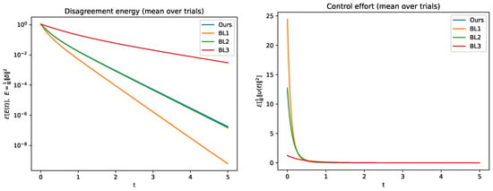
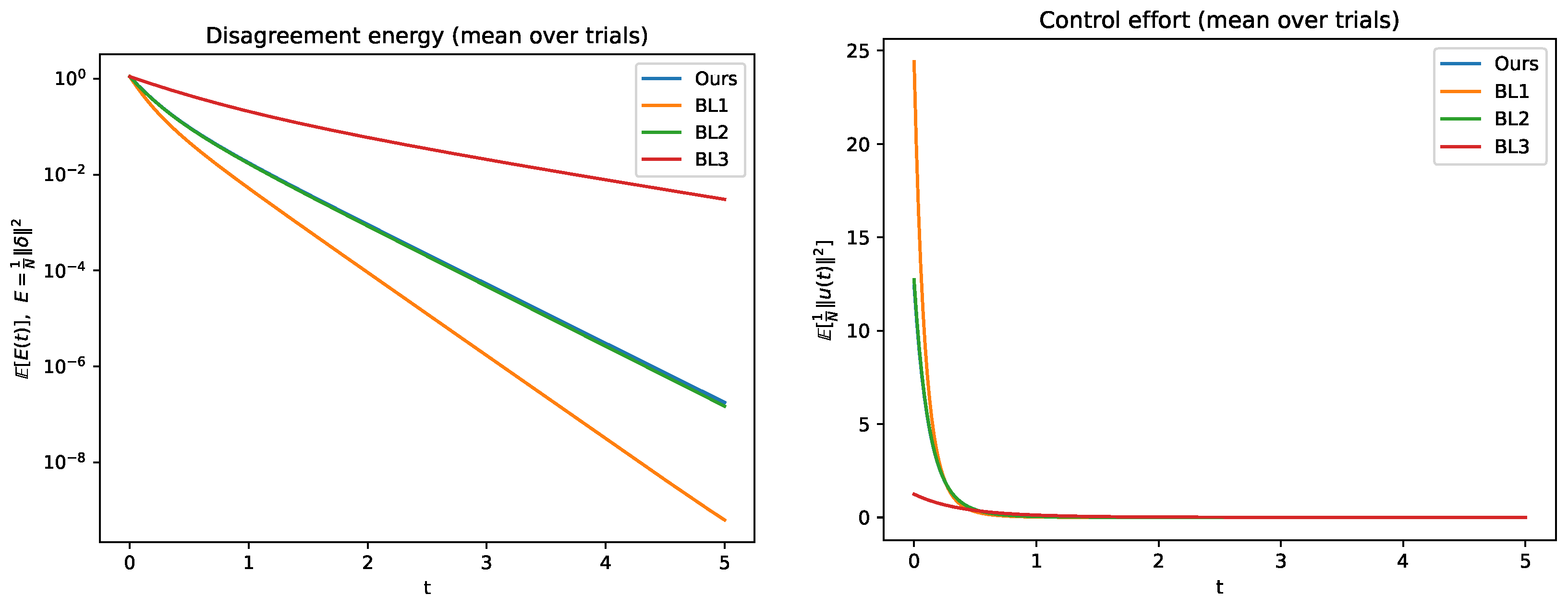
Figure 4 compares the mean disagreement energy and the mean control effort over time. Table 3 reports the aggregate metrics (mean ± std over $N_{\mathrm{test}}=200$ trials).

Figure 4. Transient responses under the proposed controller and baselines. Left: mean disagreement $\mathbb{E}\left[\frac{1}{N}{\parallel \delta \left(t\right)\parallel }^2\right]$ versus time; Right: mean effort $\mathbb{E}\left[\frac{1}{N}{\parallel u\left(t\right)\parallel }^2\right]$ versus time.

Table 3. Summary of transient performance over $[0,T]$ (mean ± std over $N_{\mathrm{test}}=200$ trials). Best (smallest) values in each column are highlighted in bold.

Method	${\mathit{J}}_{\mathit{x}}$	${\mathit{J}}_{\mathit{u}}$	${\mathit{J}}_{\mathbf{total}}$
Ours	$0.218\pm 0.131$	$1.721\pm 0.908$	$\mathbf{0}.\mathbf{438}\pm \mathbf{0}.\mathbf{216}$
BL1	$\mathbf{0}.\mathbf{156}\pm \mathbf{0}.\mathbf{093}$	$2.416\pm 1.274$	$0.464\pm 0.226$
BL2	$0.213\pm 0.128$	$1.760\pm 0.928$	$\mathbf{0}.\mathbf{438}\pm \mathbf{0}.\mathbf{217}$
BL3	$0.684\pm 0.409$	$\mathbf{0}.\mathbf{544}\pm \mathbf{0}.\mathbf{287}$	$0.754\pm 0.430$

Compared with BL1, the proposed controller reduced the control effort from $2.416$ to $1.721$, although BL1 achieved a smaller disagreement cost. The proposed controller and BL2 attained nearly identical $J_{\mathrm{total}}$ values, so no strict superiority over BL2 is claimed. Since BL2 is linear, ${\beta }_{\mathrm{ub}}=0$ and its gain condition was trivially satisfied.

The certificate-related comparison was therefore made with BL3, which used the same ResNN architecture without spectral clipping or gain reparameterization. BL3 yielded $k-{\beta }_{\mathrm{ub}}=-3.1353$ and was not certified, while also producing a larger disagreement cost and composite score. Thus, the main advantage of the proposed method is certificate-preserving nonlinear policy learning rather than a uniformly lower $J_{\mathrm{total}}$ than every tuned linear controller.

6.3. Transient Trade-Off Shaping by Sweeping $\gamma$

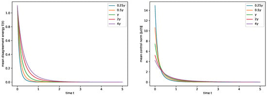
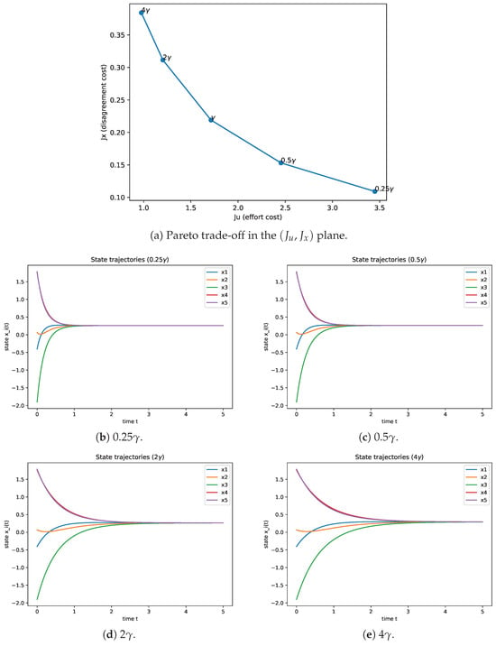
We further demonstrated that the proposed framework can generate a family of controllers with different transient trade-offs by varying the effort weight $\gamma$ in the instantiated objective (33). With the architecture and training procedure fixed, we re-trained a controller family $\Gamma =\{0.25\gamma ,0.5\gamma ,\gamma ,2\gamma ,4\gamma \}$ and evaluated all the controllers on the same test set described in Section 6.1. All the controllers obtained in the $\gamma$ sweep satisfied $k>{\beta }_{\mathrm{ub}}$ and ${\mu }_h^{\mathrm{ub}}>0$.

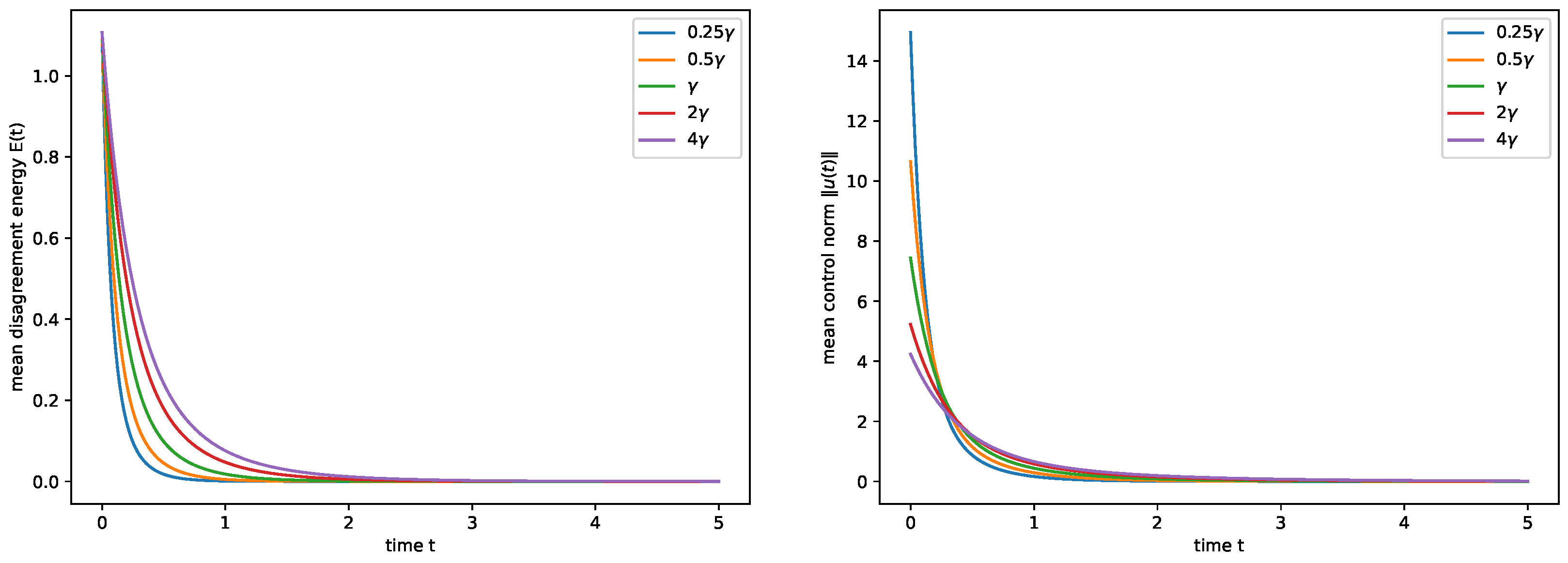
Figure 5 shows that smaller $\gamma$ yielded faster disagreement attenuation at the cost of larger effort, whereas larger $\gamma$ reduced effort but slowed convergence, forming a clear Pareto-type trade-off.

Figure 5. Sweep over $\gamma$: mean disagreement energy and control effort curves.

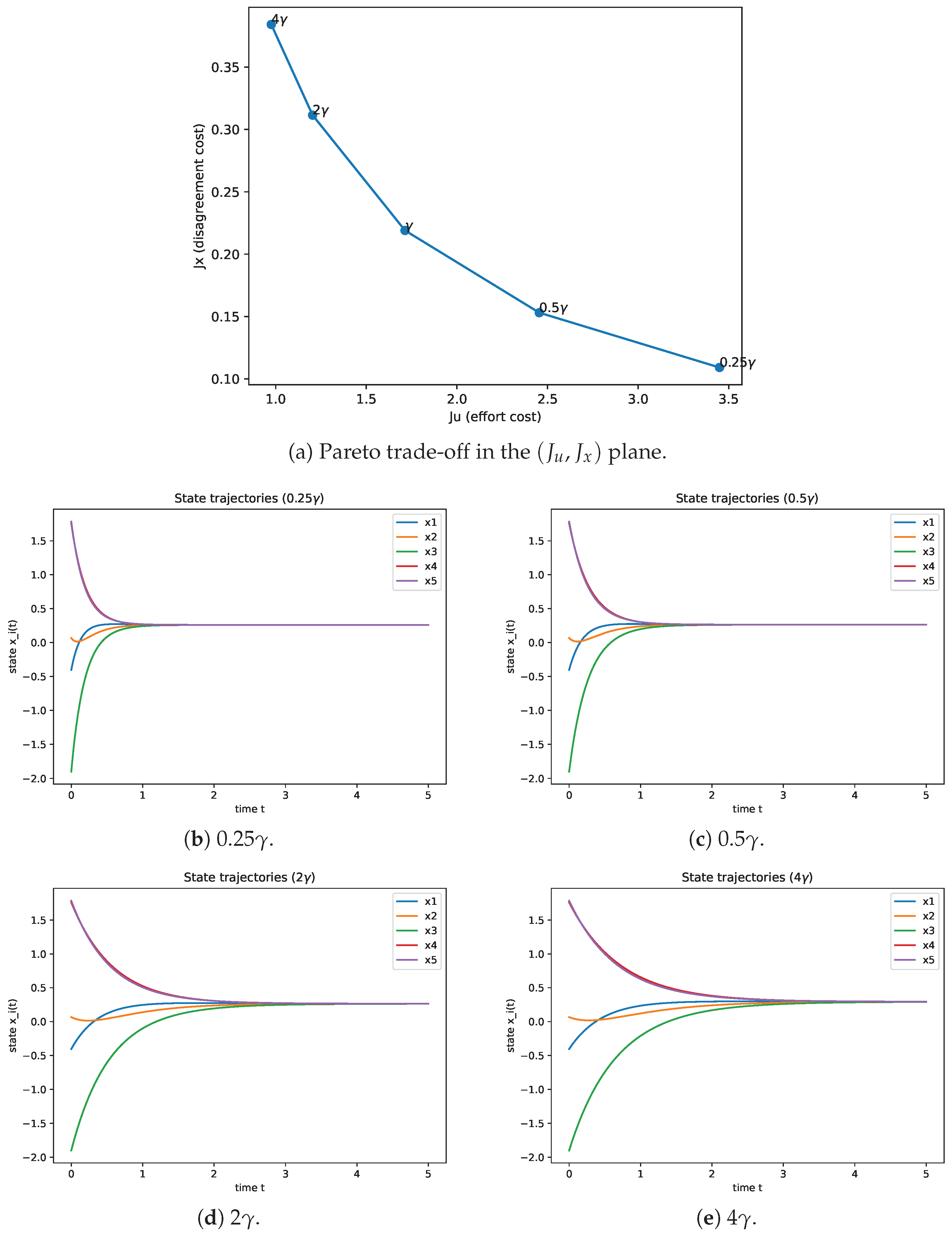
Figure 6a visualizes the trade-off in the $(J_u,J_x)$ plane, while Figure 6b–e shows representative state trajectories under different effort weights.

Figure 6. Transient trade-off shaping under different effort weights: (a) Pareto visualization of the $\gamma$ sweep in the $(J_u,J_x)$ plane; (b–e) representative state trajectories for $0.25\gamma$, $0.5\gamma$, $2\gamma$, and $4\gamma$, respectively.

6.4. Verification of the Certified Convergence Rate

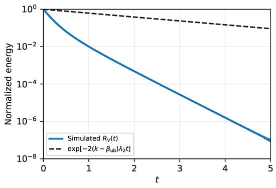
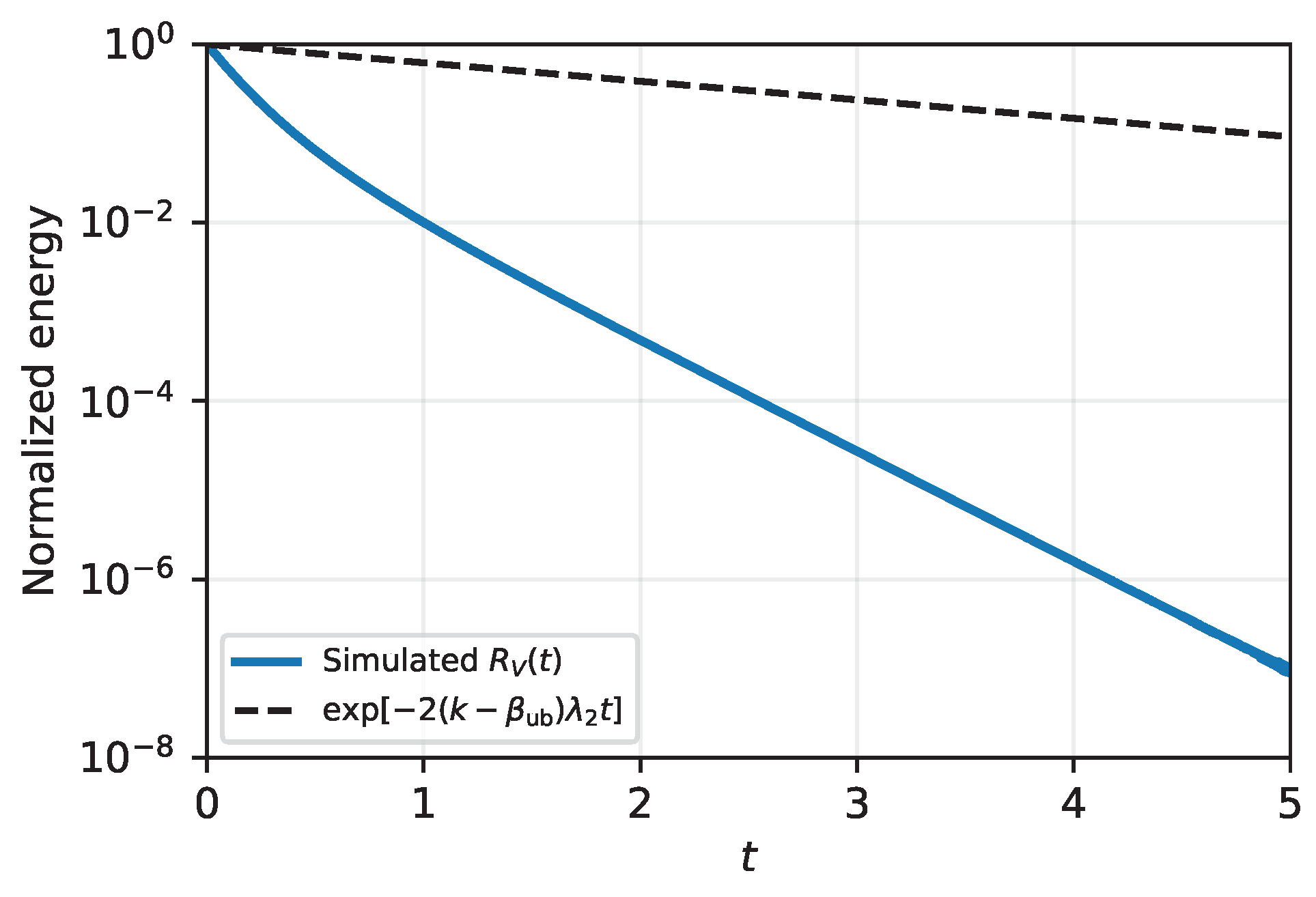
To verify the certified convergence rate in Theorem 1, we used the original five-agent graph and trained controller. We defined the empirical mean normalized Lyapunov energy as

$$R_V\left(t\right):={\displaystyle \frac{1}{N_{\mathrm{test}}}}{\displaystyle \sum _{q=1}^{N_{\mathrm{test}}}}{\displaystyle \frac{V\left(x^{\left(q\right)}\left(t\right)\right)}{V\left(x^{\left(q\right)}\left(0\right)\right)}},V\left(x\right)=\frac{1}{2}{x}^{\top }Lx,$$

where $N_{\mathrm{test}}=200$. Since ${\beta }_{\mathrm{ub}}$ was a valid global gain bound for the residual branch, Theorem 1 could be applied with $\beta ={\beta }_{\mathrm{ub}}$, yielding $R_V\left(t\right)\le \exp [-2(k-{\beta }_{\mathrm{ub}}){\lambda }_{2}t]$. With $k=1.44006$, ${\beta }_{\mathrm{ub}}=1.26715$, and ${\lambda }_2=1.381966$, the certified decay rate was $2(k-{\beta }_{\mathrm{ub}}){\lambda }_2=0.47791$. A logarithmic vertical axis was used to compare the simulated decay with this certified bound.

As shown in Figure 7, the simulated normalized Lyapunov energy $R_V\left(t\right)$ decayed faster than the certified exponential bound. This result indicates that the convergence-rate estimate in Theorem 1 is conservative while still providing a valid upper bound on the observed closed-loop decay.

Figure 7. Verification of the certified convergence rate under the trained controller. The blue curve shows the simulated normalized Lyapunov energy $R_V\left(t\right)$. The black dashed curve shows the certified bound $\exp [-2(k-{\beta }_{\mathrm{ub}}){\lambda }_{2}t]$, where $2(k-{\beta }_{\mathrm{ub}}){\lambda }_2=0.47791$.

6.5. Topology and Network-Size Sensitivity

To examine topology and network-size sensitivity, the controller trained on the original five-agent graph was directly deployed, without retraining or parameter adjustment, on unit-weight ring, star, and complete graphs with $N=5$, 10, and 20. The trained parameters remained $k=1.44006$ and ${\beta }_{\mathrm{ub}}=1.26715$. All controller parameters and evaluation settings, except for the topology and network size, were kept unchanged. For each N, the initial states were sampled independently from the same componentwise distribution specified in Table 1.

For each configuration, Table 4 reports the algebraic connectivity ${\lambda }_2$, the digital-stability margin ${\mu }_h^{\mathrm{ub}}$, the total cost $J_{\mathrm{total}}$, and the terminal normalized Lyapunov energy $R_V\left(T\right)$. The performance indices are reported as mean ± standard deviation over 200 trials.

Table 4. Topology and network-size sensitivity of the trained controller. Results are reported as mean ± standard deviation over 200 trials.

Topology	N	${\mathit{\lambda }}_2$	${\mathit{\mu }}_{\mathit{h}}^{\mathbf{ub}}$	${\mathit{J}}_{\mathbf{total}}$	${\mathit{R}}_{\mathit{V}}\left(\mathit{T}\right)$
Ring	5	1.382	0.1597	$0.422\pm 0.214$	$(2.42\pm 1.90)\times {10}^{-7}$
	10	0.382	0.1583	$0.703\pm 0.319$	$(1.04\pm 1.31)\times {10}^{-3}$
	20	0.09789	0.1583	$1.02\pm 0.437$	$(2.38\pm 2.05)\times {10}^{-3}$
Star	5	1	0.1546	$0.580\pm 0.268$	$(1.62\pm 1.04)\times {10}^{-5}$
	10	1	0.1363	$0.668\pm 0.231$	$(1.97\pm 0.898)\times {10}^{-5}$
	20	1	0.09963	$0.778\pm 0.175$	$(1.98\pm 0.887)\times {10}^{-5}$
Complete	5	5	0.1546	$0.456\pm 0.238$	$(3.83\pm 2.32)\times {10}^{-9}$
	10	10	0.1363	$0.844\pm 0.267$	$(5.62\pm 7.22)\times {10}^{-10}$
	20	20	0.09963	$1.74\pm 0.344$	$(1.37\pm 3.38)\times {10}^{-10}$

Table 4 shows that ${\mu }_h^{\mathrm{ub}}>0$ for all tested configurations. For ring graphs, the total cost and terminal normalized Lyapunov energy increased with N, consistent with the decrease in ${\lambda }_2$. The star graphs yielded similar terminal normalized Lyapunov energies across the tested network sizes. The complete graphs achieved the smallest terminal normalized Lyapunov energies, although their total cost increased with network size. These results demonstrate direct deployment across the tested configurations rather than unrestricted large-scale scalability.

7. Conclusions

This paper proposes a stability-certified ResNN controller for leaderless consensus of first-order multi-agent systems. A computable residual-gain bound yields an exponential-consensus certificate whose rate depends on the gain margin and graph connectivity. A complementary forward-Euler condition guarantees convergent digital implementation.

Spectral projection, gain reparameterization, and digital-margin verification preserve certificate feasibility throughout training. Our numerical results verified the certified decay bound, demonstrated competitive disagreement–effort trade-offs, and showed direct deployment across the tested graph topologies and network sizes.

The current analysis was limited to first-order agents over fixed undirected graphs. Future work will consider more general dynamics, directed or switching graphs, disturbances, delays, and event-triggered communication.

References

- Xu, L.; Su, Y.; Cai, H. Cooperative global K-exponential tracking control of multiple mobile robots. IEEE Trans. Autom. Control 2025, 70, 1214–1221. [Google Scholar] [CrossRef] [Scilit]
- Yu, X.; Su, R. Decentralized circular formation control of nonholonomic mobile robots under a directed sensor graph. IEEE Trans. Autom. Control 2023, 68, 3656–3663. [Google Scholar] [CrossRef] [Scilit]
- Mu, X.; Gu, Z.; Lu, Q. Memory-event-triggered consensus control for multi-UAV systems against deception attacks. ISA Trans. 2023, 139, 95–105. [Google Scholar] [CrossRef] [Scilit] [PubMed]
- Hu, W.; Li, Z.; Dai, M.Z.; Huang, T. Robust adaptive control for spacecraft attitude synchronization subject to external disturbances: A performance adjustable event-triggered mechanism. Int. J. Robust Nonlinear Control 2023, 33, 2392–2408. [Google Scholar] [CrossRef] [Scilit]
- Olfati-Saber, R.; Fax, J.A.; Murray, R.M. Consensus and Cooperation in Networked Multi-Agent Systems. Proc. IEEE 2007, 95, 215–233. [Google Scholar] [CrossRef] [Scilit]
- Ren, W.; Beard, R.W. Consensus Seeking in Multiagent Systems Under Dynamically Changing Interaction Topologies. IEEE Trans. Autom. Control 2005, 50, 655–661. [Google Scholar] [CrossRef] [Scilit]
- Mamoon, M.; Mustafa, G.; Iqbal, N.; Rehan, M.; Ahmed, I.; Khalid, M. An adaptive neural network approach for resilient leader-following consensus control of multi-agent systems under cyber-attacks. ISA Trans. 2025, 157, 20–34. [Google Scholar] [CrossRef] [Scilit] [PubMed]
- Mesbahi, M.; Egerstedt, M. Graph Theoretic Methods in Multiagent Networks; Princeton University Press: Princeton, NJ, USA, 2010. [Google Scholar]
- Xie, K.; Zhao, X.; Chen, S.; Zhang, Z.; Zheng, Y. Distributed optimal consensus of nonlinear multi-agent systems under intermittent communication networks. ISA Trans. 2026, 169, 88–100. [Google Scholar] [CrossRef] [Scilit] [PubMed]
- Zhang, J.; Zhang, H.; Sun, S. Adaptive Dynamic Event-Triggered Bipartite Time-Varying Output Formation Tracking Problem of Heterogeneous Multiagent Systems. IEEE Trans. Syst. Man Cybern. Syst. 2024, 54, 12–22. [Google Scholar] [CrossRef] [Scilit]
- Xiao, L.; Boyd, S. Fast Linear Iterations for Distributed Averaging. Syst. Control Lett. 2004, 53, 65–78. [Google Scholar] [CrossRef] [Scilit]
- Li, Z.; Duan, Z.; Lewis, F.L. Distributed robust consensus control of multi-agent systems with heterogeneous matching uncertainties. Automatica 2014, 50, 883–889. [Google Scholar] [CrossRef] [Scilit]
- Zuo, Z.; Wang, C.; Ding, Z. Robust consensus control of uncertain multi-agent systems with input delay: A model reduction method. Int. J. Robust Nonlinear Control 2017, 27, 1874–1894. [Google Scholar] [CrossRef] [Scilit]
- Borrelli, F.; Keviczky, T. Distributed LQR Design for Identical Dynamically Decoupled Systems. IEEE Trans. Autom. Control 2008, 53, 1901–1912. [Google Scholar] [CrossRef] [Scilit]
- Zhang, H.; Hu, X. Consensus control for linear systems with optimal energy cost. Automatica 2018, 93, 83–91. [Google Scholar] [CrossRef] [Scilit]
- Hu, Z.; Ma, R. Adaptive event-triggered tracking control via switching functions. Automatica 2026, 185, 112813. [Google Scholar] [CrossRef] [Scilit]
- Liu, G.; Liang, H.; Wang, R.; Sui, Z.; Sun, Q. Adaptive Event-Triggered Output Feedback Control for Nonlinear Multiagent Systems Using Output Information Only. IEEE Trans. Syst. Man Cybern. Syst. 2025, 55, 7639–7650. [Google Scholar] [CrossRef] [Scilit]
- Zhang, D.; Meng, L.; Liang, L.; Qin, C.; Liu, D. Dynamic Event-Triggered Control for Human–Machine Cooperative Systems Based on Dynamic Authority Allocation. IEEE Trans. Syst. Man Cybern. Syst. 2026, 56, 3733–3744. [Google Scholar] [CrossRef] [Scilit]
- Levine, S.; Abbeel, P. Learning Neural Network Policies with Guided Policy Search under Unknown Dynamics. In Proceedings of the Advances in Neural Information Processing Systems, Montreal, QC, Canada, 8–13 December 2014; Volume 27, pp. 1071–1079. [Google Scholar]
- Wu, H.; Fan, C.; Zhang, D. An innovative neural network architecture designed for industrial fault diagnosis with hierarchical adaptive attention mechanism. Process Saf. Environ. Prot. 2026, 205, 108162. [Google Scholar] [CrossRef] [Scilit]
- Yin, H.; Seiler, P.; Arcak, M. Stability Analysis Using Quadratic Constraints for Systems with Neural Network Controllers. IEEE Trans. Autom. Control 2022, 67, 1980–1987. [Google Scholar] [CrossRef] [Scilit]
- Fazlyab, M.; Morari, M.; Pappas, G.J. Safety Verification and Robustness Analysis of Neural Networks via Quadratic Constraints and Semidefinite Programming. IEEE Trans. Autom. Control 2022, 67, 1–15. [Google Scholar] [CrossRef] [Scilit]
- García, J.; Fernández, F. A Comprehensive Survey on Safe Reinforcement Learning. J. Mach. Learn. Res. 2015, 16, 1437–1480. [Google Scholar]
- de Souza, C.; Girard, A.; Tarbouriech, S. Event-triggered neural network control using quadratic constraints for perturbed systems. Automatica 2023, 157, 111237. [Google Scholar] [CrossRef] [Scilit]
- Berkenkamp, F.; Turchetta, M.; Schoellig, A.P.; Krause, A. Safe Model-Based Reinforcement Learning with Stability Guarantees. In Proceedings of the Advances in Neural Information Processing Systems, Long Beach, CA, USA, 4–9 December 2017; Volume 30, pp. 908–918. [Google Scholar]
- Chow, Y.; Nachum, O.; Faust, A.; Dueñez-Guzmán, E.; Ghavamzadeh, M. Safe Policy Learning for Continuous Control. In Proceedings of the Conference on Robot Learning; PMLR: New York, NY, USA, 2021; Volume 155, pp. 801–821. [Google Scholar]
- Chang, Y.C.; Roohi, N.; Gao, S. Neural Lyapunov Control. In Proceedings of the Advances in Neural Information Processing Systems, Vancouver, BC, Canada, 8–14 December 2019; Volume 32, pp. 3240–3249. [Google Scholar]
- Megretski, A.; Rantzer, A. System Analysis via Integral Quadratic Constraints. IEEE Trans. Autom. Control 1997, 42, 819–830. [Google Scholar] [CrossRef] [Scilit]
- Gouk, H.; Frank, E.; Pfahringer, B.; Cree, M.J. Regularisation of Neural Networks by Enforcing Lipschitz Continuity. Mach. Learn. 2021, 110, 393–416. [Google Scholar] [CrossRef] [Scilit]
- Tsuzuku, Y.; Sato, I.; Sugiyama, M. Lipschitz-Margin Training: Scalable Certification of Perturbation Invariance for Deep Neural Networks. In Proceedings of the Advances in Neural Information Processing Systems, Montreal, QC, Canada, 2–8 December 2018; Volume 31, pp. 6542–6551. [Google Scholar]
- Miyato, T.; Kataoka, T.; Koyama, M.; Yoshida, Y. Spectral Normalization for Generative Adversarial Networks. In Proceedings of the International Conference on Learning Representations, Vancouver, BC, Canada, 30 April–3 May 2018. [Google Scholar]
- Chen, S.; Cai, S.; Chen, T.; Xu, C.; Chu, J. Neural Observer With Lyapunov Stability Guarantee for Uncertain Nonlinear Systems. IEEE Trans. Neural Netw. Learn. Syst. 2024, 35, 11527–11541. [Google Scholar] [CrossRef] [Scilit] [PubMed]
- He, K.; Zhang, X.; Ren, S.; Sun, J. Deep Residual Learning for Image Recognition. In Proceedings of the IEEE Conference on Computer Vision and Pattern Recognition, Las Vegas, NV, USA, 27–30 June 2016; pp. 770–778. [Google Scholar] [CrossRef] [Scilit]
- Hairer, E.; Nørsett, S.P.; Wanner, G. Solving Ordinary Differential Equations I: Nonstiff Problems, 2nd ed.; Springer: Berlin/Heidelberg, Germany, 1993. [Google Scholar]
- Butcher, J.C. Numerical Methods for Ordinary Differential Equations, 3rd ed.; John Wiley & Sons: Chichester, UK, 2016. [Google Scholar]
- Lowe, R.; Wu, Y.; Tamar, A.; Harb, J.; Abbeel, P.; Mordatch, I. Multi-Agent Actor-Critic for Mixed Cooperative-Competitive Environments. In Proceedings of the Advances in Neural Information Processing Systems, Long Beach, CA, USA, 4–9 December 2017; Volume 30, pp. 6379–6390. [Google Scholar]
Disclaimer/Publisher’s Note: The statements, opinions and data contained in all publications are solely those of the individual author(s) and contributor(s) and not of MDPI and/or the editor(s). MDPI and/or the editor(s) disclaim responsibility for any injury to people or property resulting from any ideas, methods, instructions or products referred to in the content. |
© 2026 by the authors. Licensee MDPI, Basel, Switzerland. This article is an open access article distributed under the terms and conditions of the Creative Commons Attribution (CC BY) license.