1. Introduction
LiDAR as the core sensor for environmental perception and target detection, achieves accurate distance measurement by emitting high-energy pulsed light waves and calculating round-trip time differences, making it indispensable in intelligent perception systems. Compared with traditional radar and optical imaging sensors, it can synchronously collect target distance, angle, and reflection intensity to construct high-precision 3D point cloud models [
1] and can also rely on geometric features to complete target and subcategory classification [
2]. It is widely used in key tasks such as precise target detection [
3,
4,
5], multi-target classification and recognition, and real-time target tracking [
6,
7,
8].
However, due to various factors in complex environments, the target echo signals obtained by its detection exhibit sparsity, which in turn leads to sparsity in the obtained three-dimensional point cloud [
9,
10,
11,
12,
13]. This sparsity can result in the loss of key discriminative features such as geometric structure and local details of the detected target, greatly reducing the overall accuracy of point cloud target classification tasks [
14,
15,
16] and becoming a core bottleneck for improving target perception and decision-making efficiency in complex environments. Therefore, achieving high-precision point cloud target classification under sparse point cloud conditions has key scientific significance and engineering application value for improving target perception and decision-making efficiency in complex environments.
Currently, research in the field of point cloud classification has made certain progress. Researchers have proposed various optimization methods centered around the core issue of sparse point cloud classification, forming different technical paths. Existing sparse point cloud classification methods are mainly divided into two major technical directions, relying on efficient sequence modeling and global dependency modeling capabilities for optimization, respectively. The relevant research progress is as follows:
In terms of efficient sequence modeling, the Mamba model, as an efficient long sequence modeling framework based on the selective state space model (SSM) adopts a linear complexity (O (Nd)) sequence processing mechanism and effectively captures the long-range dependencies of the target through gate state updates and local convolution enhancement strategies, while significantly reducing computational costs, making it a popular research direction for sparse point cloud classification in recent years. However, existing point cloud processing methods based on Mamba still face significant bottlenecks. On the one hand, the one-dimensional sequence modeling paradigm relies on the point cloud serialization strategy, which makes it difficult to fully preserve the local fine geometric structure in three-dimensional space, resulting in the model being unable to effectively mine the key discriminative features of point clouds. On the other hand, existing methods lack effective cross-scale feature aggregation mechanisms when dealing with sparse structures of targets, resulting in insufficient feature representation and discrimination capabilities. Further optimization is needed in sparse point cloud classification scenarios to improve their classification accuracy and robustness [
17,
18,
19,
20,
21,
22].
In terms of global dependency modeling, Transformer utilizes a multi-head attention mechanism to break through the inherent limitations of traditional local modeling paradigms such as convolution and multi-layer perceptron (MLP), effectively capturing the global feature associations of target point clouds, and has become an efficient tool for point cloud global feature learning. However, the computational complexity of its self-attention mechanism is quadratic with the number of points in the point cloud (O(N
2d), where d represents the feature dimension). The high computational and memory costs when dealing with large-scale sparse point clouds make it difficult to meet the real-time requirements of scenarios such as autonomous driving and real-time information processing, severely limiting their practical engineering applications. Although subsequent research has reduced complexity to sub-quadratic levels through optimization strategies such as sparse attention and hierarchical attention, these methods either start by sacrificing global correlation or rely on specific sampling strategies, which limit feature extraction and generalization capabilities. There is still considerable room for improvement in feature representation and classification accuracy for sparse point cloud classification [
23,
24,
25,
26,
27,
28].
In response to the above issues, this paper proposes a sparse point cloud classification method based on the MSE-Mamba neural network. This method achieves high-precision and efficient classification of sparse point clouds by extracting local features at multiple spatial scales and globally integrating high-dimensional features based on attention mechanism, breaking through the technical bottleneck of existing methods. The main tasks and innovative points are as follows:
A multi-scale point cloud adaptive grouping strategy is proposed: The core point set that uniformly covers the point cloud space is filtered through farthest point sampling (FPS), and the basic K-nearest neighbor neighborhood is constructed with the core points as anchors, further generating sub-scale neighborhoods. Combined with neighborhood coordinate centering processing, it effectively eliminates the interference of global position changes of the target, achieving comprehensive capture of sparse structural information such as edge details and local protrusions at different scales, laying a stable and rich foundation for subsequent feature extraction.
A multi-scale feature extraction Mamba module (MSE-Mamba) is constructed: It achieves feature extraction of the target at different scales, and simultaneously enhances the extracted local geometric features by combining KNorm neighborhood adaptive normalization and KPool exponential weighted aggregation mechanism, significantly improving the feature discrimination ability of the overall network model.
A Transformer module based on global attention mechanism (GA-Transformer) is designed: It injects spatial coordinate information into feature representations through learnable positional embeddings and combines multi-head self-attention mechanism to efficiently model long-range semantic associations between core points, thereby enhancing the feature discrimination ability of the overall network model.
2. Principle of Sparse Point Cloud Classification Method Based on MSE-Mamba
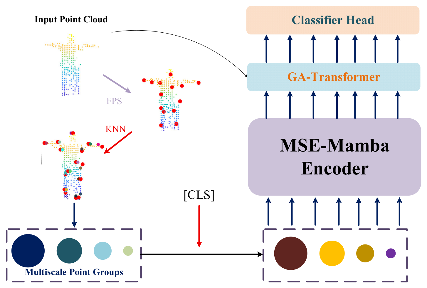
Addressing the issue of feature loss caused by the sparsity of point clouds, which leads to a decrease in classification accuracy, this study proposes a sparse point cloud classification method based on MSE-Mamba. The overall structure of the MSE-Mamba network model is shown in
Figure 1.
The MSE-Mamba network model primarily comprises four modules: FPS and KNN point cloud multi-scale adaptive grouping, MSE-Mamba multi-scale local feature encoding (MSE-Mamba encoder), global feature encoding based on global attention Transformer (GA-Transformer), and classifier output module (classifier head). Through feature extraction and fusion across these modules, high-precision classification of sparse point clouds is ultimately achieved.
2.1. Multi-Scale Adaptive Grouping of Point Clouds
The input sparse point cloud
can be expressed as
, where B represents the batch size, and
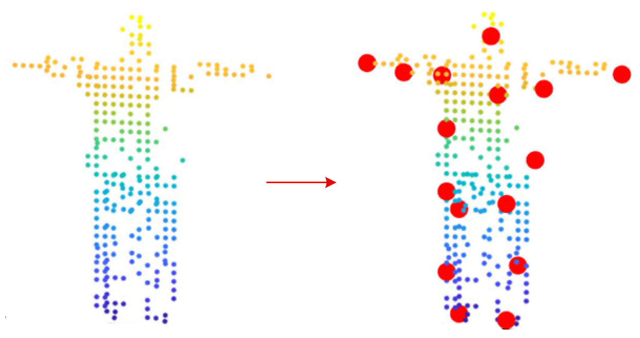
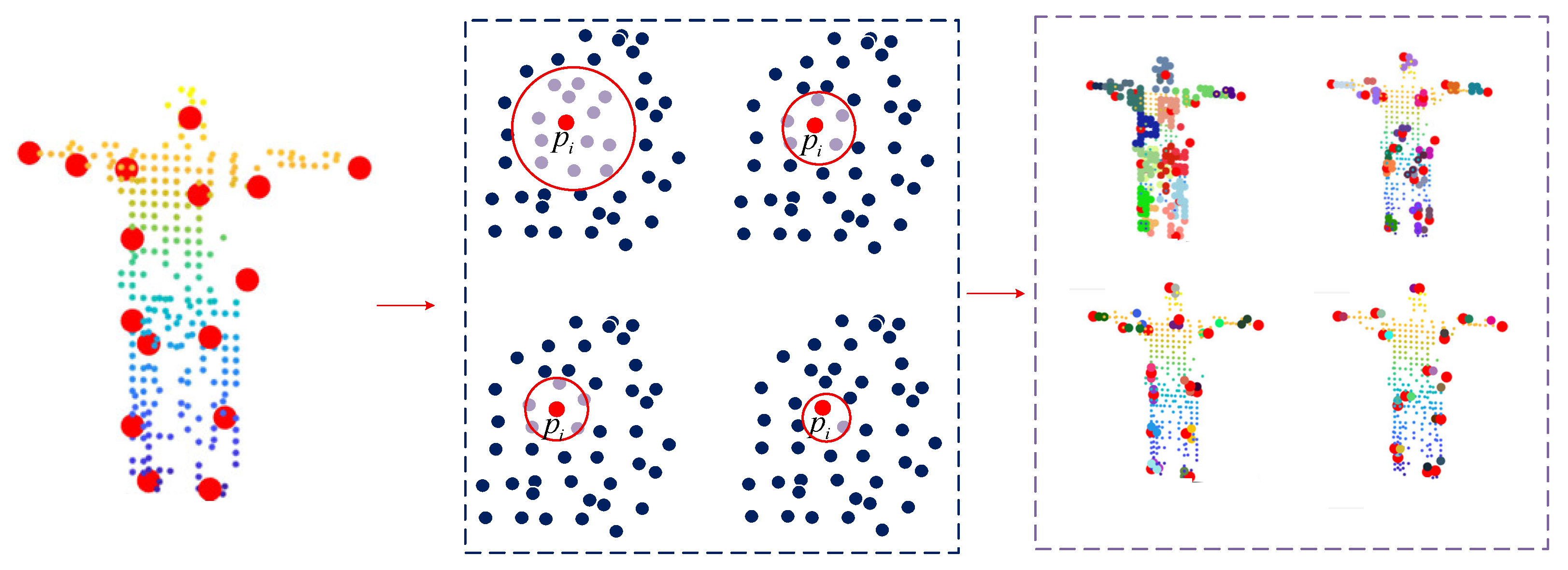
denotes the three-dimensional coordinates of the i-th. To ensure uniform distribution of core points, using the farthest point sampling (FPS) method, G core points are repeatedly sampled to fully cover the point cloud space, providing stable anchor points for subsequent local neighborhood feature extraction, forming a core point set
. The schematic diagram is shown in
Figure 2.
First, randomly select the initial core points
∈
; the selection criteria for the (g + 1)th core point must satisfy the following formula:
Secondly, centered around each core point
, search the original sparse point cloud
for the K nearest points of each core point
to form a local neighborhood
; the global neighborhood set can be represented as
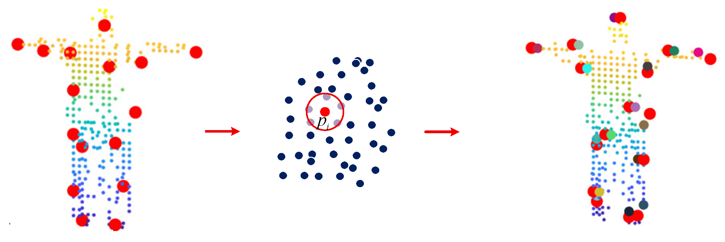
, an example of visualizing the query results of the K-nearest neighbor of the core point is shown in
Figure 3.
To avoid interference from changes in the global position of the target on local feature extraction, the coordinates of the neighboring points in the neighborhood of the core point are centered relative to the core point, , where is the set of core points, is a K-dimensional all-one vector, ⊗ denotes the tensor outer product, and the subscript 0 represents the initial neighborhood of each core point.
To capture target structures of different sizes, in addition to the basic grouping of each core point
, three sub-scale neighborhoods are generated through KNN query to form
, three sub-scale neighborhoods; after extracting features from multiple scales in parallel, they are fused to comprehensively capture sparse structural information at different scales, such as edge details and local protrusions. The visualization diagram of multi-scale regional division is shown in
Figure 4 and this can be expressed as:
2.2. MSE-Mamba Multi-Scale Local Feature Encoding
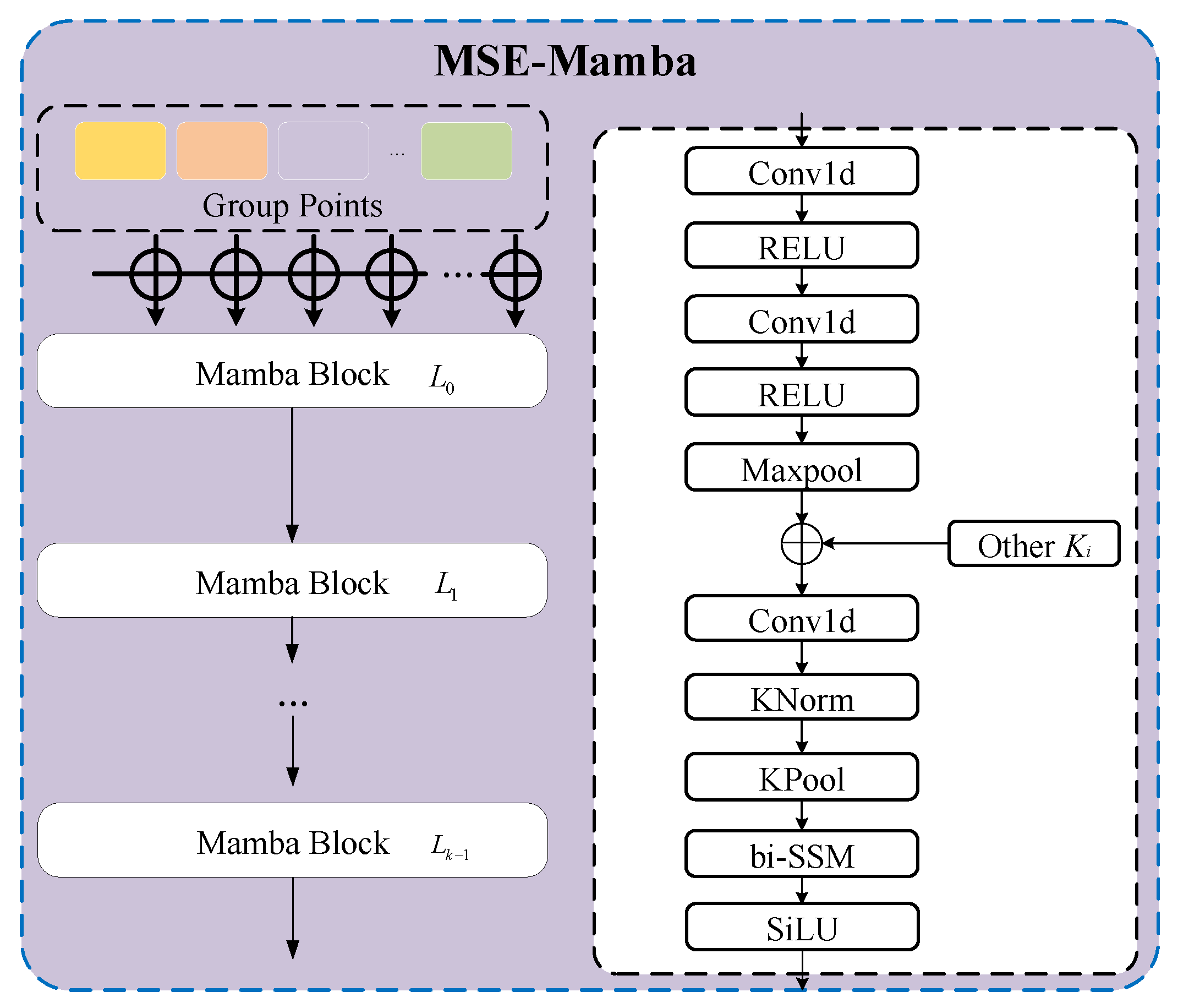
The MSE-Mamba feature encoding module achieves precise capture of multi-scale local geometric features through lightweight operations, while maintaining the advantage of linear complexity. Its structure is shown in
Figure 5 below.
For all points within each scale neighborhood
, to lay the groundwork for subsequent feature extraction and computation, we first perform dimensionality transposition, converting the 3D coordinates into the channel dimension of convolution. The transposed results for the four scale neighborhoods are represented as follows:
After transposing the dimensions, it is passed through two layers of 1D convolution and RELU activation function to map the 3D coordinates to high-dimensional features. The first layer increases the dimension to 128, and the second layer increases it to 256:
And we extract global structural features through global max pooling:
After extracting the global structural features of each neighborhood, the global structural features are expanded to match the dimensionality of the local feature points, ensuring that the features of each neighborhood point encompass both its own local details and the global structural information of the entire neighborhood. This achieves a deep fusion of local and global semantics:
We perform the same operation as described above for all points within each scale neighborhood Ki to obtain
. Then, we concatenate the
from each neighborhood and apply one-dimensional convolution:
At this time, the following issues are also faced: The core point neighborhood of the target edge is usually sparse and has a large distribution range, while the core point neighborhood of the target center is usually dense and has a small distribution range. This uneven density makes the local features of different core points vary greatly in amplitude and variance, further exacerbating the fluctuation of feature distribution after fusion. To address this, this paper eliminates the scale bias of sparse point clouds through neighborhood adaptive normalization of KNorm, and simultaneously utilizes KPool exponential weighted aggregation to strengthen key features while retaining structural information, thereby enhancing the overall feature discrimination ability of the network model and laying a solid foundation for subsequent global feature learning:
where
,
is a learnable parameter and Norm(⋅) denotes a normalization operation. The weights for weighted pooling are generated by the feature itself through an exponential function
, with no additional learnable parameters. The weights are adaptively allocated solely through the exponential mapping of feature values, aiming to assign higher weights to key local structures with larger feature values.
To eliminate the dependency of a single point cloud sequence in the feature extraction process, this paper employs bidirectional state space modeling (bi-SSM) to perform forward and backward state space modeling on
, respectively. This enables the overall network model to more fully capture the local contextual information of the target, extract more comprehensive local geometric features from the target point cloud, and enhance the discriminative power and robustness of the network model towards features. By fusing the bidirectional modeling results with the original features, an enhanced feature
is outputted:
Finally, we perform layer normalization on the bidirectional fused features and enhance nonlinear expression through SiLU activation:
So far, multi-scale local feature extraction has been completed through MSE-Mamba feature encoding. Next, we aim to address the limitations of local modeling.
2.3. Global Feature Encoding Based on Global Attention Transformer
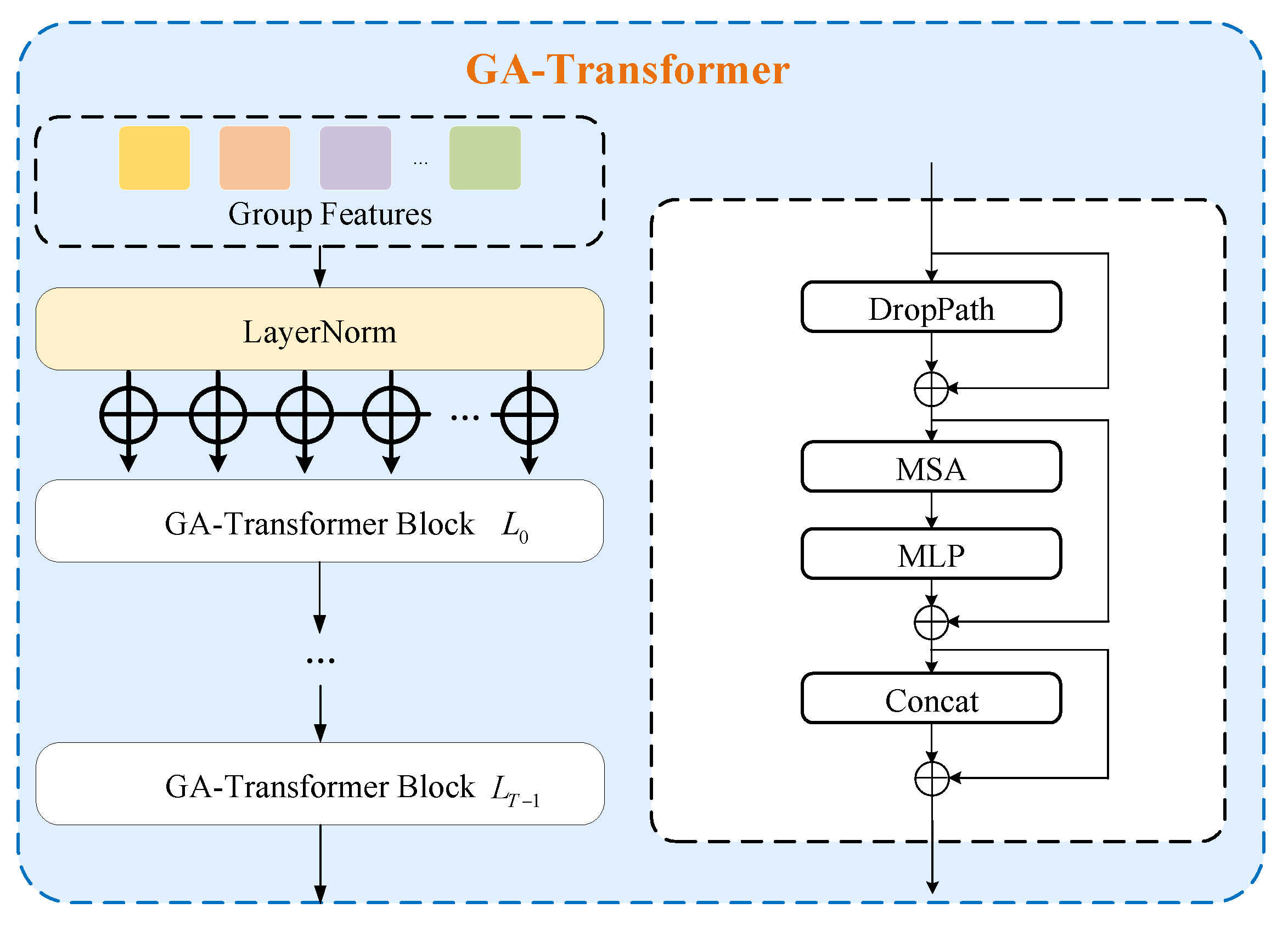
Single local enhancement lacks global dependency modeling between core points (such as the semantic association of core points in different parts of the target), while the multi-head self-attention mechanism of Transformer excels at capturing global interactions. It ensures training stability through residual connections and layer normalization, achieving synergistic enhancement of local structure and global dependencies. The structure of the GA Transformer global feature extraction module mentioned in this article is shown in
Figure 6.
For
with local feature modeling completed, the DropPath random dropout strategy is introduced to prevent overfitting, and the original features are fully retained through residual connections to avoid the loss of useful information during the enhancement process, providing high-quality local feature support for global modeling:
Secondly, through multi-head self-attention computation,
is converted into Q, K
GA-Transformer, and V vectors. At the same time, global correlation is calculated through dot product attention, and a scaling factor
is introduced to balance the scale and avoid excessively large attention values:
where W
Q, W
K and W
V are attention weight matrices, and H represents the number of attention heads.
After enhancing
through MLP, we perform a residual connection with the initial global feature
to further enhance the network model’s ability to express the target global features:
Before that, the 3D coordinate
of the core point is expanded to the same dimension D as the global features through an MLP to obtain
. Additionally, a learnable position embedding
, which is continuously optimized during training, is specifically added during model initialization. The two are fused to obtain a complete set of position embeddings
in order to enable the classification token to also carry position information and maintain consistency with other core point features:
Finally, the complete position embedding is directly added to the global enhanced features, allowing each global feature to carry corresponding spatial coordinate information:
The features outputted in this way encompass both the semantic information and spatial position information of the point cloud, providing a more precise basis for subsequent classification tasks.
2.4. Category Output Module(Classifier Head)
After local and global feature extraction and integration, the semantic information and spatial position information
containing point clouds are finally fed into the classification head to complete the probability calculation of the target category. In order to fully utilize this information to improve classification accuracy, this paper adopts a multi-feature aggregation strategy to generate the final global feature vector of the target, which consists of three parts: the feature vector
corresponding to the category label, the feature vector
obtained by max-pooling
and the feature vector
obtained by average-pooling
. These vectors are mapped to the target category space through a linear layer, and the probability of each category is calculated using the
function to complete the classification prediction. The formula is as follows:
In this context, represents a multi-layer perceptron used for category prediction, which calculates probabilities using Softmax to obtain the final category probability distribution . C denotes the number of categories. During the training phase, cross-entropy loss is employed to optimize the model parameters, while during the inference phase, the category with the highest probability is selected as the final prediction result.
3. Results
In order to comprehensively verify the performance and advantages of the proposed method in point cloud classification tasks, this section validates the effectiveness, generalization ability, and robust classification ability of MSE-Mamba on the ModelNet40 dataset [
29], ScanObjectNN dataset [
30], and self-made 3D imaging LiDAR point cloud dataset, respectively. At the same time, multiple mainstream methods based on different backbone networks are selected for comparative experiments. Finally, through detailed ablation experiments, the contribution of each module to the overall performance is analyzed to verify the rationality of the design. Firstly, we introduce the experimental setup, including network configuration, training strategy, and evaluation metrics.
3.1. Experimental Setup and Evaluation Criteria
This study is based on the PyTorch 2.1.0 framework and uses NVIDIA RTX 4070Ti Super graphics card to complete model training. The model embedding dimension is set to 384, the network depth is 4 layers, the number of multi-head attention heads is 6, and the classification output dimension is adaptively adjusted according to the number of categories in the dataset. We training a uniform fixed random seed of 42 to ensure reproducibility of the experiment, with a total of 200 training epochs. After each round of training, the accuracy of OA is evaluated on the validation set, and only the model checkpoints with the best accuracy on the validation set are saved for final testing. We apply unified configuration for data augmentation: we perform 0.95–1.05 times random scaling and ± 0.05 range random translation on point clouds and add [−180°, 180°] global random rotation to ScanObjectNN. The training uses the AdamW [
31] optimizer, with an initial learning rate of 5 × 10
−4 and a weight decay coefficient of 0.05. The learning rate scheduling adopts a cosine annealing strategy with hot restart [
32], with an initial cycle of 200 rounds, a cycle doubling coefficient of 1.8, a minimum learning rate of 1 × 10
−6, and 20 warm-up rounds; we use a batch size of 32 and a gradient clipping threshold of 10. The loss function adopts a cross entropy loss with a label smoothing coefficient of 0.2, and a DropPath probability of 0.2 is used for regularization [
33]. The MLP layer has a dimension expansion coefficient of 4.0, the classification output module Dropout is set to 0.5, and the feature concatenation dimension is 768 (384 × 2). P(M) in all tables in the text represents the number of model parameters, measured in millions (M); F(G) represents the floating-point computational complexity of model inference, measured in GFlops(G).
In order to measure the classification performance of the model, this article uses overall accuracy (OA) as the evaluation metric. Overall accuracy is the most commonly used evaluation metric in point cloud classification tasks, defined as the proportion of correctly classified samples to the total number of samples [
34]:
In the formula, TP (true positive) represents the number of samples that are actually positive and correctly predicted as positive, TN (true negative) represents the number of samples that are actually negative and correctly predicted as negative, and FP (false positive) represents the number of samples that are actually negative and incorrectly predicted as positive, FN (false negative) represents the number of samples that are actually positive but incorrectly predicted as negative.
3.2. Ablation Experiment and Result Analysis
Before discussing other characteristics of the method proposed in this article, it is necessary to conduct a thorough analysis of the contributions of each component in the proposed method and the rationality of the experimental parameter settings. Therefore, this chapter designs a comprehensive ablation experiment, mainly divided into modular ablation experiments and parameter setting ablation experiments, to quantitatively verify and analyze the effectiveness of the components and the rationality of the parameters.
3.2.1. Parameter Settings for Ablation Experiment
To verify the scientificity and rationality of the key parameter settings in the MSE-Mamba network model, multiple ablation experiments were designed for the core parameter scale hierarchy (D, D/2, D/4, D/8) and anchor number (K
a = 8, 16, 32). The impact of different parameter combinations on the model classification performance was systematically analyzed. The experimental results are shown in
Table 1.
The experimental results of scale-level configuration show that multi-scale feature fusion is the key factor to improve the classification performance of the model. When only a single scale (only D) is used, the overall accuracy (OA) of the model is only 92.4%~93.1%, and the performance is relatively limited. With the increase in the number of fusion scales, the classification accuracy gradually improved: When using two scales (D, D/2), the OA increased to 92.5~93.5%. After the integration of three scales (D, D/2, D/4), OA further increased to 92.8~94.0%. When four scale fusion (D, D/2, D/4, D/8) is used, the model achieves the optimal performance, and the highest OA is 94.2%. This result fully proves that multi-scale feature aggregation can comprehensively capture the fine-grained edge details of point clouds at small scales and the global shape contour information at large scales, effectively solving the limitation that a single-scale method is difficult to adapt to different size targets and sparse distribution and achieving richer and more discriminative feature representation.
The experimental results of the number of anchor points (Ka) show that Ka = 16 is the best choice to take into account the performance and computational efficiency of the model. For all scale configurations, when Ka increases from 8 to 16, the model OA is significantly improved: Taking the four scale fusion as an example, when Ka = 8, the OA is 93.2%, when Ka = 16, it is 94.2%, an increase of 1 percentage point. When Ka is further increased to 32, the performance improvement tends to be flat, and the OA remains at 94.2%. This phenomenon shows that when the number of anchor points is insufficient (Ka = 8), the coverage of the whole point cloud space by the core points is not sufficient, resulting in incomplete local neighborhood feature extraction and being unable to fully capture the key structure information of the point cloud. However, when the number of anchor points is too large (Ka = 32), although the spatial coverage can be increased, redundant calculation will be introduced, resulting in an increase in the complexity of the model, and no additional improvement in feature discrimination. Therefore, in this paper, Ka = 16 is set in the specific experiment process, which not only ensures that the core points can fully cover the key areas of the point cloud, and provides stable support for the local feature extraction of the MSE-Mamba module and the long-range correlation feature capture of the GA-Transformer module, but also avoids the computational efficiency reduction caused by excessive anchor points and achieves the best balance between performance and efficiency.
3.2.2. Modular Ablation Experiment
The ablation analysis of the MSE-Mamba and GA-Transformer modules proposed in this paper is carried out through the three-dimensional imaging dataset to verify their effectiveness. By comparing the performance differences of the modules, its role in improving the classification accuracy is evaluated.
See
Table 2 for the effectiveness verification experiment results of each module. From the ablation experiment results, it can be seen that the proposed MSE-Mamba feature coding module and GA-Transformer bring obvious performance gains and make significant contributions to the overall point cloud classification performance of the network. The complete hybrid architecture of MSE-Mamba and GA-Transformer (Variant 1) achieves the highest overall accuracy of 96.82% on the self-built 3D imaging LiDAR dataset with linear computational complexity O(Nd), four-scale adaptive FPS-KNN grouping, and KNorm and KPool sparse feature enhancement mechanisms. When the GA-Transformer module is removed (Variant 2), the model degenerates into a pure Mamba structure similar to Mamba3D without global long-range semantic dependency modeling, resulting in a 0.57% drop in classification accuracy. If the MSE-Mamba multi-scale local feature encoding module is eliminated (Variant 3), the model only relies on simple single-scale grouping for global attention calculation, which has the same limitation of insufficient multi-scale geometric feature mining as PCT, and the overall accuracy decreases by 0.81%. The comparison of three variants fully proves that the joint combination of multi-scale local feature extraction branch and lightweight global attention branch can simultaneously compensate for the inherent defects of pure Mamba architectures lacking global correlation modeling and pure Transformer architectures with weak sparse local feature extraction, achieving better classification performance under linear computational overhead.
3.3. Experiment and Result Analysis of Point Cloud Classification Ability
After the ablation experiment, all baseline models such as PointNet, PCT, PCM and Mamba3D are reimplemented and retrained on the same NVIDIA RTX 4070Ti Super graphics card with identical training hyperparameters and data augmentation strategies. Under the experimental settings of 16 anchor points and 8 scale D, this paper further discusses the sparse point cloud classification performance of MSE-Mamba on ModelNet40, ScanObjectNN and self-made 3D imaging LiDAR point cloud datasets.
3.3.1. Experiment and Result Analysis on the Effectiveness of Point Cloud Classification
The ModelNet40 dataset spans 40 target categories and is an ideal test dataset for verifying the basic performance of the point cloud classification algorithm. The visualization effect is shown in the following
Figure 7. In the specific experimental process, the number of training samples was 9843 frames, and the number of test samples was 2468 frames.
N = 1024 points were used as input, and 0.95 times of random scaling and translation were applied for data enhancement.
The results in
Table 3 show the superiority of MSE-Mamba over the current mainstream point cloud classification methods in the modelnet40 dataset. From the perspective of classification accuracy, MSE-Mamba achieved 94.2% of OA (overall accuracy), showing obvious advantages over the existing methods. Compared with traditional methods that rely on local feature aggregation, such as Pointnet++and DGCNN, MSE-Mamba, with its multi-scale local feature extraction and global modeling capabilities, can more effectively capture the long-distance dependence of point clouds so as to improve the overall accuracy.
Compared with Transformer-based methods (such as PCT), MSE-Mamba not only achieves better classification performance but also avoids the secondary computational complexity inherent in the self-attention mechanism. This gives MSE-Mamba a higher computational efficiency while maintaining high accuracy, and it is suitable for training and testing tasks in large-scale point cloud scenarios.
From the computational complexity and parameter quantity in the experimental results, compared with other Mamba architectures, MSE-Mamba has increased by 0.86% compared with PCM, and the parameter quantity has decreased from 34.2 m to 16.9 m. This significant efficiency improvement is mainly due to the linear computational complexity of Mamba.
3.3.2. Robustness Experiment and Result Analysis of Point Cloud Classification
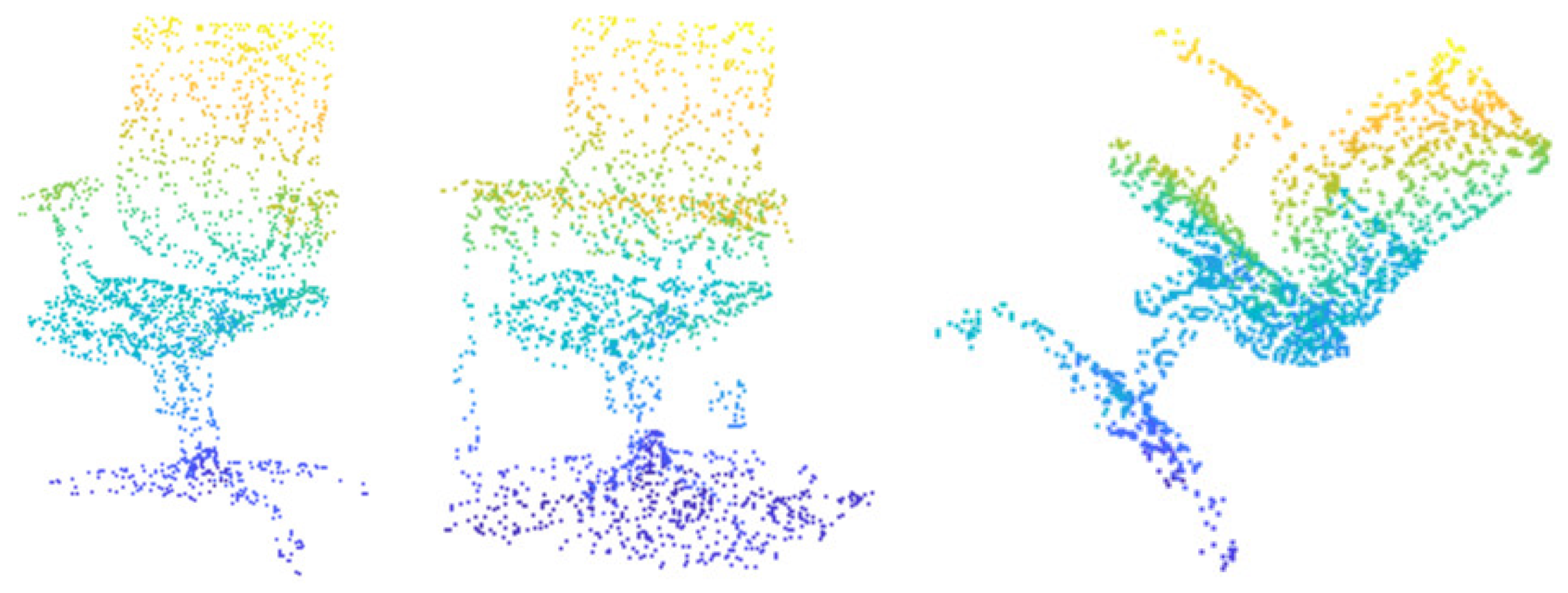
In this study, experiments were conducted using three variant subsets of the ScanObjectNN dataset: OBJ_BG, OBJ_ONLY and PB_T50_RS. The objective is to validate the comprehensive performance superiority of the proposed MSE-Mamba method across multiple dimensions and scenarios and to comprehensively underscore the advantages of our method in handling complex real-world point cloud data by testing it under various feature conditions. The OBJ_ONLY subset comprises pure object point clouds without any background, enabling verification of MSE-Mamba’s feature extraction and representation capabilities for clean point clouds. The OBJ_BG subset includes point cloud data with cluttered backgrounds, allowing assessment of the method’s ability to perform feature selection and mine target information amidst background interference. The PBT_50_RS subset exhibits complex characteristics involving rotation and scaling (random rotation and scaling by 75%). These three variant subsets, each with distinct characteristics, collectively and progressively validate the robustness of the MSE-Mamba method in feature extraction compared to existing methods, ensuring the comprehensiveness and persuasiveness of our experimental validation. The visualization effect is depicted in the following
Figure 8.
During the experiment, the number of training samples for OBJ_BG and OBJ_ONLY was set to 2309 frames, with 581 frames for testing. For PBT_50_RS, the number of training samples was 11,416 frames, and the number of test samples was 2882 frames. During the training process, apart from the input point cloud size N = 2048, which differed from that in ModelNet40, all other strategies remained consistent.
As evidenced by the experimental results presented in
Table 4, the proposed MSE-Mamba network model demonstrates exceptional classification performance and a robust competitive edge, achieving optimal results across all three subsets. This outstanding performance can be primarily attributed to the following factors: Firstly, in contrast to traditional MLP backbone network approaches, the long-sequence modeling capability of MSE-Mamba, grounded in the Mamba architecture, enables it to more effectively capture global dependencies within point clouds, particularly exhibiting enhanced robustness when confronted with complex backgrounds and noise interference. Secondly, when compared to other Transformer-based methods, MSE-Mamba more efficiently processes the local geometric structures of point clouds through its multi-scale point cloud local feature extraction module, a critical advantage when dealing with irregular sampling and local omissions in real-world scanned data. Finally, even in comparison with PCM and Mamba3D, which are also based on the Mamba architecture, MSE-Mamba still exhibits superior performance, thereby fully validating the effectiveness of the proposed strategy for multi-scale local feature extraction and self-attention-based global feature integration.
3.3.3. Validation Experiment and Result Analysis of Point Cloud Classification Under Subsampling Conditions
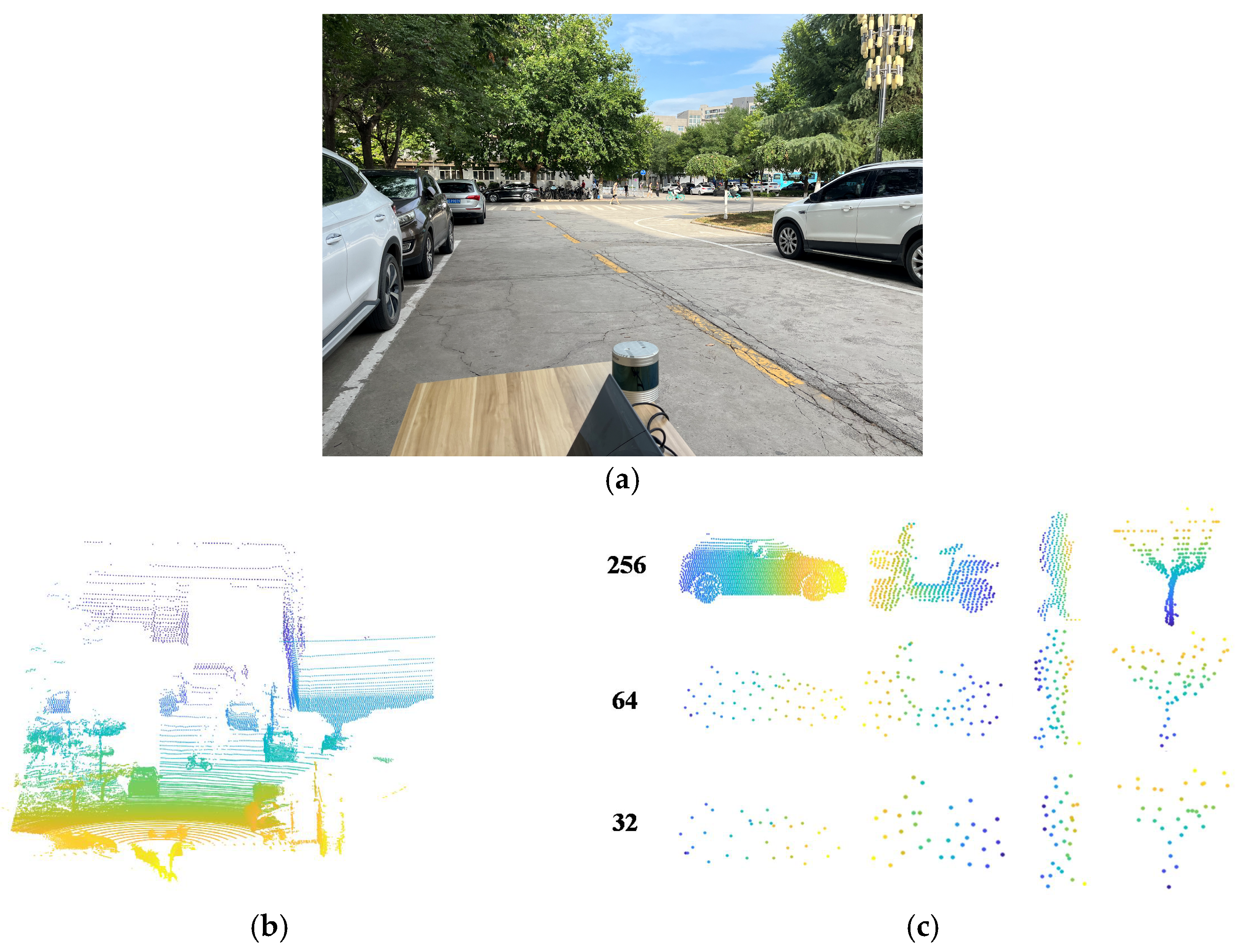
In order to comprehensively verify the classification performance and robustness of the proposed MSE-Mamba network model in real scenes and sparse conditions, this experiment is based on the self-made 3D Imaging LiDAR point cloud dataset. This experiment uses a real scene point cloud dataset collected by the research group based on the Ruby Plus 128 line mechanical LiDAR. The core parameters of the equipment are: laser wavelength of 905 nm, ranging range of 0.3–120 m, ranging accuracy of ± 3 cm, horizontal field of view of 120°, vertical field of view of 32°, frame rate of 10 Hz, synchronized output of three-dimensional coordinates and echo intensity. The dataset adopts a semi-automatic annotation process, which first clusters and roughly divides target instances, and then manually corrects occlusion and boundary misclassification points, uniformly annotating semantic labels for four categories: bicycles, cars, pedestrians, and trees. It collects scenes covering complex working conditions such as local occlusion, strong/weak light, and varying distances. The dataset consists of 1517 valid samples, which are divided into a training set of 1200 frames and a testing set of 317 frames in a 7:3 ratio. Each frame is uniformly downsampled to 256 input points into the network. Due to intellectual property limitations of the project, this self-built dataset is temporarily not publicly available. Researchers can contact the corresponding author via email to apply for improvement of the dataset. The data collection scenario is shown in
Figure 9a, and the collection results are shown in
Figure 9b. The experimental results are shown in
Table 5 and
Table 6.
The real scene dataset contains four categories. These point clouds are real object point clouds scanned in different actual scenes. During the experiment, the collected data were enhanced, including random translation, rotation and scaling disturbance. The number of training samples is 1200 frames, and the number of test samples is 317 frames. Set the input point cloud size N = 256 to compare and analyze the actual classification effect of various methods.
The experimental results of classification on the real-world scene dataset are presented in
Table 5. MSE-Mamba achieved an overall accuracy of 96.82%, significantly outperforming various mainstream comparative methods and fully demonstrating its strong adaptability to diverse targets in real-world scenarios. Specifically, it improved by 2.0 percentage points compared to the traditional PointNet++ (94.83%), which is based on an MLP backbone network, surpassed PCT (95.97%), which is based on a Transformer architecture, by 0.85 percentage points, and also outperformed Mamba3D (96.55%), another model in the Mamba series, by 0.27 percentage points. The core reason for this outstanding performance lies in MSE-Mamba’s multi-scale point cloud adaptive grouping strategy, which can accurately capture the local geometric details and overall structural features of sparse point clouds. Additionally, the synergy between KNorm neighborhood adaptive normalization and KPool index-weighted aggregation mechanisms contributes to this success. Meanwhile, the GA-Transformer module efficiently models long-range semantic associations between core points through learnable positional embeddings and a multi-head self-attention mechanism, breaking through the limitations of traditional local modeling paradigms.
In addition, the point cloud classification ability test experiment with 64 and 32 sampling points under the point cloud is set up. The experimental results are shown in the table below.
The performance advantage of MSE-Mamba is more prominent under the condition of subsampling, which fully reflects its strong robustness to sparse point clouds. When the number of input points is reduced to n = 64, the OA of the model still reaches 92.7%. Even in the sparse scene of n = 32, the model still maintains a high accuracy of 92.1%. This result fully verifies the effectiveness of the MSE-Mamba core module. The model can still extract stable and effective discriminant features in the case of a large number of point clouds missing and complete the task of high-precision classification of point clouds.
3.3.4. Verification Experiment and Analysis of the Robustness of Point Cloud Classification Under Downsampling Conditions
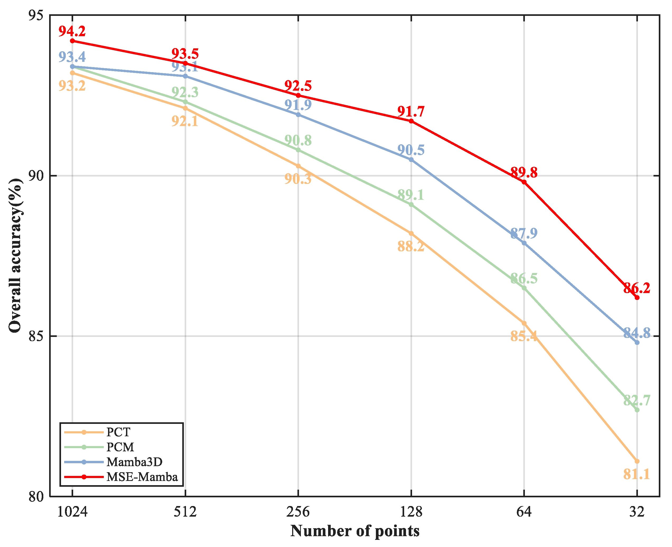
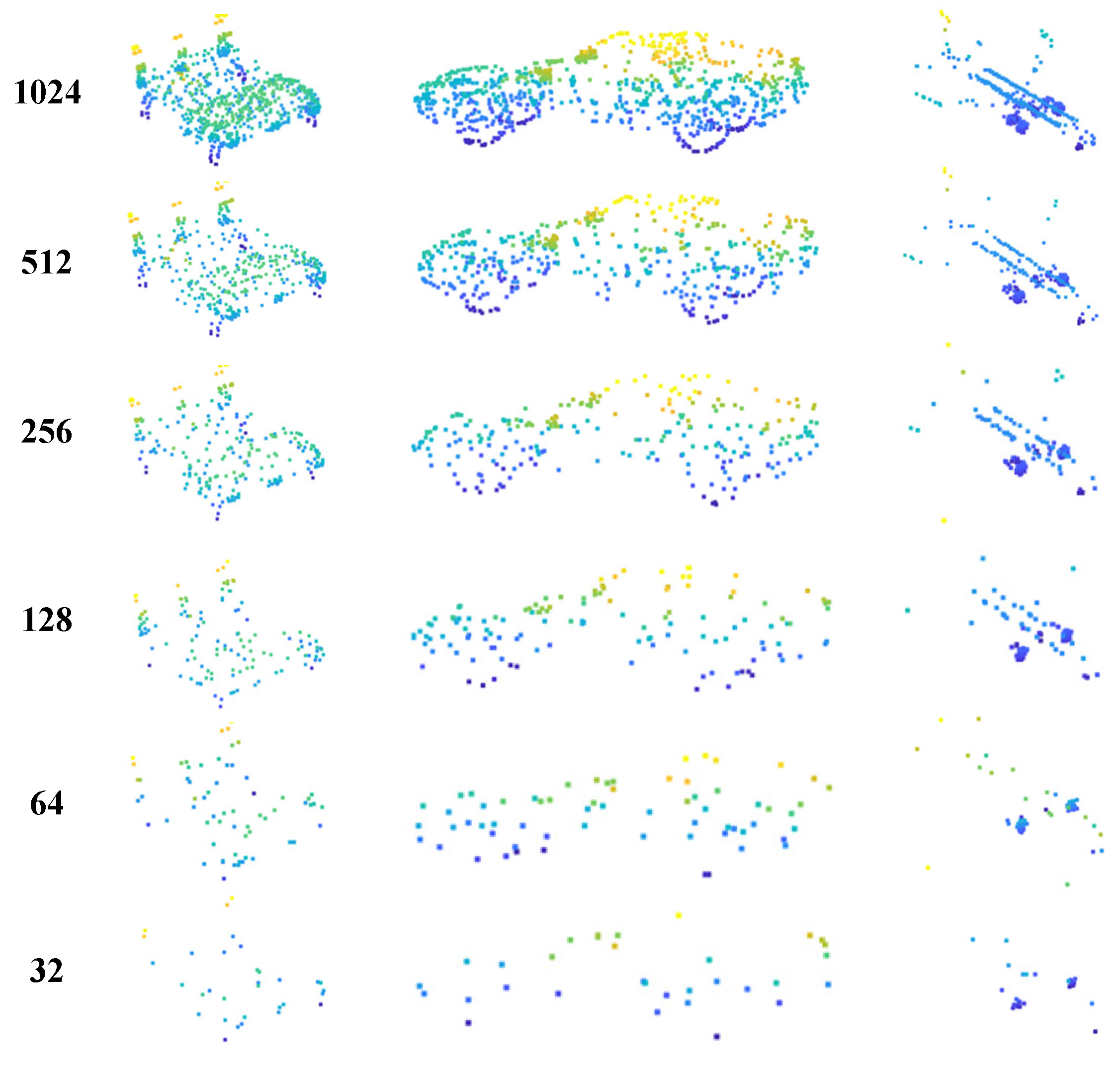
In addition, we conducted experiments on the classification ability of various methods under different sparsity levels (number of points n from 1024 to 32) through the ModelNet40 dataset, in order to explore the robustness of the classification ability of different methods in the gradual decline of the number of point clouds.
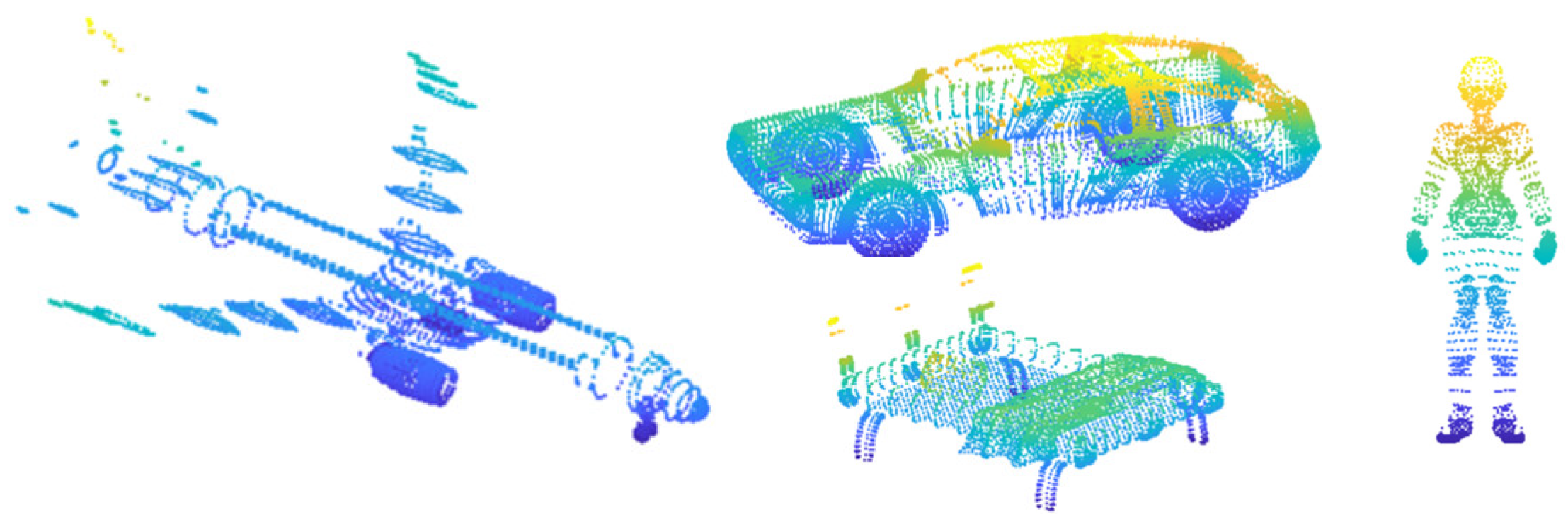
Figure 10 shows the visualization results under different sparsity levels, and
Figure 11 shows the experimental results.
Based on the sparsity verification experiment of gradually sampling the number of point clouds from 1024 to 32 in the ModelNet40 dataset, the system compares the classification robustness of various mainstream methods in the scenario where the sparseness of the point cloud continues to increase. Although the PCT method based on the Transformer architecture realizes the capture of global feature associations in point clouds with the help of the multi-head self-attention mechanism, and the classification performance is better at medium sparseness, the effectiveness of global feature modeling decreases rapidly when the number of point cloud points continues to decrease and the feature information is greatly reduced, and the attenuation trend of classification accuracy gradually accelerates. It is difficult to maintain stable performance in extremely sparse scenarios. However, due to the lack of multi-scale feature aggregation and global semantic association co-optimization design, the effective discriminant features in the remaining point clouds cannot be fully exploited under the condition of sparse point clouds where the number of point clouds drops to 32, and the classification performance is significantly reduced.
In stark contrast, the MSE-Mamba model maintains the lowest accuracy decay rate among all comparison methods during the entire point cloud sampling test, and can still maintain a much higher classification accuracy than other methods even under the sparse condition of only 32 point cloud points, showing strong sparse point cloud classification robustness. The core is that MSE-Mamba realizes the integration of multi-scale local feature extraction and global semantic association modeling, and its multi-scale point cloud adaptive grouping strategy combines KNorm neighborhood adaptive normalization and the KPool exponential weighted aggregation mechanism, which can accurately capture fine-grained edge details and key structural features in the remaining point cloud when a large number of point clouds are missing and feature information is insufficient, effectively making up for the missing features of sparse point clouds and retaining core discriminant information for classification tasks. At the same time, the GA-Transformer global feature coding module integrates spatial coordinate information into the feature representation through learnable position embedding and combines the long-range semantic association between core points to efficiently model the multi-head self-attention mechanism, breaking through the limitations of a single local modeling paradigm, allowing the model to mine more effective discriminant information through global correlation and improve the stability of classification.
In summary, the MSE-Mamba network model shows excellent classification stability, generalization ability and robustness under the sparse conditions of sampling at different degrees in real complex scenarios and under different degrees, which effectively solves the problem of degradation accuracy caused by missing features in sparse point cloud classification.
4. Conclusions
As the core task of LiDAR data processing, point cloud classification directly determines the accuracy and reliability of downstream applications, and existing methods generally have problems such as insufficient local feature capture and low efficiency of global correlation modeling when dealing with sparse point clouds, resulting in a significant decrease in classification accuracy. In order to solve this core problem, a sparse point cloud classification method based on MSE-Mamba is proposed, which realizes the association between local geometric features and global semantic coding through multi-scale point cloud adaptive grouping, MSE-Mamba multi-scale local feature coding and GA-Transformer global feature coding and completes the high-precision classification of sparse point clouds.
The effectiveness, generalization ability and robustness of the proposed method are systematically verified on the ModelNet40, ScanObjectNN and self-made 3D imaging LiDAR datasets. Experimental results show that MSE-Mamba achieves an overall classification accuracy of 94.2% on the ModelNet40 dataset, and the number of parameters is optimized to 16.9M, which is significantly better than the traditional method and the same architecture method, and achieves both accuracy and computational efficiency. It achieves excellent performance on the ScanObjectNN dataset and the subset of variants with background interference and rotational transformation, showing strong classification generalization ability. The overall classification accuracy of the self-made dataset including bicycles, cars, pedestrians and trees is 96.82%, which proves that the proposed method has good adaptability to multi-category targets in real scenarios. For different degrees of downsampling sparse scenes, the proposed method shows outstanding anti-sparsity ability: the classification accuracy is still maintained at 92.1% under the sparse condition of 32 points, and the overall accuracy decay rate is also shown in the downsampling point cloud classification experiment of ModelNet40 dataset from 1024 to 32, which proves that it can still accurately mine core discriminant features under sparse point cloud conditions and achieve high-precision point cloud classification.
In summary, the proposed method provides high-precision and high robustness technical support for sparse point cloud classification, which not only breaks through the limitations of traditional methods in sparse point cloud processing, but also promotes the practical application of LiDAR technology in complex scenarios.
Author Contributions
Conceptualization, G.X.; methodology, G.X.; software, X.L. and B.X.; validation, X.W. and B.X.; writing—original draft preparation, G.X. and C.W.; writing—review and editing, C.W. All authors have read and agreed to the published version of the manuscript.
Funding
This research received no external funding.
Data Availability Statement
Data underlying the results presented in this paper are not publicly available at this time but may be obtained from the authors upon reasonable request.
Acknowledgments
The manuscript was supported by the Xi’an Key Laboratory of Active Photoelectric Imaging Detection Technology.
Conflicts of Interest
The authors declare no conflicts of interest.
References
- El-Diasty, M.; Al-Hashim, A.; Abdalla, R. UAV-Based LiDAR System for Urban Mapping and Modelling Applications. Int. Arch. Photogramm. Remote Sens. Spat. Inf. Sci. 2025, 48, 13–17. [Google Scholar] [CrossRef]
- Jeong, S.; Shin, H.; Kim, M.J.; Kang, D.; Lee, S.; Oh, S. Enhancing LiDAR Mapping with YOLO-Based Potential Dynamic Object Removal in Autonomous Driving. Sensors 2024, 24, 7578. [Google Scholar] [CrossRef] [PubMed]
- Cui, Y.; Li, Z.; Fang, Z. Dynamic Clustering Transformer for LiDAR-based 3D Object Detection. Pattern Recognit. 2025, 157, 110869. [Google Scholar]
- Chen, X.Z.; Chiu, Y.K.; Huang, C.S.; Chen, Y.L. MonoTDF: Temporal Deep Feature Learning for Generalizable Monocular 3D Object Detection. Pattern Recognit. 2026, 176, 113184. [Google Scholar] [CrossRef]
- Liu, Q.; Zhao, D.; Dong, Y.; Xiao, L.; Wang, J.; Min, C.; Li, F.; Jiang, W.; Lu, D.; Nie, Y. PointSlice: Accurate and Efficient Slice-Based Representation for 3D Object Detection from Point Clouds. Pattern Recognit. 2026, 178, 113449. [Google Scholar] [CrossRef]
- Vora, S.; Beijbom, O.O.; Lang, A.H.; Helou, B. Sequential Fusion for 3D Object Detection. U.S. Patent 11,214,281, 4 January 2022. [Google Scholar]
- Zhao, L.; Hu, Y.; Yang, X.; Dou, Z.; Wu, Q.; Zhang, Y. Voxel Pillar Multi-frame Cross Attention Network for sparse point cloud robust single object tracking. Pattern Recognit. 2025, 167, 111771. [Google Scholar] [CrossRef]
- Zhang, J.; Singh, S. LOAM: Lidar odometry and mapping in real-time. Robot. Sci. Syst. 2014, 2, 1–9. [Google Scholar]
- Lee, J.; Cheon, S.U.; Yang, J. Connectivity-based convolutional neural network for classifying point clouds. Pattern Recognit. 2021, 112, 107708. [Google Scholar] [CrossRef]
- Halimi, A.; Tobin, R.; McCarthy, A.; Bioucas-Dias, J.M.; McLaughlin, S.; Buller, G.S. Robust restoration of sparse multidimensional single-photon LiDAR images. IEEE Trans. Comput. Imaging 2019, 6, 138–152. [Google Scholar]
- Sun, P.; Wang, W.; Chai, Y.; Elsayed, G.F.; Bewley, A.; Zhang, X.; Sminchisescu, C.; Anguelov, D. Rsn: Range sparse net for efficient, accurate lidar 3d object detection. In Proceedings of the CVF Conference on Computer Vision and Pattern Recognition, Online, 19–25 June 2021; IEEE: Piscataway, NJ, USA, 2021; pp. 5725–5734. [Google Scholar]
- Liu, H.; Du, J.; Zhang, Y.; Zhang, H.; Zeng, J. PVConvNet: Pixel-voxel sparse convolution for multimodal 3D object detection. Pattern Recognit. 2024, 149, 110284. [Google Scholar] [CrossRef]
- Wu, M.; Lu, Y.; Li, H.; Mao, T.; Guan, Y.; Zhang, L.; He, W.; Wu, P.; Chen, Q. Intensity-guided depth image estimation in long-range lidar. Opt. Lasers Eng. 2022, 155, 107054. [Google Scholar] [CrossRef]
- Tian, D.; Gong, M.; Li, J.; Shi, J. 3D point cloud classification network with hybrid sampling enhancement and point energy attention. Pattern Recognit. 2026, 172, 112791. [Google Scholar] [CrossRef]
- Linghu, J.; Ling, Q. Adaptive depth position encoding for sparse query-based 3D object detection from multi-camera images. Pattern Recognit. 2025, 167, 111747. [Google Scholar] [CrossRef]
- Zhu, Q.; Fan, L.; Weng, N. Advancements in point cloud data augmentation for deep learning: A survey. Pattern Recognit. 2024, 153, 110532. [Google Scholar] [CrossRef]
- Zhang, T.; Yuan, H.; Qi, L.; Zhang, J.; Zhou, Q.; Ji, S.; Yan, S.; Li, X. Point cloud mamba: Point cloud learning via state space model. In Proceedings of the AAAI Conference on Artificial Intelligence, Philadelphia, PA, USA, 25 February–4 March 2025; Volume 39, pp. 10121–10130. [Google Scholar]
- Liang, D.; Zhou, X.; Xu, W.; Zhu, X.; Zou, Z.; Ye, X.; Tan, X.; Bai, X. Pointmamba: A simple state space model for point cloud analysis. Adv. Neural Inf. Process. Syst. 2024, 37, 32653–32677. [Google Scholar] [CrossRef]
- Yang, P.; Wu, F.; Liu, M.; Zhong, T.; Zhou, F. Beyond pillars: Advancing 3D object detection with salient voxel enhancement of liDAR-4D radar fusion. Pattern Recognit. 2026, 112841. [Google Scholar] [CrossRef]
- Chen, Y.; Fan, B.; Liu, N.; Yang, Y.; Tang, J. EEnvA-Mamba: Effective and Environtology-aware Adaptive Mamba for Road Object Detection in Adverse Weather Scenes. Pattern Recognit. 2026, 175, 113127. [Google Scholar] [CrossRef]
- Chen, C.; Qin, X.; Hu, J.; Yuan, X.; Ge, W. SRMamba: Mamba for super-resolution of LiDAR point clouds. Appl. Soft Comput. 2025, 114396. [Google Scholar]
- Sun, Y.; Zia, A.; Long, Z.; Qiu, Z.; Xiang, W.; Zhou, J. Hierarchical Spatial Mamba Framework for Point Cloud Classification. In Proceedings of the Asian Conference on Pattern Recognition, Gold Coast, Australia, 11–13 November 2025; Springer Nature: Singapore, 2025; pp. 402–417. [Google Scholar]
- Guo, S.; Cai, J.; Hu, Y.; Liu, Q.; Xu, M. LCASAFormer: Cross-attention enhanced backbone network for 3D point cloud tasks. Pattern Recognit. 2025, 162, 111361. [Google Scholar] [CrossRef]
- He, W.; Jiang, Z.; Xiao, T.; Xu, Z.; Chen, S.; Fick, R.; Medina, M.; Angelini, C. A hierarchical spatial transformer for massive point samples in continuous space. Adv. Neural Inf. Process. Syst. 2023, 36, 33365–33378. [Google Scholar] [CrossRef] [PubMed]
- He, X.; Cheng, S.; Liang, D.; Bai, S.; Wang, X.; Zhu, Y. Latformer: Locality-aware point-view fusion transformer for 3d shape recognition. Pattern Recognit. 2024, 151, 110413. [Google Scholar] [CrossRef]
- Huang, K.; Yang, J.; Wang, J.; He, S.; Wang, Z.; He, H.; Zhang, Q.; Lu, G. Granular3D: Delving into multi-granularity 3D scene graph prediction. Pattern Recognit. 2024, 153, 110562. [Google Scholar] [CrossRef]
- Moon, J.; Jeon, M.; Jeong, S.; Oh, K.Y. RoMP-transformer: Rotational bounding box with multi-level feature pyramid transformer for object detection. Pattern Recognit. 2024, 147, 110067. [Google Scholar] [CrossRef]
- Chen, X.; Zhao, H.; Zhou, G.; Zhang, Y.Q. Pq-transformer: Jointly parsing 3d objects and layouts from point clouds. IEEE Robot. Autom. Lett. 2022, 7, 2519–2526. [Google Scholar] [CrossRef]
- Wu, Z.; Song, S.; Khosla, A.; Yu, F.; Zhang, L.; Tang, X.; Xiao, J. 3d shapenets: A deep representation for volumetric shapes. In Proceedings of the IEEE Conference on Computer Vision and Pattern Recognition, Boston, MA, USA, 7–12 June 2015; pp. 1912–1920. [Google Scholar]
- Uy, M.A.; Pham, Q.H.; Hua, B.S.; Nguyen, D.T.; Yeung, S.K. Revisiting point cloud classification: A new benchmark dataset and classification model on real-world data. In Proceedings of the CVF International Conference on Computer Vision, Seoul, Republic of Korea, 27 October–2 November 2019; IEEE: Piscataway, NJ, USA, 2019; pp. 1588–1597. [Google Scholar]
- Loshchilov, I.; Hutter, F. Decoupled Weight Decay Regularization. In Proceedings of the International Conference on Learning Representations; OpenReview: New Orleans, LA, USA, 2019. [Google Scholar]
- Loshchilov, I.; Hutter, F. SGDR: Stochastic Gradient Descent with Warm Restarts. In Proceedings of the International Conference on Learning Representations, Toulon, France, 24–26 April 2017; OpenReview: Alameda, CA, USA, 2017. [Google Scholar]
- Ghiasi, G.; Lin, T.Y.; Le, Q.V. Dropblock: A regularization method for convolutional networks. Adv. Neural Inf. Process. Syst. 2018, 31, 10727–10737. [Google Scholar]
- Russakovsky, O.; Deng, J.; Su, H.; Krause, J.; Satheesh, S.; Ma, S.; Huang, Z.; Karpathy, A.; Khosla, A.; Bernstein, M.; et al. Imagenet large scale visual recognition challenge. Int. J. Comput. Vis. 2015, 115, 211–252. [Google Scholar] [CrossRef]
- Qi, C.R.; Su, H.; Mo, K.; Guibas, L.J. Pointnet: Deep learning on point sets for 3d classification and segmentation. In Proceedings of the IEEE Conference on Computer Vision and Pattern Recognition, Honolulu, HI, USA, 21–26 July 2017; pp. 652–660. [Google Scholar]
- Qi, C.R.; Yi, L.; Su, H.; Guibas, L.J. Pointnet++: Deep hierarchical feature learning on point sets in a metric space. Adv. Neural Inf. Process. Syst. 2017, 30, 5099–5108. [Google Scholar]
- Phan, A.V.; Le Nguyen, M.; Nguyen, Y.L.H.; Bui, L.T. Dgcnn: A convolutional neural network over large-scale labeled graphs. Neural Netw. 2018, 108, 533–543. [Google Scholar] [CrossRef] [PubMed]
- Qian, G.; Li, Y.; Peng, H.; Mai, J.; Hammoud, H.; Elhoseiny, M.; Ghanem, B. Pointnext: Revisiting pointnet++ with improved training and scaling strategies. Adv. Neural Inf. Process. Syst. 2022, 35, 23192–23204. [Google Scholar] [CrossRef]
- Guo, M.H.; Cai, J.X.; Liu, Z.N.; Mu, T.J.; Martin, R.R.; Hu, S.M. Pct: Point cloud transformer. Comput. Vis. Media 2021, 7, 187–199. [Google Scholar] [CrossRef]
- Ma, X.; Qin, C.; You, H.; Ran, H.; Fu, Y. Rethinking Network Design and Local Geometry in Point Cloud: A Simple Residual MLP Framework. In Proceedings of the International Conference on Learning Representations, Virtual, 25–29 April 2022; OpenReview: Alameda, CA, USA, 2022. [Google Scholar]
- Liu, Y.; Tian, B.; Lv, Y.; Li, L.; Wang, F.Y. Point cloud classification using content-based transformer via clustering in feature space. IEEE CAA J. Autom. Sin. 2023, 11, 231–239. [Google Scholar] [CrossRef]
Figure 1.
Overall structure diagram of MSE-Mamba network model.
Figure 1.
Overall structure diagram of MSE-Mamba network model.
Figure 2.
Schematic diagram of the farthest point sampling result of sparse point cloud. Red large dots after FPS downsampling: denote the key sampling anchor points screened by the farthest point sampling algorithm.
Figure 2.
Schematic diagram of the farthest point sampling result of sparse point cloud. Red large dots after FPS downsampling: denote the key sampling anchor points screened by the farthest point sampling algorithm.
Figure 3.
Schematic diagram of K-nearest neighbor query results for core points. The purple dots represent the k nearest neighbors of each point pi.
Figure 3.
Schematic diagram of K-nearest neighbor query results for core points. The purple dots represent the k nearest neighbors of each point pi.
Figure 4.
Schematic diagram of multi-scale region division. The size of the red circle represents the size of the neighborhood, and the purple point is the nearest neighbor of point pi.
Figure 4.
Schematic diagram of multi-scale region division. The size of the red circle represents the size of the neighborhood, and the purple point is the nearest neighbor of point pi.
Figure 5.
Structural diagram of MSE-Mamba multi-scale local feature encoding module.
Figure 5.
Structural diagram of MSE-Mamba multi-scale local feature encoding module.
Figure 6.
Structure diagram of GA-Transformer global feature encoding module.
Figure 6.
Structure diagram of GA-Transformer global feature encoding module.
Figure 7.
Visualization example of ModelNet40 dataset. The gradient color points of the original input human point cloud: represent different spatial depth/coordinate values of the original laser radar point cloud sampling points.
Figure 7.
Visualization example of ModelNet40 dataset. The gradient color points of the original input human point cloud: represent different spatial depth/coordinate values of the original laser radar point cloud sampling points.
Figure 8.
Example of visualization effects for ScanObjectNN dataset (OBJ-ONLY, OBJ-BG, and PB_T50_RS in sequence). The gradient color points of the original input human point cloud: represent different spatial depth/coordinate values of the original laser radar point cloud sampling points.
Figure 8.
Example of visualization effects for ScanObjectNN dataset (OBJ-ONLY, OBJ-BG, and PB_T50_RS in sequence). The gradient color points of the original input human point cloud: represent different spatial depth/coordinate values of the original laser radar point cloud sampling points.
Figure 9.
Example of data collection scene diagram and 3D point cloud data visualization: (a) 3D imaging LiDAR data acquisition scene; (b) collection results; (c) example of downsampling results. The gradient color points of the original input human point cloud: represent different spatial depth/coordinate values of the original laser radar point cloud sampling points.
Figure 9.
Example of data collection scene diagram and 3D point cloud data visualization: (a) 3D imaging LiDAR data acquisition scene; (b) collection results; (c) example of downsampling results. The gradient color points of the original input human point cloud: represent different spatial depth/coordinate values of the original laser radar point cloud sampling points.
Figure 10.
Visualization example of downsampling results from ModelNet40 dataset (bed, car, and airplane in sequence). The gradient color points of the original input human point cloud: represent different spatial depth/coordinate values of the original laser radar point cloud sampling points.
Figure 10.
Visualization example of downsampling results from ModelNet40 dataset (bed, car, and airplane in sequence). The gradient color points of the original input human point cloud: represent different spatial depth/coordinate values of the original laser radar point cloud sampling points.
Figure 11.
Classification results curves of point clouds using various methods under downsampling conditions.
Figure 11.
Classification results curves of point clouds using various methods under downsampling conditions.
Table 1.
Overall accuracy results of parameter setting verification experiment.
Table 1.
Overall accuracy results of parameter setting verification experiment.
Parameter Settings
(D is the Scale, Ka is the Number of Anchor Points) | OA |
|---|
| Ka = 8 | Ka = 16 | Ka = 32 |
|---|
| Only D | 92.4 | 93.1 | 93.1 |
| Only D, D/2 | 92.5 | 93.5 | 93.5 |
| Only D, D/2, D/4 | 92.8 | 93.9 | 94.0 |
| D, D/2, D/4, D/8 | 93.2 | 94.2 | 94.2 |
Table 2.
Overall accuracy results of effectiveness verification for each module.
Table 2.
Overall accuracy results of effectiveness verification for each module.
| Variant No. | MSE-Mamba | GA-Transformer | OA | P (M) | F (G) | Complexity |
|---|
| 1 | √ | √ | 96.82% | 16.9 | 3.9 | O(Nd) |
| 2 | √ | — | 96.25% | 16.9 | 3.9 | O(Nd) |
| 3 | — | √ | 96.01% | 15.1 | 3.6 | O(N2d) |
Table 3.
Classification results of Modelnet40 dataset. Bold values represent the optimal indicators.
Table 3.
Classification results of Modelnet40 dataset. Bold values represent the optimal indicators.
| Methods | Backbone | OA | P (M) | F (G) |
|---|
| PointNet [35] | MLP | 89.2% | 3.5 | 0.5 |
| PointNet++ [36] | MLP | 90.7% | 1.5 | 1.7 |
| DGCNN [37] | MLP | 92.9% | 1.8 | 2.4 |
| PointNext [38] | MLP | 94.0% | 1.4 | 3.6 |
| PCT [39] | Transformer | 93.2% | 2.88 | 1.82 |
| PCM [17] | Mamba | 93.4% | 34.2 | 53.07 |
| Mmaba3D [18] | Mamba | 93.4% | 16.9 | 3.9 |
| MSE-Mamba | Mamba | 94.2% | 16.9 | 3.9 |
Table 4.
Classification results of ScanObjectNN dataset.
Table 4.
Classification results of ScanObjectNN dataset.
| Methods | Backbone | OA |
|---|
| OBJ_BG | OBJ_ONLY | PB_T50_RS |
|---|
| PointNet | MLP | 73.3% | 79.2% | 68.0% |
| PointNet++ | MLP | 82.3% | 84.3% | 77.9% |
| DGCNN | MLP | 82.8% | 86.2% | 78.1% |
| PointMLP [40] | MLP | 88.7% | 87.6% | 85.4% |
| PointNext | MLP | — | — | 87.7% |
| PointConT [41] | Transformer | — | — | 90.3% |
| PCT | Transformer | — | — | 83.1% |
| PCM | Mamba | — | — | 88.0% |
| Mamba3D | Mamba | — | — | 92.6% |
| MSE-Mamba | Mamba | 93.0% | 93.6% | 92.9% |
Table 5.
Classification results of real-scene dataset.
Table 5.
Classification results of real-scene dataset.
| Methods | Class | OA |
|---|
| Bicycle | Car | Person | Tree |
|---|
| PointNet | 86.42% | 91.75% | 89.21% | 84.84% | 88.06% |
| PointNet++ | 93.50% | 97.74% | 95.45% | 92.63% | 94.83% |
| PCT | 92.91% | 96.88% | 98.42% | 95.65% | 95.97% |
| PCM | 94.38% | 98.21% | 95.69% | 95.10% | 95.85% |
| Mamba3D | 95.09% | 97.96% | 96.77% | 96.38% | 96.55% |
| MSE-Mamba | 95.80% | 98.32% | 96.84% | 96.39% | 96.82% |
Table 6.
Point cloud classification results under various downsampling conditions using different methods.
Table 6.
Point cloud classification results under various downsampling conditions using different methods.
| Methods | OA with N points |
|---|
| N = 64 | N = 32 |
|---|
| PointNet | 86.8% | 83.5% |
| PointNet++ | 88.9% | 84.7% |
| PCT | 90.2% | 89.2% |
| PCM | 91.0% | 89.4% |
| Mamba3D | 91.4% | 90.1% |
| MSE-Mamba | 92.7% | 92.1% |
| Disclaimer/Publisher’s Note: The statements, opinions and data contained in all publications are solely those of the individual author(s) and contributor(s) and not of MDPI and/or the editor(s). MDPI and/or the editor(s) disclaim responsibility for any injury to people or property resulting from any ideas, methods, instructions or products referred to in the content. |