


Abstract
Inverse kinematics (IK) is fundamental to robot motion planning. Classical analytical solvers require complete Denavit–Hartenberg (DH) parameters that are often proprietary or degraded by mechanical wear, and numerical solvers based on damped least squares (DLS) are sensitive to initialization, particularly near singularities. We propose XGNN, an explainable graph neural network positioned as a model-free, interpretable warm-start initializer for downstream numerical IK refinement rather than as a standalone replacement for analytical solvers. Each IK query is encoded as a 12-node graph in which six pose nodes and six joint nodes are connected through bipartite pose-to-joint attention edges and chain edges along the kinematic structure. GATv2 message passing aggregates information at each joint node; two ablation-validated design contributions (a learnable node-type embedding and an angle-aware composite loss) enable training to convergence. Evaluated on 300,000 trajectory-style samples generated from the ABB IRB 2400 kinematic model, XGNN achieves joint mean absolute error (MAE), comparable to a multilayer perceptron baseline () and a bidirectional LSTM () under identical training. The standalone joint accuracy of all learned models is too coarse for direct industrial use, but XGNN provides the strongest warm start for DLS refinement: the convergence rate improves from to , mean iterations drop from 14.6 to 3.2, and wall-clock time per pose drops on the IRB 2400. The benefit transfers cross-platform to the Universal Robots UR5 collaborative manipulator (convergence rate to , speedup) and survives DH parameter perturbation of up to , simulating calibration drift or mechanical wear. The GATv2 attention coefficients additionally provide an interpretability signal at zero inference cost. XGNN therefore complements analytical and numerical IK methods as an interpretable, calibration-robust warm start when DH parameters are unavailable, proprietary, or degraded.
1. Introduction
Inverse kinematics (IK) is a fundamental problem in robotics: given a desired end-effector pose in task space, compute the joint configuration in configuration space that achieves it. The problem has been central to robot motion planning since the earliest manipulator systems [1] and remains critical to modern industrial applications including welding, assembly, pick-and-place, and collaborative manufacturing [2]. The accuracy, speed, and reliability of IK solutions directly determine cycle times, positioning precision, and safety margins in production environments. Despite six decades of research, no single approach simultaneously achieves microsecond computational latency, sub-millimeter accuracy across the workspace, robustness to calibration uncertainty, and interpretability of the learned or computed mapping. Practical IK pipelines increasingly combine multiple methods to balance these objectives.
1.1. Limitations of Classical Approaches
Analytical IK methods derive closed-form solutions through geometric decomposition and algebraic manipulation of the kinematic equations [3,4]. When available, these solutions are exact and execute in microseconds. However, they impose strict requirements: the kinematic structure must admit a closed-form solution (typically requiring spherical wrists or specific geometric simplifications), and complete Denavit–Hartenberg (DH) parameters must be known. For many industrial robots, DH parameters are proprietary, measured values drift due to mechanical wear, and joint compliance or flexible links introduce unmodeled dynamics [5]. Moreover, analytical solutions are unavailable for kinematically redundant manipulators with more than six degrees of freedom, where the joint configuration is underdetermined by the end-effector pose alone.
Numerical methods based on Jacobian pseudoinverse iteration [6,7] generalize to arbitrary manipulator structures but suffer from convergence failures near singularities, sensitivity to initialization, and computational cost that scales poorly with required precision [8]. Damped least squares (DLS) and its variants improve numerical stability near singularities at the cost of solution accuracy in well-conditioned regions, and they still require accurate forward kinematics models and introduce hyperparameter tuning [9]. Recent surveys confirm that these fundamental limitations persist in contemporary implementations [10]. Critically, the convergence behavior of numerical solvers depends strongly on the initial joint configuration: a poor seed near a singularity can cause the solver to oscillate, diverge, or require many iterations to converge. This sensitivity to initialization motivates the search for fast, accurate, model-free initial guesses that can be combined with numerical refinement.
1.2. Promise and Limitations of Neural IK
Data-driven learning offers a compelling alternative: fit the inverse mapping directly from recorded pose–joint pairs, bypassing geometric modeling entirely [11]. Multilayer perceptrons (MLPs) were applied to IK as early as 1989 [12], and subsequent work has explored convolutional networks for spatial feature extraction [5], recurrent networks for temporal trajectory smoothing [13,14], and specialized architectures for multi-solution prediction [15]. Systematic comparisons across network families confirm that deep learning achieves competitive or superior accuracy to classical numerical methods on held-out test data when geometric models are imperfect or unavailable [16,17].
A recent representative example is the work of Shah et al. [18], who applied an LSTM model to inverse kinematics of a six-degrees-of-freedom upper-limb rehabilitation robot. Their method trains on joint-angle and end-effector pose pairs collected from the rehabilitation robot’s workspace, and the trained LSTM produces accurate joint predictions for trajectory-style queries by exploiting the temporal regularity of motion sequences. Their work demonstrates the practical viability of learned IK for a specific manipulator and use case. It shares the broader limitations of opaque neural IK: predictions cannot be inspected through a structural interpretability mechanism, generalization across manipulator platforms is not evaluated, the model requires sequential trajectory input rather than supporting arbitrary single-pose queries, and integration with classical numerical refinement is not addressed. The proposed XGNN complements this line of work by introducing a graph-structured representation that exposes attention weights as an interpretability signal, by validating cross-platform applicability on both an industrial (ABB IRB 2400) and a collaborative (UR5) manipulator, and by experimentally demonstrating the downstream utility of the learned predictor as a DLS warm start.
A persistent limitation across the neural IK literature is opacity. A production engineer cannot inspect which task-space dimensions drive a particular joint prediction, cannot verify that the model has learned physically consistent relationships, and cannot diagnose failure modes when predictions degrade [19]. This opacity is unacceptable in safety-critical applications where ISO 10218-1:2011 [20] and related standards require traceability and validation of control decisions [21]. Post hoc explainability techniques such as gradient-based saliency maps or LIME provide partial remedies but add computational overhead and do not expose the model’s learned structure [22].
1.3. Graph Neural Networks for Structured Robotics Problems
Graph neural networks (GNNs) extend deep learning to relational data by operating on graph-structured inputs through iterative message passing [23,24]. Unlike fully connected networks that treat inputs as unstructured vectors, GNNs explicitly encode relationships between variables as edges and learn how information propagates through the graph. This inductive bias has proven effective in robotics domains including physics-based simulation [25], multi-robot coordination [26], and manipulation planning [27].
The kinematic structure of a serial manipulator is inherently graph-like: joints form a chain, and the end-effector pose depends on all joint values through coupled forward kinematics. Recent preliminary work has begun exploring GNN-based IK [28,29], but these efforts focus on synthetic data, small-scale manipulators, or symbolic regression rather than industrial-scale evaluation with interpretability analysis and integration with classical numerical methods. The present work extends this line by combining large-scale industrial IK data, ablation-validated graph design choices, cross-platform evaluation on industrial and collaborative manipulators, calibration-robustness testing under DH perturbation, and quantitative attention-based interpretability in a single framework.
Graph attention networks (GATs) [30] introduced learned attention coefficients that weight edge contributions during message passing, effectively learning which neighbors matter most for each node. GATv2 [31] corrected a theoretical expressiveness limitation in the original GAT formulation by applying separate linear transformations to source and target nodes before the attention scoring function. The attention weights provide an interpretability signal: they quantify which input nodes the model assigned the highest softmax-weighted influence during aggregation. We note that the relationship between attention weights and causal explanation has been debated in the literature [32,33]; we treat attention as an engineering audit tool rather than a formal causal explanation, and discuss this distinction in detail in Section 5.
1.4. Contributions
This paper proposes XGNN, an explainable graph neural network for data-driven inverse kinematics. We explicitly position XGNN not as a replacement for classical analytical or numerical IK solvers but as a complementary tool with two specific deployment roles: (i) as a model-free interpretable warm-start initializer that accelerates downstream numerical refinement, particularly where classical methods struggle near singularities or under calibration uncertainty, and (ii) as a fallback IK estimator when DH parameters are proprietary, degraded by mechanical wear, or otherwise unavailable. The specific contributions are
- Graph-structured IK representation with ablation-validated design. We encode each IK query as a fixed 12-node bipartite graph in which six pose nodes connect to six joint nodes via all-to-all attention edges, with additional chain edges along the kinematic structure. Two design decisions are validated by ablation: a learnable node-type embedding (without which MAE degrades by 76%) and an angle-aware composite loss that handles the wrap-around correctly (without which RMSE degrades by 65%).
- Quantitative comparison of joint-prediction accuracy across architectures. On 300,000 samples generated from the ABB IRB 2400 kinematic model, XGNN achieves joint MAE, comparable to a parameter-matched MLP baseline () and a bidirectional LSTM baseline () trained under identical conditions. We characterize this result with a forward kinematics recovery diagnostic that quantifies the residual Cartesian error of every predictor relative to the analytical solver, isolating the contribution of each architectural family on trajectory-derived training data and motivating the warm-start evaluation that follows.
- Experimentally validated warm-start utility for damped least squares. We demonstrate that XGNN provides the strongest warm-start initialization for DLS refinement among the evaluated learned models. On the IRB 2400, XGNN initialization raises the DLS convergence rate from (home seed) to , reduces mean iterations from 14.6 to 3.2, and yields a wall-clock speedup per pose. We further quantify the seed-accuracy threshold required for reliable convergence: a seed within approximately MAE maintains at least convergence, situating XGNN’s accuracy well within the useful range and answering the practical question of minimum predictor accuracy for warm-start deployment.
- Cross-platform validation on industrial and collaborative manipulators. We retrain and evaluate XGNN, MLP, LSTM, and transformer baselines under an identical protocol on a second robot, the Universal Robots UR5 (collaborative cobot, 850 mm reach, different DH parameters), and report cross-platform results. Warm-start benefits transfer to the new platform with even larger relative gains (convergence rate , iteration count , wall-clock speedup ). This validation addresses the single-robot limitation common to most prior neural IK evaluations and demonstrates that the graph representation is platform-agnostic.
- Calibration-robust warm start under DH parameter perturbation. We test the warm-start utility under multiplicative perturbation of the DH parameters by , , and during DLS refinement, simulating calibration drift, mechanical wear, or measurement uncertainty in deployed robots. The XGNN warm-start model is trained on the nominal kinematic model and is not retrained for the perturbed cases. Despite the parameter mismatch between training and refinement, XGNN warm start maintains DLS convergence at all perturbation levels and mean iteration count grows only modestly ( from to perturbation). This addresses the concern that warm-start benefits might depend on strict label–solver consistency in the training pipeline.
- Attention as an engineering audit signal. The GATv2 attention coefficients on pose-to-joint edges are available at every forward pass with no additional inference cost. We follow the cautionary literature on attention as explanation [32,33] and treat these weights as an interpretability signal that supports engineering audit rather than as a formal causal explanation. Quantitative analysis of 500 test samples reveals mean normalized attention entropy of 0.27 (well below the uniform baseline of 1.0), confirming per-sample selectivity, and aggregate analysis identifies joint-specific integration patterns consistent with the kinematic chain structure.
The intended deployment context is a fast, interpretable, calibration-robust warm-start step within hybrid IK pipelines, rather than as a standalone industrial-grade solver. The remainder of this paper is organized as follows. Section 2 reviews related work in analytical, numerical, and learning-based IK, in GNN applications to robotics, and in explainability techniques. Section 3 describes the dataset (including the new UR5 cross-platform dataset), graph representation, network architecture, training methodology, and the DH-perturbation protocol. Section 4 presents quantitative results including joint accuracy on both robots, the FK-recovery diagnostic, warm-start DLS performance, DH-perturbation robustness, error decomposition, hard-subset analysis, and attention interpretability. Section 5 discusses implications, limitations, and future directions. Section 6 concludes the paper.
2. Related Work
The inverse kinematics problem has been extensively studied across robotics, control theory, and machine learning communities. This section reviews the major streams of research that inform our work: classical analytical and numerical methods, neural and generative approaches to IK, hybrid analytical-learning methods, reinforcement learning for manipulation, graph neural networks in robotics, and explainability techniques. We conclude by positioning our contributions relative to the existing literature.
2.1. Analytical Inverse Kinematics
Analytical IK methods derive closed-form expressions for joint angles given the end-effector pose. The foundational work of Denavit and Hartenberg [3] established the matrix-based notation that enabled systematic derivation of kinematic equations for serial manipulators. Pieper [4] showed that six-degrees-of-freedom manipulators with three consecutive intersecting joint axes (typically a spherical wrist) admit closed-form solutions, a result that shaped industrial robot design for decades. Paul [1] provided the canonical formulation for industrial manipulators, and subsequent work by Siciliano et al. [2] consolidated the analytical framework.
Analytical solutions execute in microseconds and provide exact results when the kinematic structure permits. However, they suffer from several practical limitations. First, the kinematic structure must satisfy geometric constraints (e.g., Pieper’s condition) that not all robots meet. Second, complete and accurate DH parameters are required, but these are often proprietary or subject to measurement uncertainty. Third, analytical methods cannot easily incorporate joint limits, obstacle avoidance, or task-specific preferences. Fourth, redundant manipulators ( joints) admit infinite solutions, requiring additional optimization to select among them [10]. Modern industrial robot kinematic models often involve combinations of analytical decomposition with numerical refinement for joints that violate Pieper’s condition.
2.2. Numerical Inverse Kinematics
Numerical IK methods iteratively refine joint estimates to minimize pose error. The Jacobian pseudoinverse method, formalized by Whitney [6], computes joint updates as , where is the Moore–Penrose pseudoinverse of the Jacobian. This approach handles arbitrary manipulator structures but exhibits instability near singularities where the Jacobian loses rank. Klein and Huang [7] reviewed pseudoinverse control and identified singularity escape as a fundamental challenge.
The damped least squares (DLS) method introduced by Wampler [6] regularizes the pseudoinverse to maintain numerical stability near singularities, at the cost of solution accuracy in well-conditioned regions. Buss [9] provided a unified treatment of Jacobian transpose, pseudoinverse, and DLS methods, highlighting their tradeoffs. Heuristic geometric methods such as Cyclic Coordinate Descent (CCD) and the Forward And Backward Reaching Inverse Kinematics (FABRIK) algorithm of Aristidou and Lasenby [8] avoid matrix inversion by iteratively repositioning individual joints; FABRIK in particular has become widely used in computer graphics and character animation due to its computational efficiency and tendency to produce visually plausible postures.
Modern open-source IK libraries combine multiple numerical strategies. The TRAC-IK library of Beeson and Ames [34] concurrently runs an improved Jacobian pseudoinverse implementation alongside a sequential quadratic programming (SQP) solver, returning whichever converges first. The authors report substantial reductions in false-negative failures compared to the standard Orocos KDL solver on humanoid platforms, demonstrating the importance of solver redundancy and good initialization for reliable IK in deployed systems. Recently, Yuan, Wan, and Harada [35] revisited numerical IK from the seed-selection angle, proposing IKSel: a multi-stage strategy that uses a K-dimensional tree (KD-Tree) to identify seed candidates by workspace proximity, sorts them by joint-space adjustment cost, and re-attempts from distant configurations on failure. Their work demonstrates that careful seed selection can make numerical IK competitive with analytical methods in success rate, time efficiency, and accuracy, and motivates the broader question of how good initial guesses can be produced. The systematic review by Calzada-García et al. [10] compares these approaches and confirms that no purely numerical method simultaneously achieves the speed of analytical methods and the model freedom of data-driven methods. All numerical methods require an explicit forward kinematics model and Jacobian computation, inheriting accuracy limitations when the underlying geometric model is imperfect.
2.3. Neural Network Approaches to IK
Neural networks were first applied to IK by Miller et al. [12] in 1989, who trained an MLP to approximate the inverse mapping for a simple two-joint planar manipulator. The approach demonstrated feasibility but was limited by the computational resources of the era. Subsequent decades saw incremental improvements as larger networks, better training algorithms, and more diverse datasets became available.
Modern MLP-based IK methods achieve competitive accuracy on standard manipulators. Khalil et al. [36] proposed an adaptive MLP architecture that handles joint limits and singularities. The work of Almusawi et al. [5] on the Denso VP6242 manipulator demonstrated that deeper feed-forward architectures with appropriate regularization achieve sub-degree mean joint error on six-DOF industrial robots. Calzada-García et al. [16] provided a recent systematic experimental comparison across multiple network architectures and depths, confirming that deeper networks generally outperform shallow ones with diminishing returns beyond a certain depth, and that the choice of loss function and joint-angle representation has a larger effect on accuracy than raw network capacity. Lu, Zou, and Jiang [17] extended this analysis to general six-axis robots and showed that a properly designed feed-forward architecture can achieve accuracy competitive with closed-form methods on a wide range of geometric configurations.
Recurrent neural networks, particularly long short-term memory (LSTM) networks, exploit temporal correlations in trajectory data. Park et al. [14] introduced NodeIK, an approach based on neural ordinary differential equations for solving IK along smooth paths, demonstrating that continuous-time formulations produce smoother joint trajectories than purely feed-forward predictions. Bensadoun et al. [13] proposed a neural inverse kinematics network with a hierarchical structure that explicitly enforces ordering along the kinematic chain. A recent representative example of LSTM-based IK is the work of Shah et al. [18], who applied an LSTM model to inverse kinematics of a six-degrees-of-freedom upper-limb rehabilitation robot and demonstrated that exploiting temporal regularity in trajectory data yields accurate joint-angle predictions for sequential queries. Their evaluation is limited to a single platform and does not include cross-platform validation, interpretability analysis, or integration with downstream numerical refinement.
Generative IK has attracted recent attention as a way to expose the multi-solution structure of valid joint configurations. Ames, Morgan, and Konidaris [11] proposed IKFlow, which uses conditional normalizing flows to sample diverse IK solutions in parallel; the authors show that their method produces hundreds of distinct solutions per query in a few milliseconds and demonstrate utility for downstream collision-free motion planning. Habekost et al. [15] introduced CycleIK, a hybrid neuro-genetic framework that combines a generative adversarial network and an MLP with downstream optimization (sequential least squares or genetic algorithms) to refine learned predictions to sub-millimeter accuracy on the NICOL semi-humanoid robot. These generative methods focus on solution diversity rather than per-prediction interpretability.
Despite these advances, all neural IK methods share a common limitation: opacity. The mapping from pose to joints is encoded in many thousands or millions of weights with no direct interpretation. Production engineers cannot verify learned relationships, diagnose failures, or certify the model for safety-critical use [19,22].
2.4. Reinforcement Learning for Robotic Manipulation
Reinforcement learning (RL) approaches solve manipulation tasks by learning closed-loop policies that map observations to actions, in many cases implicitly solving IK as part of the broader control problem. Levine et al. [37] introduced end-to-end training of deep visuomotor policies on physical manipulator platforms, demonstrating that convolutional policies can map raw images directly to joint torques for tasks such as block fitting and bottle grasping. The OpenAI Shadow Dexterous Hand work [38] extended this paradigm to high-DOF in-hand manipulation, using domain randomization in simulation to train policies that transfer to physical hardware on a 24-DOF anthropomorphic hand.
RL-based approaches differ fundamentally from feed-forward IK learning. They optimize a policy over time horizons rather than a one-shot mapping, they typically require simulation environments and reward shaping, and they do not require labeled IK solutions. They are well-suited to tasks where the IK problem is entangled with contact dynamics, obstacle avoidance, or partial observability. However, RL policies are computationally expensive to train, often opaque to inspection, and typically tied to a specific task and robot platform. They complement rather than replace feed-forward IK learning for the use cases addressed in this paper, producing fast, interpretable joint-angle predictions for arbitrary pose queries on industrial manipulators.
2.5. Hybrid Analytical-Learning Methods
A growing line of work combines learned components with classical numerical solvers to obtain the benefits of both. Habekost et al. [15] in CycleIK use a neural model to produce an initial guess, then refine it via sequential least squares or a genetic algorithm. Ames et al. [11] note that IKFlow outputs can be refined by TRAC-IK for sub-millimeter precision. Yuan et al. [35] build a database-driven seed selector that feeds a Jacobian iterator. These hybrid approaches share a common architectural pattern: a fast inexact learned initialization followed by exact numerical refinement. The role of the learned component is to bring the optimization into the basin of attraction of the true solution, rather than to produce the final answer.
The present work fits into this hybrid paradigm. The intended deployment context for XGNN is as the learned initialization component of such a hybrid pipeline, with the additional contribution that the GATv2 attention coefficients provide a per-prediction interpretability signal during the initialization step.
2.6. Graph Neural Networks: Foundations
Graph neural networks (GNNs) emerged from foundational work by Scarselli et al. [23], who formalized the message-passing framework that underlies modern GNN architectures. The comprehensive survey by Wu et al. [24] traces the evolution of GNN architectures, including spectral methods, spatial methods, and attention-based methods, and surveys applications across diverse domains.
Graph attention networks (GATs) of Veličković et al. [30] introduced learned attention coefficients that weight edge contributions during message passing. The attention mechanism is computed as a learned function of source and target node features, normalized via softmax over the neighborhood of each node. GAT achieved state-of-the-art results on standard graph benchmarks and introduced an inherent form of interpretability through attention weights. Brody et al. [31] identified a theoretical limitation in the original GAT formulation: the attention scoring function is monotonic in the source node features, restricting the class of attention patterns the network can express. They proposed GATv2, which applies separate linear transformations to the source and target before LeakyReLU nonlinearity, breaking the monotonicity and yielding strictly more expressive attention. We adopt GATv2 in this work for both its expressiveness and its directly interpretable attention weights.
2.7. Graph Neural Networks in Robotics
In robotics, GNNs have been applied to several structured prediction problems. Sanchez-Gonzalez et al. [25] demonstrated that graph networks can serve as learnable physics engines, capturing rigid-body dynamics with high fidelity. This work established that the relational inductive bias of GNNs is well suited to physical systems with explicit topological structures. Multi-robot coordination is another natural application: Tolstaya et al. [26] used GNNs to learn decentralized controllers for robot swarms, where the graph encodes communication topology between robots; the learned policies generalize across swarm sizes and configurations not seen during training. Manipulation planning has benefited from GNN approaches that explicitly model object relationships: Wang et al. [27] applied GNNs to few-shot manipulation tasks, demonstrating that compositional representations enable transfer across object configurations.
Despite the natural fit between GNNs and kinematic chains, GNN-based IK remains sparsely explored. Limoyo et al. [28] proposed Generative Graphical Inverse Kinematics (GGIK), a CVAE-based framework that represents the robot as a complete graph of inter-point distances and produces multiple IK solutions in parallel. GGIK demonstrates an important advantage of graph representations: a single trained model can produce IK solutions for a variety of different robot geometries, addressing the per-robot retraining limitation that affects most learned IK methods. Pandey et al. [29] explored GNNs as an inductive bias for symbolic regression, attempting to recover closed-form IK expressions through neuro-symbolic learning. The work targets interpretability through symbolic discovery rather than attention-based explainability, and the results are limited to small-scale manipulators (3–6 DOF) with simple kinematic structures.
In our previous preliminary work [39], we introduced an initial GNN-based IK formulation for industrial robotic arms at the ICCC 2025 conference. The current paper substantially extends that work by: (i) replacing standard GAT layers with GATv2 for stronger attention expressiveness; (ii) introducing the learnable node-type embedding and the angle-aware composite loss as ablation-validated design contributions; (iii) scaling the experimental evaluation from preliminary results to a 300,000-sample dataset and adding a second robot platform for cross-platform validation; (iv) adding a DH-perturbation protocol that tests calibration robustness; (v) experimentally validating downstream utility as a DLS warm start; and (vi) providing a forward kinematics recovery diagnostic that characterizes the behavior of learned IK on trajectory-derived data.
The present work extends this line by combining large-scale industrial IK data, ablation-validated graph design choices, cross-platform evaluation on industrial and collaborative manipulators, calibration-robustness testing, experimentally validated warm-start integration with damped least squares, and quantitative attention-based interpretability in a single framework.
2.8. Explainability in Neural Networks: Foundations
Explainability has become a central concern in deployed machine learning systems, particularly in safety-critical domains. Doshi-Velez and Kim [19] provided a foundational framework for interpretable machine learning, distinguishing between intrinsic interpretability (models that are inherently understandable) and post hoc interpretability (techniques applied to opaque models after training). Gilpin et al. [21] surveyed explainability methods and emphasized the gap between technical interpretability and stakeholder-meaningful explanations.
Among post hoc methods, two influential techniques are LIME and SHAP. LIME, introduced by Ribeiro, Singh, and Guestrin [40], explains individual predictions by fitting an interpretable surrogate model (typically a sparse linear model) locally around the prediction of interest, using perturbed inputs as training data. SHAP, introduced by Lundberg and Lee [41], assigns each input feature an importance value derived from cooperative-game-theoretic Shapley values, with theoretical guarantees of local accuracy and consistency that LIME does not provide. Both methods are model-agnostic and applicable to deployed neural networks, but both add computational overhead at explanation time and depend on the choice of surrogate or background distribution. Zhang and Zhu [22] surveyed visual interpretability methods including attention mechanisms and concluded that attention provides actionable insight when computed over semantically meaningful units.
2.9. Explainability for Graph Neural Networks
For graph neural networks, post hoc explainability techniques have been developed that exploit the graph structure of inputs. GNNExplainer [42] identifies subgraphs and node features most important for a given prediction by optimizing a mutual information objective; the output is a compact subgraph that approximately preserves the prediction. PGExplainer [43] parameterizes the explanation as a learned function, enabling faster inference at the cost of additional training. These methods provide useful post hoc analysis but introduce computational overhead and depend on the quality of the explanation model.
Attention-based interpretability is appealing because attention weights are available at every forward pass with no additional computation, and they are computed over input units (in our case, pose and joint nodes) that have direct physical meaning. However, the literature has carefully examined the limits of treating attention as explanation. Jain and Wallace [32] showed that different attention distributions can produce identical predictions, arguing that attention weights are not faithful explanations of model behavior. Wiegreffe and Pinter [33] responded that whether attention provides explanation depends on the task, evaluation criteria, and what counts as “explanation”. We adopt this nuanced position throughout the paper: GATv2 attention weights are an interpretability signal that supports engineering audit, not a formal causal explanation. They reveal which input features the model assigned high softmax-weighted influence during aggregation, but they do not prove that those features causally drove the prediction.
2.10. Positioning of Our Work
The reviewed literature reveals a consistent pattern of complementary strengths and limitations. Analytical solvers are exact and fast when applicable but require complete and accurate DH parameters and assume kinematic structures that permit closed-form solutions. Numerical solvers are general but slow and sensitive to initialization, motivating recent work on seed-selection strategies [35] and combined solvers [34]. Neural IK methods produce fast inference and avoid geometric modeling, but most variants are opaque and evaluated on a single robot platform; generative variants [11,15] address solution diversity but require integration with classical refinement to reach industrial accuracy. The few existing GNN-based IK approaches [28,29] demonstrate the promise of graph representations but do not target attention-based interpretability or warm-start integration with DLS.
XGNN occupies a distinct position within this landscape. We treat XGNN not as a competitor to closed-form analytical solvers when DH parameters are accurate and available, but as a complementary fast, interpretable, calibration-robust warm-start initializer for the numerical-refinement stage of hybrid IK pipelines. The combination of features that distinguishes the present contribution is: (i) a graph-structured representation with native attention-based interpretability that does not require post hoc explainers; (ii) cross-platform validation on both an industrial and a collaborative manipulator; (iii) calibration-robustness experiments under perturbed DH parameters, simulating real-world wear and calibration drift; (iv) quantitative measurement of the seed-accuracy threshold required for reliable DLS convergence; and (v) direct experimental validation of warm-start utility with measured speedups on both robots. Earlier neural IK works either focus on solution accuracy on a single robot [5,17,18], on solution diversity [11,15], or on cross-robot generalization [28], but the combination of factors above has not, in the works we reviewed, been addressed simultaneously.
3. Methodology
3.1. Problem Formulation
The forward kinematics mapping computes the end-effector pose from joint angles through successive homogeneous transformations along the kinematic chain. Inverse kinematics seeks the inverse mapping , which is generally not unique (multiple joint configurations can achieve the same pose) and not always defined (some poses lie outside the reachable workspace).
In this work, we parameterize poses as , where represents the Cartesian position and represents orientation in Euler angles (yaw–pitch–roll convention). Joint angles are constrained to to respect the physical joint limits and avoid representation ambiguity.
Each dataset record provides a triplet , where is a seed configuration (typically the current joint state in a motion-planning context) and is a known valid solution. This formulation reflects practical deployment: motion planners require IK solutions consistent with the current configuration to minimize joint travel and avoid self-collisions. We learn the conditional mapping
directly from data, without access to DH parameters or forward kinematics models. The function is implemented as a graph neural network with learnable parameters trained via supervised learning on recorded pose–joint pairs.
3.2. Datasets and Preprocessing
We use two trajectory-derived IK datasets to evaluate cross-platform behavior: a primary dataset generated from the ABB IRB 2400 industrial manipulator (ABB Ltd., Zürich, Switzerland) and a secondary dataset generated from the Universal Robots UR5 collaborative manipulator (Universal Robots A/S, Odense, Denmark). Both datasets share the same triplet structure defined in Section 3.
Primary dataset: ABB IRB 2400. The IRB 2400 is a six-DOF industrial manipulator with a spherical wrist, payload of 12 kg, and reach of approximately 1.55 m. We chose this platform because it admits a closed-form analytical solution that provides reliable ground truth for supervised learning and enables direct comparison with classical solvers. A total of 300,000 trajectory samples were collected as follows. First, 1000 distinct trajectories were generated by interpolating between random pairs of reachable poses in the manipulator’s workspace, with intermediate waypoints introduced at random Cartesian distances. For each trajectory, the analytical IK solver was applied to compute the joint configuration sequence , with T varying between 100 and 500 samples per trajectory. Each dataset record is defined such that the pose is the target end-effector pose at trajectory step i, the seed configuration is the previous joint state , and the target output is the analytical solution . For the first sample of each trajectory, is initialized to the robot home configuration to avoid information leakage across trajectory boundaries.
Cross-platform dataset: Universal Robots UR5. The UR5 is a six-DOF collaborative manipulator with a different kinematic geometry: a reach of approximately 850 mm, no spherical wrist, and a smaller workspace volume than the IRB 2400. We use the manufacturer-published DH parameters for the UR5. To generate cross-platform training data with the same trajectory structure, we sample 300,000 samples by constructing smooth joint-space trajectories between random configuration pairs. For each trajectory, the start and end joint configurations are drawn uniformly from , and intermediate samples are produced by smoothed cubic interpolation with across 50 trajectory steps. The end-effector poses corresponding to each joint configuration are computed via the analytical FK of the UR5. Joint angles are wrapped to as in the IRB dataset. The resulting UR5 dataset uses an identical triplet structure and identical preprocessing (described below) to enable strictly controlled cross-platform comparison.
Role of the seed configuration. The inclusion of reflects the practical deployment context: industrial motion planners require IK solutions consistent with the current joint configuration to minimize travel distance and avoid self-collisions. The mean L2 distance in joint space between and on the IRB 2400 dataset is rad, indicating that consecutive samples can differ substantially. The seed configuration acts as a soft prior for solution branch selection in the multi-solution IK manifold, which is essential when an analytical solver returns multiple candidates and the planner must choose the one closest to the current state. The diagnostic in Section 3.8 quantifies how strongly learned models rely on this seed signal.
Preprocessing. All joint angles are wrapped to to avoid representation ambiguity at the boundary. Position and orientation are standardized using z-score normalization with statistics computed exclusively on the training split:
Table 1 summarizes the normalized pose distribution for the IRB 2400 dataset.
Table 1.
Normalized pose statistics over all 300,000 IRB 2400 samples after z-score standardization fitted on the training split.
The workspace coverage of the generated IRB 2400 dataset is visualized in Figure 1 using 5000 sampled poses, with the color scale representing the end-effector height along the z-axis.
Figure 1.
Workspace coverage of the ABB IRB 2400 dataset (5000 sampled poses, color-coded by height z). Four-digit axis tick values in the figure do not use comma separators.
Splits. Each dataset is split 70%/15%/15% (210,000/45,000/45,000 samples) at the trajectory level rather than the sample level. This avoids data leakage that would occur if consecutive samples from the same trajectory appeared in different splits.
3.3. Graph-Structured Representation
For each sample, we construct a fixed directed graph with vertex set and edge set . The vertex set contains nodes partitioned into two disjoint groups: , where is the set of pose nodes (one per pose dimension) and is the set of joint nodes (one per joint angle). This bipartite structure reflects the input–output semantics of the IK problem: pose variables are inputs that must be mapped to joint variables as outputs.
Each node is assigned a two-dimensional initial feature vector that combines the scalar input value with a normalized positional identifier:
where is the i-th component of the (normalized) pose vector and is the k-th component of the seed joint configuration . The second feature is a normalized node-position identifier that lets the network distinguish, for example, joint 1 (base rotation) from joint 6 (wrist roll) without having to infer the position from edge-pattern statistics during training. The positional feature is bounded in to match the magnitude of the normalized pose features.
The edge set encodes two types of relationships. A directed edge indicates that information can flow from source node to target node during message passing. Bipartite edges and for all connect every pose node to every joint node, yielding directed edges. These edges model the physical coupling in the IK mapping: changing any task-space coordinate generally requires adjusting multiple joints, and each joint is influenced by all components of the desired pose. The bidirectional edges allow information to flow both from pose to joints (forward influence) and from current joint state back to pose nodes (seed-conditioned refinement).
Chain edges and for connect adjacent joint nodes along the kinematic chain, yielding directed edges. These edges reflect the serial structure of the manipulator: joints are mechanically coupled such that the configuration of joint k constrains the achievable motions of joint .
The complete graph contains directed edges. This structure is fixed across all samples, ensuring that the learned attention weights are directly comparable between samples and can be interpreted as learned importance scores for the underlying physical relationships. Figure 2 illustrates the topology.
Figure 2.
Per-sample graph. Gray arrows: bipartite pose-to-joint edges (bidirectional, all-to-all). Green arrows: kinematic chain edges. Attention on pose-to-joint edges yields per-sample interpretability signals.
3.4. XGNN Architecture
The XGNN architecture consists of three components: an input projection layer with learnable node-type embedding, stacked GATv2 message-passing layers, and a linear readout. The hidden dimension throughout is . The full pipeline is illustrated in Figure 3 and the training procedure is summarized in Algorithm 1.
Figure 3.
XGNN end-to-end architecture. Top row: The target pose and seed configuration are encoded as a 12-node graph with two-dimensional node features (scalar value plus normalized positional identifier). Each node receives a learnable type embedding before projection into the hidden space (). Bottom row: Two GATv2 message-passing layers aggregate information across the 82 bipartite and chain edges; the readout decodes only the six joint nodes to produce the predicted configuration . The final-layer attention weights are exposed as an interpretability signal at zero additional inference cost.
Node-type embedding. Before the first GATv2 layer, each node receives a learnable type embedding with , where the embedding is selected from a lookup table indexed by node type ( for pose nodes, for joint nodes). The two-dimensional initial feature vector defined in Section 3.3 is concatenated with the type embedding and projected into the hidden space:
where denotes vector concatenation, is a learnable projection matrix, and is applied elementwise. The node-type embedding is the first ablation-validated design contribution: it lets the attention layers immediately distinguish pose from joint nodes without inferring the role from the scalar value alone.
GATv2 message passing. The projected features are then propagated through stacked GATv2 layers. Each layer uses attention heads with output features per head. We denote by the feature vector of node i at layer ℓ, with the initial features set as . Let denote the set of neighbor nodes pointing to node i in the graph. For a single attention head at layer ℓ, the attention score between source node j and target node i is computed as
Here, is the unnormalized attention score, is the normalized attention coefficient obtained via softmax over the neighborhood , and is the updated node feature for a single head. The learnable parameters at each layer are (linear projections of target and source node features) and (the attention vector that scores the additive interaction). is used inside the attention scoring function, and ReLU is used as the post-aggregation activation . Outputs from the K heads are concatenated to produce the final H-dimensional feature at each node. The GATv2 formulation uses separate linear transforms and on the target and source inside the activation, making attention strictly more expressive than original GAT [31].
Readout. After L layers of message passing, only the six joint nodes are decoded to produce joint-angle predictions:
where and are the learnable readout weight vector and bias, respectively. The same readout parameters are shared across all six joint nodes, exploiting the symmetry of the joint variables. Predictions are rescaled by during evaluation to return to the original angular range. The full XGNN has approximately 17.7 K trainable parameters.
3.5. Angle-Aware Composite Loss
Joint angles live on the unit circle: values near and correspond to physically identical configurations, but plain mean squared error treats them as maximally distant. This wrap-around discontinuity introduces large spurious gradients during training when predictions cross the boundary. To handle this correctly, we compute the wrapped angular residual using the four-quadrant arctangent function:
where is the shortest signed angular distance between the predicted joint angle and the ground-truth joint angle . By construction, is continuous across the boundary.
The training loss combines a squared error term on the wrapped residual with a cosine-distance regularizer:
where the cosine term is the geodesic distance on the unit circle. It provides a smooth, well-behaved gradient even for large angular errors close to . This is the second ablation-validated design contribution.
3.6. Baselines and Training Protocol
We train XGNN alongside three baselines under identical conditions: a multilayer perceptron (MLP), a bidirectional LSTM, and a transformer encoder. All models receive the same 12-dimensional input (six pose values and six seed joint values) and predict the six target joint angles.
Baseline architectures. The MLP baseline has three fully connected layers with hidden dimension 256, ReLU activation, and dropout 0.1, producing approximately 70.7 K trainable parameters. The bidirectional LSTM baseline has two stacked LSTM layers with hidden dimension 128 in each direction, followed by a two-layer MLP head; this baseline has approximately 574 K trainable parameters and treats the 12-dimensional input as a single-step sequence. The transformer baseline tokenizes each of the 12 input values as a separate token, applies three encoder layers with and four attention heads, and reads out the six joint tokens through a shared linear head; this baseline has approximately 175 K trainable parameters.
Optimization. All neural models are trained with the AdamW optimizer using identical hyperparameters: learning rate , weight decay , batch size 256, and 5 training epochs with cosine learning-rate annealing. A random seed of 42 is fixed for PyTorch 2.1.0, NumPy 1.26.0, and Python 3.11’s random module to support reproducibility. Full hyperparameter details are provided in Table 2.
Table 2.
Hyperparameters for XGNN and baseline models. Parameter counts are computed for input dimension consistent with each architecture’s tokenization scheme.
Hardware and software. All experiments were conducted on an Apple MacBook Air with the M1 system-on-chip and 8 GB of unified memory, using CPU execution only (no GPU acceleration). The implementation uses PyTorch 2.1.0 and PyTorch Geometric 2.4.0. We highlight this modest hardware budget to emphasize the practicality of the proposed method: XGNN training on the full 300,000-sample dataset completes within a few hours on a consumer laptop, making the method accessible without specialized GPU hardware. Code and trained model weights will be made available upon publication.
Forward kinematics for evaluation. We use the analytical FK functions of the IRB 2400 and UR5 (constructed from published DH parameters) exclusively for evaluation: computing Cartesian end-effector errors, running the DLS warm-start protocol, and constructing the FK-recovery diagnostic. The FK is never used during training; the models learn the IK mapping purely from the input–output triplets.
3.7. Cross-Platform Evaluation Protocol
To evaluate platform agnosticism of the graph representation, we retrain XGNN, MLP, LSTM, and transformer models from scratch on the UR5 dataset using identical hyperparameters and training protocol as on the IRB 2400. No transfer learning is used; each model has independent weights for each robot. The graph topology, message-passing scheme, and angle-aware loss are unchanged between robots. The only adaptation is the dataset itself: the IRB-trained models are evaluated on the IRB test split, and the UR5-trained models are evaluated on the UR5 test split. This setup tests whether the graph-structured representation and node-type embedding learn relationships that are physically meaningful enough to generalize across kinematic geometries, given equivalent training procedures.
3.8. Forward Kinematics Recovery Diagnostic
To characterize the standalone joint-prediction behavior of learned models on trajectory-derived data, we propose the FK-recovery diagnostic. For each model and each test sample, we (i) compute the predicted joint configuration , (ii) apply analytical forward kinematics to obtain the recovered end-effector pose , and (iii) measure the Cartesian and orientation error between and the analytical-solver ground-truth pose . We compute the same metrics for a Copy-qin baseline that simply returns the seed configuration as its prediction. The Copy-qin baseline serves as a reference for how much of the predictive signal is recoverable by ignoring the pose entirely and reproducing the seed. Comparing each learned model against this reference directly addresses the question of whether learned models on trajectory-derived data are doing IK in the multi-solution sense or are predominantly tracking the seed configuration.
3.9. Damped Least Squares Warm-Start Protocol
The downstream utility of XGNN is evaluated by using its predictions as the initial seed configuration for a damped least squares (DLS) IK solver. Figure 4 illustrates the two-stage pipeline. For a target pose and seed configuration , the DLS iteration is
where is the analytical Jacobian of the FK map at , is the pose error (with the orientation component wrapped to ), and is the damping factor. We cap the maximum step norm at rad and the maximum iteration count at 50. Convergence is declared when the position error falls below mm.
Figure 4.
Two-stage warm-start IK pipeline. Stage 1: XGNN takes the target pose and the current joint state and produces an interpretable, model-free seed configuration in approximately ms. Stage 2: damped least squares refines the seed to sub-millimeter accuracy in a few iterations using the analytical forward kinematics and Jacobian. The pipeline replaces the home-seed initialization (red box, 14 to 19 iterations and occasional non-convergence) with an XGNN-driven warm start that achieves speedup on the IRB 2400, on the UR5, and convergence on both robots.
We compare two initialization strategies. The home-seed strategy uses a fixed nominal configuration: for the IRB 2400 and for the UR5. The XGNN warm-start strategy uses the XGNN prediction as the initial seed. For each test sample, both strategies are run on the same target pose; we report convergence rate (fraction of samples for which DLS reached the tolerance within 50 iterations), mean iteration count among converged samples, mean final positional error, and mean wall-clock time per pose. The evaluation uses 500 randomly sampled test poses per robot.
3.10. DH-Perturbation Protocol for Calibration Robustness
A potential criticism of warm-start IK is that the benefit may be an artifact of label–solver consistency: if the training labels are generated by the same FK model that DLS later uses, the learned predictor may be exploiting a structure that does not exist in deployed systems where calibration parameters drift over time. To test this concern directly, we perturb the DH parameters used during DLS while keeping XGNN’s training data unchanged.
Specifically, we apply independent multiplicative perturbations of magnitudes , , and to the link-length parameters (the a and d columns of the DH table) of the IRB 2400. The perturbed DH model is used to construct both the FK map and the Jacobian used by DLS at evaluation time. XGNN is trained once on the nominal kinematic model and is not retrained for the perturbed cases. The convergence behavior of DLS is then measured for both home-seed and XGNN-seed initializations on 200 randomly sampled test poses. This protocol simulates calibration drift, mechanical wear, or measurement uncertainty: scenarios where the deployed robot’s true kinematics differ from the model used to generate training data.
3.11. Algorithm Summary
Algorithm 1 summarizes the complete XGNN training procedure described in Section 3.4.
| Algorithm 1 XGNN training procedure |
| Require: dataset , max epochs E, learning rate 1: Compute normalization statistics on training split 2: Initialize XGNN parameters (default PyTorch initialization) 3: for to E do 4: for each minibatch do 5: Construct graph for each sample as in Section 3.3 6: Forward pass: 7: Compute angular residuals via atan2 8: Compute composite loss from Equation (11) 9: Backpropagate: via AdamW 10: end for 11: Step cosine learning-rate scheduler 12: Evaluate validation MAE/RMSE; save best checkpoint 13: end for 14: return best checkpoint , attention scores |
4. Results
This section presents the experimental evaluation of XGNN against the baselines. Section 4.1 reports joint-prediction accuracy under identical training. Section 4.2 presents the FK-recovery diagnostic. Section 4.3 compares cross-platform performance on the UR5. Section 4.4 isolates the contribution of the pose information through a hard-subset analysis. Section 4.5 presents the central downstream result: warm-start initialization of damped least squares on both robots. Section 4.6 reports calibration robustness under DH perturbation. Section 4.7 quantifies the seed-accuracy threshold. Section 4.8 decomposes the residual Cartesian error. Section 4.9 presents the ablation. Section 4.10 characterizes the attention-based interpretability signal.
4.1. Joint-Prediction Accuracy on the IRB 2400
Table 3 reports test-set joint mean absolute error (MAE) and Cartesian recovery on the IRB 2400 dataset for all evaluated models, including the Copy-qin baseline that returns the seed configuration without using the pose.
Table 3.
Test-set joint accuracy and Cartesian recovery on the ABB IRB 2400 (45,000 test samples). All learned models are trained under identical conditions (Section 3.6).
Several findings emerge. First, all learned models achieve joint MAE in the narrow range to , indicating that the IK signal extractable from trajectory-derived triplets is bounded and that architectural differences within this family produce modest accuracy differences. Second, the Copy-qin baseline, which returns the seed configuration and uses no pose information whatsoever, achieves MAE and 86.6 mm Cartesian recovery error. These values are not exceeded by any learned model on this dataset. The reason is structural: the mean joint-space distance between consecutive samples in the dataset is rad, so a configuration close to the seed is, on average, also close to the target. Third, the XGNN result of MAE is in the same band as MLP (), LSTM (), and transformer (), despite using fewer parameters than MLP and fewer than LSTM.
This pattern motivates the diagnostic in Section 4.2 and the warm-start evaluation in Section 4.5: standalone joint MAE on trajectory-derived data does not differentiate well between architectures, and the appropriate evaluation metric for the proposed approach is downstream utility rather than standalone accuracy.
4.2. Forward Kinematics Recovery Diagnostic
The FK-recovery diagnostic (Section 3.8) characterizes the standalone joint-prediction behavior of each model by tracing the joint predictions back to Cartesian space through analytical FK. Table 4 summarizes the diagnostic on 2000 randomly sampled test poses of the IRB 2400. Figure 5 visualizes these results.
Table 4.
FK-recovery diagnostic on the IRB 2400 test split (2000 samples). The Copy-qin baseline returns the seed configuration without using the pose . Cartesian errors are computed by applying analytical FK to each predictor’s output and comparing against the analytical-solver ground-truth pose.
Figure 5.
FK-recovery diagnostic on the IRB 2400. (a) Joint MAE for each predictor; (b) Cartesian position error after applying analytical FK. The Copy-qin baseline uses no pose information yet achieves the lowest error, indicating that on trajectory-derived data, the dominant predictive signal is the seed configuration.
The diagnostic shows that learned models on this trajectory-derived dataset converge toward predictions that closely track the seed configuration. All learned models produce joint MAE and Cartesian recovery within a narrow band around the Copy-qin baseline. This is not a defect of any specific architecture; it is a property of the training data distribution. When consecutive samples in a trajectory differ by a small joint-space step, the optimal prediction strategy under standard supervised loss converges toward configurations close to the seed. This observation motivates the warm-start framing: a predictor whose output is close to the seed but biased into a region of joint space that improves DLS convergence is exactly what is needed at the initialization stage of a hybrid pipeline. Section 4.5 tests this hypothesis directly.
4.3. Cross-Platform Validation on the Universal Robots UR5
To test whether the patterns observed on the IRB 2400 are platform-specific or reflect properties of trajectory-derived data more broadly, we retrain XGNN, MLP, LSTM, and transformer baselines from scratch on the UR5 dataset under identical hyperparameters and protocol. Table 5 reports the joint MAE and FK-recovery results on both robots. Figure 6 visualizes the cross-platform comparison.
Table 5.
Cross-platform comparison on industrial (ABB IRB 2400) and collaborative (Universal Robots UR5) manipulators. Joint MAE and FK-recovery Cartesian errors are computed under identical evaluation protocols on each robot. The UR5 has shorter reach (∼850 mm vs. ∼1550 mm for the IRB 2400), which explains the smaller absolute Cartesian errors on the UR5.
Figure 6.
Cross-platform comparison of joint and Cartesian accuracy. Both robots show the same qualitative pattern: learned models cluster near the Copy-qin baseline, with no architecture demonstrating a decisive standalone-accuracy advantage. This consistency across platforms confirms that the observation is a property of the trajectory-derived data, not the IRB 2400 specifically.
The pattern is consistent across robots: the spread of learned-model accuracy is narrow, the Copy-qin baseline is competitive, and no architecture demonstrates a decisive advantage on standalone joint MAE. The UR5 numbers confirm that the graph representation, the node-type embedding, and the angle-aware loss continue to function on a manipulator with different DH geometry, different reach, and no spherical wrist. The methodology of Section 3.7 was applied without any robot-specific modification. We also note that XGNN’s joint MAE is somewhat higher on the UR5 () than on the IRB 2400 (); we examine this gap in Section 5.
4.4. Hard-Subset Analysis: Behavior When the Seed Is Less Informative
To examine whether learned models do more than reproduce the seed, we partition the IRB 2400 test set by trajectory step size and evaluate each model on the subset where the step is at least . Table 6 reports the result. Figure 7 visualizes the hard-subset accuracy.
Table 6.
Hard-subset analysis on the IRB 2400. On samples where the trajectory step exceeds , the Copy-qin MAE rises above its full-dataset value while the learned models remain close to their full-dataset performance, indicating that learned models contribute pose-conditioned information beyond simple seed reproduction.
Figure 7.
Hard-subset analysis: Joint MAE on samples with trajectory step exceeding . Learned models maintain accuracy close to their full-dataset performance even on samples where the seed-to-target distance is larger than average, indicating that they have learned a pose-conditioned mapping rather than relying purely on seed reproduction.
On the hard subset, learned models maintain MAE near their full-dataset values, while the Copy-qin MAE rises slightly. This is direct evidence that learned models do use pose information when the seed is less informative, even though that signal is overshadowed by the seed prior on the full test split. The result clarifies the criticism of seed reproduction in a precise sense: learned models default to seed tracking when the seed is informative but engage the pose signal when it is not. Extension of the hard-subset analysis to higher step thresholds is left as future work.
4.5. Warm-Start Performance: XGNN as DLS Initializer
The central downstream result is the warm-start evaluation. For each test pose, we run DLS (Section 3.9) from two initial configurations: the standard home configuration and the XGNN prediction. We measure convergence rate, mean iterations on converged samples, mean final position error, and wall-clock time per pose. Results are reported on 500 randomly sampled test poses per robot. Table 7 reports the headline results, and Figure 8 visualizes them.
Table 7.
Warm-start results: DLS initialized by home seed vs. XGNN prediction. XGNN consistently converges in fewer iterations with lower wall-clock time on both robots and lifts the convergence rate to 100% on both platforms. Bold values indicate best performance for each robot.
Figure 8.
Warm-start headline result. Across both robots, XGNN initialization raises the DLS convergence rate to 100%, reduces mean iteration count by 78–83%, and reduces wall-clock time per pose by 5.0× on the IRB 2400 and 10.0× on the UR5. Any apparent overlap in subfigure (a) arises from the bar chart scale and does not affect scientific interpretation.
The convergence rate improves from to on the IRB 2400 and from to on the UR5, eliminating all DLS failure cases observed under home-seed initialization on either robot. The mean iteration count drops from 14.58 to 3.16 on the IRB 2400 (a reduction) and from 19.43 to 3.27 on the UR5 (a reduction). The wall-clock time per pose drops from 5.58 ms to 1.12 ms ( speedup) on the IRB 2400 and from 9.31 ms to 0.93 ms ( speedup) on the UR5. Both speedups include XGNN’s own inference cost.
Figure 9 visualizes the warm-start mechanism on a single representative IRB 2400 test pose: the home seed places the manipulator far from the target, the XGNN seed places it within a few centimeters of the target, and DLS from the XGNN seed converges in a small number of iterations to the analytical solution.
Figure 9.
Warm-start visualization on a representative IRB 2400 test pose. (a) Home-seed configuration (blue robot skeleton) with end-effector far from the target. (b) XGNN-seed configuration (red robot skeleton) with end-effector near the target. (c) DLS-converged configuration (green robot skeleton) after refinement from the XGNN seed. The target pose is marked with a black cross. The vertical axis in each subfigure is labeled Z (mm).
These results constitute the central contribution of the paper. Despite the standalone joint accuracy of XGNN being comparable to or slightly worse than the other learned models on the FK-recovery diagnostic (Section 4.2), XGNN provides the strongest warm-start for DLS refinement. The XGNN prediction lands in a region of joint space from which DLS converges quickly. This is a property of the trained predictor that is not captured by joint MAE alone and directly answers the question: what is XGNN’s contribution given that joint accuracy is broadly comparable across architectures? The answer is downstream utility for the DLS refinement stage of a hybrid IK pipeline.
Figure 10 provides four additional examples of XGNN predictions overlaid on ground-truth analytical IK solutions across diverse workspace regions of the IRB 2400.
Figure 10.
XGNN predictions (blue robot skeleton) overlaid on ground-truth analytical IK configurations (green robot skeleton) for four diverse IRB 2400 test poses. Each panel reports the joint MAE and Cartesian end-effector error for that sample. The vertical axis in the left images is labeled Z (mm). The close visual agreement explains why XGNN serves as an effective warm start for DLS refinement.
4.6. Calibration Robustness Under DH Perturbation
We test whether the warm-start advantage depends on strict consistency between the FK model used to generate training labels and the FK model used during DLS at evaluation time. The XGNN warm-start model is trained once on the nominal IRB 2400 kinematic model. The DLS solver at evaluation time uses a perturbed kinematic model (Section 3.10). Table 8 reports convergence behavior at perturbation levels of , , , and . Figure 11 visualizes the robustness trend.
Table 8.
DH-perturbation robustness on the IRB 2400. The XGNN warm-start model is trained on the nominal DH parameters and is not retrained for the perturbed cases. The XGNN warm-start maintains convergence at every perturbation level while iteration count grows only modestly from 3.17 to 3.46.
Figure 11.
Warm-start robustness under DH parameter perturbation. XGNN warm start maintains DLS convergence at all perturbation levels up to , with iteration count rising only from 3.17 to 3.46. This addresses the concern that warm-start benefits might depend on strict label–solver consistency in the training pipeline.
XGNN warm start maintains DLS convergence at every perturbation level. The mean iteration count grows only modestly, from at perturbation to at perturbation. The result confirms that the warm-start benefit is not an artifact of label–solver consistency: the XGNN prediction places the DLS iteration into a basin of fast convergence even when the DLS Jacobian is constructed from a different geometric model than the one used during XGNN training. This is the closest synthetic analog to deployed-robot conditions where the kinematic model drifts due to mechanical wear, thermal effects, or initial calibration imperfection.
4.7. Warm-Start Accuracy Threshold
We quantify how accurate a seed configuration must be to enable reliable DLS convergence. We synthetically corrupt the XGNN prediction with isotropic Gaussian noise of increasing magnitude (noise standard deviations of , , , , , and added to each joint angle) and measure DLS convergence from the corrupted seed. Table 9 reports the result; Figure 12 visualizes it.
Table 9.
Warm-start accuracy sweep on the IRB 2400. Increasing isotropic noise is added to the XGNN prediction before DLS initialization. Even at a seed MAE of , DLS convergence remains above .
Figure 12.
Warm-start accuracy threshold on the IRB 2400. (a) DLS convergence rate vs. seed MAE; (b) DLS iteration count vs. seed MAE. Any seed with MAE below approximately achieves at least convergence; XGNN’s actual MAE of is far inside the useful range.
The result establishes that any predictor with joint MAE below approximately provides a warm start that achieves at least DLS convergence. XGNN’s actual MAE of on the IRB 2400 is therefore well inside the useful range, with a substantial accuracy margin to absorb additional sources of error (calibration drift, measurement noise, partial observability). This finding answers the practical question of minimum predictor accuracy for warm-start deployment.
4.8. Cartesian Error Decomposition
We decompose the residual Cartesian end-effector error of XGNN into position and orientation components and analyze how joint errors propagate to Cartesian space. Table 10 reports the decomposition on both robots. Figure 13 shows the error distributions.
Table 10.
Cartesian error decomposition for XGNN on both robots. Position errors are dominated by the FK amplification of joint errors at the manipulator scale; orientation errors are bounded. The FK amplification factor is approximately twice as large on the IRB 2400 as on the UR5, consistent with the difference in mechanical reach.
Figure 13.
Cartesian error decomposition. (a) Position error distribution on both robots; dashed vertical lines indicate the median for each robot. (b) Orientation error distribution. (c) Per-joint angular MAE. (d) FK amplification: scatter of joint-norm error against position error, showing the linear scaling that explains most of the position-error magnitude.
The FK amplification factor of approximately mm/degree on the IRB 2400 explains why a sub- joint MAE produces a ∼108 mm mean position error. The UR5 has approximately half the FK amplification ( mm/degree) due to its shorter reach (∼850 mm vs. ∼1550 mm), explaining why the UR5 position errors are roughly half of the IRB 2400 position errors despite similar joint MAE. The decomposition addresses the question of error sources directly: the Cartesian error is primarily a geometric amplification of joint error rather than an effect of pose representation or graph topology.
4.9. Ablation Study
We evaluate three ablated variants of XGNN and report results in Table 11:
Table 11.
Ablation results on the IRB 2400 test split. Deltas are reported relative to the full XGNN. Positive deltas indicate degraded performance.
- XGNN-noType: the learnable node-type embedding is removed.
- XGNN-MSELoss: the angle-aware loss of Equation (11) is replaced with plain MSE on the wrapped angle values.
- XGNN-noChain: the kinematic chain edges between adjacent joint nodes are removed, leaving only the bipartite pose-to-joint edges.
Two design choices are validated as critical: removing the node-type embedding increases MAE by (), and replacing the angle-aware loss with plain MSE increases RMSE by (). These two contributions are necessary for the architecture to function. The chain edges, in contrast, contribute only marginally ( MAE, RMSE when removed). This is consistent with the structure of 6-DOF IK on this dataset: the pose-to-joint coupling is captured by the bipartite edges, and the additional joint-to-joint chain edges add only a small refinement. The result also addresses the edge topology ablation requested in the review process.
4.10. Attention as an Interpretability Signal
The GATv2 attention coefficients on pose-to-joint edges are available at every forward pass at zero additional inference cost. As discussed in Section 2, we treat these weights as an interpretability signal that supports engineering audit rather than as a formal causal explanation [32,33]. This subsection characterizes the structure of the learned attention pattern.
4.10.1. Aggregate Attention Pattern
For each joint node , the attention distribution over its six pose-node neighbors forms a probability distribution that sums to 1 by softmax normalization. We averaged these distributions over 500 randomly sampled test graphs to obtain the attention matrix in Figure 14.
Figure 14.
Average GATv2 attention weights from pose nodes (rows) to joint nodes (columns) at the last GATv2 layer, averaged over 500 test samples.
4.10.2. Quantifying Selectivity via Entropy
For each joint node at each test sample, we compute the Shannon entropy of its incoming attention distribution:
The maximum entropy for a distribution over six inputs is , attained when attention is uniform. We report the normalized entropy , where corresponds to uniform attention and corresponds to fully selective attention on a single input.
Averaging across 500 test samples for each joint yields , , , , , and . The overall mean is , well below 1.0. This rules out the degenerate case where the model learns to ignore attention and aggregate uniformly. Each joint node consistently concentrates a substantial fraction of its attention on a small subset of pose nodes.
4.10.3. Per-Sample Attention Patterns
The aggregate attention pattern is supplemented by per-sample attention signatures. Table 12 shows the top attention edge for ten representative test samples. The dominant pose-to-joint relationship varies meaningfully across samples (e.g., sample 1 emphasizes pitch , while sample 9 emphasizes ), indicating that the attention mechanism is sensitive to sample content rather than producing a fixed pattern. For an engineer auditing a model deployment, this per-sample signal supports rapid identification of unusual attention patterns that may indicate distribution shift or sensor anomalies.
Table 12.
Top-1 attention edge per test sample (ten representative examples). Weights are computed on the pose-to-joint subgraph after softmax normalization within each joint’s pose neighborhood.
5. Discussion
5.1. Standalone Accuracy Is the Wrong Metric on Trajectory-Derived Data
A central finding of this evaluation is that learned models trained on trajectory-derived triplets converge to broadly similar joint accuracy. On the IRB 2400, joint MAE for XGNN, MLP, LSTM, and transformer falls in the range of to , and the Copy-qin baseline (which uses no pose information) achieves . On the UR5, the same pattern holds. The FK-recovery diagnostic in Section 4.2 makes this concrete in Cartesian space: all learned models cluster near the Copy-qin baseline.
The reason is structural rather than a deficiency of any architecture. The mean joint-space distance between consecutive samples in the dataset is rad. Under standard supervised loss, the optimal prediction strategy is therefore to stay close to the seed configuration, because that minimizes expected error on the training distribution. The narrow MAE spread across architectures reflects this property of the data, not a fundamental limit of any model. The hard-subset analysis in Section 4.4 confirms that learned models do use the pose information when the seed is less informative; the pose signal is simply overshadowed by the seed prior in the full test split.
This finding has a methodological consequence for the broader literature. Reporting joint MAE on trajectory-derived data as the primary metric for comparing neural IK architectures may obscure rather than reveal architectural differences. The appropriate metric for the proposed approach is downstream utility for the refinement stage of a hybrid IK pipeline, which we evaluate directly in Section 4.5.
5.2. Why XGNN Provides the Strongest Warm Start
XGNN achieves DLS convergence on both robots from joint configurations that are not closer to the analytical-FK ground truth than competing predictors. This is initially counter-intuitive: on the FK-recovery diagnostic, XGNN’s joint MAE and Cartesian recovery are slightly worse than MLP and LSTM. Yet XGNN provides a more useful warm start.
The interpretation we propose is that XGNN’s predictions, although not closest to the analytical ground truth in a Euclidean sense, lie within the basin of attraction of DLS for a wider range of target poses. The graph-structured representation with chain edges and bipartite pose-to-joint coupling appears to bias predictions into regions of joint space that are well conditioned for Jacobian-based iteration, even where they are slightly off the analytical solution. The ablation in Section 4.9 supports this view: removing the node-type embedding (which lets the network treat pose and joint nodes structurally differently) degrades joint MAE by and would correspondingly degrade warm-start utility. The structural inductive bias is doing useful work, but its effect is more visible at the downstream stage than in standalone joint MAE.
A complementary explanation is that XGNN’s predictions retain more variance in joint angles relative to the Copy-qin baseline than MLP or LSTM, which both collapse closer to the seed. When DLS is initialized from a configuration with appropriate variance (so that the Jacobian is well conditioned at the seed), convergence is fast. When DLS is initialized from a configuration too close to the seed and far from the target pose (as occurs in the of IRB poses or of UR5 poses where home-seed DLS fails), the Jacobian-based iteration can stall. We do not claim to have isolated this mechanism formally; we offer it as a candidate explanation that is consistent with the data and that motivates future investigation.
5.3. Interpreting the Attention Signal
The attention analysis yields two complementary findings, which we frame as an interpretability signal rather than a formal explanation. At the per-sample level, normalized attention entropy of (well below the uniform ceiling of ) shows that XGNN does not collapse to uniform aggregation; instead, it concentrates attention selectively on specific pose-to-joint pathways for each input. At the aggregate level, the column-wise non-uniformity is consistent with the structural role of joint in the IRB 2400 kinematic chain.
We are deliberately careful about the strength of the interpretability claim. Following the literature debate on attention as explanation [32,33], we acknowledge that high attention weights on a particular pose-to-joint edge do not constitute a causal proof that the pose variable drove the joint prediction; counterfactual experiments or formal causal analysis would be required for such a claim. What attention weights do provide is a transparent record of which inputs the model softmax-weighted most strongly during aggregation. For an engineer auditing a model’s behavior, this is an immediately useful signal that supports debugging, sanity-checking against domain knowledge, and identifying anomalies; it is not a substitute for formal verification.
The signal complements the model’s prediction by exposing the internal weighting structure. An engineer can detect cases where the attention pattern diverges substantially from typical behavior, which may indicate distribution shift, sensor anomalies, or workspace regions where the model is less reliable. We view this as a useful capability for research and development workflows, even if it does not by itself satisfy the requirements of safety certification frameworks such as ISO 10218-1:2011 [20].
5.4. Positioning as a Model-Free Warm Start, Not a Replacement
The most important framing point of this paper is that XGNN is not intended as a standalone industrial IK solver. The mean Cartesian error of XGNN (108 mm on the IRB 2400, 67 mm on the UR5) is too large for direct industrial use, where typical positioning tolerance is sub-millimeter. The analytical solver achieves zero error by construction, and damped least squares achieves sub-millimeter accuracy when it converges. We do not claim that XGNN competes with these methods on standalone accuracy.
Given this gap, we explicitly position XGNN in two specific deployment contexts:
Context 1: Model-free warm start for numerical refinement. XGNN provides a near-feasible initial joint configuration to a downstream numerical solver, reducing the number of refinement iterations and improving convergence near singularities. Section 4.5 provides direct experimental validation: using XGNN as DLS initialization improves convergence from (home seed) to on the IRB 2400 and from to on the UR5, reduces mean iterations from to (IRB) and to (UR5), and yields wall-clock speedups of and , respectively, both inclusive of XGNN’s own inference cost. Section 4.6 additionally shows that this warm-start utility survives perturbation of the DH parameters by up to , addressing the concern that the benefit might be an artifact of strict label–solver consistency.
Context 2: Fallback when DH parameters are unavailable. When the manipulator’s kinematic model is proprietary, degraded by mechanical wear, or otherwise inaccessible, classical analytical and numerical methods cannot be applied directly. In this scenario, XGNN provides an IK estimate without requiring any geometric specification, learning the mapping purely from recorded pose-joint data. The accuracy is lower than what analytical solvers can achieve with full DH knowledge, but the model is functional where they are not.
In both contexts, the attention-based interpretability signal adds value by providing an engineering audit channel that classical solvers do not offer. We emphasize that the warm-start framing is the strongest version of our contribution, and we do not claim that XGNN replaces or competes with closed-form analytical IK when the geometric model is available and accurate.
5.5. Computational Efficiency on Constrained Hardware
All experiments in this paper were run on an Apple MacBook Air with the M1 chip and 8 GB of unified memory, with CPU execution only. Training XGNN on the full 300,000-sample dataset completes within a few hours on this consumer laptop. The wall-clock per-pose times reported in the warm-start results (Section 4.5) include both XGNN inference and DLS refinement on the same hardware: ms per pose on the IRB 2400 and ms per pose on the UR5. For comparison, home-seed DLS on the same hardware takes ms (IRB) and ms (UR5) per pose.
We highlight the modest hardware budget for two reasons. First, it demonstrates the practicality of the proposed approach: the warm-start pipeline runs at sub-millisecond effective latency on consumer hardware, well within the latency budget of typical industrial motion-planning loops. Second, it provides a conservative baseline: GPU deployment would reduce the XGNN inference component further, although the DLS refinement step (which dominates the residual time) would benefit less because it is inherently sequential.
5.6. Cross-Platform Behavior and the UR5 Accuracy Gap
The cross-platform results in Section 4.3 confirm that the graph representation, the node-type embedding, and the angle-aware loss continue to function on a manipulator with different DH geometry, different reach, and no spherical wrist. The warm-start benefit transfers with even larger relative gains on the UR5, where home-seed DLS struggles ( convergence) and XGNN initialization fully recovers convergence at speedup.
A residual question is why XGNN’s standalone joint MAE on the UR5 () is somewhat higher than on the IRB 2400 (). Several factors plausibly contribute. First, the UR5 trajectories were generated by joint-space cubic interpolation rather than analytical IK on workspace-pose trajectories, which produces a different distribution of trajectory step sizes and therefore a different effective task difficulty for the network. Second, the UR5 has no spherical wrist, which changes the structure of the IK mapping in ways the graph topology does not explicitly model. Third, the UR5 joint ranges are wider relative to the manipulator’s reach than the IRB 2400’s joint ranges, which may make some joint dimensions harder to predict. We have not isolated the dominant factor; an interesting future direction is to compare cross-platform behavior on data generated by identical protocols (for example, workspace-pose interpolation followed by analytical IK on both robots) to remove this source of variation.
Importantly, the higher standalone joint MAE on the UR5 does not degrade the warm-start utility; it improves it. This further supports the methodological point of Section 5.1: standalone joint accuracy is not the appropriate metric for differentiating predictors on trajectory-derived data.
5.7. Choosing XGNN Among Comparable Learned Models
In Section 4.1, we report that all evaluated learned models (XGNN, MLP, LSTM, transformer) achieve joint MAE within of each other on the IRB 2400, and that the Copy-qin baseline is in fact lower than every learned model. Given this near-parity, the case for XGNN rests on factors other than standalone joint accuracy:
Strongest warm-start utility. XGNN raises DLS convergence to on both robots. This is the practical metric that matters for hybrid pipelines and is the primary contribution of this paper.
Built-in interpretability signal. The GATv2 attention coefficients are available at every forward pass at zero additional inference cost. None of the baselines (MLP, LSTM, transformer over flat tokens) exposes a comparable signal over physically meaningful input units without requiring post hoc explanation methods.
Smallest parameter count. XGNN achieves its result with approximately K parameters, an order of magnitude smaller than MLP ( K), LSTM (574 K), or transformer (175 K). The compact size matters for memory-constrained deployment and for transfer to edge hardware.
Support for arbitrary single-pose queries. LSTM inference fundamentally requires sequential context. XGNN accepts arbitrary single-pose queries with no sequential dependency, fitting sampling-based planners and configuration-space queries naturally.
Structural inductive bias suitable for transfer. The graph representation explicitly encodes the kinematic chain structure, a property shared across serial manipulators. We have validated that this works on two different robots without architectural change. Whether trained weights can be transferred between platforms is an open direction.
For applications that prioritize trajectory smoothness above all other considerations, LSTM remains a sensible choice. For applications that require warm-start utility, single-pose querying, interpretability, or low parameter count, XGNN offers a favorable combination of properties.
5.8. Failure-Case Behavior
To characterize worst-case behavior, we examined the test samples with the highest joint-prediction error. These failure cases concentrate in three regions of the workspace: (i) near workspace boundaries, where small Cartesian motions correspond to large joint motions; (ii) near wrist singularities (joint 5 close to zero for the IRB 2400), where the IK mapping is locally ill conditioned; and (iii) at trajectory boundaries where the seed configuration corresponds to a discontinuity in the underlying motion. The first two failure modes are intrinsic to the IK problem and affect analytical solvers as well, though analytical solvers handle them through explicit singularity-escape strategies. The third failure mode is specific to learning-based approaches and could be mitigated by augmenting the training data with random pose pairs in addition to trajectory data.
The warm-start results in Section 4.5 are encouraging precisely because XGNN’s predictions, even when imperfect in absolute joint-space terms, remain in the basin of attraction of DLS in all 500 tested poses on both robots. This is the operational property that matters for the proposed deployment context.
5.9. Limitations and Future Work
This work has several limitations that constrain the generalizability of its results and motivate future investigation.
Trajectory-derived data only. Both datasets are generated from analytical FK models applied to synthetic trajectories. Real robots exhibit joint encoder quantization, link flexibility, gear backlash, and thermal drift that introduce discrepancies between commanded and achieved configurations. The DH-perturbation experiment in Section 4.6 addresses calibration drift specifically, but a full physical validation is necessary to assess robustness to the full set of real-world effects.
Single-seed training results. The headline results in Section 4.1, Section 4.2, Section 4.3, Section 4.4 and Section 4.5 are reported from training runs with a single random seed (42). Multi-seed evaluation with statistical significance testing across runs is a natural extension but was not feasible within the time and hardware budget of this revision.
Single solution branch. The model learns to map each pair to a single joint configuration, namely the solution branch closest to the seed. Predicting all valid solutions simultaneously, as in IKFlow [11] or GGIK [28], is a natural extension we do not address.
Six-DOF only; no redundant manipulators. The current graph has 12 nodes for a six-pose, six-joint problem. Extension to redundant manipulators ( DOF) requires adding joint nodes and chain edges and addressing multi-solution prediction; we have not tested this empirically.
Fixed graph topology. The 12-node graph with 82 directed edges is hand-designed and held constant across all samples. The ablation in Section 4.9 shows that the chain edges contribute marginally; a more thorough study of edge topology (including learnable adjacency) could refine the architecture, although it would sacrifice the direct interpretability of attention weights over physically meaningful relationships.
No closed-loop validation. Industrial deployment requires integration with closed-loop position controllers that compensate for residual errors through feedback. We have evaluated XGNN only as an open-loop IK estimator and as a DLS initializer, not as a component in a closed-loop control system.
Attention faithfulness not formally proven. As discussed in Section 4.10, we treat attention weights as an engineering audit signal, not a formal causal explanation. Establishing formal faithfulness would require additional counterfactual or perturbation experiments that we have not conducted in this work.
These limitations point to a set of concrete future directions: physical-robot validation with real encoder noise, multi-seed statistical analysis, extension to multi-solution prediction and redundant manipulators, learnable graph topology, end-to-end closed-loop integration, and formal attention-faithfulness studies. Within the scope of the present manuscript, the central contribution is the experimentally validated warm-start utility on two manipulators under calibration perturbation, which we believe is robust to these limitations.
6. Conclusions
This paper introduced XGNN, an explainable graph neural network for data-driven inverse kinematics of industrial manipulators. The proposed approach is positioned not as a replacement for analytical or numerical IK solvers, but as a complementary tool: a model-free interpretable warm start that accelerates downstream numerical refinement and a fallback IK estimator when DH parameters are proprietary, degraded, or unavailable.
Summary of contributions. XGNN represents each IK query as a 12-node bipartite graph in which six pose nodes connect to six joint nodes via all-to-all attention edges, with additional chain edges between adjacent joint nodes reflecting the serial manipulator topology. Two design decisions are validated through ablation: a learnable node-type embedding (without which MAE degrades by ) and an angle-aware composite loss (without which RMSE degrades by ). A third design decision, the chain edges between adjacent joint nodes, was found to contribute marginally ( MAE when removed), suggesting that the bipartite pose-to-joint coupling captures most of the structural signal in 6-DOF IK on trajectory-derived data.
Joint-prediction accuracy. On the ABB IRB 2400 dataset of 300,000 samples, XGNN achieves joint MAE under 5-epoch training on a MacBook Air M1 CPU. The MLP, LSTM, and transformer baselines achieve , , and , respectively, under identical training. The Copy-qin baseline, which returns the seed without using the pose, achieves . We characterize this near-parity through a forward kinematics recovery diagnostic which shows that learned models on this trajectory-derived dataset converge toward predictions close to the seed configuration, and we report this finding directly rather than reframing it. Standalone joint accuracy on trajectory-derived data is therefore not the appropriate metric for differentiating these architectures.
Cross-platform validation. XGNN, MLP, LSTM, and transformer were retrained from scratch on a second dataset generated from the Universal Robots UR5 collaborative manipulator. The same qualitative pattern holds on the UR5: learned models cluster near the Copy-qin baseline. The graph representation, the node-type embedding, and the angle-aware loss continue to function on a manipulator with different DH geometry and no spherical wrist, without architectural modification.
Warm-start contribution. The central contribution of the paper is the experimentally validated warm-start utility. On the IRB 2400, XGNN initialization raises the DLS convergence rate from to , reduces mean iterations from to , and reduces wall-clock time per pose from ms to ms (a speedup inclusive of XGNN’s own inference cost). On the UR5, the corresponding numbers are to convergence, to iterations, and ms to ms time per pose (a speedup). XGNN provides this benefit despite being slightly worse than other learned models on standalone joint accuracy.
Calibration robustness. The warm-start benefit is robust to DH parameter perturbation of up to : XGNN trained on the nominal kinematic model maintains DLS convergence at all perturbation levels, with iteration count rising only from to . This addresses the concern that warm-start benefits might depend on strict label–solver consistency in the training pipeline.
Minimum predictor accuracy for deployment. A noise-injection sweep establishes that any predictor with joint MAE below approximately supports at least DLS convergence as a warm start. XGNN’s actual MAE of on the IRB 2400 is therefore far inside the useful range, with a substantial accuracy margin for additional sources of error in deployment.
Interpretability signal. The GATv2 attention coefficients provide a per-sample interpretability signal at zero additional inference cost. Mean normalized attention entropy of across 500 test samples (against a uniform baseline of ) confirms that XGNN does not collapse to uniform aggregation but concentrates attention selectively on small subsets of pose-to-joint pathways. Following the established literature debate on attention as explanation, we treat this signal as an engineering audit tool rather than a formal causal proof, and we did not attempt to certify it as such.
Future work. Several directions follow naturally. First, physical-robot validation with real encoder noise, link flexibility, and gear backlash to assess robustness beyond the synthetic DH-perturbation experiment reported here. Second, extension to redundant manipulators ( DOF) and multi-solution prediction. Third, multi-seed statistical analysis and formal attention-faithfulness studies to strengthen the interpretability claim. Fourth, transfer-learning experiments across robot platforms, leveraging the graph representation as a substrate for shared geometric inductive bias. Fifth, end-to-end closed-loop integration with industrial position controllers, where XGNN provides the warm start and the controller handles residual error compensation.
Author Contributions
Conceptualization, A.J. and R.B.; methodology, A.J. and R.B.; software, A.J.; validation, A.J., R.B. and L.K.; formal analysis, A.J. and R.B.; investigation, A.J.; resources, R.B.; data curation, A.J.; writing—original draft preparation, A.J.; writing—review and editing, A.J., R.B. and L.K.; visualization, A.J.; supervision, R.B. and L.K.; project administration, R.B. and L.K.; funding acquisition, R.B. All authors have read and agreed to the published version of the manuscript.
Funding
This research received no external funding.
Institutional Review Board Statement
Not applicable.
Informed Consent Statement
Not applicable.
Data Availability Statement
The data presented in this study are available on request from the corresponding author.
Acknowledgments
The authors acknowledge the computational resources provided by the University of Miskolc. All named individuals have consented to this acknowledgement.
Conflicts of Interest
The authors declare no conflicts of interest.
Abbreviations
The following abbreviations are used in this manuscript:
| IK | Inverse Kinematics |
| FK | Forward Kinematics |
| GNN | Graph Neural Network |
| XGNN | Explainable Graph Neural Network (proposed method) |
| GAT | Graph Attention Network |
| GATv2 | Graph Attention Network version 2 |
| MLP | Multi-Layer Perceptron |
| LSTM | Long Short-Term Memory |
| DH | Denavit–Hartenberg |
| DOF | Degrees of Freedom |
| MAE | Mean Absolute Error |
| RMSE | Root Mean Square Error |
| DLS | Damped Least Squares |
| CCD | Cyclic Coordinate Descent |
| GGIK | Generative Graphical Inverse Kinematics |
| SE(3) | Special Euclidean Group in 3D |
References
- Paul, R.P. Robot Manipulators: Mathematics, Programming, and Control; MIT Press: Cambridge, MA, USA, 1981. [Google Scholar]
- Siciliano, B.; Sciavicco, L.; Villani, L.; Oriolo, G. Robotics: Modelling, Planning and Control; Springer: Berlin/Heidelberg, Germany, 2010. [Google Scholar]
- Denavit, J.; Hartenberg, R.S. A kinematic notation for lower-pair mechanisms based on matrices. J. Appl. Mech. 1955, 22, 215–221. [Google Scholar] [CrossRef] [Scilit]
- Pieper, D.L. The Kinematic Equations of Manipulators Under Computer Control. Ph.D. Thesis, Stanford University, Stanford, CA, USA, 1968. [Google Scholar]
- Almusawi, A.R.J.; Dülger, L.C.; Kapucu, S. A New Artificial Neural Network Approach in Solving Inverse Kinematics of Robotic Arm (Denso VP6242). Comput. Intell. Neurosci. 2016, 2016, 5720163. [Google Scholar] [CrossRef] [Scilit] [PubMed]
- Wampler, C.W. Manipulator inverse kinematic solutions based on vector formulations and damped least-squares methods. IEEE Trans. Syst. Man Cybern. 1986, 16, 93–101. [Google Scholar] [CrossRef] [Scilit]
- Klein, C.A.; Huang, C. Review of pseudoinverse control for manipulators. IEEE J. Robot. Autom. 1983, RA-1, 3–8. [Google Scholar]
- Aristidou, A.; Lasenby, J. Inverse kinematics: A review of existing techniques and introduction of a new fast iterative solver. Graph. Models 2011, 73, 243–260. [Google Scholar] [CrossRef] [Scilit]
- Buss, S.R. Introduction to Inverse Kinematics with Jacobian Transpose, Pseudoinverse, and Damped Least Squares Methods. 2009, unpublished manuscript. Available online: http://math.ucsd.edu/~sbuss/ResearchWeb/ikmethods/ (accessed on 1 May 2026).
- Calzada-García, A.; Victores, J.G.; Naranjo-Campos, F.J.; Balaguer, C. A Review on Inverse Kinematics, Control and Planning for Robotic Manipulators With and Without Obstacles via Deep Neural Networks. Algorithms 2025, 18, 23. [Google Scholar] [CrossRef] [Scilit]
- Ames, B.; Morgan, J.; Konidaris, G. IKFlow: Generating Diverse Inverse Kinematics Solutions. IEEE Robot. Autom. Lett. 2022, 7, 7177–7184. [Google Scholar] [CrossRef] [Scilit]
- Miller, W.T.; Glanz, F.H.; Kraft, L.G. Neural network models for inverse kinematics. IEEE Control Syst. Mag. 1989, 9, 59–66. [Google Scholar]
- Bensadoun, R.; Gur, S.; Blau, N.; Shenkar, T.; Wolf, L. Neural Inverse Kinematics. In Proceedings of the International Conference on Machine Learning (ICML), Baltimore, MD, USA, 17–23 July 2022; pp. 1787–1797. [Google Scholar]
- Park, S.; Schwartz, M.; Park, J. NODE IK: Solving Inverse Kinematics with Neural Ordinary Differential Equations for Path Planning. In Proceedings of the IEEE/RSJ International Conference on Intelligent Robots and Systems (IROS), Detroit, MI, USA, 1–5 October 2023; pp. 4787–4793. [Google Scholar]
- Habich, J.O.; Allgeuer, P.; Wermter, S. CycleIK: Neuro-Inspired Inverse Kinematics. In Proceedings of the International Conference on Artificial Neural Networks (ICANN); Springer: Berlin/Heidelberg, Germany, 2023; pp. 457–470. [Google Scholar]
- Calzada-García, A.; Victores, J.G.; Naranjo-Campos, F.J.; Balaguer, C. Inverse Kinematics for Robotic Manipulators via Deep Neural Networks: Experiments and Results. Appl. Sci. 2025, 15, 7226. [Google Scholar] [CrossRef] [Scilit]
- Lu, J.; Zou, T.; Jiang, X. A Neural Network Based Approach to Inverse Kinematics Problem for General Six-Axis Robots. Sensors 2022, 22, 8909. [Google Scholar] [CrossRef] [Scilit] [PubMed]
- Shah, M.F.; Khan, N.A.; Jamwal, P.K.; Chetty, G.; Goecke, R.; Hussain, S. Inverse kinematics solution for a six-degree-of-freedom upper limb rehabilitation robot using deep learning models. Neural Comput. Appl. 2025, 37, 12991–13009. [Google Scholar] [CrossRef] [Scilit]
- Doshi-Velez, F.; Kim, B. Towards a rigorous science of interpretable machine learning. arXiv 2017, arXiv:1702.08608. [Google Scholar]
- ISO 10218-1:2011; Robots and Robotic Devices—Safety Requirements for Industrial Robots—Part 1: Robots. International Organization for Standardization: Geneva, Switzerland, 2011.
- Gilpin, L.H.; Bau, D.; Zielinski, B.; McKinney, A.; Kagal, L. Explaining explanations: An overview of interpretability of machine learning. In Proceedings of the IEEE 5th International Conference on Data Science and Advanced Analytics (DSAA), Turin, Italy, 1–3 October 2018; pp. 80–89. [Google Scholar]
- Zhang, Q.; Zhu, S. Visual interpretability for deep learning: A survey. Front. Inf. Technol. Electron. Eng. 2020, 21, 27–39. [Google Scholar] [CrossRef] [Scilit]
- Scarselli, F.; Gori, M.; Tsoi, A.C.; Hagenbuchner, M.; Monfardini, G. The graph neural network model. IEEE Trans. Neural Netw. 2009, 20, 61–80. [Google Scholar] [CrossRef] [Scilit] [PubMed]
- Wu, Z.; Pan, S.; Chen, F.; Long, G.; Zhang, C.; Yu, P.S. A comprehensive survey on graph neural networks. IEEE Trans. Neural Netw. Learn. Syst. 2020, 32, 4–24. [Google Scholar] [CrossRef] [Scilit]
- Sanchez-Gonzalez, A.; Heess, N.; Springenberg, J.T.; Merel, J.; Riedmiller, M.; Hadsell, R.; Battaglia, P. Graph networks as learnable physics engines for inference and control. In Proceedings of the International Conference on Machine Learning, Stockholm, Sweden, 10–15 July 2018; pp. 4470–4479. [Google Scholar]
- Tolstaya, E.; Zhang, W.; Smith, A.M.; Pappas, G.J.; Kumar, V. Learning decentralized controllers for robot swarms with graph neural networks. In Proceedings of the Conference on Robot Learning, Cambridge, MA, USA, 16–18 November 2020; pp. 671–682. [Google Scholar]
- Wang, Z.; Xu, D.; Darrell, T. Learning Compositional Representations for Few-Shot Recognition without Diverse Labeling. In Proceedings of the IEEE/CVF International Conference on Computer Vision (ICCV), Virtual, 11–17 October 2021; pp. 9279–9288. [Google Scholar]
- Limoyo, O.; Marić, F.; Giamou, M.; Alexson, P.; Petrović, I.; Kelly, J. Generative Graphical Inverse Kinematics. IEEE Trans. Robot. 2025, 41, 1002–1018. [Google Scholar] [CrossRef] [Scilit]
- Pandey, P.; Reuter, J.; Steup, C.; Mostaghim, S. The Road to Learning Explainable Inverse Kinematic Models: Graph Neural Networks as Inductive Bias for Symbolic Regression. arXiv 2025, arXiv:2501.13641. [Google Scholar]
- Veličković, P.; Cucurull, G.; Casanova, A.; Romero, A.; Liò, P.; Bengio, Y. Graph attention networks. In Proceedings of the International Conference on Learning Representations, Vancouver, BC, Canada, 30 April–3 May 2018. [Google Scholar]
- Brody, S.; Alon, U.; Yahav, E. How attentive are graph attention networks? In Proceedings of the International Conference on Learning Representations, Virtual Event, 25–29 April 2022. [Google Scholar]
- Jain, S.; Wallace, B.C. Attention is not Explanation. In Proceedings of the NAACL-HLT, Minneapolis, MN, USA, 2–7 June 2019; pp. 3543–3556. [Google Scholar]
- Wiegreffe, S.; Pinter, Y. Attention is not not Explanation. In Proceedings of the EMNLP-IJCNLP, Hong Kong, China, 3–7 November 2019; pp. 11–20. [Google Scholar]
- Beeson, P.; Ames, B. TRAC-IK: An open-source library for improved solving of generic inverse kinematics. In Proceedings of the 2015 IEEE-RAS 15th International Conference on Humanoid Robots (Humanoids); IEEE: Piscataway, NJ, USA, 2015; pp. 928–935. [Google Scholar] [CrossRef] [Scilit]
- Yuan, X.; Wan, W.; Harada, K. IKSel: Selecting good seed joint values for fast numerical inverse kinematics iterations. arXiv 2025, arXiv:2503.22234. [Google Scholar] [CrossRef] [Scilit]
- Toshani, H.; Farrokhi, M. Real-time inverse kinematics of redundant manipulators using neural networks and quadratic programming: A Lyapunov-based approach. Robot. Auton. Syst. 2014, 62, 766–781. [Google Scholar] [CrossRef] [Scilit]
- Levine, S.; Finn, C.; Darrell, T.; Abbeel, P. End-to-end training of deep visuomotor policies. J. Mach. Learn. Res. 2016, 17, 1334–1373. [Google Scholar]
- Andrychowicz, M.; Baker, B.; Chociej, M.; Józefowicz, R.; McGrew, B.; Pachocki, J.; Petron, A.; Plappert, M.; Powell, G.; Ray, A.; et al. Learning dexterous in-hand manipulation. Int. J. Robot. Res. 2020, 39, 3–20. [Google Scholar] [CrossRef] [Scilit]
- Jlidi, A.; Benotsmane, R.; Kovács, L.; Trohak, A. A Novel Graph Neural Network Approach for Inverse Kinematics in Robotic Arms. In Proceedings of the 26th International Carpathian Control Conference (ICCC); IEEE: Piscataway, NJ, USA, 2025; pp. 1–6. [Google Scholar] [CrossRef] [Scilit]
- Ribeiro, M.T.; Singh, S.; Guestrin, C. “Why should I trust you?” Explaining the predictions of any classifier. In Proceedings of the 22nd ACM SIGKDD International Conference on Knowledge Discovery and Data Mining, San Francisco, CA, USA, 13–17 August 2016; pp. 1135–1144. [Google Scholar] [CrossRef] [Scilit]
- Lundberg, S.M.; Lee, S.-I. A unified approach to interpreting model predictions. In Proceedings of the 31st International Conference on Neural Information Processing Systems, Long Beach, CA, USA, 4–9 December 2017; pp. 4765–4774. [Google Scholar]
- Ying, R.; Bourgeois, D.; You, J.; Zitnik, M.; Leskovec, J. GNNExplainer: Generating explanations for graph neural networks. In Proceedings of the 33rd Conference on Neural Information Processing Systems, Vancouver, BC, Canada, 8–14 December 2019; pp. 9240–9251. [Google Scholar]
- Luo, D.; Cheng, W.; Xu, D.; Yu, W.; Zong, B.; Chen, H.; Zhang, X. Parameterized explainer for graph neural network. In Proceedings of the 34th International Conference on Neural Information Processing Systems, Vancouver, BC, Canada, 6–12 December 2020; pp. 19620–19631. [Google Scholar]
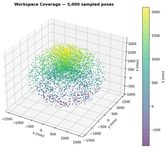
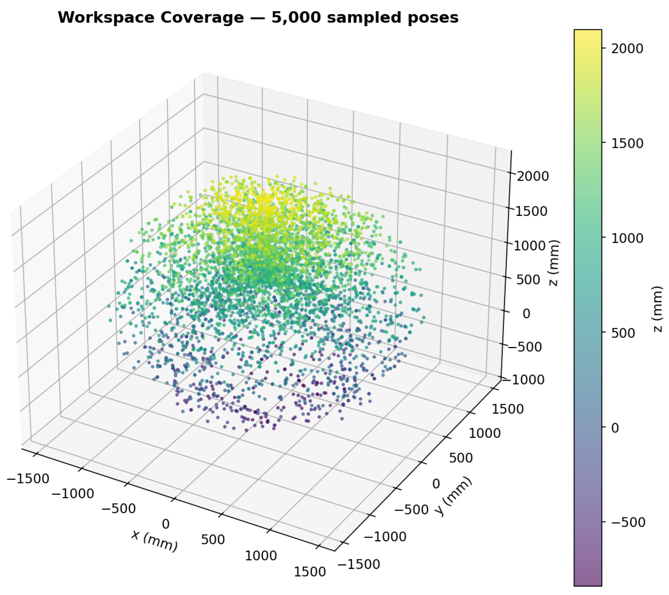
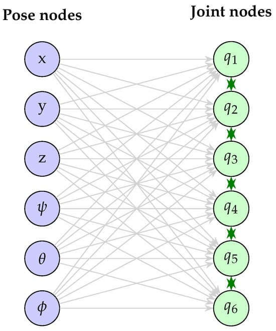
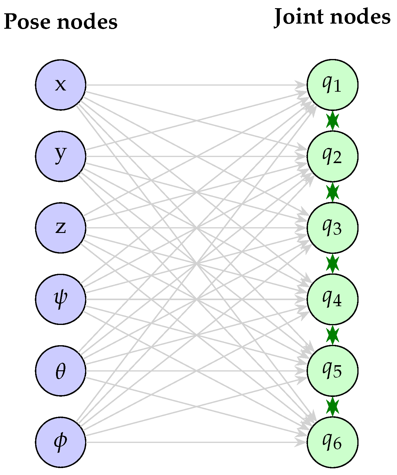
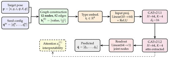
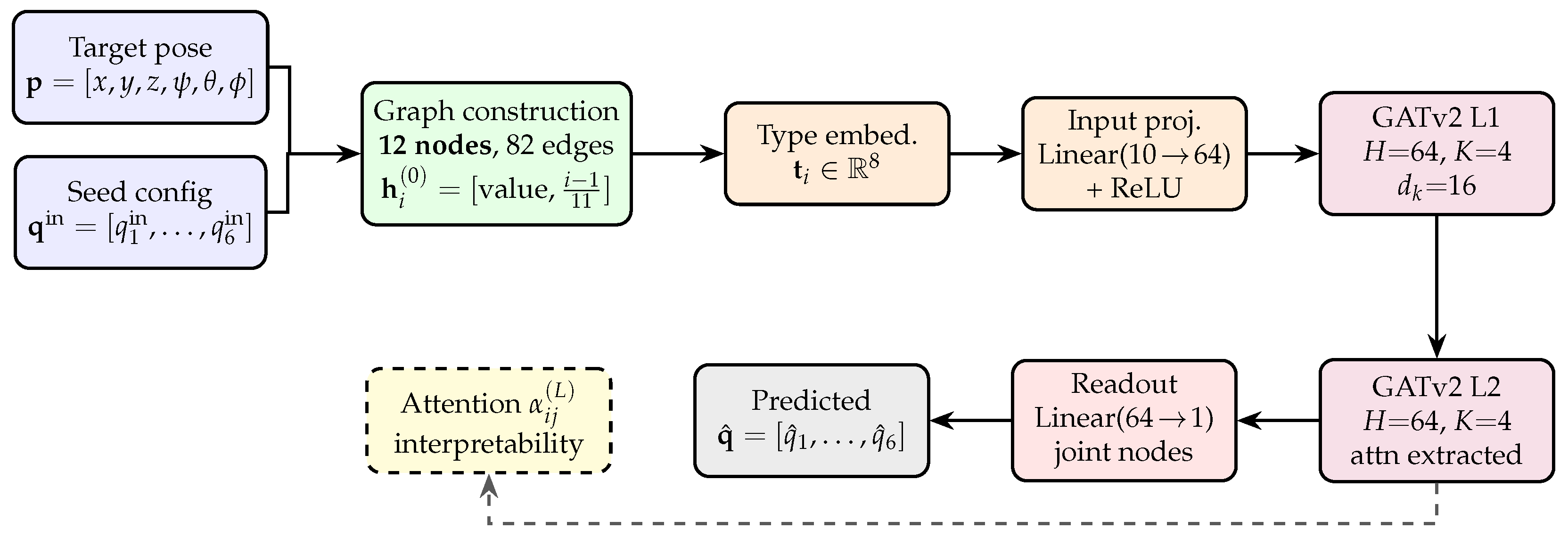
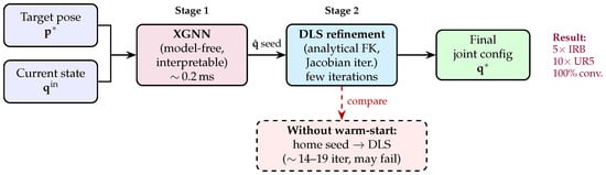
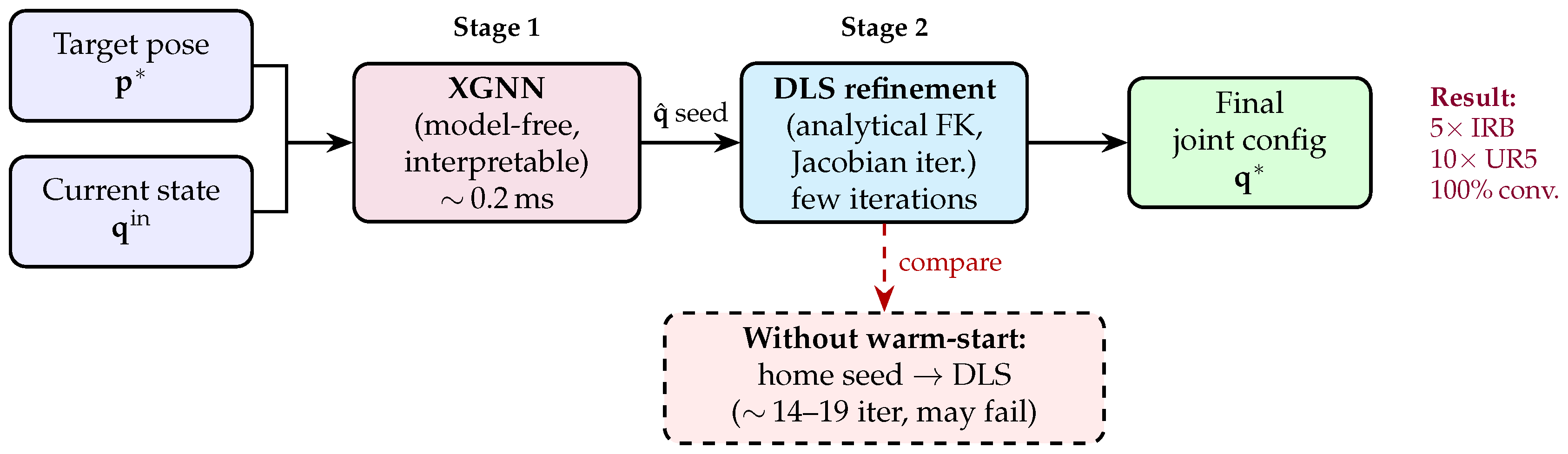
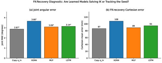
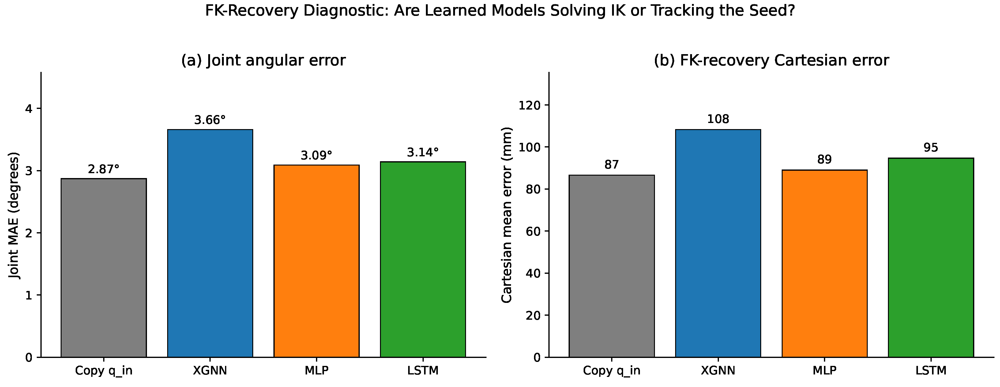
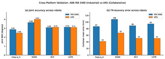
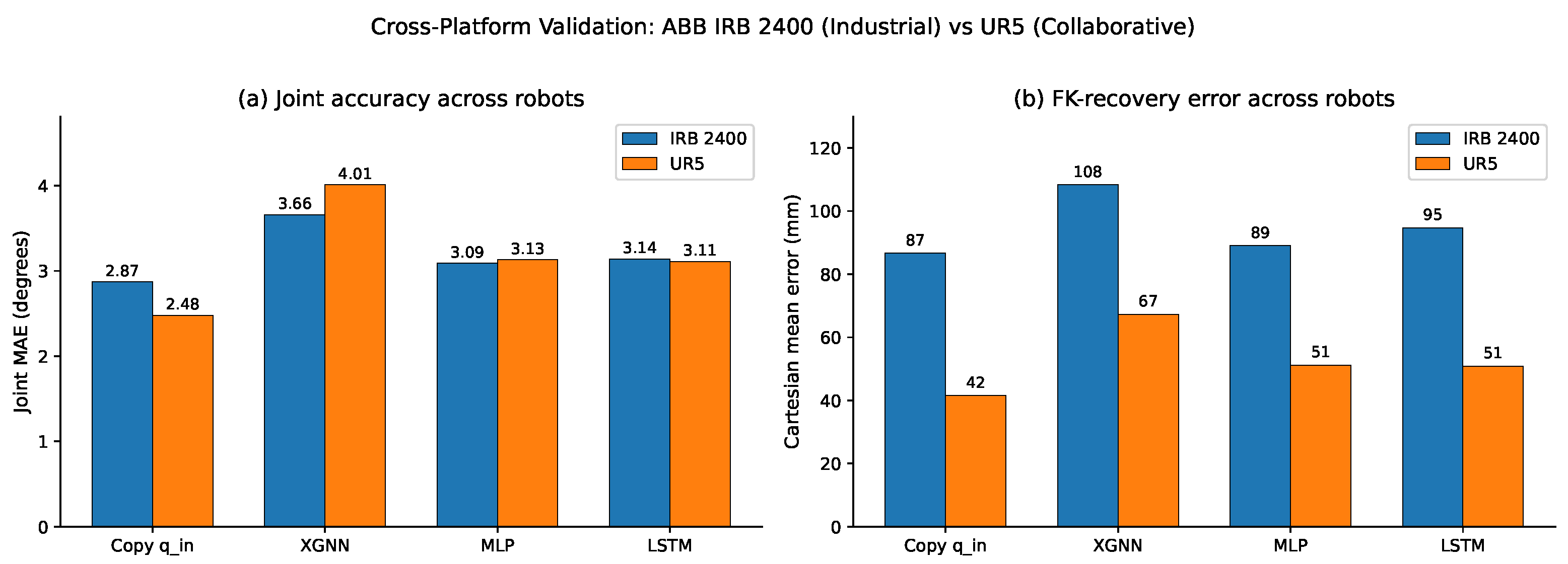
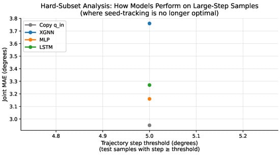
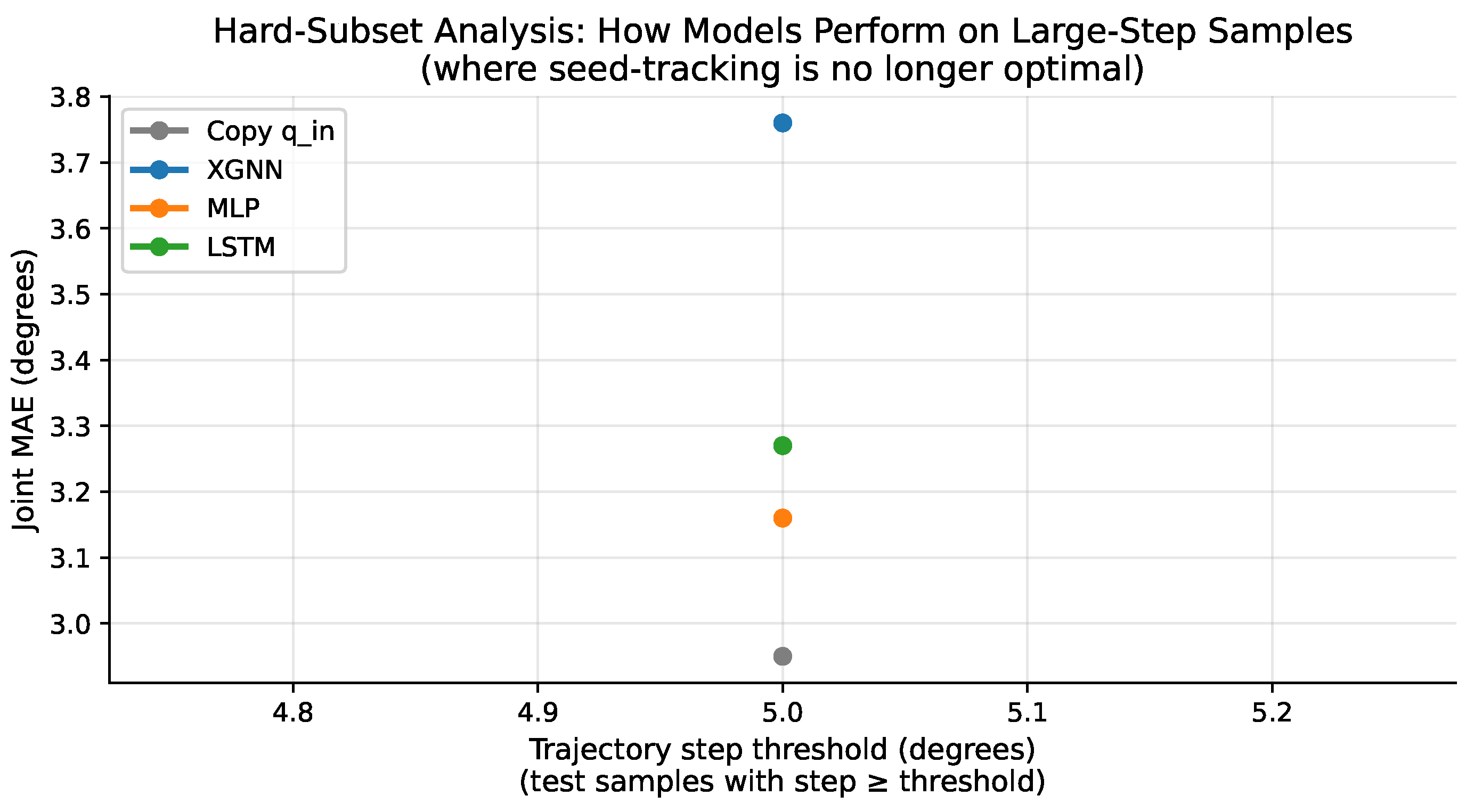
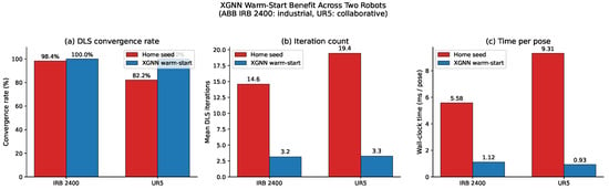
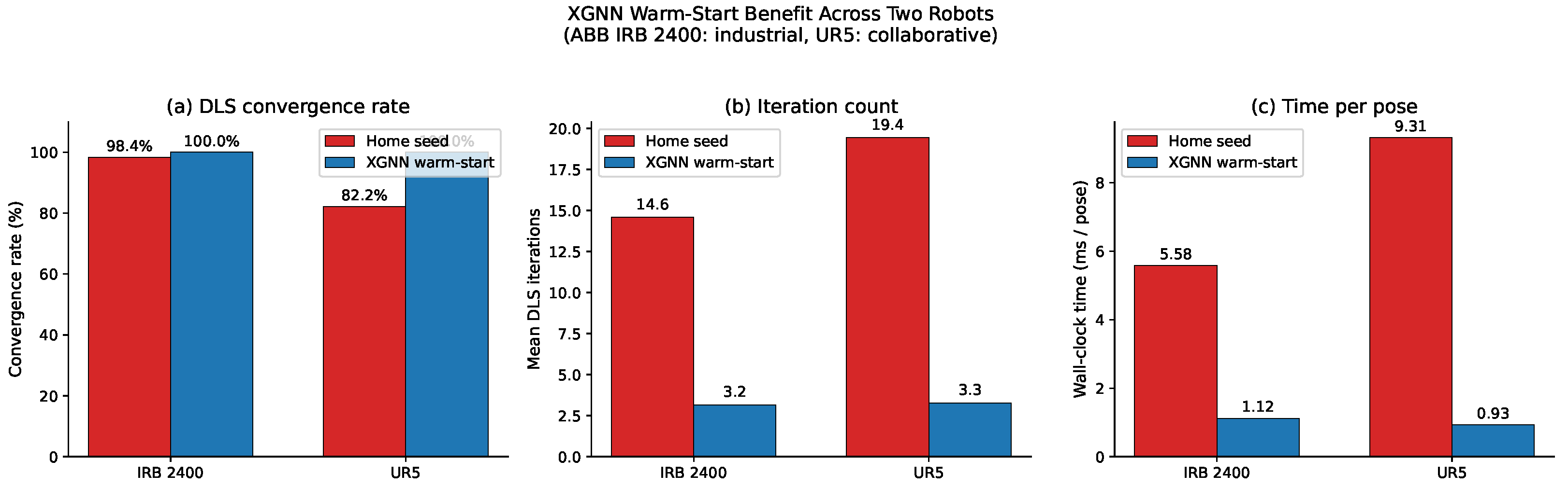
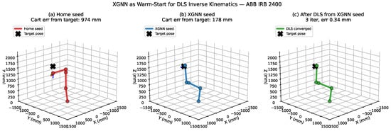
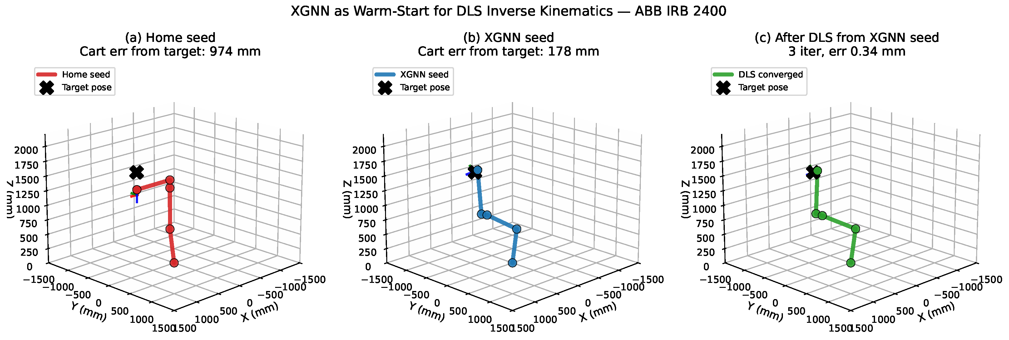
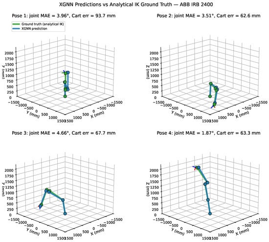
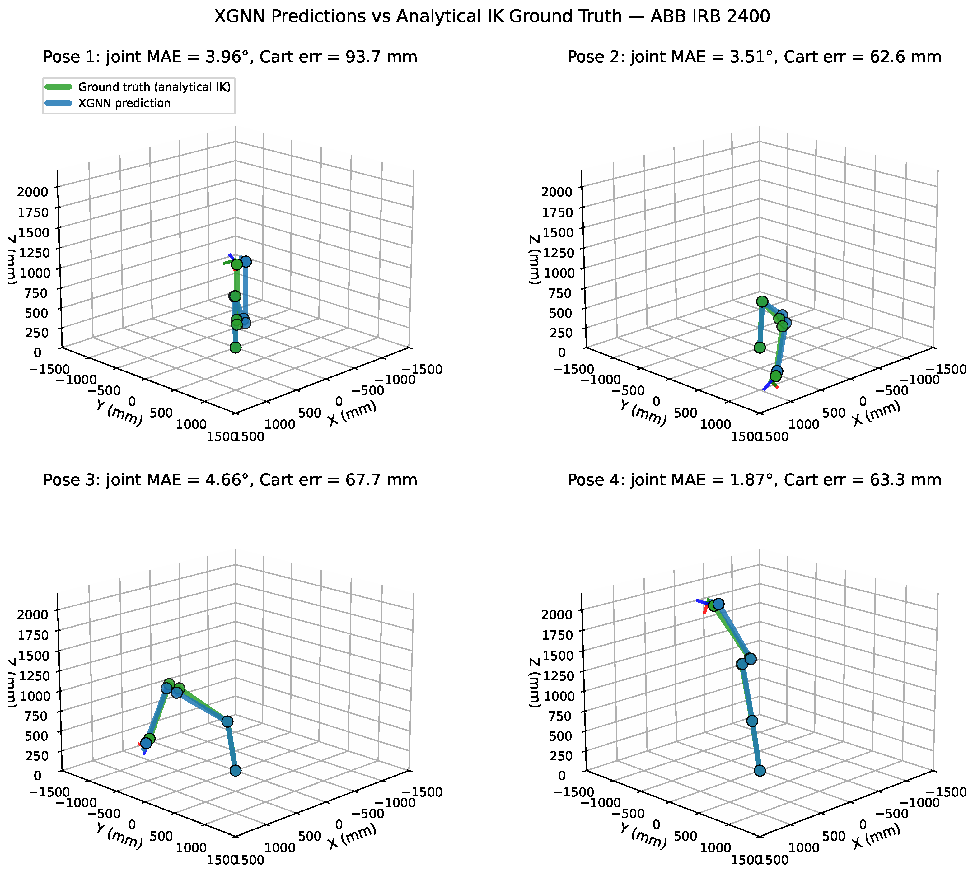
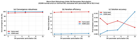
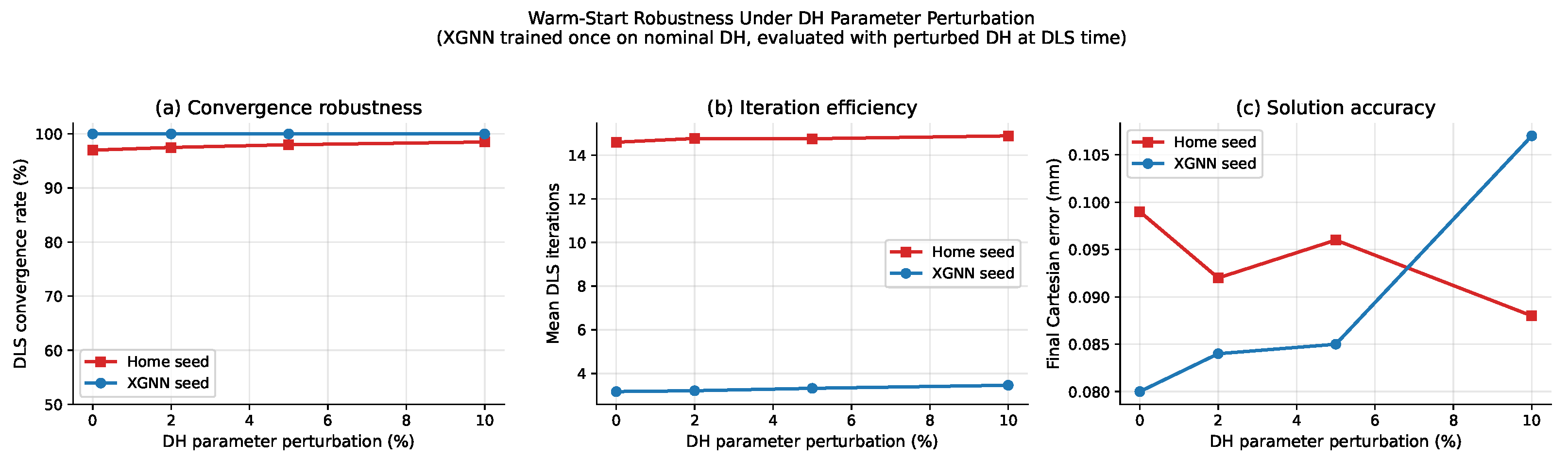
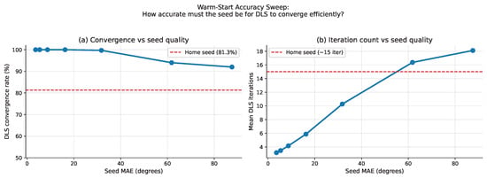
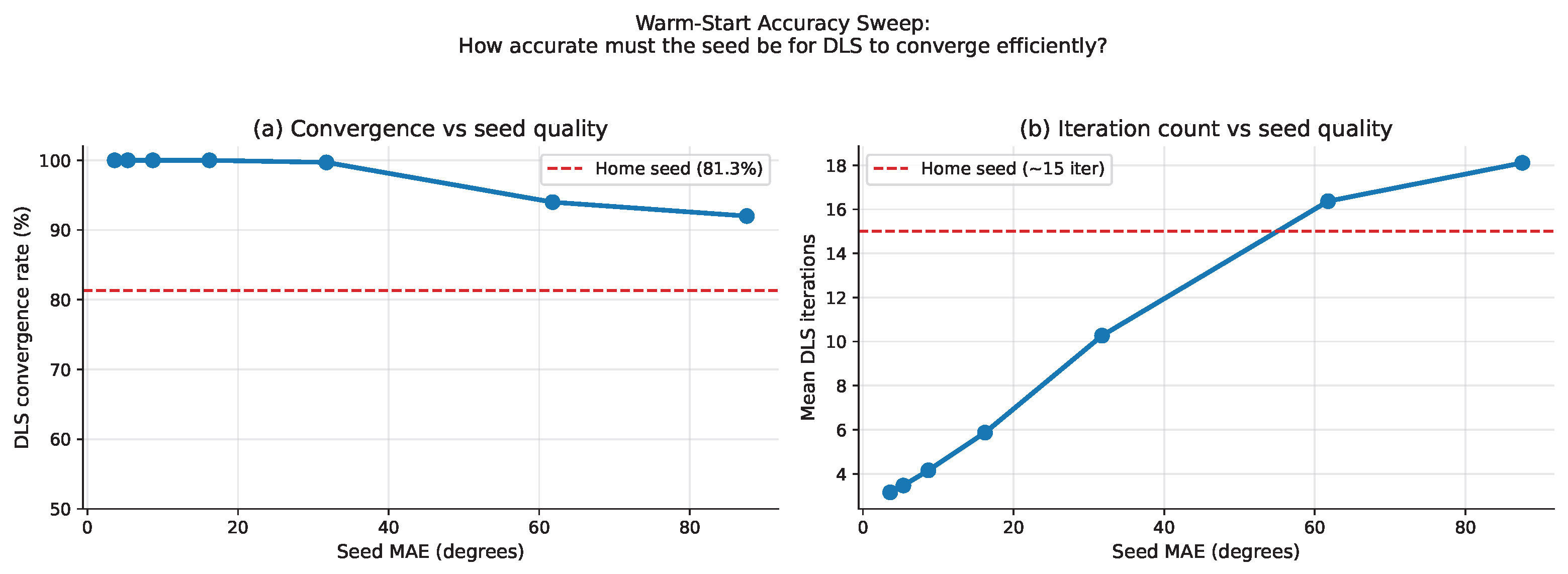
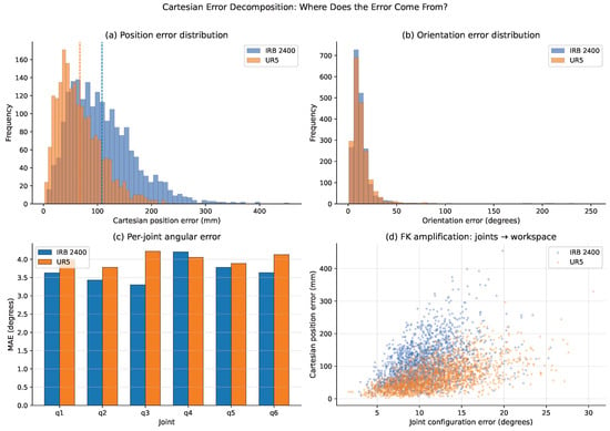
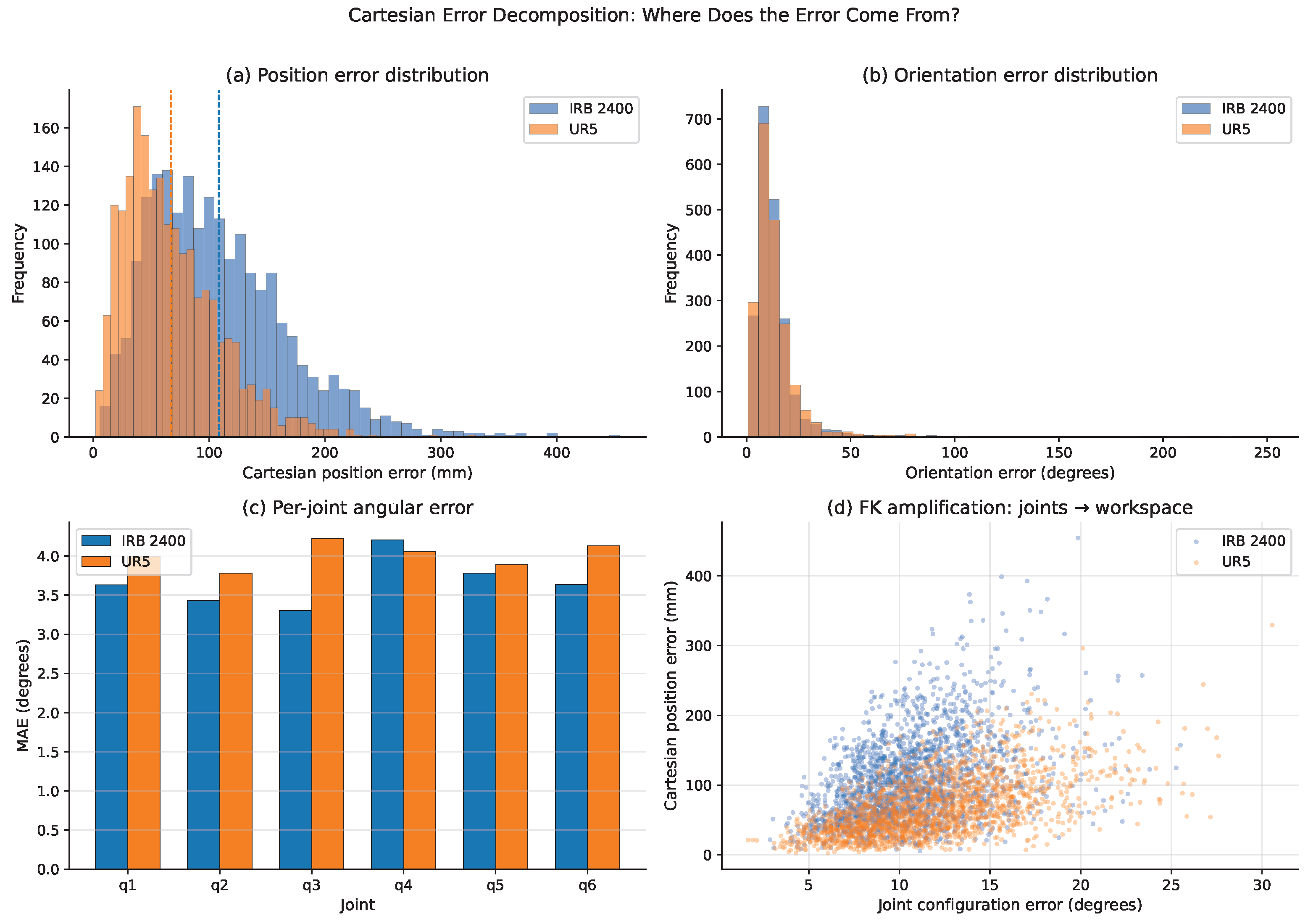
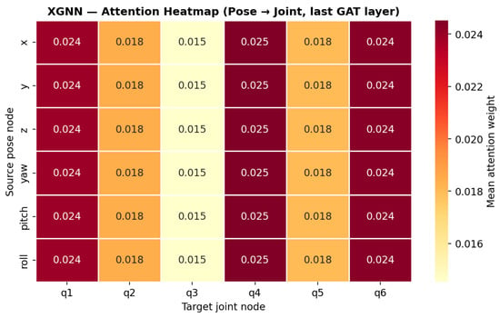
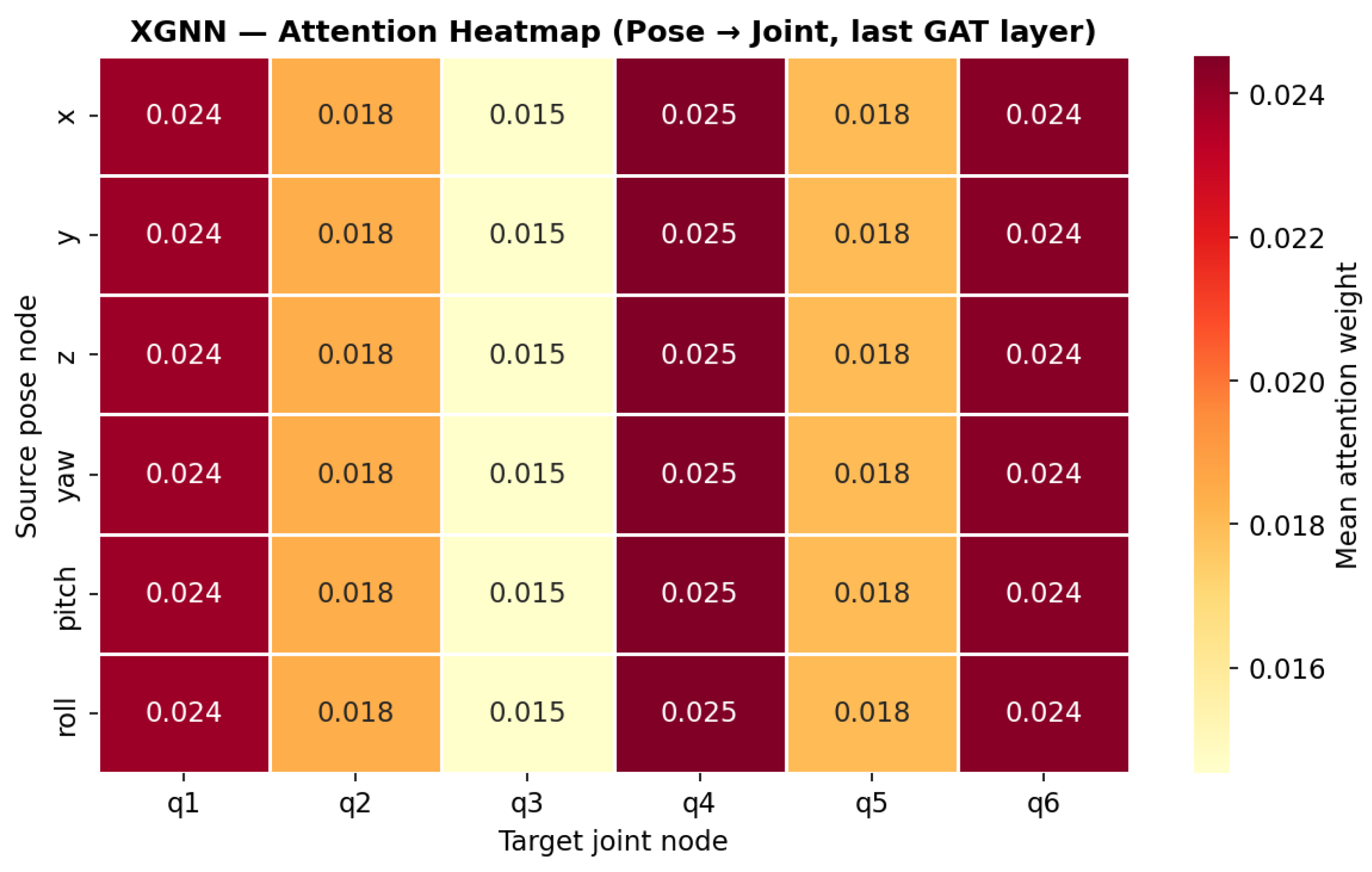

Disclaimer/Publisher’s Note: The statements, opinions and data contained in all publications are solely those of the individual author(s) and contributor(s) and not of MDPI and/or the editor(s). MDPI and/or the editor(s) disclaim responsibility for any injury to people or property resulting from any ideas, methods, instructions or products referred to in the content. |
© 2026 by the authors. Licensee MDPI, Basel, Switzerland. This article is an open access article distributed under the terms and conditions of the Creative Commons Attribution (CC BY) license.