


Abstract
Receiver mobility complicates channel state information (CSI) acquisition in fluid antenna system (FAS)-assisted grant-free random access (GFRA), because user activity and multi-port channels evolve across pilot frames. Existing FAS acquisition methods are mainly frame-wise, while temporal recovery schemes do not directly combine receiver geometry with Doppler information. This article proposes geo-temporal expectation-maximization approximate message passing (GT-EM-AMP), which transfers posterior information between frames and refines the channel prior using receiver trajectory, effective Doppler, and coarse geometry. The proposed recursion preserves the low-complexity structure of EM-AMP while introducing only limited additional state updates. Simulations over an SNR range from to 8 dB show that GT-EM-AMP achieves lower channel-estimation error and a favorable activity-detection tradeoff relative to static, temporal-only, geometry-only, and greedy baselines. Ablation, robustness, mobility, scalability, and statistical evaluations characterize the operating range of GT-EM-AMP and show that its activity-detection advantage depends on the SNR regime. GT-EM-AMP introduces modest runtime and memory overhead relative to static EM-AMP. The evaluation focuses on short acquisition windows with coarse geometry information under a Jakes-type temporal model.
1. Introduction
Grant-free random access (GFRA) supports sporadic massive connectivity by allowing active users to transmit without grant scheduling, thereby reducing signaling overhead and access latency in Internet-of-Things (IoT) and other intermittent uplink services [1,2]. Recent studies have further connected unsourced random access with slow fluid-antenna multiple access and FAS-assisted integrated sensing and communications, and have examined finite-blocklength FAS performance under spatial block-correlation channel models [3,4,5]. In this setting, the receiver must jointly detect active users and estimate their channels from a shared pilot observation. This task is naturally formulated as a structured sparse-recovery problem [6]. Approximate message passing (AMP) and expectation-maximization AMP (EM-AMP) provide an attractive accuracy–complexity tradeoff for such large-scale inference tasks [7,8]. Fluid antenna systems (FASs) further introduce a reconfigurable port domain, allowing the receiver to observe geometry-dependent channel variations across candidate ports [9,10,11]. Geometry- and mobility-aware channel modeling has also been investigated for FAS-UAV links, movable-antenna UAV-to-UAV channels, RIS-enabled air-ground channels, and near-field large-scale MIMO systems [12,13,14,15]. This port-domain diversity is attractive for CSI acquisition, but it also makes the channel statistics more sensitive to receiver geometry and motion.
Recent FAS CSI acquisition studies have mainly followed model-driven designs, including sparse Bayesian reconstruction, low-complexity EM-AMP schemes exploiting geographical diversity, and geographical/angular-information-aided activity detection and channel estimation [16,17,18]. Recent analyses have also characterized activity-detection limits in conventional and fluid antenna systems and explored learned AMP-type reconstruction under Karhunen–Loeve modeling for FAS channels [19,20]. Related work on fluid antenna multiple access and spatial channel modeling further shows that port reconfigurability can reshape the channel statistics available to the receiver [10,11]. These studies establish the usefulness of FAS structure for CSI acquisition. However, most of them assume a static receiver or treat each frame as an independent estimation problem. The geo-prior EM-AMP method in [17], for example, uses geographical diversity for static FAS CSI acquisition but does not model receiver-motion-induced channel evolution.
Beyond the FAS literature, dynamic sparse recovery has been studied through temporal AMP, dynamic sparse Bayesian learning, Bayesian tracking, and learned AMP-type reconstruction [20,21,22,23]. These methods show that temporal support evolution, state-space tracking, and trainable iterations can improve sparse inference for time-varying signals. However, they are not directly tailored to mobile FAS-GFRA, where the receiver observes a row-sparse multi-port pilot matrix and where the prior statistics depend jointly on receiver geometry, port-domain fading, and Doppler-induced temporal correlation. Tracking-based methods generally rely on explicit state-space models for the channel coefficients, whereas learned AMP variants require representative training data and offer a different tradeoff between data adaptivity and model transparency. The remaining gap lies in a model-driven mechanism that translates mobile FAS geometry and Doppler-induced temporal correlation into the prior parameters used by low-complexity EM-AMP inference. This article addresses this gap by designing a recursive prior-learning scheme that is physically interpretable, compatible with the row-sparse GFRA observation model, and computationally comparable to frame-wise EM-AMP.
CSI acquisition for a mobile-receiver FAS remains challenging for three reasons. First, the GFRA observation must preserve the row-sparse structure induced by sporadic user activity, because this structure supports joint activity detection and channel estimation. Second, the channel prior should evolve with the receiver trajectory rather than be reinitialized independently in each frame, which requires a principled way to incorporate mobility-induced temporal correlation. Third, receiver motion changes the large-scale geometry and Doppler characteristics, making the prior statistics frame dependent and difficult to estimate reliably at low signal-to-noise ratios (SNRs). The resulting challenge is to combine row-sparse support inference, mobility-aware cross-frame prediction, and geometry-based prior stabilization while retaining the low-complexity scalar updates of EM-AMP.
To meet this challenge, this article develops a geo-temporal EM-AMP framework for CSI acquisition in FAS-assisted GFRA with a mobile receiver. The key idea is to map mobile-receiver physical side information, including receiver trajectory, effective Doppler, and geometry-dependent fading, into recursive Bernoulli–Gaussian prior parameters for EM-AMP denoising. In this way, the proposed method links mobility-induced channel evolution with low-complexity sparse Bayesian inference while preserving the scalar-update structure of conventional EM-AMP. The resulting framework extends frame-wise FAS CSI acquisition toward mobility-aware recursive estimation.
GT-EM-AMP extends frame-wise static EM-AMP by propagating posterior information across frames, and differs from fixed-correlation temporal EM-AMP by deriving user-specific temporal correlation from mobility-induced effective Doppler. It further combines recursive temporal prediction with geometry-based variance anchoring, which is absent from geo-prior EM-AMP, and performs probabilistic support-and-channel inference rather than the temporally smoothed greedy recovery used by SS-SOMP+LS. In contrast to general dynamic sparse-recovery and learned AMP methods, the proposed prior update is tailored to the row-sparse multi-port FAS-GFRA observation model. The principal contribution is therefore a physically interpretable geo-temporal prior recursion integrated into the EM-AMP framework.
The main contributions are summarized as follows:
- Mobile FAS-GFRA support-and-channel inference model: A mobile-receiver FAS-assisted GFRA CSI acquisition problem is formulated as a row-sparse multi-port inference task, where sporadic user activity, port-domain channel coefficients, and receiver-motion-induced temporal variation are jointly considered.
- Doppler-aware recursive prior learning: A geo-temporal EM-AMP framework is developed to incorporate receiver trajectory and effective Doppler into recursive Bernoulli–Gaussian prior prediction. This provides a physically interpretable way to propagate prior information across frames instead of reinitializing the CSI estimator independently in each frame.
- Geometry-stabilized variance regularization: A geometry-aware variance regularization mechanism is introduced to stabilize EM learning under weak pilot observations. The mechanism uses large-scale geometry information as a soft variance anchor while retaining the EM-updated posterior statistics as the dominant source of adaptation.
- Comprehensive operating-range evaluation: Extensive simulations assess component contributions, parameter sensitivity, model mismatch, activity screening, scalability, mobility robustness, statistical significance, and computational cost. The results characterize both the performance gains and the operating range of GT-EM-AMP under the considered short-horizon setting.
2. Materials and Methods
2.1. System Model
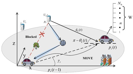
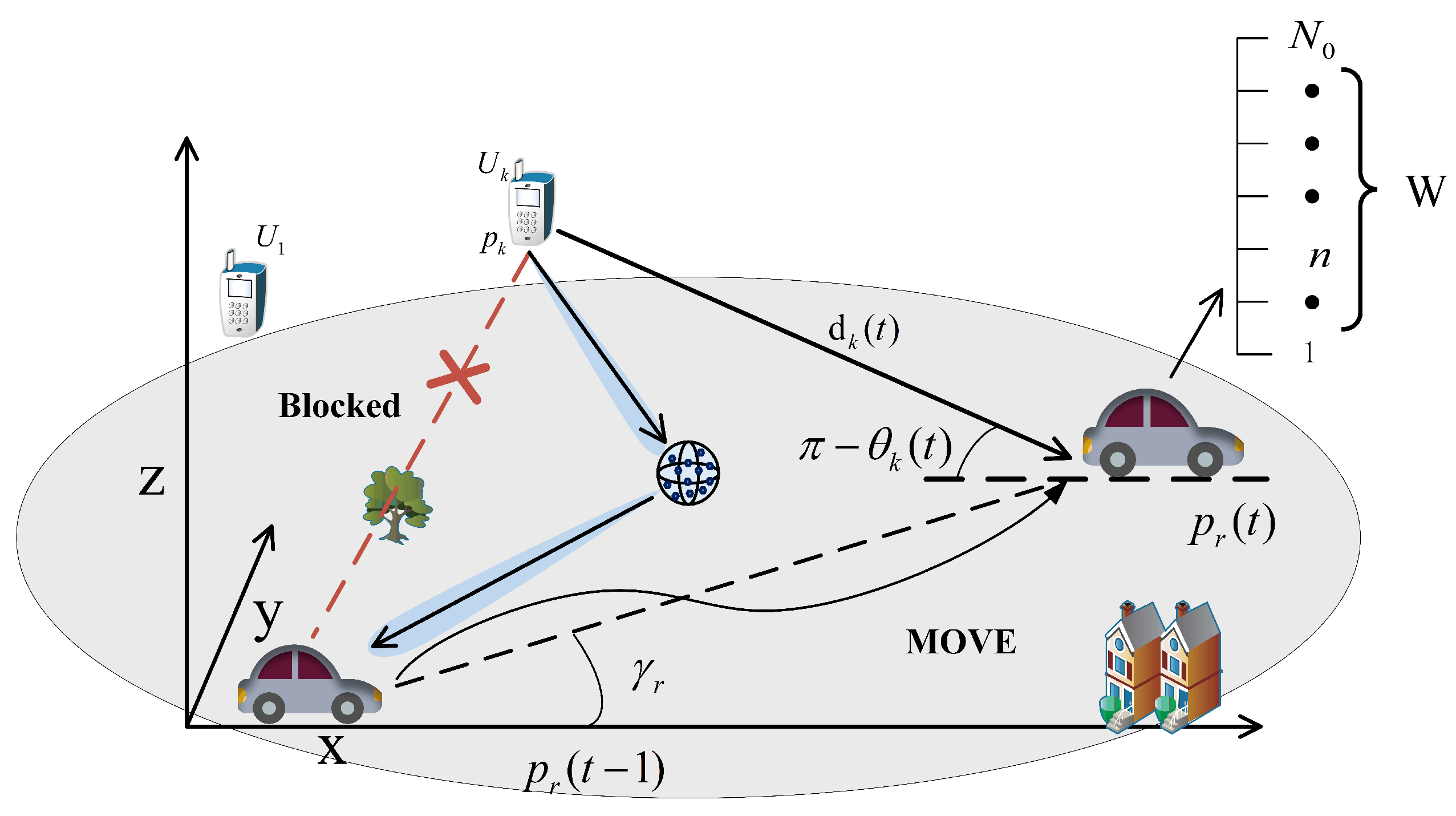
As illustrated in Figure 1, we consider an uplink GFRA scenario in which K potential single-antenna users communicate with a mobile vehicular receiver equipped with an FAS having candidate ports. During CSI acquisition, the receiver observes the multi-port pilot response over the candidate FAS ports rather than selecting a single port for training. Receiver motion makes the user-to-receiver distance, angle of arrival (AoA), and Doppler characteristics frame dependent, thereby inducing explicit temporal structure in the port-domain channel.
Figure 1.
Illustration of the considered uplink grant-free random access (GFRA) system with a mobile vehicular receiver equipped with a fluid antenna system (FAS). The black dots in the aperture inset denote the observed candidate FAS ports.
Let denote the frame index, and let the corresponding physical time be , where is the frame duration. At frame t, the received pilot matrix is modeled as
where denotes the received signal matrix, is the known normalized random pilot matrix of length G, is the unknown row-sparse channel matrix, and is additive white Gaussian noise whose entries follow . The kth row of is written as , where is the activity indicator of user k and is the corresponding port-domain channel. Since only a small subset of users is active in each frame, has a row-sparse structure. This row sparsity is induced by user activity rather than by port selection. An active user contributes a channel vector across all observed candidate ports, whereas an inactive user contributes an all-zero row. This is consistent with multi-port pilot acquisition during training. Final data transmission may subsequently select one or several ports according to the receiver-side FAS policy. The Bernoulli part of the prior represents this user-level support, while the Gaussian part provides a tractable statistical approximation for the aggregate small-scale coefficient. Thus, the Bernoulli–Gaussian model serves as an aggregate inference prior for the port-domain coefficient after multipath superposition, rather than as a path-level distributional assumption. The pilot matrix is generated independently of user activity and normalized column-wise, which provides a common pilot-energy basis for all compared algorithms. The CSI acquisition task is therefore a joint support-and-coefficient inference problem: the receiver must identify the active rows of and estimate the corresponding multi-port channel coefficients from the noisy shared pilot observation. Over the short GFRA estimation window considered here, the receiver follows approximately constant-speed linear motion in the horizontal plane, and the receive FAS array center is initially located at
where is the fixed receive installation height. The platform moves with constant speed and horizontal heading angle , measured counterclockwise from the positive x-axis, so that its velocity vector is
Accordingly, the receiver position at frame t becomes
Let the location of user k be
Then, the user-to-receiver distance at frame t is
and the dominant AoA in the azimuth plane is given by
The corresponding large-scale fading coefficient (LSFC) is modeled as
where is a reference path-loss constant and is the path-loss exponent.
Consider a linear FAS aperture of length W with uniformly distributed candidate ports. The location of the nth port along the aperture is , . For an incident wave with AoA , the normalized steering response is
where denotes the carrier wavelength. The symbol is used here to avoid confusion with the activity probability in the subsequent EM-AMP recursion. Assume that the channel of user k consists of effective propagation paths. The resulting port-domain channel is modeled as
where , , and denote the gain, phase, and AoA of the lth path, respectively.
The adopted operating assumptions include fixed or slowly varying access-device positions over the short estimation horizon, a Jakes-type temporal correlation law, and geometry-aided variance anchoring. These assumptions define the intended operating regime and govern the recursive prior update, while the linear AMP observation model remains unchanged. Over the short pilot horizon considered here, receiver motion is treated as the dominant source of temporal channel variation. The Jakes-type law provides a compact Doppler-to-correlation mapping under local scattering, while the geometry terms may be obtained from positioning, map-aided localization, or coarse long-term channel measurements. The proposed variance anchoring uses such coarse distance and angle information as soft prior side information rather than exact channel knowledge. Robustness to imperfect side information is evaluated through the geometry/Doppler mismatch experiment in the simulation section.
Receiver mobility induces a Doppler shift on each propagation path. Let denote the propagation-direction unit vector of the lth path. The radial relative velocity is defined as
where is the velocity of user k. For the short-horizon access setting considered here, access-device motion is neglected—i.e., —so receiver motion dominates the temporal variation. This stationary-device assumption is adopted in the default experiments. This assumption is relaxed in the moving-user robustness study by assigning nonzero user velocities and recomputing the relative Doppler according to (11)–(14). In the adopted azimuthal description, the horizontal projection of is parameterized by , so the projected receiver displacement determines the phase rotation below. The path-wise Doppler shift is then given by
and the corresponding phase evolves as
The AMP denoiser operates on the aggregated coefficient rather than on individual physical paths. Therefore, the multipath Doppler set is represented by the power-weighted effective Doppler
This quantity serves as a tractable scalar surrogate for the multipath Doppler set in the recursive prior model. To connect the physical channel evolution to the denoiser prior, the aggregated coefficient is modeled by the first-order Gauss–Markov recursion
where is a zero-mean circularly symmetric complex Gaussian innovation term with variance . Under the commonly adopted local-scattering/wide-sense stationary uncorrelated scattering (WSSUS)-type approximation, the temporal correlation coefficient is modeled by the Jakes-type expression , where is the zeroth-order Bessel function. This gives a compact mobility-aware correlation model for recursive inference. To exploit both user sparsity and temporal correlation, each coefficient is assigned a dynamic Bernoulli–Gaussian prior
where , , and denote the activity probability, shared nonzero mean, and nonzero variance, respectively. Conditioned on the posterior statistics of frame , the predicted prior parameters at frame t are
Equations (14)–(19) form the geo-temporal prior-update chain used by GT-EM-AMP: receiver trajectory determines the effective Doppler, the effective Doppler determines the Jakes-type correlation coefficient, and this coefficient predicts the mean and variance of the Bernoulli–Gaussian denoising prior for the next frame. This prior-update chain converts receiver-side physical information into the statistical quantities required by the recursive support-and-channel inference problem. The activity-probability recursion in (17) is used as a short-horizon prior propagation rule for burst-level GFRA, where the activity information learned from the previous pilot frame remains informative for the next frame.
Accordingly, the predicted Bernoulli–Gaussian prior at frame t becomes
Table 1 summarizes the main notation used in the system model and GT-EM-AMP algorithm.
Table 1.
Main notation used in the system model and GT-EM-AMP algorithm.
2.2. Problem Formulation and Proposed GT-EM-AMP Scheme
Given the observation sequence , the pilot matrix , and the dynamic Bernoulli–Gaussian prior in (20), the receiver aims to infer, for each frame t, both the active-user support and the corresponding row-sparse multi-port channel matrix. Equivalently, the inference objective is to obtain the posterior activity probabilities and channel posterior statistics under the recursively predicted prior. This problem couples discrete user activity, continuous port-domain channel coefficients, and cross-frame prior evolution. Exact Bayesian inference is therefore computationally prohibitive when the numbers of candidate users, pilot dimensions, and FAS ports are large. GT-EM-AMP addresses this difficulty by preserving the scalar-update structure of EM-AMP while exploiting mobility-induced temporal correlation. For each frame, the prior is predicted from the previous-frame posterior, refined by AMP using the current observation, and updated by EM with geometry-aware variance stabilization. Algorithm 1 summarizes the recursive structure of GT-EM-AMP, where t and denote the frame and AMP-iteration indices, respectively. The geometry- and Doppler-dependent quantities used by the recursive prior are defined in (11)–(20), while the geometry-aware variance update is given in (40)–(42). The corresponding default implementation parameters are specified in the numerical-evaluation setup. In Algorithm 1, denotes the innovation-variance sequence obtained from and the geometry-derived reference according to .
The numerical damping factor is used only to improve the numerical stability of the iterative AMP recursion and does not modify the Bernoulli–Gaussian prior model. Its default value is specified with the numerical simulation parameters.
| Algorithm 1: GT-EM-AMP for Mobile-Receiver FAS CSI Acquisition |
|
The recursive prior states are initialized as follows. Specifically, is initialized by the nominal activity ratio , is set to zero, and is initialized from the geometry-aided large-scale fading level after calibration by . The innovation variance is modeled as , where controls the process uncertainty rather than the observation-noise power. Larger values permit faster frame-to-frame prior variation and weaken temporal persistence. The values and are used as conservative fixed settings rather than being retuned for individual SNRs or mobility conditions. The former keeps the EM-updated variance as the dominant component while retaining a nonzero geometry-based correction, whereas the latter limits excessive diffusion of the propagated prior over adjacent frames. Both values are held fixed throughout the reported SNR, mobility, port-number, active-load, and pilot-length experiments. The sensitivity results reported in the numerical evaluation show that the reported performance remains stable over the tested parameter ranges. The inner AMP loop stops when the relative posterior-mean change
falls below or when iterations are reached. After the inner AMP recursion terminates, active users are selected using the row score
When the active-user cardinality is available, the receiver selects the users with the largest row scores. When the cardinality is unavailable, threshold-based activity screening can be applied to the estimated activity probabilities. For the controlled known-cardinality comparisons, all AMP-based methods use the same cardinality-based support selection rule. The inner AMP recursion used to produce these posterior quantities is detailed next. For a fixed frame t, let denote the AMP iteration index. Denote by and the current posterior mean and variance estimates, respectively. The variance of the linear mixture at output node is
and the corresponding mean is
The second term in (24) is the full Onsager subtraction term required by AMP. It compensates for the correlation buildup caused by iterative message reuse and preserves the approximate scalar-Gaussian decoupling that underlies AMP.
Under the additive white Gaussian noise (AWGN) output channel, the posterior mean and variance of the linear mixture variable are
The resulting residual messages are updated as
Given the output-node messages, the pseudo-observation variance and mean at input node are
These quantities define the equivalent scalar Gaussian channel with . This scalar channel enables decoupled denoising at each input node.
Combining this scalar channel with the predicted Bernoulli–Gaussian prior in (20) yields the posterior distribution in (31), while the corresponding coefficient-level posterior support probability is given by (32):
Here, denotes the coefficient-level posterior support probability of . The variance and mean of the Gaussian component are
and the posterior mean and variance are updated as
Thus, the denoiser uses both the instantaneous pseudo-observation and the mobility-aware prior predicted from the previous frame. This joint use of current observations and cross-frame prior prediction distinguishes GT-EM-AMP from frame-wise static EM-AMP.
After the inner AMP recursion terminates at frame t, the posterior statistics produced by the Bernoulli–Gaussian denoiser are used to update the hyperparameters in closed form. The activity probability is estimated by averaging the posterior support probabilities across all candidate ports:
Since a shared nonzero mean is adopted across ports, the mean parameter is updated as
The EM-updated shared mean is then propagated as the prior mean state for the next-frame recursion, i.e., . The corresponding EM-updated nonzero variance is
To stabilize the propagated variance, a geometry-aware reference is introduced as
and fused with the EM-updated variance as
followed by clipping
Here, rescales the geometry-derived large-scale fading to the variance level used in EM inference. The parameter controls the fusion strength between the EM-updated and geometry-anchored variances. This geometry-aware anchoring suppresses unstable variance drift under weak observations. Values of close to one place greater weight on the EM-updated variance, whereas smaller values strengthen the geometry-derived correction. In the simulations, is calibrated once at initialization by the median-ratio rule described in Section 3 and is then held fixed within each trial.
The dominant computational cost remains the AMP linear-mixing updates in (23) and (24) and (29) and (30), whose per-iteration complexity is . By contrast, cross-frame prior prediction and geometry-aware refinement require only and operations, respectively. The additional steps are limited to scalar prior prediction, geometry-aware variance refinement, and storage of user- and port-level prior parameters. Hence, the geo-temporal refinement preserves the dominant linear-mixing complexity while introducing limited additional arithmetic and persistent-state storage. Including the reused pilot matrix, the output-node statistics, and the user-port posterior statistics, the working memory scales as . Only the previous-frame user-port posterior statistics and user-level prior parameters must be retained across frames, giving a persistent cross-frame state of .
3. Results
Table 2 summarizes the simulation settings used in the numerical evaluation. Unless otherwise stated, each Monte Carlo trial uses the same user geometry and pilot realization for all compared algorithms.
Table 2.
Simulation parameters used in the numerical evaluation.
Unless otherwise stated, and are fixed at their default values for all reported operating points and are not retuned separately for different SNRs, receiver speeds, pilot lengths, user loads, or FAS port numbers.
The AMP-based methods use the same pilot matrix, Monte Carlo seeds, maximum iteration count, stopping tolerance, and known-cardinality support selection rule in the main comparisons. For each Monte Carlo trial, is generated with i.i.d. entries and then normalized column-wise to unit norm; the same is used across all frames in that trial. For the controlled simulations, is computed once at the beginning of each Monte Carlo trial using a median-ratio scale alignment between the simulation-generated active-row channel power and the corresponding nominal geometry variance. The resulting scalar is fixed throughout the trial, and the same calibration procedure is used for GT-EM-AMP and geo-prior EM-AMP. Together with the initialization rules in Section 2.2, these settings define the numerical configuration used in all experiments unless otherwise stated. The default values of and listed in Table 2 are used for geometry-aware variance fusion and prior innovation scaling, respectively. The damping factor listed in Table 2 is used only as a numerical-stability implementation detail for the geometry-fused AMP variants. Unless otherwise stated, the main SNR comparisons report the median over 80 matched Monte Carlo trials, with interquartile range (IQR) error bars. The numbers of trials and uncertainty measures used in the ablation, robustness, scalability, mobility, runtime, and statistical studies are specified in the corresponding figure and table captions. The threshold-based activity screening reported in Table 3 uses 40 Monte Carlo trials. All simulations were run in MATLAB R2024b (The MathWorks, Inc., Natick, MA, USA) with random seed 20260407 on a Windows 11 (Microsoft Corporation, Redmond, WA, USA) workstation equipped with an AMD Ryzen 9 7945HX CPU (Advanced Micro Devices, Inc., Santa Clara, CA, USA), 32 logical processors, and 32 GB RAM. No GPU acceleration was used.
Table 3.
Threshold-based activity screening under unknown- using .
The evaluation compares GT-EM-AMP with four representative model-driven baselines. Frame-wise static EM-AMP removes both temporal recursion and geometry/Doppler information. Temporal EM-AMP uses a global fixed correlation coefficient , shared by all users and frames, but does not use user-specific Doppler or geometry-aware variance anchoring. Geo-prior EM-AMP keeps the geometry-based prior in each frame but removes temporal recursion. Score-smoothed SOMP+LS (SS-SOMP+LS) is included as a lightweight tracking-inspired greedy comparator. It combines simultaneous orthogonal matching pursuit with first-order temporal score smoothing and least-squares coefficient estimation [24]. This baseline serves as a lightweight non-AMP comparator under the same pilot and channel settings.
The score-smoothed SOMP+LS baseline is implemented by the following tracking-inspired score update:
The largest smoothed scores form the detected support. On this support, the coefficient estimate is obtained by least squares and then smoothed as
The metrics are chosen to match the two components of the formulated inference problem. ADE evaluates active-support recovery, whereas support-matched and all-active NMSE evaluate multi-port channel estimation under different support assumptions. The activity-detection error is defined as , where and denote the true and detected active-user sets, respectively. The support-matched normalized mean square error (NMSE) is computed only over correctly detected active users:
We also report an all-active NMSE over the true active rows:
This metric penalizes both missed active users and channel-coefficient errors, and is therefore stricter than support-matched NMSE.
In the controlled known- simulations, the largest row scores are retained to compare algorithms under the same support-cardinality constraint. In the unknown- screening test, the estimated activity probabilities are thresholded to form a cardinality-free activity decision, as examined in Table 3. The detected set is formed by without enforcing a fixed cardinality. A fixed threshold is used across all tested SNR values. At very low SNR, this fixed threshold favors precision over recall; at and 0 dB, it achieves high precision and recall, leading to substantially improved F1 scores without retuning.
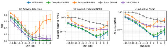
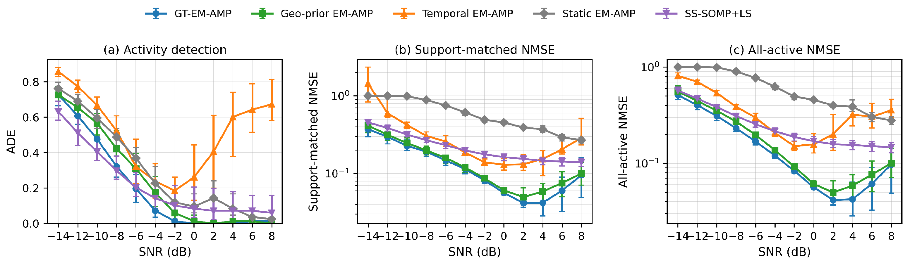
Figure 2 evaluates the SNR range from to 8 dB. GT-EM-AMP reduced both support-matched and all-active NMSE relative to static EM-AMP, temporal EM-AMP, and SS-SOMP+LS across the tested range. Relative to the static and temporal EM-AMP baselines, GT-EM-AMP also reduced ADE from dB upward. SS-SOMP+LS remained competitive for activity detection at the lowest SNR values, but exhibited higher channel-estimation error. At dB, the median support-matched NMSE of GT-EM-AMP was 0.227, compared with 0.422 for temporal EM-AMP, 0.990 for static EM-AMP, and 0.317 for SS-SOMP+LS. The corresponding all-active NMSE values were 0.311, 0.538, 0.992, and 0.384, respectively. At the high-SNR endpoint, the geo-prior baseline approached GT-EM-AMP because current-frame observations became more reliable. The slight NMSE fluctuation remained within the IQR band and did not alter the performance ordering relative to the static and temporal baselines. This behavior indicates that the recursive geo-temporal prior is most useful when current-frame pilots alone cannot reliably stabilize both support detection and coefficient estimation.
Figure 2.
Wide-SNR comparison of GT-EM-AMP, geo-prior EM-AMP, temporal EM-AMP, static EM-AMP, and SS-SOMP+LS under , , , , and . The SNR ranges from to 8 dB with a 2 dB step. (a) Activity-detection error. (b) Support-matched NMSE. (c) All-active NMSE over the true active rows. Lower values are better. Markers show the median over 80 matched Monte Carlo trials, and error bars show the interquartile range.
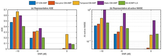
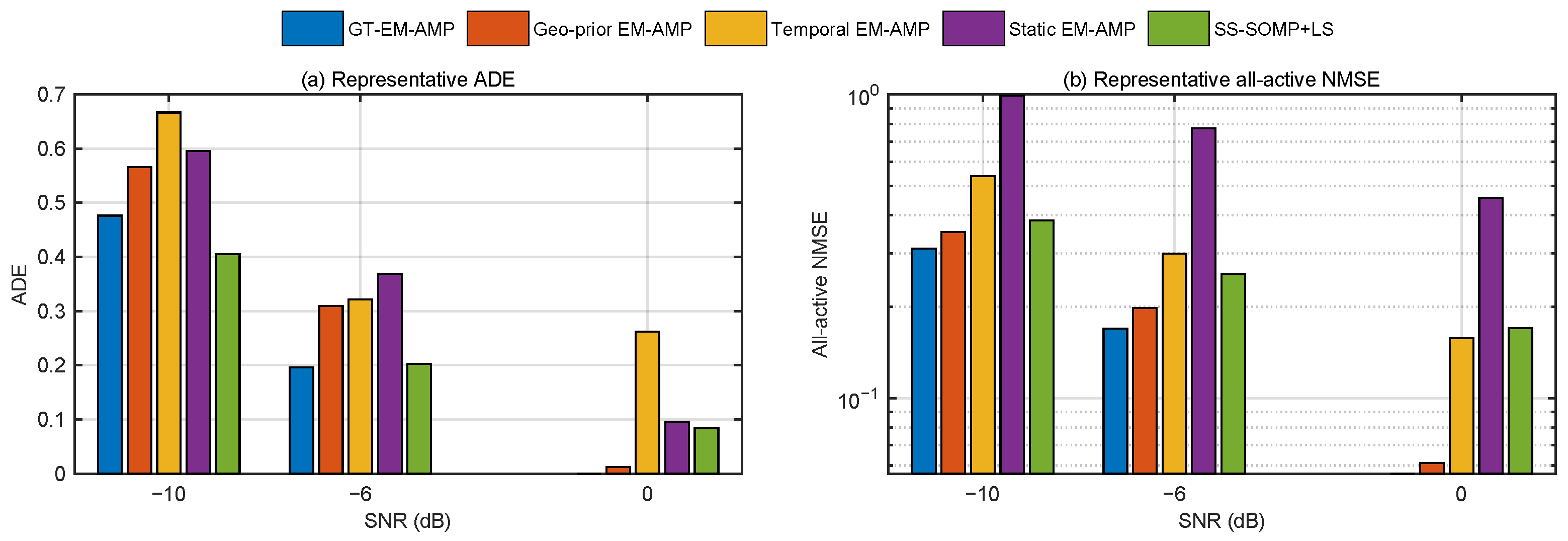
Figure 3 summarizes representative operating points at , , and 0 dB. These points compare the proposed prior-learning scheme with representative model-driven baselines, including frame-wise static, fixed-correlation temporal, geo-prior, and score-smoothed greedy alternatives. At 0 dB, GT-EM-AMP achieved zero median ADE and an all-active NMSE of 0.056. The corresponding all-active NMSE values were 0.061 for geo-prior EM-AMP, 0.157 for temporal EM-AMP, 0.457 for static EM-AMP, and 0.170 for SS-SOMP+LS. Geometry-only and temporal-only updates each improved performance, whereas their joint use achieved the most favorable detection–estimation tradeoff in the tested representative regime.
Figure 3.
Representative operating-point comparison of GT-EM-AMP, geo-prior EM-AMP, temporal EM-AMP, static EM-AMP, and SS-SOMP+LS under , , , , and at SNR values of , , and 0 dB. (a) Activity-detection error. (b) All-active NMSE over the true active rows, shown on a logarithmic scale. Lower values are better. The bars report the medians over the same 80 matched Monte Carlo trials used in Figure 2.
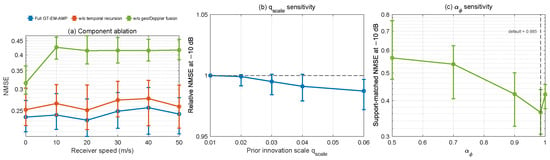
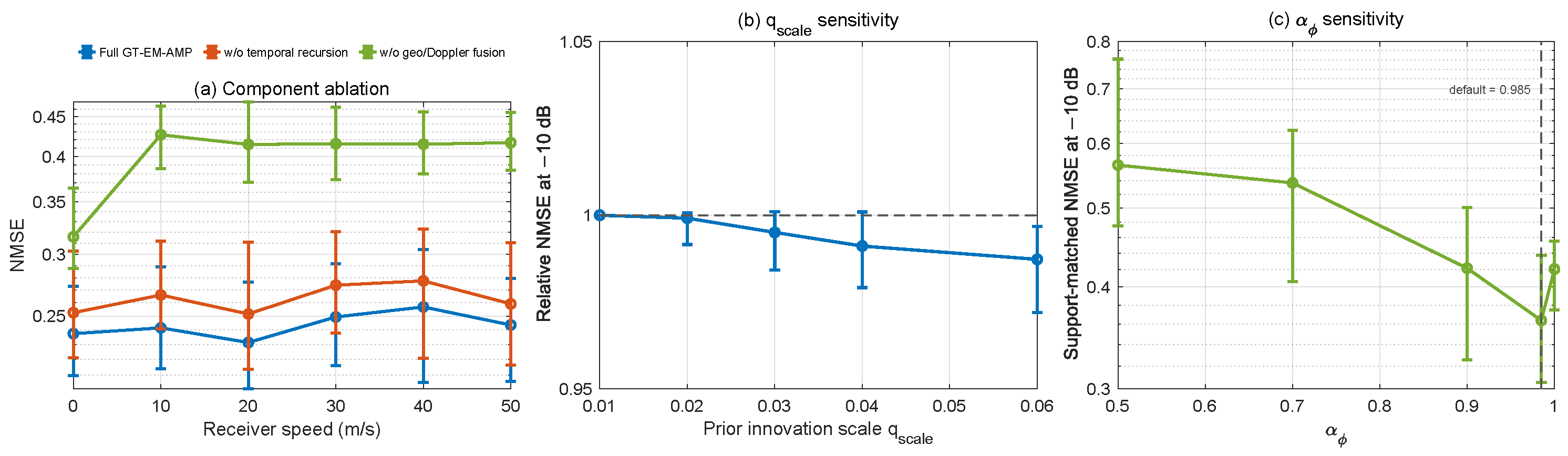
Figure 4 separates the contributions of temporal recursion and geo/Doppler-aware prior refinement. The “w/o temporal recursion” variant performs independent frame-wise estimation while retaining geometry-aided variance stabilization. The “w/o geo/Doppler fusion” variant retains fixed-correlation temporal recursion but removes the user-specific Doppler refinement and geometry-aware variance fusion. Full GT-EM-AMP combines both mechanisms. The sensitivity curve remains within a narrow range from 0.01 to 0.06, indicating that the prior recursion is not strongly affected by moderate changes in the innovation scale. Figure 4c further evaluates the variance-fusion coefficient . The lower NMSE values near support assigning the dominant weight to the EM-updated variance, while the selected value retains a small geometry-based correction.
Figure 4.
Component ablation and parameter sensitivity under , , , , , and SNR dB. (a) Support-matched NMSE versus receiver speed for the complete GT-EM-AMP scheme and two ablated variants. In panel (a), the “w/o temporal recursion” variant disables cross-frame prior propagation and reinitializes the prior independently for each frame while retaining the geometry-aware variance anchor. The “w/o geo/Doppler fusion” variant retains fixed-correlation temporal recursion but removes the user-specific Doppler refinement and geometry-aware variance fusion. All other parameters and support-selection rules are unchanged. (b) Relative support-matched NMSE under different prior innovation scales, normalized by the default . Panel (c) reports the support-matched NMSE versus ; the vertical dashed line marks the default value . Lower values are better. All panels use 40 matched Monte Carlo trials. Markers show the medians, and error bars show the interquartile ranges.
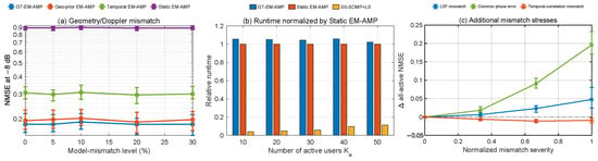
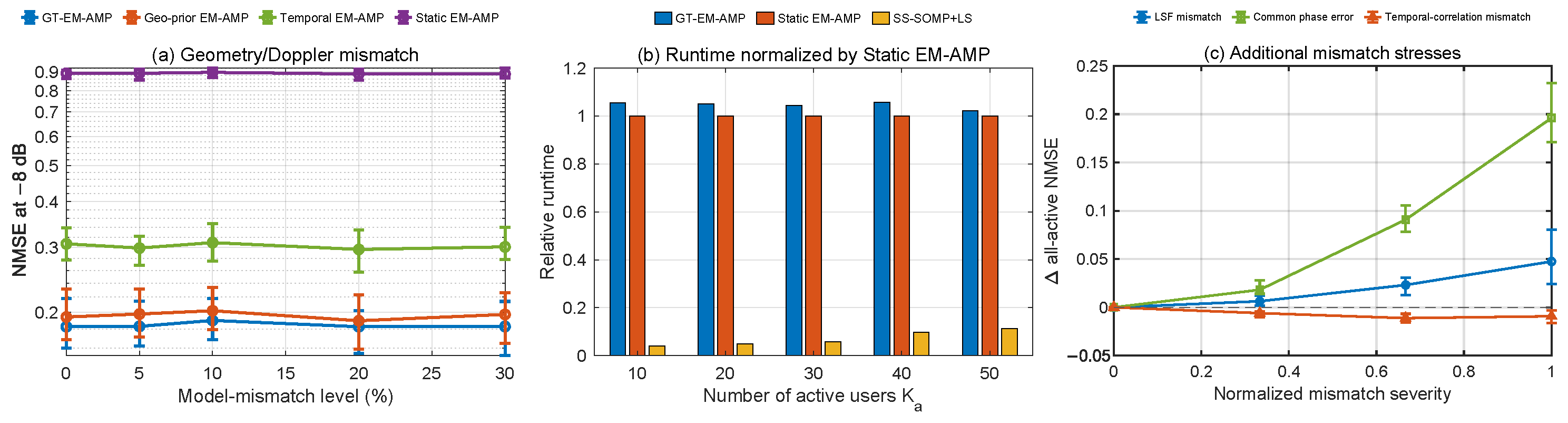
Figure 5 tests model mismatch and computational cost. In the mismatch experiment, the side information used by the prior update is perturbed before it is provided to the algorithm:
where and . The horizontal axis in Figure 5a denotes the standard-deviation-controlled mismatch level . GT-EM-AMP maintained lower NMSE than the temporal and static baselines across the tested mismatch levels. Geo-prior EM-AMP approached GT-EM-AMP at several mismatch levels, indicating that geometry-aware variance anchoring alone already contributes to variance stabilization. The additional cross-frame temporal recursion in GT-EM-AMP provided a more consistent detection–estimation tradeoff across the tested operating points. This behavior suggests that the geometry anchor mainly improves variance stability, whereas the temporal recursion provides additional continuity across consecutive pilot frames. The runtime experiment shows that the additional geo-temporal prior update introduced only a small overhead relative to frame-wise static EM-AMP as the number of active users increased. SS-SOMP+LS was faster, but Figure 2 and Figure 3 show that this lower cost was accompanied by weaker channel-estimation accuracy.
Figure 5.
Robustness and computational-cost evaluation. (a) Geometry/Doppler mismatch at SNR dB for GT-EM-AMP, geo-prior EM-AMP, temporal EM-AMP, and static EM-AMP. (b) Runtime normalized by static EM-AMP at SNR dB for GT-EM-AMP, static EM-AMP, and SS-SOMP+LS as increases from 10 to 50. (c) Change in all-active NMSE under large-scale-fading mismatch, common phase error, and temporal-correlation mismatch. Panels (a,b) use and ; panel (c) uses , , , , and . Panel (a) uses 80 matched trials, panel (b) uses 40 trials, and panel (c) uses 30 trials. Unless otherwise specified, the remaining parameters follow Table 2. In panels (a,c), markers show the median values and error bars show the interquartile ranges. In panel (c), the horizontal dashed line denotes zero NMSE change relative to the clean reference.
Figure 5c considers three additional controlled perturbations. The large-scale-fading (LSF) mismatch is implemented as
This controlled stress represents a common large-scale gain-calibration uncertainty rather than user-dependent shadow fading. The common phase error is introduced as
The temporal-correlation mismatch is generated by perturbing the effective Doppler according to
followed by recomputation of the Jakes-type correlation coefficient,
The four perturbation levels are mapped to the normalized coordinate , . The corresponding parameter levels are 0, 1, 2, and 4 dB for LSF mismatch; , , , and for common phase error; and 0, , , and for temporal-correlation mismatch. This common normalized axis facilitates visual comparison but does not imply equal physical severity across the three perturbation types. The vertical axis reports
where positive values indicate performance degradation caused by the perturbation. Under the selected perturbation ranges, common phase error produces the largest NMSE increase, whereas the effect of large-scale-fading mismatch grows more gradually with severity. The temporal-correlation mismatch produces negligible median degradation within the plotted uncertainty range over the considered short-frame setting.
3.1. Scalability Analysis
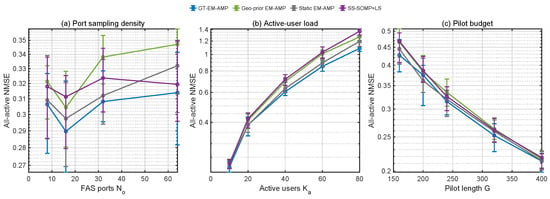
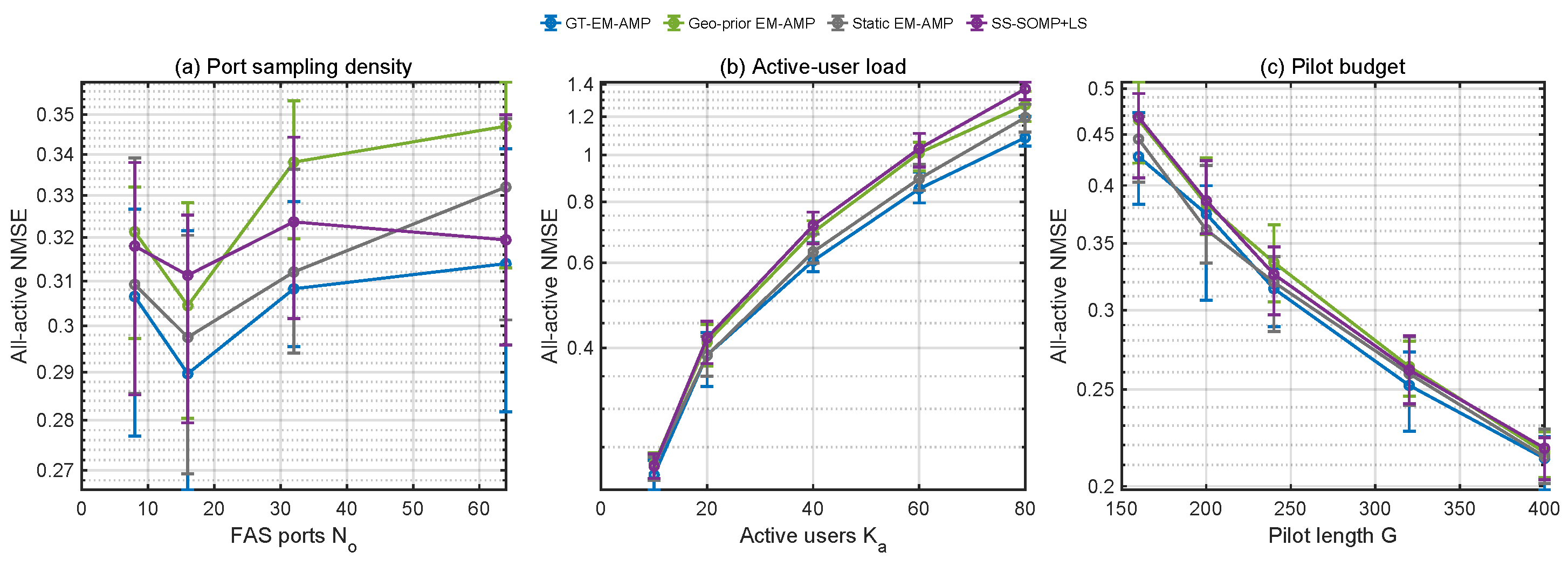
Figure 6 evaluates the effects of the number of FAS ports, the active-user load, and the pilot length. In Figure 6a, the physical aperture is fixed, so increasing only increases the port sampling density. The resulting NMSE varies within a relatively narrow range, consistent with the stronger correlation among densely spaced candidate ports. Figure 6b shows that the NMSE increases with because more active rows must be recovered from the same pilot observation. By contrast, Figure 6c shows a consistent improvement as G increases and more pilot measurements become available. GT-EM-AMP attains the lowest or near-lowest median NMSE over the reported operating points.
Figure 6.
Scalability comparison of GT-EM-AMP, geo-prior EM-AMP, static EM-AMP, and SS-SOMP+LS with respect to (a) FAS port sampling density, (b) active-user load, and (c) pilot length at SNR dB. Unless varied, , , , , and . The physical FAS aperture is fixed in panel (a), so increasing changes the candidate-port sampling density rather than the aperture length. Lower values are better. Markers show the medians over 40 matched Monte Carlo trials, and error bars show the interquartile ranges.
3.2. Nonuniform Receiver Mobility and Moving-User Robustness
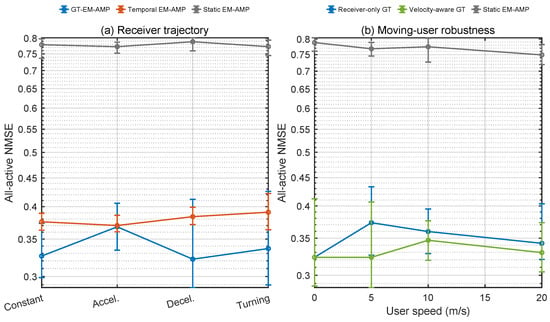
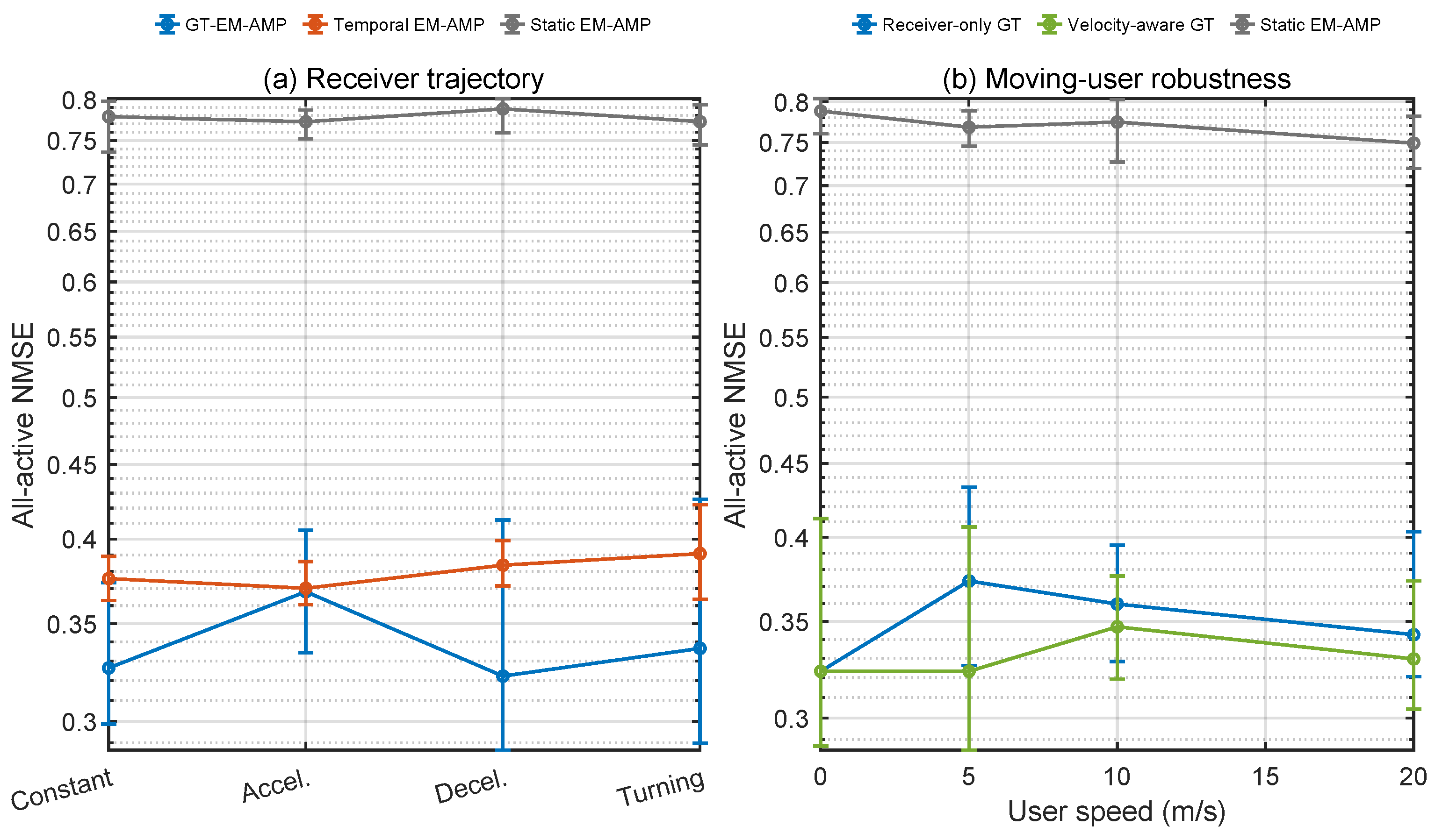
Figure 7 evaluates nonuniform receiver motion and moving users. The default experiments assume stationary access devices, whereas Figure 7b relaxes this assumption to examine moving-user robustness. Figure 7a shows that GT-EM-AMP achieves substantially lower all-active NMSE than static EM-AMP under all four receiver trajectories. Its performance is close to temporal EM-AMP under acceleration, while the advantage becomes more apparent under deceleration and turning. In Figure 7b, the receiver-only and velocity-aware variants coincide when the user speed is zero, which provides a consistency check for the two implementations. For moving users, incorporating the user velocity generally reduces the all-active NMSE. The receiver-only variant nevertheless maintains substantially lower all-active NMSE than static EM-AMP over the considered six-frame observation window.
Figure 7.
Nonuniform receiver mobility and moving-user robustness at SNR dB under , , , , , s, GHz, and m. (a) Absolute all-active NMSE for constant-velocity, acceleration, deceleration, and turning receiver trajectories. (b) Moving-user robustness for receiver-only GT, velocity-aware GT, and static EM-AMP as the user speed varies from 0 to 20 m/s. Receiver-only GT computes the Doppler prior using the receiver velocity while neglecting user motion, whereas velocity-aware GT uses the receiver–user relative velocity according to (11)–(14). Markers show the median all-active NMSE over 30 matched Monte Carlo trials, and error bars show the interquartile ranges. Detailed definitions of the receiver trajectories and moving-user configurations are provided in Supplementary Note S1.
Supplementary Figure S1 reports the paired NMSE changes relative to constant-velocity motion, while Supplementary Figure S2 shows the corresponding frame-wise transient behavior. Supplementary Table S1 summarizes the displacement and Doppler-mismatch diagnostics for the moving-user experiment.
3.3. Engineering Cost and Statistical Comparisons
Runtime measurements were obtained using the same MATLAB R2024b/Windows 11 workstation described above, without GPU acceleration. Table 4 summarizes the measured runtime, online state memory, and real-time factor. Relative to static EM-AMP, GT-EM-AMP increases the median frame runtime from 18.164 to 19.079 ms and requires an additional 0.714 MB of online state memory. The resulting real-time factor remains above one, so the current MATLAB CPU implementation does not meet the adopted 10 ms frame deadline. SS-SOMP+LS is substantially faster because it avoids iterative Bayesian updates, but its channel-estimation accuracy is lower in the SNR comparisons.
Table 4.
Engineering cost and real-time suitability at SNR dB, , , , , , and . Runtime/frame is reported as median [IQR] in milliseconds. RTF is computed relative to the 10 ms frame deadline; RTF values larger than one do not meet the adopted real-time target. ‘Iter.’ denotes the median number of AMP iterations per frame, and ‘Max-iter. frac.’ denotes the fraction of runs that reach . Memory denotes the measured online algorithm-state memory under the reported implementation and does not include the complete MATLAB process footprint.
Table 5 reports six prespecified paired comparisons based on matched Monte Carlo trials. For all-active NMSE, GT-EM-AMP outperforms geo-prior EM-AMP at , , and 0 dB, with Holm-adjusted p values below in all three comparisons. For ADE, SS-SOMP+LS performs better at dB, whereas GT-EM-AMP becomes favorable at and 0 dB. The paired analysis therefore confirms that the relative advantage depends on both SNR and metric: the geo-temporal prior provides a consistent channel-estimation gain, while the detection–estimation tradeoff changes in the very-low-SNR regime.
Table 5.
Prespecified paired statistical comparisons.
4. Discussion
The numerical results support viewing mobile FAS-GFRA CSI acquisition as a recursive support-and-channel inference problem. Temporal recursion and geometry-aware variance anchoring address complementary sources of uncertainty. The temporal predictor propagates the previous-frame posterior through the Doppler-dependent correlation and process innovation in (19), whereas the fusion in (41) regularizes the EM-updated variance toward a slower-varying geometry-dependent power scale. Their combination reduces dependence on either an inaccurate previous state or an unstable current-frame EM estimate. The ablation results are consistent with this interpretation: frame-wise geometry-aided estimation and fixed-correlation temporal recursion each provide partial gains, while Full GT-EM-AMP generally achieves the lowest median NMSE among the tested variants. Because the “w/o geo/Doppler fusion” variant removes both user-specific Doppler refinement and geometry-aware variance fusion, its degradation reflects their joint contribution.
At high SNR, the relative advantage of GT-EM-AMP narrows because the current-frame pilot observation becomes sufficiently informative for the geo-prior baseline to approach the proposed method. The unknown- screening results further indicate that the estimated activity probabilities can support cardinality-free detection at moderate SNR without threshold retuning. The known- results provide controlled comparisons under a common support-cardinality constraint.
The robustness and mobility studies further characterize the operating range of the physical prior. Figure 5a preserves the relative performance ordering over the tested geometry/Doppler mismatch range. Under the perturbation ranges considered in Figure 5c, common phase error produces the largest NMSE increase; however, this test represents a controlled phase offset rather than a complete synchronization model. Figure 7 and Supplementary Figures S1 and S2 extend the evaluation to acceleration, deceleration, turning, and moving users. GT-EM-AMP maintains lower all-active NMSE than static EM-AMP across the tested cases, and incorporating user velocity generally improves the moving-user result. These results demonstrate adaptation over the considered six-frame window, while longer-term nonstationarity and more general vehicular trajectories remain outside the present evaluation.
Estimation accuracy, runtime, memory, and side-information requirements have different units and application-dependent priorities. We therefore report them separately as a Pareto-style comparison, consistent with broader performance–complexity analyses [25]. Figure 6 characterizes estimation scalability with the FAS port density, active-user load, and pilot budget, while Table 4 reports runtime, memory, real-time factor, and side-information requirements. GT-EM-AMP retains the dominant per-iteration complexity and introduces modest additional runtime and state memory relative to static EM-AMP. SS-SOMP+LS provides a lower-cost operating point with weaker channel-estimation accuracy. The measured real-time factor of 1.91 also indicates that the current MATLAB CPU implementation does not meet the adopted 10 ms deadline.
The evaluation remains simulation-based and uses a controlled narrowband, short-horizon channel model with Jakes-type temporal correlation and coarse geometry/LSF side information. It does not include standardized spatially consistent vehicular channels, measured trajectories, channel measurements, or hardware-in-the-loop validation. Moreover, the mismatch studies isolate individual error sources, whereas geometry errors, Doppler-estimation errors, synchronization offsets, and channel nonstationarity may be coupled in practice. Practical geometry-to-power alignment should also rely on independent calibration or long-term channel statistics rather than simulation-generated realizations. Future work will consider standardized and measured vehicular channels, explicit synchronization, independent calibration, and GPU or hardware-parallel implementations. Hybrid physics- and data-driven predictors may also be useful when representative channel and trajectory data are available.
5. Conclusions
This article presented GT-EM-AMP for CSI acquisition in FAS-assisted GFRA with a mobile receiver. The method maps receiver trajectory and effective Doppler into a recursive Bernoulli–Gaussian prior and combines temporal prediction with a geometry-based variance anchor while preserving the scalar EM-AMP structure. The SNR comparisons show a favorable detection–estimation tradeoff, and the ablation results show that combining cross-frame temporal recursion, user-specific Doppler refinement, and geometry-aware variance fusion achieves the best performance among the tested variants. The mismatch, scalability, nonuniform-trajectory, and moving-user studies characterize the tested operating range, while paired comparisons support the reported channel-estimation gains and the SNR-dependent detection behavior. GT-EM-AMP retains the dominant complexity and adds modest runtime and memory relative to static EM-AMP, although the current MATLAB CPU implementation does not meet the 10 ms frame deadline. The present validation is limited to short-horizon simulations with coarse geometry information and a Jakes-type temporal model. Validation under standardized vehicular channels, measured trajectories, and hardware-in-the-loop platforms remains an important next step.
Supplementary Materials
The following supporting information can be downloaded at: https://www.mdpi.com/article/10.3390/electronics15132952/s1, Supplementary Note S1: mobility-scenario and Doppler-model definitions; Figure S1: paired change in all-active NMSE under nonuniform receiver trajectories; Figure S2: frame-wise all-active NMSE under acceleration and turning trajectories; Table S1: kinematic and Doppler diagnostics for the moving-user robustness experiment.
Author Contributions
Conceptualization, Y.S. and B.Z.; methodology, Y.S.; software, Y.S.; validation, Y.S.; formal analysis, Y.S.; investigation, Y.S.; writing—Original draft preparation, Y.S.; writing—Review and editing, S.C., X.C. and B.Z.; supervision, B.Z. All authors have read and agreed to the published version of the manuscript.
Funding
This research received no external funding.
Institutional Review Board Statement
Not applicable.
Informed Consent Statement
Not applicable.
Data Availability Statement
The simulation data and processed results presented in this study are available from the corresponding author upon reasonable request. The main simulation configurations are summarized in Table 2.
Conflicts of Interest
The authors declare no conflicts of interest.
Abbreviations
The following abbreviations are used in this manuscript:
| ADE | Activity-detection error |
| AMP | Approximate message passing |
| AoA | Angle of arrival |
| CSI | Channel state information |
| EM-AMP | Expectation-maximization approximate message passing |
| FAS | Fluid antenna system |
| GFRA | Grant-free random access |
| GT-EM-AMP | Geo-temporal expectation-maximization approximate message passing |
| IQR | Interquartile range |
| IoT | Internet of Things |
| LSFC | Large-scale fading coefficient |
| NMSE | Normalized mean square error |
| SOMP+LS | Simultaneous orthogonal matching pursuit with least squares |
| SS-SOMP+LS | Score-smoothed simultaneous orthogonal matching pursuit with least squares |
| WSSUS | Wide-sense stationary uncorrelated scattering |
References
- Choi, J.; Ding, J.; Le, N.-P.; Ding, Z. Grant-free random access in machine-type communication: Approaches and challenges. IEEE Wirel. Commun. 2022, 29, 151–158. [Google Scholar] [CrossRef] [Scilit]
- Chen, X.; Ng, D.W.K.; Yu, W.; Larsson, E.G.; Al-Dhahir, N.; Schober, R. Massive access for 5G and beyond. IEEE J. Sel. Areas Commun. 2021, 39, 615–637. [Google Scholar] [CrossRef] [Scilit]
- Zhang, Z.; Wong, K.-K.; Dang, J.; Zhang, Z.; Masouros, C.; Chae, C.-B. On fundamental limits of slow-fluid antenna multiple access for unsourced random access. IEEE Wirel. Commun. Lett. 2025, 14, 3455–3459. [Google Scholar] [CrossRef] [Scilit]
- Zhang, Z.; Wong, K.-K.; Dang, J.; Zhang, Z.; Chae, C.-B. On fundamental limits for fluid antenna-assisted integrated sensing and communications for unsourced random access. IEEE J. Sel. Areas Commun. 2026, 44, 136–149. [Google Scholar] [CrossRef] [Scilit]
- Zhang, Z.; Wong, K.-K.; Morales-Jimenez, D.; Jiang, H.; Ramirez-Espinosa, P.; Chae, C.-B.; Masouros, C. Finite-blocklength fluid antenna systems with spatial block-correlation channel model. IEEE Wirel. Commun. Lett. 2026, 15, 1911–1915. [Google Scholar] [CrossRef] [Scilit]
- Liu, L.; Yu, W. Massive connectivity with massive MIMO–Part I: Device activity detection and channel estimation. IEEE Trans. Signal Process. 2018, 66, 2933–2946. [Google Scholar] [CrossRef] [Scilit]
- Vila, J.P.; Schniter, P. Expectation-Maximization Gaussian-Mixture Approximate Message Passing. IEEE Trans. Signal Process. 2013, 61, 4658–4672. [Google Scholar] [CrossRef] [Scilit]
- Cheng, Y.; Liu, L.; Ping, L. Orthogonal AMP for massive access in channels with spatial and temporal correlations. IEEE J. Sel. Areas Commun. 2021, 39, 726–740. [Google Scholar] [CrossRef] [Scilit]
- Wong, K.-K.; Shojaeifard, A.; Tong, K.-F.; Zhang, Y. Fluid antenna systems. IEEE Trans. Wirel. Commun. 2021, 20, 1950–1962. [Google Scholar] [CrossRef] [Scilit]
- Wong, K.-K.; Tong, K.-F. Fluid antenna multiple access. IEEE Trans. Wirel. Commun. 2022, 21, 4801–4815. [Google Scholar] [CrossRef] [Scilit]
- Ramirez-Espinosa, P.; Morales-Jimenez, D.; Wong, K.-K. A new spatial block-correlation model for fluid antenna systems. IEEE Trans. Wirel. Commun. 2024, 23, 15829–15843. [Google Scholar] [CrossRef] [Scilit]
- Jiang, H.; Shi, W.; Chen, Z.; Zhang, Z.; Wong, K.-K.; Shin, H. Dynamic channel modeling of fluid antenna systems in UAV communications. IEEE Wirel. Commun. Lett. 2025, 14, 3169–3173. [Google Scholar] [CrossRef] [Scilit]
- Zeng, L.; Liao, X.; Ma, Z.; Zhang, R.; Niyato, D.; Jiang, H.; Wang, C.-X. Modeling and analysis of movable antenna aided MIMO wideband UAV-to-UAV channels for low-altitude economy networks. IEEE Trans. Wirel. Commun. 2026, 25, 10257–10273. [Google Scholar] [CrossRef] [Scilit]
- Jiang, H.; Shi, W.; Zhang, Z.; Pan, C.; Wu, Q.; Shu, F.; Liu, R.; Chen, Z.; Wang, J. Large-scale RIS enabled air-ground channels: Near-field modeling and analysis. IEEE Trans. Wirel. Commun. 2025, 24, 1074–1088. [Google Scholar] [CrossRef] [Scilit]
- Jiang, H.; Shi, W.; Chen, X.; Zhu, Q.; Chen, Z. High-efficient near-field channel characteristics analysis for large-scale MIMO communication systems. IEEE Internet Things J. 2025, 12, 7446–7458. [Google Scholar] [CrossRef] [Scilit]
- Zhang, Z.; Zhu, J.; Dai, L.; Heath, R.W. Successive Bayesian reconstructor for channel estimation in fluid antenna systems. IEEE Trans. Wirel. Commun. 2025, 24, 1992–2006. [Google Scholar] [CrossRef] [Scilit]
- Zhang, Z.; Morales-Jimenez, D.; Dang, J.; Zhang, Z.; Masouros, C.; Jiang, H. Low-complexity CSI acquisition exploiting geographical diversity in fluid antenna system. arXiv 2025, arXiv:2509.08598. [Google Scholar] [CrossRef] [Scilit]
- Zhang, Z.; Dang, J.; Morales-Jimenez, D.; Jiang, H.; Zhang, Z.; Masouros, C.; Chae, C.-B. Joint activity detection and channel estimation for fluid antenna system exploiting geographical and angular information. IEEE J. Sel. Top. Signal Process. 2026, 20, 354–370. [Google Scholar] [CrossRef] [Scilit]
- Zhang, Z.; Wong, K.-K.; Jiang, H.; Masouros, C.; Chae, C.-B. Cramér–Rao bounds for activity detection in conventional and fluid antenna systems. IEEE Wirel. Commun. Lett. 2026, 15, 3059–3063. [Google Scholar] [CrossRef] [Scilit]
- Wu, Y.; Zhang, Z.; Jiang, H.; Wong, K.-K.; Chae, C.-B. Learned-approximate message passing under Karhunen–Loeve modeling for fluid antenna systems. IEEE Wirel. Commun. Lett. 2026, 15, 2719–2723. [Google Scholar] [CrossRef] [Scilit]
- Ziniel, J.; Schniter, P. Dynamic compressive sensing of time-varying signals via approximate message passing. IEEE Trans. Signal Process. 2013, 61, 5270–5284. [Google Scholar] [CrossRef] [Scilit]
- Zhang, Z.; Rao, B.D. Sparse signal recovery with temporally correlated source vectors using sparse Bayesian learning. IEEE J. Sel. Top. Signal Process. 2011, 5, 912–926. [Google Scholar] [CrossRef] [Scilit]
- Zhu, W.; Tao, M.; Yuan, X.; Guan, Y. Message passing-based joint user activity detection and channel estimation for temporally-correlated massive access. IEEE Trans. Commun. 2023, 71, 3576–3591. [Google Scholar] [CrossRef] [Scilit]
- Tropp, J.A.; Gilbert, A.C.; Strauss, M.J. Algorithms for simultaneous sparse approximation. Part I: Greedy pursuit. Signal Process. 2006, 86, 572–588. [Google Scholar] [CrossRef] [Scilit]
- Miuccio, L.; Panno, D.; Riolo, S. A Flexible Encoding/Decoding Procedure for 6G SCMA Wireless Networks via Adversarial Machine Learning Techniques. IEEE Trans. Veh. Technol. 2023, 72, 3288–3303. [Google Scholar] [CrossRef] [Scilit]

Disclaimer/Publisher’s Note: The statements, opinions and data contained in all publications are solely those of the individual author(s) and contributor(s) and not of MDPI and/or the editor(s). MDPI and/or the editor(s) disclaim responsibility for any injury to people or property resulting from any ideas, methods, instructions or products referred to in the content. |
© 2026 by the authors. Licensee MDPI, Basel, Switzerland. This article is an open access article distributed under the terms and conditions of the Creative Commons Attribution (CC BY) license.