Adaptive Neural Network Preset-Time Control for RDDV with Unknown Dynamics

Abstract

This paper addresses the high-precision position tracking control problem for the rotary direct-drive valve (RDDV) subject to complex nonlinear dynamics and unknown external disturbances. To achieve superior transient and steady-state performance, a novel adaptive neural network preset-time control (ANNPTC) strategy is proposed. Distinct from conventional finite-time or fixed-time control schemes, the proposed ANNPTC ensures that the tracking error converges to a prescribed neighborhood of the origin within a prescribed residual set after the user-defined time $T_c$ under the admissible initial condition. Specifically, adaptive radial basis function neural networks (RBFNNs) are utilized to estimate and compensate for unmodeled dynamics and disturbances, significantly enhancing the steady-state precision of the system. The uniform ultimate boundedness of all signals in the closed-loop system and the prescribed-performance property are established via Lyapunov stability analysis. Finally, extensive simulation results on a high-fidelity RDDV model demonstrate that the proposed method yields faster response speed and higher tracking accuracy compared with benchmark controllers, thereby validating its efficacy and superiority in RDDV applications.

1. Introduction

The rotary direct-drive servo valve (RDDV) offers significant advantages over traditional proportional and servo valves, including compact structural design, rapid transient response, enhanced reliability, superior anti-contamination capability, and high power density [1,2,3,4,5]. These attributes render RDDV highly promising for applications in precision machining, aircraft braking systems, and specialized robotics. By employing a rotary drive mechanism, the RDDV directly converts the electromagnetic motor’s rotation into the linear displacement of the valve spool. This direct-drive architecture eliminates the hydraulic pilot stage (pre-stage amplification) found in conventional valves, thereby fundamentally improving system reliability and robustness against fluid contamination. Furthermore, the direct-drive configuration allows the RDDV to respond effectively to control signals, facilitating the implementation of advanced control algorithms to enhance both transient and steady-state tracking precision [6,7].

However, the transition from conventional hydraulic valves to RDDV introduces significant challenges, such as modeling complexities, intensified nonlinearities, unknown dynamic disturbances, and high-frequency interference, all of which can severely degrade control performance [8,9,10]. To mitigate these issues, early researchers explored various strategies ranging from traditional PID control to adaptive active disturbance rejection control (ADRC) [11], achieving notable success. Nevertheless, prior studies have predominantly focused on steady-state convergence. For high-bandwidth RDDV, there are stringent requirements for transient performance and settling time. Within current control theory, finite-time control [12,13,14] ensures faster convergence than asymptotic methods, but its settling time is heavily dependent on the system’s initial conditions. Fixed-time control [15,16,17] addresses this limitation, yet the upper bound of the convergence time remains a complex function of controller parameters, making it difficult to pre-configure for practical engineering constraints. Recently, preset-time control (PTC) [18,19,20] has gained traction as it allows designers to explicitly define the convergence time $T_c$ according to task requirements, which is critical for the high-frequency switching and synchronization of RDDV. Given the complex nonlinear dynamics and unknown disturbances inherent in RDDV systems, a singular PTC framework is often insufficient. Consequently, this study incorporates adaptive neural network (ANN) technology [21,22,23] to approximate unknown system dynamics. For RDDV systems, the uncertain dynamics are not only caused by parameter perturbations but also by nonlinear friction, hydraulic flow-force variation, eccentric-transmission coupling, radial hydraulic imbalance, and unmodeled electrical dynamics. These uncertainties are difficult to describe accurately using a fixed parametric model. Therefore, an adaptive approximation mechanism is required to reconstruct the lumped nonlinear dynamics online. Among intelligent approximation methods, the RBFNN is suitable for this task because of its local approximation capability, simple linear-in-parameter structure, and convenient integration with Lyapunov-based adaptive laws. In the proposed controller, the RBFNN is not used as an independent black-box controller; instead, it is embedded into the backstepping control structure as an adaptive compensation term for the unknown dynamics. The overall control law consists of nominal model compensation, RBFNN-based adaptive compensation, preset-time performance regulation, and recursive stabilization terms. This structure enables the controller to retain a clear physical interpretation while improving robustness against nonlinear uncertainties and parameter variations. The proposed scheme utilizes RBFNN to reconstruct the unknown nonlinear mappings of RDDV dynamics online without requiring a priori structural information. By integrating neural-network-based intelligent compensation with a preset-time performance function [24,25,26], the controller effectively counteracts unmodeled disturbances in real-time. This ensures that tracking errors remain within predefined performance bounds even under severe operating conditions and parameter variations, thereby significantly enhancing system robustness. The primary contributions of this paper are summarized as follows:

• Mathematical Modeling of RDDV: A comprehensive mathematical model of the rotary direct-drive servo valve is established. The model explicitly incorporates quantifiable nonlinear dynamics and disturbances, while unmodeled, time-varying dynamic uncertainties are represented implicitly within the formulation.
• Novel ANNPTC Framework: To meet the requirements for a high transient response, an adaptive neural network preset-time control (ANNPTC) framework is proposed. Under the admissible initial condition $|s_1\left(0\right)|<{\rho }_0$, the proposed method ensures that the spool displacement tracking error remains within the prescribed-performance boundary and enters a predefined residual set after the user-specified time $T_c$, thereby achieving uniform ultimate boundedness of the closed-loop signals.
• Online Adaptive Compensation: Leveraging the universal approximation properties of radial basis function (RBF) neural networks, an online adaptive weight update law is designed. This mechanism achieves real-time compensation of strong nonlinear disturbances and parameter uncertainties, including flow forces, nonlinear friction, and unmodeled dynamics, without requiring precise knowledge of the system’s structural dynamics, thereby significantly improving robust stability.

The remainder of this paper is organized as follows. Section 2 establishes the refined electromechanical–hydraulic model of the RDDV and derives the control-oriented strict-feedback representation. Section 3 presents the ANNPTC design, including the preset-time performance function, RBFNN approximation, adaptive laws, and stability analysis. Section 4 provides comparative simulations and sensitivity analyses to verify the tracking performance and robustness of the proposed method. Finally, Section 5 concludes the paper and discusses future experimental work.

2. Establishment of the RDDV Model

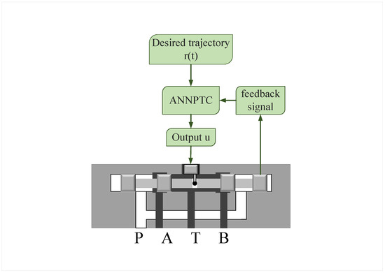
The RDDV is a typical electromechanical–hydraulic coupled system, in which the input voltage is first converted into the electromagnetic torque of the limited-angle torque motor, and then the rotational motion of the motor is transformed into the translational motion of the spool through the eccentric ball-pair mechanism. During this process, the spool motion is affected by the motor dynamics, nonlinear transmission geometry, hydraulic flow force, friction, radial hydraulic imbalance, and unmodeled external disturbances. A schematic diagram of the RDDV structure is shown in Figure 1 below. Therefore, a refined mathematical model is established in this section to reveal the dominant physical characteristics of the RDDV and to provide a reasonable basis for the subsequent controller design [2,7,27].

Figure 1. Simplified structural diagram of RDDV.

Let u, i, $\theta$, and $\omega$ denote the motor input voltage, coil current, angular displacement, and angular velocity, respectively. The electrical dynamics of the limited-angle torque motor can be described as

$$u=R_{m}i+L_m\dot{i}+K_e\omega ,$$

(1)

where $R_m$ is the coil resistance, $L_m$ is the coil inductance, and $K_e$ is the back electromotive force coefficient. The electromagnetic torque generated by the motor is given by

$$T_e=K_{t}i,$$

(2)

where $K_t$ is the torque coefficient. Considering the load torque caused by the spool motion and hydraulic forces, the rotational dynamics of the motor are expressed as

$$J_r\dot{\omega }+B_r\omega +T_{\ell }=K_{t}i+{\Delta }_r\left(t\right),$$

(3)

where $J_r$ is the equivalent rotational inertia, $B_r$ is the equivalent rotational damping coefficient, $T_{\ell }$ is the load torque acting on the motor shaft, and ${\Delta }_r\left(t\right)$ represents the motor-side lumped uncertainty, including torque ripple, amplifier dynamics, assembly error, and parameter perturbations.

The eccentric ball-pair mechanism establishes a nonlinear geometric relationship between the motor angular displacement and the spool displacement. Denoting the spool displacement by $x_v$ and the eccentricity of the ball-pair mechanism by $e_b$, one has

$$x_v=e_{b}sin\theta .$$

(4)

In the subsequent control-oriented derivation, the valve is assumed to operate in the normal limited-angle region satisfying $|x_v| < e_b$ and $cos\theta > 0$. Under this standard local operating condition, the mapping between $\theta$ and $x_v$ is single-valued and nonsingular. Accordingly, the spool velocity and acceleration are obtained as

$${\dot{x}}_v=e_{b}cos\theta \dot{\theta },$$

(5)

and

$${\ddot{x}}_v=e_{b}cos\theta \ddot{\theta }-e_{b}sin\theta {\dot{\theta }}^2.$$

(6)

It can be observed from (6) that the eccentric transmission introduces an inherent geometric nonlinearity. In particular, the term $-e_{b}sin\theta {\dot{\theta }}^2$ reflects the nonlinear acceleration component induced by the rotational motion of the motor. This effect becomes non-negligible when the valve operates under high-frequency tracking conditions.

The axial dynamics of the spool [6] can be written as

$$m_s{\ddot{x}}_v+c_s{\dot{x}}_v+k_s{x}_v+F_{\mu }(x_v,{\dot{x}}_v)+F_h(x_v,p_s,p_L)+F_c(x_v,{\dot{x}}_v,p_L,t)=F_a+{\Delta }_s\left(t\right),$$

(7)

where $m_s$ is the equivalent mass of the spool and the entrained oil, $c_s$ is the viscous damping coefficient, and $k_s$ is the equivalent mechanical-hydraulic stiffness. $F_{\mu }(x_v,{\dot{x}}_v)$ denotes the nonlinear friction force, $F_h(x_v,p_s,p_L)$ denotes the hydraulic flow force, where $p_s$ and $p_L$ are regarded as bounded time-varying hydraulic variables, and $F_c(x_v,{\dot{x}}_v,p_L,t)$ represents the complex force caused by eccentric transmission, radial hydraulic imbalance, spool tilting, and possible contact between the spool shoulder and sleeve. $F_a$ is the axial driving force generated by the eccentric ball-pair mechanism, and ${\Delta }_s\left(t\right)$ denotes external disturbances and unmodeled spool-side dynamics.

For a more explicit description of the velocity-dependent friction effect, the nonlinear friction force can be represented in a Stribeck-like form [28,29,30]:

$$F_{\mu }(x_v,{\dot{x}}_v)=c_f{\dot{x}}_v+\left[F_C+(F_S-F_C)exp\left(-{\left|{\displaystyle \frac{{\dot{x}}_v}{v_S}}\right|}^2\right)\right]sgn\left({\dot{x}}_v\right),$$

(8)

where $c_f$ is the local viscous friction coefficient, $F_C$ is the Coulomb friction force, $F_S$ is the maximum static friction force, and $v_S$ is the Stribeck velocity. The term $c_s{\dot{x}}_v$ in (7) represents the nominal linear damping retained in the model, whereas $c_f{\dot{x}}_v$ and the remaining nonlinear friction components are treated as uncertain friction effects. Since these friction parameters are difficult to identify accurately and may vary with temperature, oil contamination, and mechanical wear, the uncertain part of $F_{\mu }$ is treated as an unknown nonlinear dynamic term in the subsequent control design.

The load flow through the throttling window can be described by the orifice equation

$$Q_L=C_d{A}_v\left(x_v\right)\sqrt{{\displaystyle \frac{2}{{\rho }_o}}\Delta p},$$

(9)

where $C_d$ is the discharge coefficient, $A_v\left(x_v\right)$ is the effective throttling area, ${\rho }_o$ is the oil density, and $\Delta p$ is the pressure drop across the valve orifice. Equation (9) is used for the local positive-opening operating region, in which the pressure-drop direction is fixed and $\Delta p>0$. When bidirectional flow is considered, the corresponding signed orifice equation should be used instead. For the micro-flow RDDV with a non-full-circumference throttling window, the effective throttling area can be locally approximated as

$$A_v\left(x_v\right)=w_v{x}_v,$$

(10)

where $w_v$ denotes the equivalent width of the throttling window and $x_v$ denotes the local positive spool opening. The corresponding steady-state flow force is generally expressed as

$$F_h(x_v,p_s,p_L)=C_h{A}_v\left(x_v\right)\Delta pcos{\varphi }_h,$$

(11)

where $C_h$ is the flow-force coefficient and ${\varphi }_h$ is the jet angle. In practical operation, $C_h$, $\Delta p$, and ${\varphi }_h$ are influenced by the spool opening, supply pressure fluctuation, oil temperature, and internal flow pattern. Therefore, the exact hydraulic force is difficult to obtain, and its uncertain component is also included in the lumped unknown dynamics.

Based on the above analysis, the refined RDDV model contains both explicitly modeled physical dynamics and implicitly represented unknown dynamics. The explicitly modeled part describes the dominant electromechanical–hydraulic coupling mechanism, while the unknown part accounts for nonlinear friction, flow-force uncertainty, radial hydraulic imbalance, sticking-related dynamics, parameter variations, and external disturbances. This modeling strategy avoids excessive dependence on inaccurate physical parameters and provides a practical foundation for the adaptive neural network preset-time controller developed in the following section.

3. Adaptive Neural Network Preset-Time Control Design

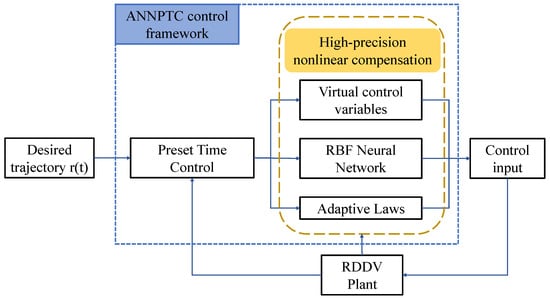
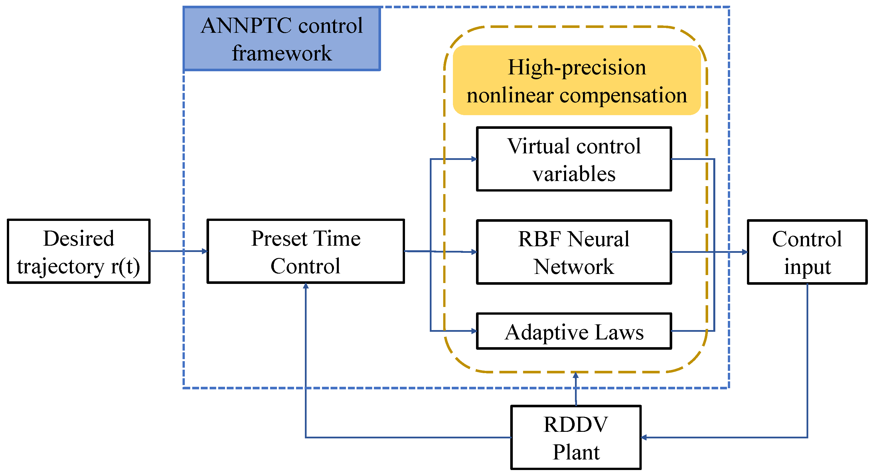
In this section, an adaptive neural network preset-time prescribed-performance control scheme is developed for the RDDV system. The preset-time performance function is employed to specify the time at which the allowable tracking-error boundary reaches its final residual value, while RBF neural networks are used to approximate the lumped unknown dynamics caused by nonlinear friction, flow-force uncertainty, eccentric-transmission coupling, and unmodeled disturbances. Based on these methods, a recursive backstepping controller is designed, and its uniformly ultimately bounded stability together with the prescribed tracking-error constraint is analyzed. The design framework for the control algorithm proposed in this paper is shown in Figure 2 below.

Figure 2. Design framework for the adaptive neural network preset-time control.

3.1. Preset-Time Performance Function

Let $r\left(t\right)$ be the desired spool displacement trajectory, and define the tracking error as

$$s_1={\chi }_1-r.$$

(12)

The preset-time performance boundary is selected as

$$\rho \left(t\right)=\left\{\begin{array}{cc}({\rho }_0-{\rho }_{\infty }){\left(1-{\displaystyle \frac{t}{T_c}}\right)}^{\ell }+{\rho }_{\infty },\hfill & 0\le t<T_c,\hfill \\ {\rho }_{\infty },\hfill & t\ge T_c,\hfill \end{array}\right.$$

(13)

where ${\rho }_0>{\rho }_{\infty }>0$, $T_c>0$ is the user-defined convergence time, and $\ell >3$ is a shaping parameter selected to provide the smooth derivatives required by the backstepping controller. If

$$|s_1\left(t\right)|<\rho \left(t\right),$$

(14)

then the tracking error satisfies $|s_1\left(t\right)|<{\rho }_{\infty }$ for all $t\ge T_c$. For the subsequent Lyapunov design, define

$$\pi ={\displaystyle \frac{s_1}{{\rho }^2\left(t\right)-s_1^2}}.$$

(15)

It is assumed that $|s_1\left(0\right)|<{\rho }_0$.

3.2. RBF Neural Network Approximation

For any continuous unknown nonlinear function $\Omega \left(\zeta \right)$ defined on a compact set, the RBF neural network approximation is written as

$$\Omega \left(\zeta \right)={\Theta }^{*T}\phi \left(\zeta \right)+\epsilon \left(\zeta \right),\left|\epsilon \left(\zeta \right)\right|\le \overline{\epsilon },$$

(16)

where ${\Theta }^{*}$ is the ideal weight vector, $\phi \left(\zeta \right)$ is the RBF basis vector, and $\epsilon \left(\zeta \right)$ is the bounded approximation error. The Gaussian function is adopted as the activation function of each RBF node, which is expressed as

$${\phi }_j\left(\zeta \right)=exp\left(-{\displaystyle \frac{\parallel \zeta -c_j{\parallel }^2}{{\sigma }_j^2}}\right),j=1,2,\dots ,N,$$

(17)

where $c_j$ and ${\sigma }_j$ denote the center and width of the jth Gaussian basis function, respectively, and N is the number of neural nodes. The Gaussian activation function provides localized nonlinear mapping capability, enabling the RBFNN to approximate the unknown dynamics with different local characteristics over the compact operating region.

For the RDDV model, the lumped unknown dynamics are approximated by

$${\Omega }_2({\chi }_{\left[2\right]},t)={\Theta }_2^{*T}{\phi }_2\left({\zeta }_2\right)+{\epsilon }_2,{\Omega }_3(\chi ,t)={\Theta }_3^{*T}{\phi }_3\left({\zeta }_3\right)+{\epsilon }_3,$$

(18)

where ${\zeta }_2={\chi }_{\left[2\right]}$, ${\zeta }_3=\chi$, and $|{\epsilon }_i| \le {\overline{\epsilon }}_i$, $i=2,3$. The bounded errors ${\epsilon }_i$ include the RBF approximation errors and the bounded residual time-varying components that cannot be represented by the selected state-dependent basis functions. The corresponding estimates and weight estimation errors are defined as

$${\widehat{\Omega }}_i={\widehat{\Theta }}_i^T{\phi }_i\left({\zeta }_i\right),{\tilde{\Theta }}_i={\Theta }_i^{*}-{\widehat{\Theta }}_i,i=2,3.$$

(19)

In implementation, the RBFNN inputs are normalized before being sent to the Gaussian basis functions. After normalization, each variable approximately lies in the interval $[-1,1]$. The RBF centers are selected according to the compact operating region of the RDDV states. Specifically, the measurable state variables are first limited to their normal working intervals and then normalized to comparable numerical ranges. The centers $c_j$ are uniformly distributed over the normalized compact domain, and the width ${\sigma }_j$ is selected according to the distance between adjacent centers so that neighboring Gaussian functions have sufficient overlap. This choice provides continuous coverage of the operating region while avoiding excessive numerical sensitivity. During the simulation, the centers and widths are kept fixed, whereas only the neural weights are updated online by the adaptive laws.

3.3. The Design of ANNPTC

According to the refined RDDV model established in Section 2, the input voltage u first determines the motor current through the electrical dynamics (1), and the motor current further generates the electromagnetic torque through (2). The torque transmission process is reflected in the spool axial dynamics (7) through the equivalent driving force $F_a$, while the nonlinear geometric relationship between the motor angle and the spool displacement is described by (4)–(6). Therefore, for controller synthesis, the dominant current-to-acceleration channel is extracted as a nominal positive gain, and the remaining motor inertia, load-torque variation, nonlinear transmission terms, hydraulic-force uncertainty, and unmodeled disturbances are collected into lumped unknown dynamics. Under Assumption 1, the RDDV is rewritten as the following third-order control-oriented strict-feedback system.

Define the state variables as

$${\chi }_1=x_v,{\chi }_2={\dot{x}}_v,{\chi }_3=i,$$

(20)

where ${\chi }_1$ denotes the spool displacement, ${\chi }_2$ denotes the spool velocity, and ${\chi }_3$ denotes the motor coil current. From (1) and (7), the RDDV dynamics can be organized into the following strict-feedback form:

$$\begin{array}{cc}\hfill {\dot{\chi }}_1& ={\chi }_2,\hfill \\ \hfill {\dot{\chi }}_2& ={\mathcal{F}}_2({\chi }_{\left[2\right]},t)+b_m{\chi }_3+{\Omega }_2({\chi }_{\left[2\right]},t),\hfill \\ \hfill {\dot{\chi }}_3& ={\mathcal{F}}_3(\chi ,t)+b_{e}u+{\Omega }_3(\chi ,t),\hfill \end{array}$$

(21)

where

$${\chi }_{\left[2\right]}={[{\chi }_1,{\chi }_2]}^T,\chi ={[{\chi }_1,{\chi }_2,{\chi }_3]}^T.$$

(22)

In (21), $b_m>0$ denotes the nominal equivalent gain from the motor current to the spool acceleration, which represents the dominant torque-generation and eccentric-transmission effect described by (2)–(7). The exact gain may vary with the transmission geometry and hydraulic load; such variation is included in ${\Omega }_2({\chi }_{\left[2\right]},t)$. Meanwhile, $b_e=1/L_m>0$ is the nominal voltage-to-current gain derived from the motor electrical Equation (1). To distinguish the model-based compensation terms from the uncertain dynamics, the known parts of the mechanical-hydraulic and electrical channels are defined as

$${\mathcal{F}}_2({\chi }_{\left[2\right]},t)=-{\displaystyle \frac{c_s}{m_s}}{\chi }_2-{\displaystyle \frac{k_s}{m_s}}{\chi }_1-{\displaystyle \frac{1}{m_s}}{\overline{F}}_h({\chi }_1,p_s,p_L),$$

(23)

and

$${\mathcal{F}}_3(\chi ,t)=-{\displaystyle \frac{R_m}{L_m}}{\chi }_3-{\displaystyle \frac{K_e}{L_m}}\omega ,\omega ={\omega }_v({\chi }_1,{\chi }_2)={\displaystyle \frac{{\chi }_2}{e_{b}cos\left(arcsin({\chi }_1/e_b)\right)}}.$$

(24)

where ${\overline{F}}_h({\chi }_1,p_s,p_L)$ is the nominal part of the hydraulic flow force in (11). The expression of $\omega$ follows from (5) and is well defined in the nonsingular operating region specified in Assumption 1. Therefore, ${\mathcal{F}}_2({\chi }_{\left[2\right]},t)$ mainly contains the nominal damping, stiffness, and flow-force terms in the spool dynamics, while ${\mathcal{F}}_3(\chi ,t)$ contains the nominal resistance and back electromotive force terms in the current dynamics, where $\omega$ can be expressed as a nonlinear function of ${\chi }_1$ and ${\chi }_2$. These known dynamics will be directly compensated by feedforward terms in the controller.

The remaining uncertain terms are collected into ${\Omega }_2({\chi }_{\left[2\right]},t)$ and ${\Omega }_3(\chi ,t)$. According to the spool dynamics (7), the mechanical-hydraulic unknown dynamics are expressed as

$${\Omega }_2({\chi }_{\left[2\right]},t)={\displaystyle \frac{1}{m_s}}\left[\Delta F_a-F_{\mu }({\chi }_1,{\chi }_2)-\Delta F_h({\chi }_1,p_s,p_L)-F_c({\chi }_1,{\chi }_2,p_L,t)+{\Delta }_s\left(t\right)\right],$$

(25)

where $\Delta F_a$ denotes the uncertainty of the eccentric-transmission driving force after extracting the nominal current-related term $m_s{b}_m{\chi }_3$, and $\Delta F_h=F_h-{\overline{F}}_h$ denotes the uncertain component of the hydraulic flow force. Similarly, based on (1), the electrical unknown dynamics are written as

$${\Omega }_3(\chi ,t)={\Delta }_e(\chi ,t),$$

(26)

where ${\Delta }_e(\chi ,t)$ represents the lumped electrical uncertainty, including parameter perturbations, amplifier dynamics, unmodeled back electromotive force variation, and current channel disturbances. The unknown functions ${\Omega }_2({\chi }_{\left[2\right]},t)$ and ${\Omega }_3(\chi ,t)$ are approximated online by the RBFNNs defined in Section 3.2. The control objective is to design the voltage input u such that ${\chi }_1$ tracks the desired spool displacement $r\left(t\right)$ within the preset-time performance boundary.

It should be emphasized that the strict-feedback model used for controller synthesis is a control-oriented local representation of the RDDV rather than a global exact model over all possible mechanical positions. The RDDV is considered to operate in the normal limited-angle working region, where $|x_v| < e_b$, $cos\theta >0$, and the transmission direction of the eccentric ball-pair mechanism does not change. Under this condition, the mapping from motor rotation to spool translation is single-valued and nonsingular, and the dominant current-to-spool-acceleration channel keeps a fixed positive sign. Therefore, the nominal gain $b_m$ can be selected as a positive constant. The variations caused by eccentric-transmission nonlinearity, flow-force uncertainty, nonlinear friction, radial hydraulic imbalance, and parameter perturbations are not ignored; instead, they are collected into the lumped unknown function ${\Omega }_2({\chi }_{\left[2\right]},t)$ and compensated online by the RBFNN. Similarly, the electrical gain $b_e=1/L_m$ is positive because the motor inductance satisfies $L_m>0$, while the unmodeled amplifier dynamics and electrical parameter variations are included in ${\Omega }_3(\chi ,t)$. Hence, the strict-feedback form is valid within the compact admissible operating region considered in this work.

Assumption 1. 

The desired trajectory $r\left(t\right)$ and the derivatives required by the backstepping design are bounded. The RDDV operates in a compact normal working region where $|{\chi }_1| < e_b$, $cos\theta >0$, and the nominal input gains $b_m>0$ and $b_e=1/L_m>0$ are known. The lumped unknown dynamics are continuous with respect to the measurable states and have bounded residual time-varying components on this compact region.

Step 1: Let the spool displacement tracking error be

$$s_1={\chi }_1-r.$$

(27)

To incorporate the preset-time performance constraint, consider the barrier Lyapunov function

$$V_1={\displaystyle \frac{1}{2}}ln\left({\displaystyle \frac{{\rho }^2\left(t\right)}{{\rho }^2\left(t\right)-s_1^2}}\right),$$

(28)

where $\rho \left(t\right)$ is the preset-time performance boundary defined in (13). As $|s_1|$ approaches $\rho \left(t\right)$, the function tends to infinity. Therefore, the boundedness of $V_1$ guarantees that the tracking error cannot reach the prescribed boundary.

Differentiating (28) gives

$${\dot{V}}_1=\pi \left({\dot{s}}_1-{\displaystyle \frac{\dot{\rho }}{\rho }}{s}_1\right),$$

(29)

where

$$\pi ={\displaystyle \frac{s_1}{{\rho }^2\left(t\right)-s_1^2}}.$$

(30)

Moreover, since $-ln(1-y)\le y/(1-y)$ for $0\le y<1$, one has

$$2V_1\le {\displaystyle \frac{s_1^2}{{\rho }^2\left(t\right)-s_1^2}}=\pi s_1.$$

(31)

Since ${\dot{s}}_1={\chi }_2-\dot{r}$, introduce the first virtual control signal ${\nu }_1$ and define

$$s_2={\chi }_2-{\nu }_1.$$

(32)

The virtual velocity command is designed as

$${\nu }_1=\dot{r}+{\displaystyle \frac{\dot{\rho }}{\rho }}{s}_1-k_1{s}_1-{\lambda }_1\pi ,$$

(33)

where $k_1>0$ and ${\lambda }_1>0$ are design gains. Substituting (32) and (33) into (29) yields

$${\dot{V}}_1=-k_1\pi s_1-{\lambda }_1{\pi }^2+\pi s_2.$$

(34)

The term $-k_1\pi s_1$ contributes to the convergence of the tracking error, while $-{\lambda }_1{\pi }^2$ strengthens the correction when $s_1$ approaches the prescribed boundary. Therefore, the preset-time function affects the control design explicitly through both $\rho \left(t\right)$ and $\pi$.

Step 2: From (21) and (32), the derivative of $s_2$ is obtained as

$$\begin{array}{cc}\hfill {\dot{s}}_2& ={\dot{\chi }}_2-{\dot{\nu }}_1\hfill \\ \hfill & ={\mathcal{F}}_2({\chi }_{\left[2\right]},t)+b_m{\chi }_3+{\Omega }_2({\chi }_{\left[2\right]},t)-{\dot{\nu }}_1.\hfill \end{array}$$

(35)

Using the RBFNN approximation introduced in (18), the unknown dynamic ${\Omega }_2({\chi }_{\left[2\right]},t)$ is estimated by

$${\widehat{\Omega }}_2={\widehat{\Theta }}_2^T{\phi }_2\left({\zeta }_2\right),{\zeta }_2={\chi }_{\left[2\right]}.$$

(36)

Define the third backstepping error as

$$s_3={\chi }_3-{\nu }_2,$$

(37)

where ${\nu }_2$ is the virtual current command. In order to compensate the known dynamic ${\mathcal{F}}_2({\chi }_{\left[2\right]},t)$ and the neural network estimate ${\widehat{\Omega }}_2$, ${\nu }_2$ is designed as

$${\nu }_2={\displaystyle \frac{1}{b_m}}\left[-{\mathcal{F}}_2({\chi }_{\left[2\right]},t)-{\widehat{\Theta }}_2^T{\phi }_2\left({\zeta }_2\right)+{\dot{\nu }}_1-k_2{s}_2-\pi \right],$$

(38)

where $k_2>0$ is a design gain. Substituting (37) and (38) into (35) gives

$${\dot{s}}_2=-k_2{s}_2-\pi +b_m{s}_3+{\tilde{\Theta }}_2^T{\phi }_2\left({\zeta }_2\right)+{\epsilon }_2.$$

(39)

It can be seen from (38) that the known part ${\mathcal{F}}_2({\chi }_{\left[2\right]},t)$ is directly canceled by feedforward compensation, whereas the unknown dynamic ${\Omega }_2({\chi }_{\left[2\right]},t)$ is compensated by the RBFNN estimate ${\widehat{\Omega }}_2$. And in the theoretical design, the required derivatives of the virtual commands are assumed to be available through analytical differentiation or standard differentiators.

Step 3: From (21) and (37), the derivative of $s_3$ the

$$\begin{array}{cc}\hfill {\dot{s}}_3& ={\dot{\chi }}_3-{\dot{\nu }}_2\hfill \\ \hfill & ={\mathcal{F}}_3(\chi ,t)+b_{e}u+{\Omega }_3(\chi ,t)-{\dot{\nu }}_2.\hfill \end{array}$$

(40)

The RBFNN estimate of ${\Omega }_3(\chi ,t)$ is defined as

$${\widehat{\Omega }}_3={\widehat{\Theta }}_3^T{\phi }_3\left({\zeta }_3\right),{\zeta }_3=\chi .$$

(41)

The actual voltage input is designed as

$$u={\displaystyle \frac{1}{b_e}}\left[-{\mathcal{F}}_3(\chi ,t)-{\widehat{\Theta }}_3^T{\phi }_3\left({\zeta }_3\right)+{\dot{\nu }}_2-k_3{s}_3-b_m{s}_2\right],$$

(42)

where $k_3>0$ is a design gain. Substituting (42) into (40) results in

$${\dot{s}}_3=-k_3{s}_3-b_m{s}_2+{\tilde{\Theta }}_3^T{\phi }_3\left({\zeta }_3\right)+{\epsilon }_3.$$

(43)

Therefore, the final ANNPTC law (42) consists of four parts: feedforward compensation of the known electrical dynamic ${\mathcal{F}}_3(\chi ,t)$, neural network compensation of the unknown dynamic ${\Omega }_3(\chi ,t)$, backstepping stabilization terms, and coupling cancellation terms. The actual output of the proposed controller is the motor input voltage u.

To update the RBFNN weights online, the following adaptive laws are selected:

$${\dot{\widehat{\Theta }}}_2={\Gamma }_2\left[s_2{\phi }_2\left({\zeta }_2\right)-{\sigma }_2{\widehat{\Theta }}_2\right],$$

(44)

$${\dot{\widehat{\Theta }}}_3={\Gamma }_3\left[s_3{\phi }_3\left({\zeta }_3\right)-{\sigma }_3{\widehat{\Theta }}_3\right],$$

(45)

where ${\Gamma }_2={\Gamma }_2^T>0$ and ${\Gamma }_3={\Gamma }_3^T>0$ are adaptive gain matrices, and ${\sigma }_2>0$, ${\sigma }_3>0$ are leakage coefficients introduced to suppress weight drift caused by approximation errors and persistent disturbances.

The adaptive gain matrices ${\Gamma }_2$ and ${\Gamma }_3$ are chosen as diagonal positive definite matrices, namely ${\Gamma }_i={\gamma }_{i}I$, $i=2,3$, in the simulations. This choice simplifies implementation and ensures that each RBF weight is updated with the same adaptation rate. A larger ${\gamma }_i$ accelerates the neural weight adjustment and improves transient compensation, but an excessively large value may amplify measurement noise and induce oscillatory control input. The leakage coefficients ${\sigma }_i$ are introduced to suppress weight drift caused by approximation errors and persistent disturbances. Therefore, ${\gamma }_i$ and ${\sigma }_i$ are selected by balancing learning speed, control smoothness, and boundedness of the adaptive weights. In practice, moderate values are first chosen to guarantee stable tracking, and then slightly increased until no obvious improvement in tracking accuracy is observed.

In the theoretical derivation, ${\dot{\nu }}_1$ and ${\dot{\nu }}_2$ are obtained by analytical differentiation under the assumption that the reference signal and the closed-loop signals are sufficiently smooth and bounded. In the simulation settings, however, direct raw differentiation is avoided. The derivatives of the virtual control signals are generated by a filtered numerical differentiator with the same sampling time as the controller. This treatment reduces noise amplification and improves practical implementability without changing the continuous-time control structure.

3.4. Stability Analysis

The stability of the proposed ANNPTC scheme is analyzed in this subsection. Consider the RDDV system (21) under Assumption 1. Suppose that the initial tracking error satisfies $|s_1\left(0\right)|<{\rho }_0$ and that the virtual-command derivatives required in (38) and (42) are available and bounded in the compact operating region. Under the virtual control laws (33) and (38), the actual voltage control law (42), and the adaptive laws (44) and (45), it will be shown that all closed-loop signals are uniformly ultimately bounded and that the spool displacement tracking error satisfies the preset-time performance constraint.

Choose the Lyapunov function candidate as

$$\begin{array}{c}\hfill V=V_1+{\displaystyle \frac{1}{2}}{s}_2^2+{\displaystyle \frac{1}{2}}{s}_3^2+{\displaystyle \frac{1}{2}}{\tilde{\Theta }}_2^T{\Gamma }_2^{-1}{\tilde{\Theta }}_2+{\displaystyle \frac{1}{2}}{\tilde{\Theta }}_3^T{\Gamma }_3^{-1}{\tilde{\Theta }}_3,\end{array}$$

(46)

where $V_1$ is defined in (28). Since ${\tilde{\Theta }}_i={\Theta }_i^{*}-{\widehat{\Theta }}_i$, $i=2,3$, one has

$${\dot{\tilde{\Theta }}}_i=-{\dot{\widehat{\Theta }}}_i,i=2,3.$$

(47)

Differentiating (46) and substituting (34), (39), and (43) yield

$$\begin{array}{cc}\hfill \dot{V}=& -k_1\pi s_1-{\lambda }_1{\pi }^2+\pi s_2+s_2\left(-k_2{s}_2-\pi +b_m{s}_3+{\tilde{\Theta }}_2^T{\phi }_2\left({\zeta }_2\right)+{\epsilon }_2\right)\hfill \\ \hfill & +s_3\left(-k_3{s}_3-b_m{s}_2+{\tilde{\Theta }}_3^T{\phi }_3\left({\zeta }_3\right)+{\epsilon }_3\right)-{\tilde{\Theta }}_2^T{\Gamma }_2^{-1}{\dot{\widehat{\Theta }}}_2-{\tilde{\Theta }}_3^T{\Gamma }_3^{-1}{\dot{\widehat{\Theta }}}_3.\hfill \end{array}$$

(48)

It follows that the coupling terms $\pi s_2$ and $-\pi s_2$, as well as $b_m{s}_2{s}_3$ and $-b_m{s}_2{s}_3$, cancel each other. By using the adaptive laws (44), (45), (48) becomes

$$\begin{array}{cc}\hfill \dot{V}=& -k_1\pi s_1-{\lambda }_1{\pi }^2-k_2{s}_2^2-k_3{s}_3^2+s_2{\epsilon }_2+s_3{\epsilon }_3\hfill \\ \hfill & +{\sigma }_2{\tilde{\Theta }}_2^T{\widehat{\Theta }}_2+{\sigma }_3{\tilde{\Theta }}_3^T{\widehat{\Theta }}_3.\hfill \end{array}$$

(49)

Since the RBFNN approximation errors are bounded, there exist positive constants ${\overline{\epsilon }}_2$ and ${\overline{\epsilon }}_3$ such that $|{\epsilon }_i| \le {\overline{\epsilon }}_i$, $i=2,3$. By Young’s inequality,

$$s_2{\epsilon }_2\le {\displaystyle \frac{k_2}{2}}{s}_2^2+{\displaystyle \frac{{\overline{\epsilon }}_2^2}{2k_2}},s_3{\epsilon }_3\le {\displaystyle \frac{k_3}{2}}{s}_3^2+{\displaystyle \frac{{\overline{\epsilon }}_3^2}{2k_3}}.$$

(50)

Moreover, from ${\widehat{\Theta }}_i={\Theta }_i^{*}-{\tilde{\Theta }}_i$, one obtains

$$\begin{array}{cc}\hfill {\sigma }_i{\tilde{\Theta }}_i^T{\widehat{\Theta }}_i& ={\sigma }_i{\tilde{\Theta }}_i^T{\Theta }_i^{*}-{\sigma }_i{\parallel {\tilde{\Theta }}_i\parallel }^2\hfill \\ \hfill & \le -{\displaystyle \frac{{\sigma }_i}{2}}\parallel {\tilde{\Theta }}_i{\parallel }^2+{\displaystyle \frac{{\sigma }_i}{2}}{\parallel {\Theta }_i^{*}\parallel }^2,i=2,3.\hfill \end{array}$$

(51)

Substituting (50) and (51) into (49) gives

$$\begin{array}{cc}\hfill \dot{V}\le & -k_1\pi s_1-{\lambda }_1{\pi }^2-{\displaystyle \frac{k_2}{2}}{s}_2^2-{\displaystyle \frac{k_3}{2}}{s}_3^2-{\displaystyle \frac{{\sigma }_2}{2}}\parallel {\tilde{\Theta }}_2{\parallel }^2-{\displaystyle \frac{{\sigma }_3}{2}}{\parallel {\tilde{\Theta }}_3\parallel }^2+\Delta ,\hfill \end{array}$$

(52)

where

$$\Delta ={\displaystyle \frac{{\overline{\epsilon }}_2^2}{2k_2}}+{\displaystyle \frac{{\overline{\epsilon }}_3^2}{2k_3}}+{\displaystyle \frac{{\sigma }_2}{2}}\parallel {\Theta }_2^{*}{\parallel }^2+{\displaystyle \frac{{\sigma }_3}{2}}{\parallel {\Theta }_3^{*}\parallel }^2.$$

(53)

Next, since

$$\pi s_1={\displaystyle \frac{s_1^2}{{\rho }^2\left(t\right)-s_1^2}}>0,$$

(54)

and

$$V_1={\displaystyle \frac{1}{2}}ln\left({\displaystyle \frac{{\rho }^2\left(t\right)}{{\rho }^2\left(t\right)-s_1^2}}\right)\le {\displaystyle \frac{1}{2}}{\displaystyle \frac{s_1^2}{{\rho }^2\left(t\right)-s_1^2}}={\displaystyle \frac{1}{2}}\pi s_1,$$

(55)

one has

$$-k_1\pi s_1\le -2k_1{V}_1.$$

(56)

For the adaptive terms, the following inequality holds:

$$\parallel {\tilde{\Theta }}_i{\parallel }^2\ge 2{\lambda }_{min}\left({\Gamma }_i\right)\left({\displaystyle \frac{1}{2}}{\tilde{\Theta }}_i^T{\Gamma }_i^{-1}{\tilde{\Theta }}_i\right),i=2,3.$$

(57)

Therefore, (52) can be further written as

$$\dot{V}\le -\alpha V+\Delta ,$$

(58)

where

$$\alpha =min\left\{2k_1,k_2,k_3,{\sigma }_2{\lambda }_{min}\left({\Gamma }_2\right),{\sigma }_3{\lambda }_{min}\left({\Gamma }_3\right)\right\}.$$

(59)

Solving (58) gives

$$V\left(t\right)\le e^{-\alpha t}V\left(0\right)+{\displaystyle \frac{\Delta }{\alpha }}\left(1-e^{-\alpha t}\right).$$

(60)

Thus, $V\left(t\right)$ is bounded for all $t\ge 0$, which implies that $s_2$, $s_3$, ${\tilde{\Theta }}_2$, and ${\tilde{\Theta }}_3$ are uniformly ultimately bounded.

From (60), one obtains

$$\underset{t\to \infty }{lim\; sup}V\left(t\right)\le {\displaystyle \frac{\Delta }{\alpha }}.$$

(61)

For any small constant $\eta >0$, there exists a finite time $T_{\eta }$ such that

$$V\left(t\right)\le {\displaystyle \frac{\Delta }{\alpha }}+\eta ,\forall t\ge T_{\eta }.$$

(62)

Hence, the closed-loop system is uniformly ultimately bounded with the ultimate bound determined by the RBFNN approximation errors, residual disturbances, leakage terms, and controller gains. Since $V_1\le V$, the tracking error also satisfies the barrier constraint.

Remark 1. 

The stability result obtained in this work is a practical prescribed-performance result. Because the RBFNN approximation errors and residual disturbances are bounded but not necessarily zero, the Lyapunov inequality contains the nonzero constant (Δ). Therefore, the present proof establishes uniformly ultimately bounded stability and preset-time entrance into a prescribed residual tracking-error set.

Since $V_1$ is bounded, the term ${\rho }^2\left(t\right)-s_1^2\left(t\right)$ remains strictly positive. Hence, the tracking error never reaches the performance boundary, namely

$$|s_1\left(t\right)|<\rho \left(t\right),\forall t\ge 0.$$

(63)

According to the preset-time performance boundary (13), $\rho \left(t\right)={\rho }_{\infty }$ for all $t\ge T_c$. Therefore,

$$|s_1\left(t\right)|<{\rho }_{\infty },\forall t\ge T_c.$$

(64)

This proves that the tracking error enters the preset residual set within the user-defined time $T_c$. Furthermore, because $r\left(t\right)$ and its required derivatives are bounded, and because $s_1$, $s_2$, $s_3$, ${\widehat{\Theta }}_2$, and ${\widehat{\Theta }}_3$ are bounded, the state variables ${\chi }_1$, ${\chi }_2$, and ${\chi }_3$ are also bounded. Together with the boundedness of the known functions, RBF basis functions, and virtual-command derivatives on the compact operating region, the control input u is bounded. Hence, all closed-loop signals are uniformly ultimately bounded.

The stability result also provides useful design guidelines. First, the preset-time parameters ${\rho }_0$, ${\rho }_{\infty }$, and $T_c$ directly determine the admissible transient error, final residual bound, and desired convergence time, respectively. Second, the feedback gains $k_1$, $k_2$, and $k_3$ improve the decay rate of the corresponding backstepping errors, but overly large gains may lead to high control effort. Third, the RBFNN approximation accuracy affects the ultimate residual set through the bounded approximation errors ${\epsilon }_2$ and ${\epsilon }_3$; increasing the number of nodes can reduce the approximation error but also increases the computational burden. Finally, the adaptive gains ${\Gamma }_i$ mainly influence the transient learning speed, while the leakage coefficients ${\sigma }_i$ prevent unbounded weight growth. Hence, the controller parameters should be selected by jointly considering the prescribed-performance boundary, voltage limitation, approximation capability, and real-time computational cost.

It should be noted that the theoretical proof corresponds to the continuous-time controller without active saturation. If the actuator voltage saturation is activated for a long duration, the available control authority is reduced, and the strict preset-time performance may be degraded. Therefore, the command amplitude and $T_c$ should be selected consistently with the actuator voltage limitation.

4. Simulation Verification

4.1. Simulation Platform and RDDV Parameters

To verify the effectiveness of the proposed adaptive neural network preset-time controller (ANNPTC), a numerical simulation model is established in MATLAB/Simulink 2020a. The simulation platform consists of two main modules: the ANNPTC control module and the RDDV mathematical model module. The ANNPTC controller is implemented by a C-MEX S-Function, which calculates the motor input voltage according to the spool displacement tracking error, the preset-time performance boundary, the backstepping error variables, and the online-updated RBF neural network weights. The RDDV plant is implemented by a MATLAB Function block, in which the electromechanical–hydraulic coupling dynamics are described based on the refined mathematical model developed in Section 2.

In the RDDV model, the input voltage is converted into motor current and electromagnetic torque through the electrical dynamics of the limited-angle torque motor. Then, the motor’s rotational motion is transformed into the translational motion of the spool by the eccentric ball-pair mechanism. The spool motion is further affected by the equivalent axial dynamics, nonlinear friction, hydraulic flow force, eccentric-transmission disturbance, and bounded external disturbances. Therefore, the simulation model can represent the dominant physical characteristics of the RDDV while retaining the unknown nonlinear dynamics required for testing the adaptive compensation capability of the proposed controller.

The physical parameters listed in Table 1 are selected according to the structural scale and operating characteristics of a micro-flow rotary direct-drive servo valve. The motor electrical parameters are consistent with those of a small limited-angle torque motor, while the rotor inertia and damping coefficient correspond to a compact direct-drive actuator. The eccentricity $e_b=1.0\times {10}^{-3}\mathrm{m}$ and the angular range ${\theta }_{max}=0.52\mathrm{rad}$ indicate that the maximum spool displacement is approximately

$$x_{v,max}=e_{b}sin{\theta }_{max}\approx 4.97\times {10}^{-4}\mathrm{m},$$

(65)

which is consistent with the micro-displacement operating range of the RDDV. In addition, the supply pressure of $21\mathrm{MPa}$ and the nominal load pressure of $8\mathrm{MPa}$ are typical hydraulic pressure levels in high-pressure electro-hydraulic servo systems. The friction, flow-force, and compound disturbance parameters are introduced to reproduce the nonlinear and uncertain characteristics caused by Stribeck friction, hydraulic flow force, eccentric transmission, radial hydraulic imbalance, and possible spool-sleeve contact. Therefore, the selected physical parameters are practically reasonable and can provide a meaningful simulation basis for evaluating the tracking performance and robustness of the proposed ANNPTC method.

Table 1. Physical parameters of the RDDV simulation model.

Subsystem	Parameter	Value	Unit
Motor electrical dynamics	Coil resistance $R_m$	$2.0$	$\Omega$
	Coil inductance $L_m$	$1.0\times {10}^{-2}$	H
	Torque coefficient $K_t$	$5.0\times {10}^{-2}$	N·m/A
	Back EMF coefficient $K_e$	$5.0\times {10}^{-2}$	V·s/rad
Motor rotational dynamics	Rotor inertia $J_r$	$2.0\times {10}^{-5}$	kg·m2
	Rotational damping coefficient $B_r$	$2.0\times {10}^{-4}$	N·m·s/rad
	Maximum motor angular displacement ${\theta }_{max}$	$0.52$	rad
Eccentric transmission	Ball-pair eccentricity $e_b$	$1.0\times {10}^{-3}$	m
Spool axial dynamics	Equivalent spool mass $m_s$	$1.0\times {10}^{-2}$	kg
	Equivalent damping coefficient $c_s$	$10.0$	N·s/m
	Equivalent stiffness $k_s$	$1.0\times {10}^3$	N/m
Nonlinear friction	Viscous friction coefficient $c_f$	$2.0$	N·s/m
	Coulomb friction force $F_C$	$1.0$	N
	Maximum static friction force $F_S$	$1.8$	N
	Stribeck velocity $v_S$	$2.0\times {10}^{-3}$	m/s
	Smoothing coefficient $v_{\epsilon }$	$1.0\times {10}^{-5}$	m/s
Hydraulic characteristics	Discharge coefficient $C_d$	$0.62$	–
	Oil density ${\rho }_o$	$850.0$	kg/m3
	Equivalent throttling-window width $w_v$	$2.0\times {10}^{-3}$	m
	Flow-force coefficient $C_h$	$1.0$	–
	Jet angle ${\varphi }_h$	$1.0472$	rad
	Supply pressure $p_s$	$21.0\times {10}^6$	Pa
	Nominal load pressure $p_{L0}$	$8.0\times {10}^6$	Pa
Compound disturbance dynamics	Equivalent contact stiffness $k_c$	$3.0\times {10}^4$	N/m
	Equivalent contact damping $c_c$	$15.0$	N·s/m
	Equivalent motion clearance $x_{\mathrm{clear}}$	$2.8\times {10}^{-3}$	m
	Compound-force amplitude $F_{c,\mathrm{amp}}$	$0.8$	N

Based on the RDDV parameters described above, the simulation conditions are further specified in this subsection. In addition, bounded mechanical-side and motor-side disturbances are introduced into the RDDV model to evaluate the robustness and adaptive compensation capability of the proposed ANNPTC method. The specific parameter settings are shown in Table 2 below. The spool-side disturbance ${\Delta }_s\left(t\right)$ is used to describe mechanical disturbances and unmodeled spool-side dynamics, while the motor-side torque disturbance ${\Delta }_r\left(t\right)$ represents torque ripple and electromagnetic perturbations.

Table 2. Simulation conditions for the RDDV tracking control case.

Item	Description	Value	Unit
Sampling and duration	Controller sampling time $T_s$	$1.0\times {10}^{-4}$	s
	Reference signal period $T_r=1/f$	$1.0\times {10}^{-1}$	s
	Simulation duration	$10.0$	s
Load pressure variation	Nominal load pressure $p_{L0}$	$8.0\times {10}^6$	Pa
	Load pressure fluctuation $0.3\times {10}^{6}sin(2\pi ·20t)$	$0.3\times {10}^6$	Pa
Mechanical-side disturbance	Spool-side disturbance ${\Delta }_s\left(t\right)=0.5sin(2\pi ·50t)+0.25sin(2\pi ·120t)$	$0.5,0.25$	N
Motor-side disturbance	Motor-side torque disturbance ${\Delta }_r\left(t\right)=2.0\times {10}^{-4}sin(2\pi ·80t)$	$2.0\times {10}^{-4}$	N·m
Compound uncertainty	Periodic compound force $0.8sin(2\pi ·35t)$	$0.8$	N
	Position-dependent nonlinear term $0.3tanh\left(1200x_v\right)$	$0.3$	N
	Velocity-dependent nonlinear term $0.2tanh\left(0.5{\dot{x}}_v\right)$	$0.2$	N

The main parameters of the ANNPTC controller are listed in Table 3. The control gains are selected to ensure fast convergence of the backstepping error variables, while the preset performance parameters determine the initial error boundary, the final steady-state bound, and the preset convergence time. The adaptive gains and leakage coefficients of the RBFNN are used to regulate the online approximation of the lumped unknown dynamics and suppress weight drift. To improve reproducibility, the practical RBFNN implementation is described as follows. The input vectors of the two RBFNNs are selected as ${\zeta }_2={[1,{\chi }_1,{\chi }_2]}^T$ and ${\zeta }_3={[1,{\chi }_1,{\chi }_2,{\chi }_3]}^T$, respectively. In the following simulation, the RBFNN used $N_2=7$ Gaussian nodes for approximating ${\Omega }_2({\chi }_{\left[2\right]},t)$ and $N_3=9$ Gaussian nodes for approximating ${\Omega }_3(\chi ,t)$. Before being sent to the RBFNNs, each input variable is normalized according to its admissible operating range so that the normalized variables lie approximately in $[-1,1]$. The RBF centers are uniformly distributed in the normalized compact domain, and the width of each Gaussian basis function is selected according to the spacing between neighboring centers to ensure sufficient overlap. The initial neural weights are set to zero in the nominal simulation, while additional sensitivity tests with nonzero initial weights are provided to evaluate the influence of initialization. During online implementation, the centers and widths remain fixed, and only the neural weights are updated by the adaptive laws.

Table 3. ANNPTC parameters used in the simulation.

Category	Parameter	Value	Unit
Sampling parameter	Controller sampling time $T_s$	$1.0\times {10}^{-4}$	s
Backstepping gains	Displacement-error gain $k_1$	100	–
	Barrier correction gain ${\lambda }_1$	$5.0\times {10}^{-8}$	–
	Velocity-error gain $k_2$	400	–
	Current-error gain $k_3$	800	–
Preset performance parameters	Initial performance boundary ${\rho }_0$	$3.2\times {10}^{-4}$	m
	Final performance boundary ${\rho }_{\infty }$	$0.45\times {10}^{-5}$	m
	Preset convergence time $T_c$	$1.2\times {10}^{-1}$	s
RBFNN adaptive parameters	Adaptive gain for ${\widehat{\Theta }}_2$, ${\Gamma }_2$	80	–
	Adaptive gain for ${\widehat{\Theta }}_3$, ${\Gamma }_3$	30	–
	Leakage coefficient ${\sigma }_2$	$2.0\times {10}^{-3}$	–
	Leakage coefficient ${\sigma }_3$	$2.0\times {10}^{-3}$	–
	Number of RBF nodes $N_2$ for ${\widehat{\Theta }}_2$	7	–
	Number of RBF nodes $N_3$ for ${\widehat{\Theta }}_3$	9	–
Voltage limitation	Upper voltage bound $u_{max}$	24	V
	Lower voltage bound $u_{min}$	$-24$	V

To demonstrate the superior control performance of the controller proposed in this paper, ADRC and PID controllers are introduced as benchmarks in the simulation phase. The control gain parameters adopted for these controllers are presented in Table 4 below. To ensure a fair comparison, the ADRC and PID controllers are tuned using the same RDDV plant model, the same sampling time, and the same voltage limitation as the proposed ANNPTC. For the ADRC controller, the control bandwidth (${\omega }_c$) is first selected according to the desired closed-loop response speed, and the observer bandwidth (${\omega }_o$) is then chosen to be several times larger than (${\omega }_c$) to achieve disturbance estimation without excessive noise amplification. For the PID controller, the proportional gain is first increased to improve the response speed, the derivative gain is then adjusted to suppress overshoot and oscillation, and the integral gain is finally introduced to reduce steady-state error.

Table 4. Parameters of the comparative controllers.

Controller	Parameter	Value	Unit
ADRC	Control gain $b_0$	50	–
	Controller bandwidth ${\omega }_c$	80	rad/s
	Observer bandwidth ${\omega }_o$	700	rad/s
	Feedforward gain $k_{ff}$	200	–
PID	Proportional gain $k_p$	4800	–
	Integral gain $k_i$	5000	–
	Derivative gain $k_d$	220	–

In the following simulation scenarios, the parameters of the proposed ANNPTC remain unchanged unless otherwise specified. The ADRC and PID parameters are selected according to the above tuning procedure. This setting avoids intentionally weakening the baseline controllers and provides a more systematic basis for evaluating the relative performance of ANNPTC, ADRC, and PID.

4.2. Case 1: Sinusoidal Reference Tracking

To provide a meaningful comparison, two representative baseline controllers are considered. The ADRC controller is selected as a disturbance-rejection benchmark with a reconfigurable disturbance compensation mechanism. It estimates the lumped disturbance by an extended state observer and compensates it in the control law. The PID controller is selected as a fixed-coefficient industrial benchmark, which reflects the performance of a conventional model-free linear control strategy. Its control input is generated from the tracking error, the integral of the tracking error, and the derivative of the tracking error. Therefore, the three controllers represent different levels of compensation capability: fixed-gain error feedback for PID, observer-based disturbance compensation for ADRC, and RBFNN-based adaptive nonlinear compensation with preset-time performance regulation for the proposed ANNPTC. For a fair comparison, all controllers are implemented under the same actuator voltage limitation and plant model, and their parameters are kept unchanged in different reference cases unless otherwise stated. At the same time, the parameters of both the PID and ADRC controllers have been tuned to achieve optimal control performance.

The parameter tuning procedure of the comparison controller is as follows: the PID and ADRC parameters are tuned using the same nominal RDDV model and the same voltage limitation as the proposed controller. The PID gains are selected by minimizing the tracking error while avoiding excessive overshoot and voltage saturation. The ADRC parameters are tuned according to the bandwidth method, where the controller bandwidth is first increased to improve tracking response and the observer bandwidth is then selected several times larger than the controller bandwidth to ensure disturbance estimation without severe noise amplification.

In the first simulation case, a sinusoidal spool displacement command with a smooth starting envelope is applied to evaluate the tracking performance of the proposed ANNPTC method. The reference input is defined as

$$r\left(t\right)=3.0\times {10}^{-4}sin(2\pi ·10t)\left(1-exp(-10t^2)\right)\mathrm{m}.$$

(66)

The amplitude of the command signal is $0.3\mathrm{mm}$, which is within the achievable displacement range of the RDDV under the selected eccentric-transmission parameters. Therefore, this case is used to verify the tracking accuracy, preset performance constraint, and comparative control performance under a feasible sinusoidal operating condition.

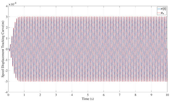
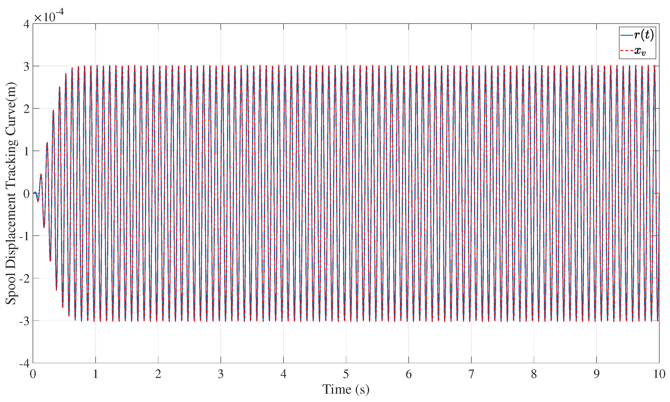
Figure 3 shows the displacement tracking response of the RDDV under the proposed ANNPTC method. The actual spool displacement $x_v$ closely follows the desired trajectory $r\left(t\right)$ during both the transient starting stage and the steady-state sinusoidal tracking stage. No obvious amplitude attenuation, output saturation, or persistent phase lag can be observed. This indicates that the proposed controller can effectively deal with the electromechanical–hydraulic coupling dynamics and achieve accurate tracking for the $10\mathrm{Hz}$ sinusoidal command.

Figure 3. Spool displacement tracking response under the sinusoidal reference input.

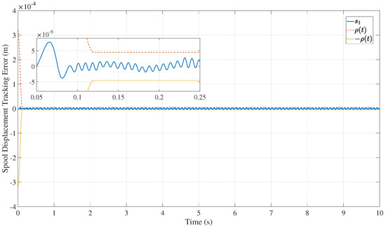
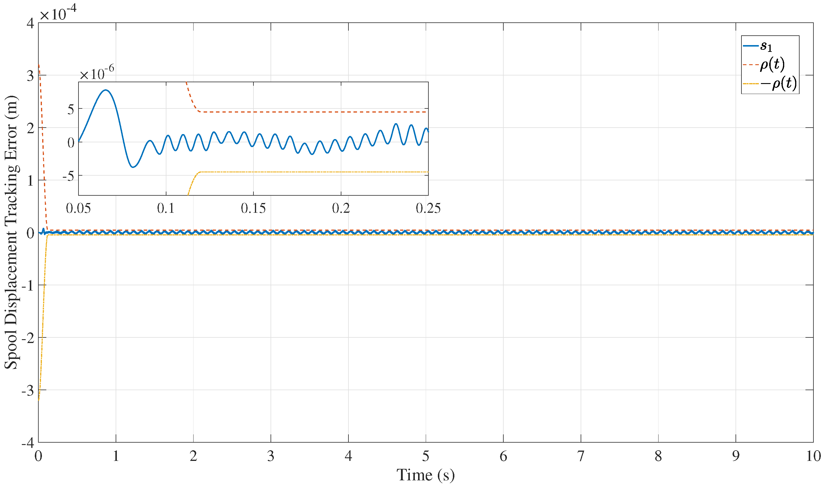
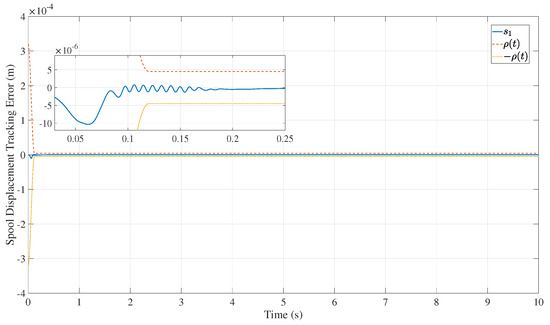
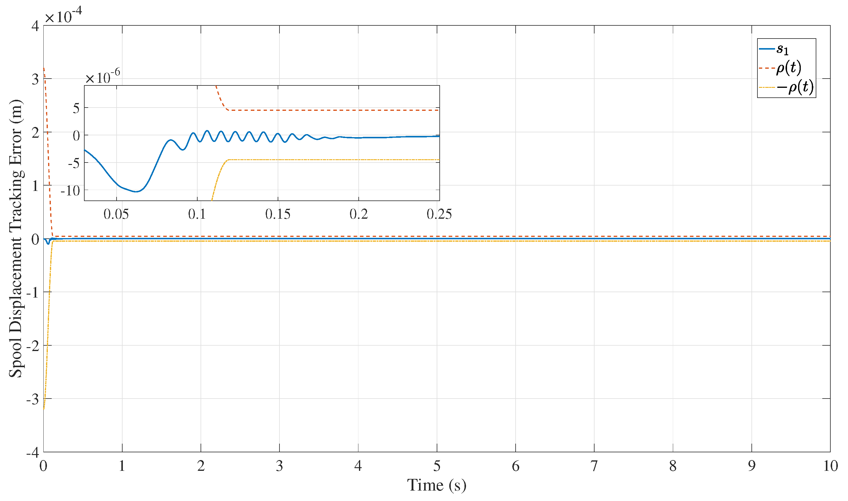
Figure 4 illustrates the tracking error $s_1$ together with the preset performance boundaries $\rho \left(t\right)$ and $-\rho \left(t\right)$. It can be seen that the tracking error remains within the prescribed boundaries throughout the simulation. At the initial stage, the boundary is relatively large, which avoids excessive transient control effort. Then, the boundary rapidly converges to the prescribed steady-state range within the preset time. The enlarged view further shows that the tracking error is constrained in a small neighborhood around zero after the transient stage. This verifies that the proposed ANNPTC can enforce the preset-time performance requirement on the spool displacement error.

Figure 4. Tracking error constrained by the preset-time performance boundary.

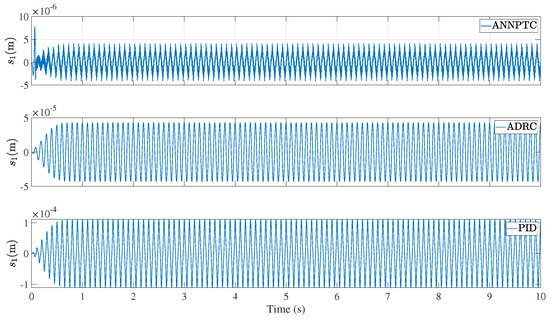
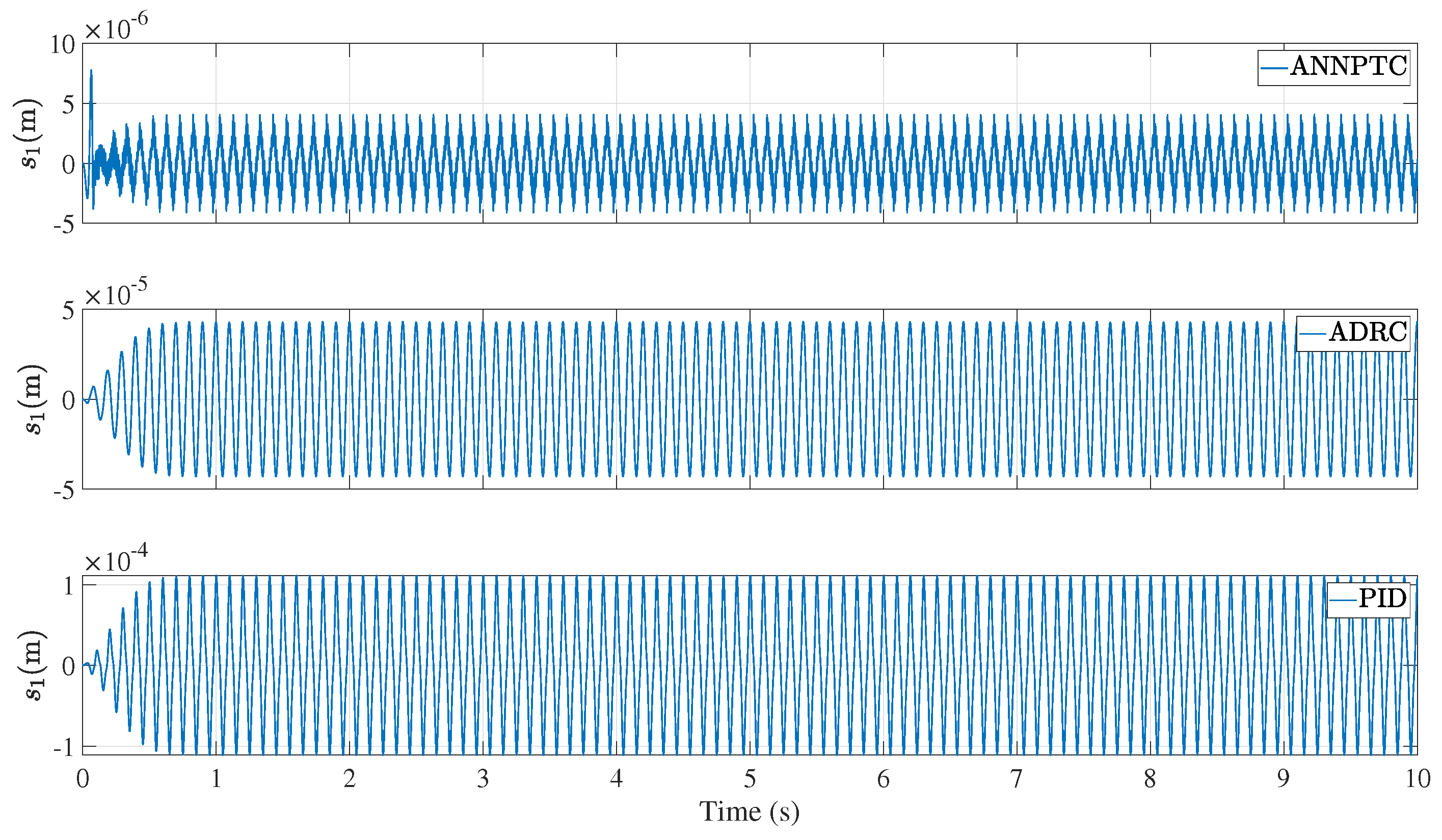
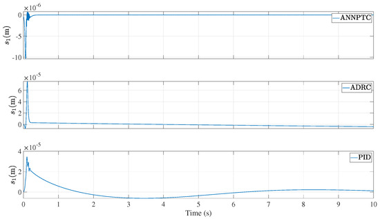
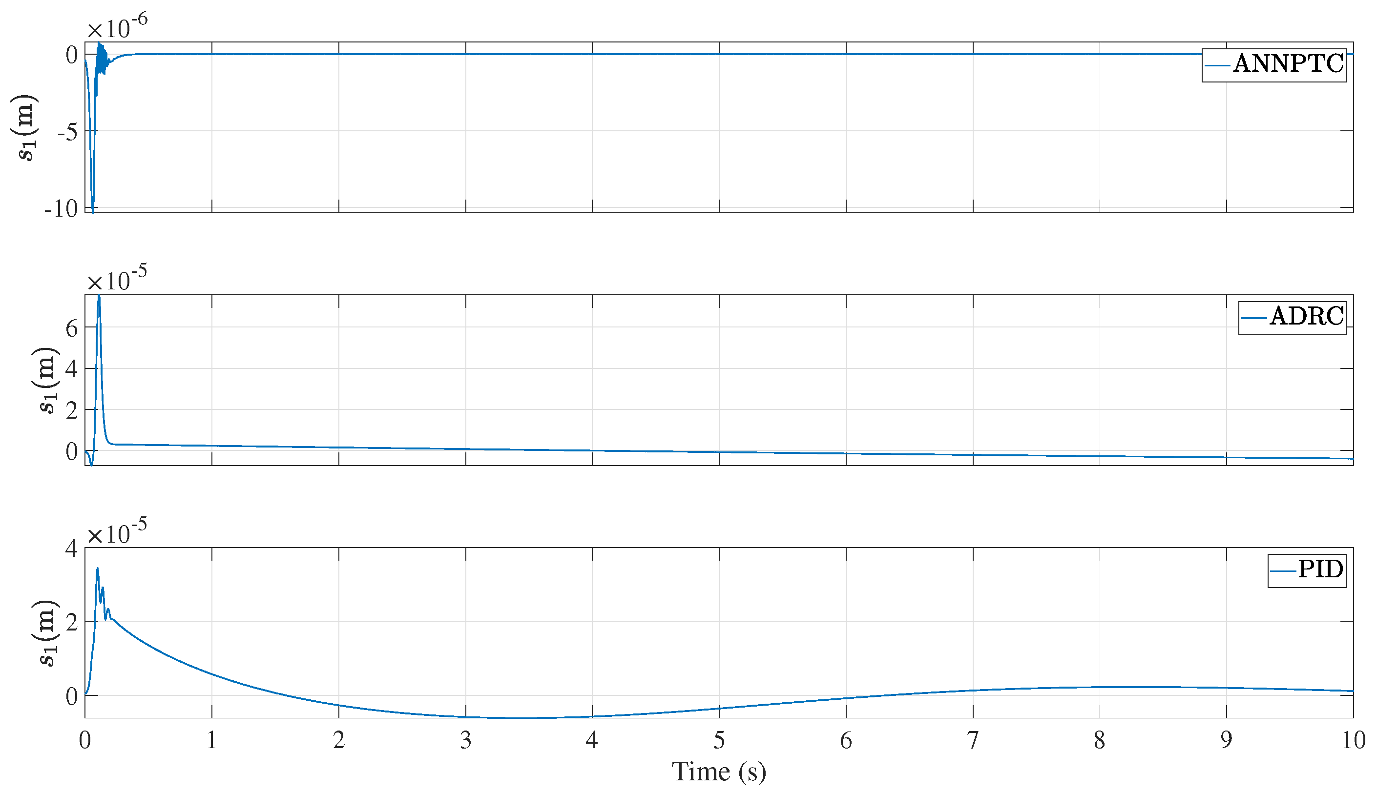
Figure 5 compares the tracking errors of ANNPTC, ADRC, and PID controllers under the same sinusoidal reference input. A detailed quantitative analysis of the tracking error curves is presented in Table 5 below. The maximum absolute tracking error of the proposed ANNPTC is $7.781\times {10}^{-6}\mathrm{m}$, which is much smaller than $4.969\times {10}^{-4}\mathrm{m}$ for ADRC and $1.111\times {10}^{-4}\mathrm{m}$ for PID. The steady-state error and RMSE of ANNPTC are also only $1.639\times {10}^{-6}\mathrm{m}$ and $1.938\times {10}^{-6}\mathrm{m}$, respectively, whereas the corresponding values are $3.469\times {10}^{-4}\mathrm{m}$ and $3.288\times {10}^{-4}\mathrm{m}$ for ADRC and $5.828\times {10}^{-5}\mathrm{m}$ and $6.772\times {10}^{-5}\mathrm{m}$ for PID. These three indicators consistently show that ANNPTC has the best overall tracking performance in Case 1. Compared with the two baseline controllers, ANNPTC achieves the smallest tracking error and shows better steady-state accuracy. This improvement is mainly attributed to the preset-time error constraint, the backstepping stabilization structure, and the adaptive RBFNN compensation for the unknown nonlinear dynamics of the RDDV.

Figure 5. Tracking error comparison among ANNPTC, ADRC, and PID controllers.

Table 5. Quantitative analysis of tracking error for Case 1.

	ANNPTC	ADRC	PID
Maximum absolute tracking error/m	$7.781\times {10}^{-6}$	$4.969\times {10}^{-4}$	$1.111\times {10}^{-4}$
Steady-state error/m (average absolute value of the last $20\%$)	$1.639\times {10}^{-6}$	$3.469\times {10}^{-4}$	$5.828\times {10}^{-5}$
RMSE/m	$1.938\times {10}^{-6}$	$3.288\times {10}^{-4}$	$6.772\times {10}^{-5}$

To sum up, the results of Case 1 demonstrate that the proposed ANNPTC method can achieve high-precision sinusoidal tracking while satisfying the prescribed-performance constraint. Compared with ADRC and PID, the proposed method provides better tracking accuracy and stronger robustness against the nonlinear and uncertain dynamics involved in the RDDV model.

4.3. Case 2: Smooth Step Reference Tracking

In the second simulation case, a step-type displacement command is used to further evaluate the cross-condition applicability of the proposed ANNPTC method. Since the ideal step signal is discontinuous and its time derivatives are not bounded, it is not directly suitable for the backstepping-based controller, where $\dot{r}\left(t\right)$ and $\ddot{r}\left(t\right)$ are required. Therefore, a smooth step command is adopted to avoid derivative singularities and excessive initial control impact. The smooth step input is designed as

$$r\left(t\right)={\displaystyle \frac{A}{2}}\left[1+tanh\left({\displaystyle \frac{t-t_0}{T_r}}\right)\right],$$

(67)

where $A=3.0\times {10}^{-4}\mathrm{m}$ is the step amplitude, $t_0$ denotes the center time of the smooth transition, and $T_r$ determines the duration and steepness of the transition. In this case, the parameters of ANNPTC, ADRC, and PID controllers are kept the same as those used in Case 1. This setting is used to examine whether the proposed ANNPTC can maintain satisfactory performance without retuning when the reference input changes from a sinusoidal trajectory to a step-type trajectory.

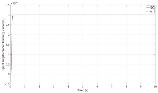
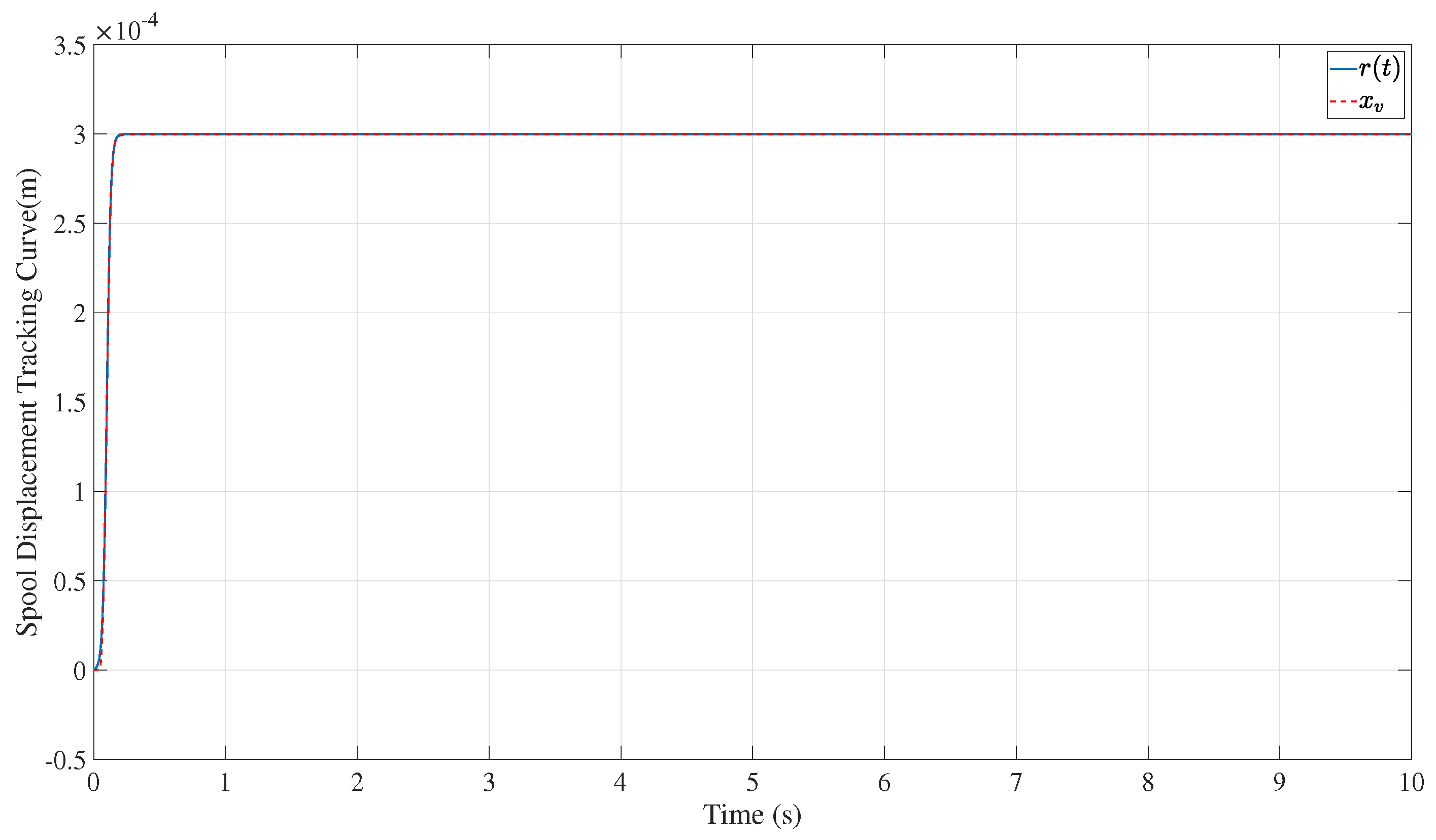
Figure 6 shows the displacement response under the smooth step reference input. The proposed ANNPTC drives the spool displacement $x_v$ to the desired value rapidly and maintains a stable, steady-state response after the transient stage. Compared with sinusoidal tracking, the step-type command imposes a stronger transient requirement on the controller. Nevertheless, the ANNPTC still achieves accurate position regulation without changing its control parameters, indicating that the proposed method has good applicability to different reference trajectories.

Figure 6. Spool displacement tracking response under the smooth step reference input.

Figure 7 presents the tracking error $s_1$ and the preset performance boundaries. The error remains within the prescribed boundary during the whole response process. At the beginning of the step transition, the performance boundary provides an allowable transient region to avoid excessive control action. After the preset time, the boundary converges to the steady-state range, and the tracking error is confined to a small neighborhood around zero. This result verifies that the preset-time constraint remains effective in the step response case.

Figure 7. Tracking error constrained by the preset-time performance boundary under the smooth step input.

Figure 8 compares the tracking errors of ANNPTC, ADRC, and PID controllers. A detailed quantitative analysis of the tracking error curves is presented in Table 6 below. Under the same controller parameters as those in Case 1, the ANNPTC error converges rapidly and remains smaller than that of the comparative controllers. The maximum absolute tracking error is only $1.035\times {10}^{-5}\mathrm{m}$, compared with $7.577\times {10}^{-5}\mathrm{m}$ for ADRC and $3.446\times {10}^{-5}\mathrm{m}$ for PID. In addition, ANNPTC gives a steady-state error of $8.547\times {10}^{-9}\mathrm{m}$ and an RMSE of $5.527\times {10}^{-7}\mathrm{m}$, both lower than the corresponding ADRC values of $3.336\times {10}^{-6}\mathrm{m}$ and $4.870\times {10}^{-6}\mathrm{m}$ and the PID values of $1.893\times {10}^{-6}\mathrm{m}$ and $5.775\times {10}^{-6}\mathrm{m}$. Therefore, ANNPTC provides the best control performance among the three controllers in Case 2. This is primarily because the ADRC and PID controllers struggle to effectively handle abrupt changes in control signals. compared to the controller proposed in this paper, while the proposed ANNPTC combines preset performance regulation, backstepping stabilization, and RBFNN-based adaptive compensation. Therefore, it can better accommodate the nonlinear and uncertain dynamics of the RDDV under different reference inputs.

Figure 8. Tracking error comparison among ANNPTC, ADRC, and PID controllers under the smooth step input.

Table 6. Quantitative analysis of tracking error for Case 2.

	ANNPTC	ADRC	PID
Maximum absolute tracking error/m	$1.035\times {10}^{-5}$	$7.577\times {10}^{-5}$	$3.446\times {10}^{-5}$
Steady-state error/m (average absolute value of the last $20\%$)	$8.547\times {10}^{-9}$	$3.336\times {10}^{-6}$	$1.893\times {10}^{-6}$
RMSE/m	$5.527\times {10}^{-7}$	$4.870\times {10}^{-6}$	$5.775\times {10}^{-6}$

Overall, the results of Case 2 show that the proposed ANNPTC method can still guarantee accurate tracking and prescribed performance under the smooth step input without controller retuning. Together with the sinusoidal tracking results in Case 1, this demonstrates the broader applicability and stronger robustness of ANNPTC compared with ADRC and PID controllers.

4.4. Case 3: Smooth Square-Wave Reference Tracking

In the third simulation case, a square-wave displacement command is introduced to further evaluate the dynamic adaptability and repeated transient tracking capability of the proposed ANNPTC method. Compared with the smooth step command in Case 2, the square-wave reference contains periodic rising and falling transitions, which impose more frequent acceleration and deceleration requirements on the RDDV spool. However, an ideal square wave is discontinuous, and its derivatives are unbounded at the switching instants, which is not suitable for the backstepping-based controller requiring the first- and second-order derivatives of the reference signal. Therefore, a smooth square-wave command is adopted in this case to preserve differentiability while retaining the main characteristics of a square-wave trajectory. The reference signal is designed as

$$r\left(t\right)={\displaystyle \frac{A}{2}}\left[1+tanh\left(\beta \left[-cos\left(2\pi f_{s}t\right)\right]\right)\right],$$

(68)

where $A=3.0\times {10}^{-4}\mathrm{m}$ is the displacement amplitude, $f_s=2\mathrm{Hz}$ is the square-wave frequency, and $\beta =10.0$ is a positive smoothing coefficient used to adjust the steepness of the rising and falling edges. A larger $\beta$ makes the reference signal closer to an ideal square wave, whereas a smaller $\beta$ produces smoother transitions and weaker derivative peaks. In this case, the parameters of ANNPTC controllers are kept the same as those used in Case 1 and Case 2. However, the parameters of the ADRC and PID controllers are self-tuned for square-wave operating conditions to ensure optimal control performance. This setting is used to examine whether the proposed ANNPTC can maintain satisfactory tracking performance under periodically switching reference commands without controller retuning.

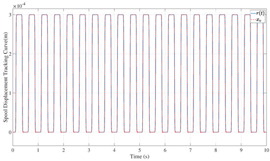
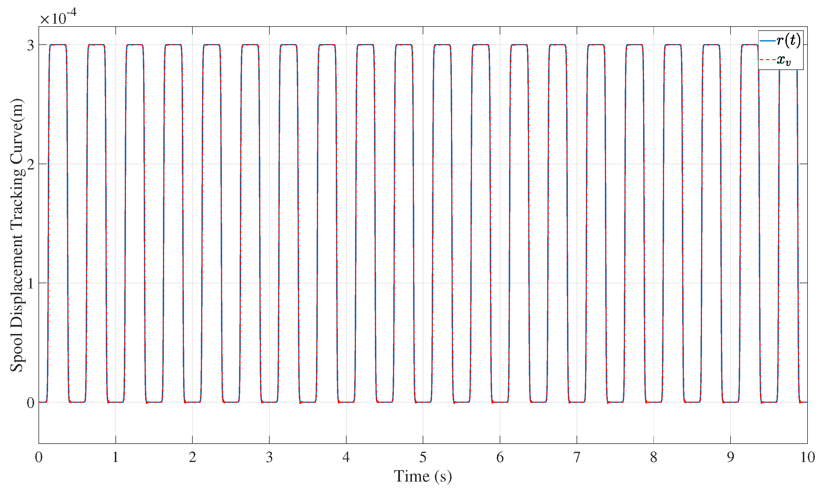
Figure 9 shows the displacement tracking response under the smooth square-wave reference input. The proposed ANNPTC enables the spool displacement $x_v$ to follow the periodic high-low displacement command accurately. Although the square-wave trajectory requires repeated rapid transitions between two displacement levels, the actual spool displacement remains closely aligned with the desired trajectory during both rising and falling stages. This indicates that the proposed method can effectively handle frequent transient changes and maintain stable tracking behavior under a periodically switching command.

Figure 9. Spool displacement tracking response under the smooth square-wave reference input.

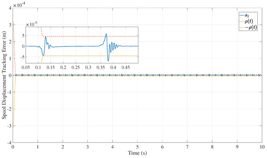
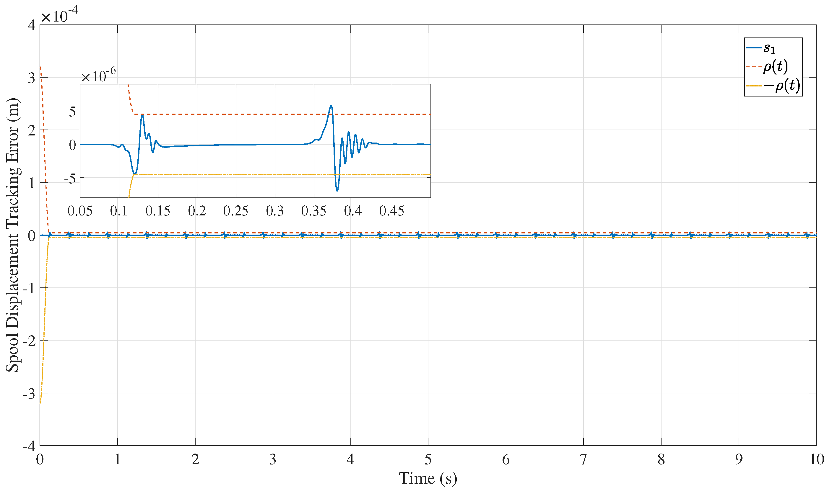
Figure 10 presents the tracking error $s_1$ and the corresponding preset performance boundaries under the smooth square-wave input. During the initial stage, the tracking error is restricted within the prescribed transient boundary. After the preset time, the boundary converges to the steady-state range, and the tracking error remains confined within a small neighborhood around zero. Although rapid changes in the reference command result in minor error fluctuations near the switching instants—exhibiting a distinct pattern where the error for a rising square wave remains within the preset-time-varying bounds while the error for a falling square wave temporarily exceeds them—the compensation calculations provided by the ANNPTC control scheme enable the error to converge rapidly to a steady state; overall, the system can be considered to satisfy the prescribed-performance constraints. This result demonstrates that the preset-time performance mechanism remains valid not only for single-transition step tracking but also for repeated-transition square-wave tracking.

Figure 10. Tracking error constrained by the preset-time performance boundary under the smooth square-wave input.

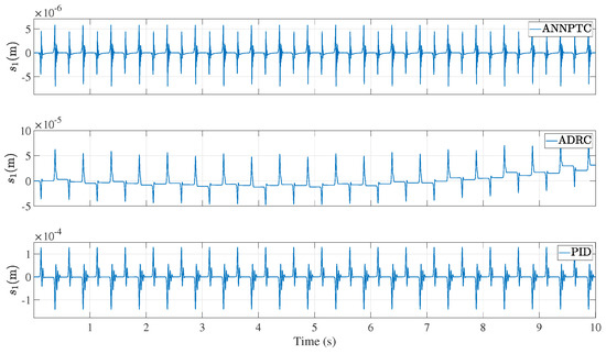
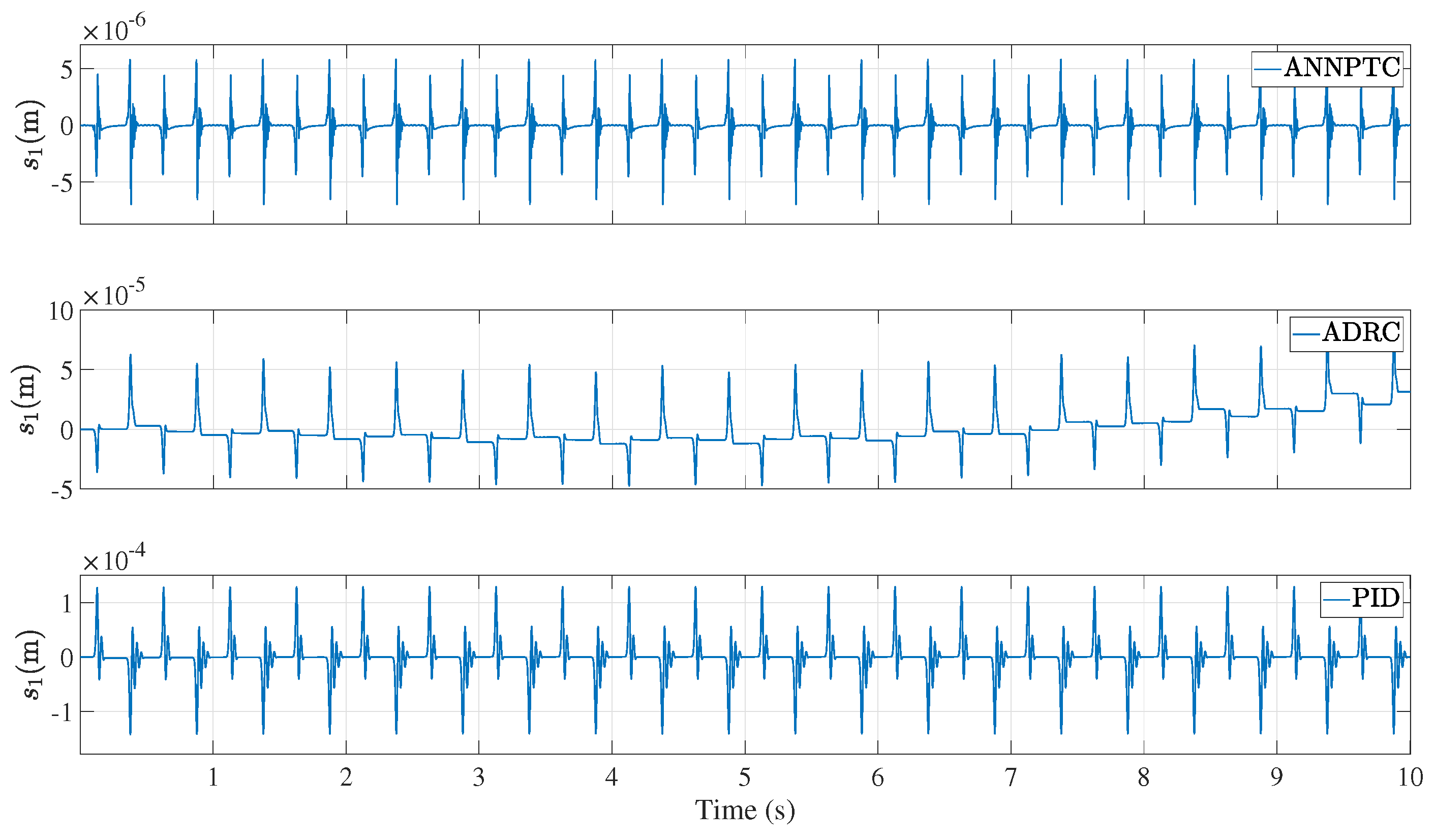
Figure 11 compares the tracking errors of ANNPTC, ADRC, and PID controllers under the smooth square-wave command. A detailed quantitative analysis of the tracking error curves is presented in Table 7 below. The proposed ANNPTC maintains a smaller tracking error during both steady intervals and switching intervals. The maximum absolute tracking error of ANNPTC is $6.963\times {10}^{-6}\mathrm{m}$, while the ADRC and PID controllers produce larger peaks of $8.050\times {10}^{-5}\mathrm{m}$ and $1.426\times {10}^{-4}\mathrm{m}$, respectively. The steady-state error and RMSE are also reduced to $4.951\times {10}^{-7}\mathrm{m}$ and $1.218\times {10}^{-6}\mathrm{m}$ for ANNPTC, compared with $1.893\times {10}^{-5}\mathrm{m}$ and $1.491\times {10}^{-5}\mathrm{m}$ for ADRC and $1.343\times {10}^{-5}\mathrm{m}$ and $3.102\times {10}^{-5}\mathrm{m}$ for PID. These results indicate that ANNPTC provides the best overall control performance in terms of transient peak suppression, steady-state accuracy, and global tracking accuracy. This is mainly because the square-wave trajectory repeatedly excites the nonlinear dynamics, uncertain disturbances, and transient response limitations of the RDDV system. Owing to the integration of preset performance regulation, backstepping stabilization, and RBFNN-based adaptive compensation, the proposed ANNPTC can better compensate for the uncertain nonlinear dynamics and suppress the transient error induced by repeated reference switching.

Figure 11. Tracking error comparison among ANNPTC, ADRC, and PID controllers under the smooth square-wave input.

Table 7. Quantitative analysis of tracking error for Case 3.

	ANNPTC	ADRC	PID
Maximum absolute tracking error/m	$6.963\times {10}^{-6}$	$8.050\times {10}^{-5}$	$1.426\times {10}^{-4}$
Steady-state error/m (average absolute value of the last $20\%$)	$4.951\times {10}^{-7}$	$1.893\times {10}^{-5}$	$1.343\times {10}^{-5}$
RMSE/m	$1.218\times {10}^{-6}$	$1.491\times {10}^{-5}$	$3.102\times {10}^{-5}$

Overall, the results of Case 3 show that the proposed ANNPTC method can still guarantee accurate tracking and prescribed performance under a smooth square-wave input without controller retuning. Together with the sinusoidal tracking result in Case 1 and the smooth step tracking result in Case 2, this further verifies the cross-condition applicability, transient robustness, and reference adaptability of the proposed ANNPTC method for RDDV displacement control.

In summary, a sensitivity analysis is further conducted to evaluate the influence of RBFNN initialization, radial node number, object parameter variations, and calculation frequency. First, different initial neural weights are tested while keeping the same controller gains. The control performance of the system under optimal weights is presented in this section. The results show that the initial weights mainly affect the early transient compensation process, whereas the final tracking accuracy remains close because the adaptive laws update the weights online and the leakage terms keep them bounded. Second, different numbers of radial basis function nodes are compared during the simulation process. When the number of nodes is too small, the approximation capability is insufficient, and the tracking error increases. When the number of nodes is moderately increased, the tracking performance becomes similar, indicating that further increasing the node number brings limited accuracy improvement but increases computational cost. Third, the unknown dynamics defined in the theoretical derivation section are modeled in the simulation as time-varying functions dependent on the control variables, thereby simulating scenarios where system parameters change. The proposed controller maintains stable tracking because these parameter variations are absorbed into the lumped unknown dynamics and compensated by the RBFNN. Finally, the influence of the calculation frequency is examined. A sufficiently high calculation frequency is required because the preset-time boundary, virtual control derivatives, and adaptive laws are updated online. If the sampling interval is too large, the discretization error increases and the tracking performance deteriorates. In this study, the selected sampling time provides a proper balance between numerical accuracy and real-time computational burden.

5. Conclusions

In this study, an adaptive neural network preset-time control method was developed for the position tracking problem of a rotary direct-drive valve with unknown nonlinear dynamics and external disturbances. A refined electromechanical–hydraulic model of the RDDV was first established by considering the motor electrical dynamics, eccentric-transmission mechanism, spool axial dynamics, nonlinear friction, hydraulic flow force, and lumped uncertainties. Based on this model, the RDDV dynamics were transformed into a control-oriented strict-feedback form, and RBF neural networks were introduced to approximate the lumped unknown dynamics.

A preset-time performance function was incorporated into the backstepping design to constrain the spool displacement tracking error within a prescribed boundary. The Lyapunov analysis shows that all closed-loop signals are uniformly ultimately bounded and that, provided the initial tracking error is inside the prescribed initial boundary, the spool displacement tracking error remains within the preset performance constraint and enters the prescribed residual set after the user-defined time $T_c$. Therefore, the theoretical result achieves prescribed-time, prescribed-performance tracking in a practical sense, rather than convergence to zero within the prescribed time in a strict sense. Simulation results under sinusoidal, smooth step, and smooth square-wave reference inputs further indicated that the proposed ANNPTC method can achieve smaller tracking errors than the benchmark ADRC and PID controllers under the considered nonlinear disturbances and parameter settings.

Although the obtained results demonstrate the potential of the proposed method for high-precision RDDV tracking control, the present study is mainly based on numerical simulation. Future work will focus on experimental validation on an RDDV test platform, robustness evaluation under broader operating conditions, and further improvement of the controller by considering input saturation, measurement noise, and practical implementation constraints.

References

- Zhou, X.; Liu, W.; Zhou, A.; An, S.; Xu, X.; Jin, J.; Zhang, X. Dynamic characterization and structural parameter optimization of rotary direct-drive electrohydraulic servo valve. AIP Adv. 2025, 15, 035038. [Google Scholar] [CrossRef] [Scilit]
- Zhang, J.; Pan, X.; Guo, J.; Bian, J.; Kang, J. Analysis of the static and dynamic characteristics of the electro-hydraulic pressure servo valve of robot. Sci. Rep. 2023, 13, 15553. [Google Scholar] [CrossRef] [Scilit] [PubMed]
- Ding, R.; Sun, G.; Zhang, J.; Peng, L.; Cheng, M.; Xu, B.; Yang, H. A review of independent metering control system for mobile machinery. Int. J. Hydromech. 2025, 8, 1–39. [Google Scholar] [CrossRef] [Scilit]
- Chen, X.; Tang, Y.; Huang, X.; Wang, W.; Guo, J.; Lin, F.; Jia, L.; Yang, H.; Zhu, Y. Automation and synchronisation on electro-hydraulic lifting system of tunnel boring machine segment assembly. Int. J. Hydromech. 2025, 8, 94–120. [Google Scholar] [CrossRef] [Scilit]
- Cao, X.; Zhao, Z.; Zhu, W.; Lian, G.; Ye, M.; Alam, M.M. Ride comfort analysis of hydro-pneumatic suspension considering variable damping matched with dynamitic load. Int. J. Hydromech. 2025, 8, 317–342. [Google Scholar] [CrossRef] [Scilit]
- Lu, L.; Xia, F.; Yin, Y.; Yuan, J.; Guo, S. Spool stuck mechanism of ball-type rotary direct drive pressure servo valve. J. ZheJiang Univ. Eng. Sci. 2019, 53, 1265–1273. [Google Scholar]
- Yuan, J.; Yan, Y.; Xia, F.; Fang, X. Stability analysis of rotary direct drive electrohydraulic pressure control servo valve. J. Tongji Univ. (Natural Sci. Ed.) 2018, 46, 235–240. [Google Scholar]
- Li, Y. Steady-state modelling and performance of a rotary direct drive digital valve. Meas. Control 2020, 53, 311–319. [Google Scholar] [CrossRef] [Scilit]
- Yang, X.; Ge, Y.; Deng, W.; Yao, J. Precision motion control for electro-hydraulic axis systems under unknown time-variant parameters and disturbances. Chin. J. Aeronaut. 2024, 37, 463–471. [Google Scholar] [CrossRef] [Scilit]
- Yang, X.; Deng, W.; Yao, J. Motion control design for an electro-hydraulic actuator under ensured performance. Chin. J. Aeronaut. 2025, 39, 103828. [Google Scholar] [CrossRef] [Scilit]
- Xiao, M.; Zeng, M.; Li, Y.; Wu, K.; Ni, Y.; Lan, N. Drive control of proportional valves based on active disturbance rejection control. Eng. Res. Express 2025, 7, 025012. [Google Scholar] [CrossRef] [Scilit]
- Niu, S.; Wang, J.; Zhao, J.; Shen, W. Neural network-based finite-time command-filtered adaptive backstepping control of electro-hydraulic servo system with a three-stage valve. ISA Trans. 2024, 144, 419–435. [Google Scholar] [CrossRef] [Scilit] [PubMed]
- Zhao, L.; Yu, J.; Wang, Q.G. Finite-time tracking control for nonlinear systems via adaptive neural output feedback and command filtered backstepping. IEEE Trans. Neural Netw. Learn. Syst. 2020, 32, 1474–1485. [Google Scholar] [CrossRef] [Scilit]
- Xing, Y.; Wang, Y. Finite-time adaptive NN backstepping dynamic surface control for input-delay fractional-order nonlinear systems. IEEE Access 2023, 11, 5206–5214. [Google Scholar] [CrossRef] [Scilit]
- Chen, M.; Li, Y.; Wang, H.; Peng, K.; Wu, L. Adaptive fixed-time tracking control for nonlinear systems based on finite-time command-filtered backstepping. IEEE Trans. Fuzzy Syst. 2022, 31, 1604–1613. [Google Scholar]
- Wang, C.; Wang, J.; Guo, Q.; Ren, X.; Cao, Y.; Jiang, D. Fixed-time adaptive neural control of electro-hydraulic system with model uncertainties: Theory and experiments. Control Eng. Pract. 2024, 147, 105931. [Google Scholar] [CrossRef] [Scilit]
- Lu, K.; Liu, Z.; Wang, Y.; Chen, C.P. Fixed-time adaptive fuzzy control for uncertain nonlinear systems. IEEE Trans. Fuzzy Syst. 2020, 29, 3769–3781. [Google Scholar]
- Dong, Z.; Bai, D.; Zhang, P.; Yao, J. Prescribed performance adaptive neural network tracking control of electro-hydraulic servo system with input delay. Appl. Math. Model. 2025, 152, 116591. [Google Scholar] [CrossRef] [Scilit]
- Yang, X.; Ge, Y.; Zhu, W.; Deng, W.; Zhao, X.; Yao, J. Adaptive motion control for electro-hydraulic servo systems with appointed-time performance. IEEE/ASME Trans. Mechatron. 2025, 30, 7009–7018. [Google Scholar] [CrossRef] [Scilit]
- Wan, Y.; Yue, W.; Gao, X.; Chen, Q.; Xu, R. Adaptive finite-time prescribed performance tracking control for hydraulic servo systems with friction compensation. Neurocomputing 2024, 564, 126967. [Google Scholar] [CrossRef] [Scilit]
- Liu, H.; Wang, R.; Sun, F.; Xing, X. Adaptive self-structuring neural network control for full-state constrained hydraulic systems with disturbance compensation. Appl. Math. Model. 2024, 129, 1–24. [Google Scholar] [CrossRef] [Scilit]
- Fang, Y.; Zhang, J.; Li, Y. Neural networks adaptive predefined-time control for pure-feedback nonlinear systems: A case study on robotic exoskeleton systems. Sci. Rep. 2025, 15, 6041. [Google Scholar] [PubMed]
- Yang, X.; Deng, W.; Yao, J. Neural adaptive dynamic surface asymptotic tracking control of hydraulic manipulators with guaranteed transient performance. IEEE Trans. Neural Netw. Learn. Syst. 2022, 34, 7339–7349. [Google Scholar] [CrossRef] [Scilit]
- Jiang, W.; Wang, H.; Zhao, X. A novel adaptive neural predefined time control for a class of nonlinear systems. Asian J. Control 2024, 26, 2441–2450. [Google Scholar] [CrossRef] [Scilit]
- Hua, C.; Ning, P.; Li, K. Adaptive prescribed-time control for a class of uncertain nonlinear systems. IEEE Trans. Autom. Control 2021, 67, 6159–6166. [Google Scholar] [CrossRef] [Scilit]
- Phan, V.D.; Truong, H.V.A.; Le, V.C.; Ho, S.P.; Ahn, K.K. Adaptive neural observer-based output feedback anti-actuator fault control of a nonlinear electro-hydraulic system with full state constraints. Sci. Rep. 2025, 15, 3044. [Google Scholar] [CrossRef] [Scilit] [PubMed]
- Zhang, J.; Wei, X.; Li, N.; Pan, X.; Sun, Y. Durability analysis of rotary direct drive electro-hydraulic pressure servo valve based on failure physics principle. PLoS ONE 2025, 20, e0316711. [Google Scholar] [CrossRef] [Scilit] [PubMed]
- Márton, L.; Fodor, S.; Sepehri, N. A practical method for friction identification in hydraulic actuators. Mechatronics 2011, 21, 350–356. [Google Scholar] [CrossRef] [Scilit]
- Tran, X.B.; Khaing, W.H.; Endo, H.; Yanada, H. Effect of friction model on simulation of hydraulic actuator. Proc. Inst. Mech. Eng. Part I J. Syst. Control Eng. 2014, 228, 690–698. [Google Scholar] [CrossRef] [Scilit]
- Yao, J.; Deng, W.; Jiao, Z. Adaptive control of hydraulic actuators with LuGre model-based friction compensation. IEEE Trans. Ind. Electron. 2015, 62, 6469–6477. [Google Scholar] [CrossRef] [Scilit]
Disclaimer/Publisher’s Note: The statements, opinions and data contained in all publications are solely those of the individual author(s) and contributor(s) and not of MDPI and/or the editor(s). MDPI and/or the editor(s) disclaim responsibility for any injury to people or property resulting from any ideas, methods, instructions or products referred to in the content. |
© 2026 by the authors. Licensee MDPI, Basel, Switzerland. This article is an open access article distributed under the terms and conditions of the Creative Commons Attribution (CC BY) license.