


Abstract
Real-time industrial anomaly detection is increasingly shifting from cloud-based diagnosis to edge intelligence deployed close to machines. However, practical industrial scenarios are constrained by scarce fault samples, unknown anomaly types, cross-machine distribution shifts, strict false alarm requirements, data privacy restrictions, and limited edge device resources. To address these challenges, this paper proposes EPC-TinyAD, an energy- and privacy-aware compressed TinyML framework for reliable industrial anomaly detection on resource-constrained edge devices. EPC-TinyAD follows a normal-only learning paradigm and employs a tiny depthwise-separable CNN autoencoder as the deployable student model, guided by a wider teacher autoencoder during training. Instead of relying solely on reconstruction error, the proposed anomaly score integrates spectrogram reconstruction deviation, compact normal-center distance, and teacher–student distillation discrepancy. Masked spectrogram modeling is introduced to enhance few-shot normal representation learning, while domain-adversarial invariant embedding improves cross-machine generalization. To support reliable deployment, split and adaptive conformal thresholding calibrate anomaly decisions under target false alarm rates. Furthermore, federated training with clipped and noisy updates reduces raw industrial data exposure, and energy-aware compression integrates pruning, INT8 size estimation, model export, latency benchmarking, and Pareto analysis. Experiments on industrial anomaly detection data demonstrate that EPC-TinyAD achieves 96.5% accuracy, 95.4% recall, 96.1% F1 score, 0.964 AUROC, and 0.952 AUPRC over five random seeds. These results indicate that EPC-TinyAD provides a reliable, lightweight, privacy-aware, and deployment-oriented framework for industrial edge anomaly detection, while future work will further validate its runtime memory, latency, and power consumption on physical Raspberry Pi-, Jetson-, or MCU-class edge devices.
1. Introduction
With the rapid development of the industrial Internet of Things, intelligent manufacturing, and edge computing, real-time condition monitoring for critical equipment such as rotating machinery, pumps, valves, fans, slides, and bearings is gradually shifting from traditional cloud-based analysis to edge intelligence deployed close to data sources [1]. Industrial equipment continuously generates acoustic, vibration, current, or multimodal sensing signals during operation [2], where anomalous patterns often correspond to early-stage wear, structural loosening, lubrication degradation, impact damage, or potential shutdown risks [3]. Therefore, constructing an intelligent diagnostic system capable of real-time identification of unknown anomalies on low-power edge devices is of great significance for reducing unplanned downtime, improving equipment reliability, and ensuring industrial production safety. However, industrial anomaly detection is substantially different from general visual or speech recognition tasks. Real fault samples are usually scarce, non-exhaustive, and difficult to collect, so only normal operating data are often available during training [4]. In addition, machine type, device ID, load condition, and acquisition environment may cause significant cross-domain distribution shifts [5]. Industrial sites are also highly sensitive to false alarms because frequent false positives can lead to unnecessary maintenance, production line interruptions, and increased operating costs [6]. Therefore, anomaly detection systems for real-world edge deployment should not only pursue high offline AUROC. They must also support unknown anomaly recognition, cross-device generalization, controllable false alarm rates, privacy preservation, model lightweighting, and low-energy inference [7].
Existing industrial anomaly detection methods mainly include autoencoder-based reconstruction error approaches [8], one-class classification-based compact representation methods [9], deep embedding distance-based anomaly scoring schemes [10], and recently emerged knowledge distillation and self-supervised representation learning methods [11]. These methods have achieved certain progress on offline datasets but still show obvious shortcomings in practical applications for resource-constrained edge devices. First, many methods assume that the training and test sets follow similar distributions and struggle to handle domain shifts across different machines, sections, source/target domains, or new equipment scenarios [12]. Second, single reconstruction error often suffers from the defect that “anomalies can also be well reconstructed”, resulting in insufficient discrimination for unknown anomalies [13]; purely discriminative methods rely on anomaly labels and are unsuitable for industrial normal-only scenarios [14]. Third, existing lightweighting studies often treat compression as a postprocessing step and only report reductions in model size or parameter count, lacking a systematic Pareto analysis among accuracy, latency, energy consumption, memory usage, and deployment formats [15]. Fourth, industrial data usually involve equipment conditions, production line status, and enterprise production privacy; direct centralized uploading of raw data for training entails data leakage risks [16]. Finally, many studies still use fixed percentile or empirical thresholds for anomaly decision-making, lacking a statistical calibration mechanism for target false positive rates and making it difficult to meet industrial requirements for low false alarms, interpretable thresholds, and stable alarm strategies [17].
To address the above issues, this paper proposes an Energy- and Privacy-aware Compressed TinyML [18] Anomaly Detection Framework for resource-constrained industrial edge deployment, named EPC-TinyAD. Taking industrial acoustic/vibration signals as input, the framework converts raw sensing signals into log-Mel time–frequency representations and adopts a Tiny depthwise-separable CNN autoencoder as the edge-deployed student model [19], with a wider teacher autoencoder network for performance guidance during training [20]. Different from traditional methods that rely only on reconstruction error, EPC-TinyAD formulates anomaly scores as a fusion of reconstruction error, distance to the normal embedding center, and teacher–student distillation discrepancy [21]. Specifically, it characterizes the deviation of samples at three levels—signal structure, normal manifold compactness, and knowledge consistency—via Srec, Scenter, and Skd. The training objective consists of reconstruction loss, one-class center constraint loss, and distillation loss, enabling the student model to inherit the teacher model’s expressive power for normal machine sound structures as much as possible while maintaining a TinyML-friendly structure [22] and forming a compact normal embedding space suitable for unknown anomaly detection. This design allows the model to perform anomaly modeling using only normal samples and alleviate degraded representation ability after model compression, providing a more stable detection foundation for real-time edge deployment [23].
Furthermore, to improve generalization under few-shot and cross-machine scenarios, this study introduces masked spectrogram modeling, self-supervised pretraining, and domain-adversarial invariant embedding learning into EPC-TinyAD [24]. In the self-supervised stage, the model learns local textures, harmonic structures, and time–frequency continuity of normal machine operating signals by randomly masking spectrogram patches and reconstructing the original log-Mel spectrograms, thereby reducing dependence on numerous labeled anomaly samples [25]. In the domain generalization stage, this paper treats machine type, device ID, section, source/target condition, or production line origin as different domains. An adversarial learning objective is constructed via a gradient reversal layer and domain discriminator, enabling the backbone encoder to retain discriminative information for anomaly detection while suppressing machine-domain-specific features and yielding more stable domain-invariant embeddings. In addition, SpecAugment, noise perturbation, and consistency regularization are introduced into normal sample training to enhance robustness against industrial background noise, acquisition disturbances, and slight condition variations. This strategy mitigates few-shot learning and cross-machine generalization challenges in industrial anomaly detection from three perspectives: structural prior learning, normal manifold compression, and cross-domain invariant representation [26].
The innovations of this study are mainly reflected in the following six aspects: First, an EPC-TinyAD framework for industrial edge deployment is proposed, which unifies normal-only unknown anomaly detection, TinyML autoencoders, teacher–student distillation, and one-class compact embedding into a single anomaly scoring mechanism, overcoming the instability of single reconstruction error and insufficient representation ability of lightweight models. Second, a masked spectrogram self-supervised pretraining strategy is designed, enabling the model to learn the time–frequency structure of normal machine sound or vibration signals in industrial scenarios lacking anomaly samples, improving representation quality under few-shot conditions. Third, domain-adversarial invariant embedding learning is introduced to improve generalization across different machine types, device IDs, operating conditions, and source/target domains via gradient reversal and domain discriminative adversarial training. Fourth, a conformal risk-controlled thresholding mechanism for industrial alarm reliability is proposed, which automatically determines anomaly thresholds under a target false positive rate α using a normal calibration set and adapts to slow distribution drift during deployment via a sliding adaptive strategy. Fifth, the federated component is reformulated as a two-mode privacy design. In the privacy-aware FedAvg mode, raw industrial signals remain on local clients and only model updates are transmitted, reducing raw data centralization but providing no formal differential privacy guarantee. In the DP-accounted FedAvg mode, client updates are clipped, a Gaussian perturbation is injected, and the cumulative client-level privacy loss is estimated by Rényi differential privacy accounting under explicitly stated assumptions. The resulting ε values quantify the privacy–utility trade-off; because the ε values obtained under the typical settings in this study remain relatively large, DP-FedAvg is interpreted as a privacy-accounted mechanism with weak practical DP protection rather than a strong-DP deployment solution. Sixth, a deployment-oriented compression and analytical energy-assessment pipeline is established, integrating global L1 pruning, INT8 deployment size estimation, TorchScript/ONNX export, software model-forward latency benchmarking, operation counting, operation-model-based analytical inference energy estimation, multi-pruning-ratio Pareto search, and bootstrap confidence interval analysis. This pipeline systematically evaluates detection performance, model size, parameter sparsity, software latency, counted computational complexity, and model-level analytical energy. However, the reported Eop values are not physical board-level voltage–current measurements and are not equivalent to real-world power consumption on Raspberry Pi-, Jetson-, or MCU-class devices. Accordingly, the energy-related conclusions of this paper are restricted to model-level analytical energy reduction under a unified counting protocol, whereas direct hardware power measurement is left as mandatory future validation.
2. Related Works
2.1. Industrial Machine Anomalous Sound Detection and Normal-Only Learning
Early research on industrial anomaly detection mainly focused on anomalous sound detection for machine condition monitoring. The MIMII dataset provides a key benchmark for this field, which contains normal and anomalous sounds of industrial machines, including valves, pumps, fans, and slide rails. Real factory background noise is mixed in to simulate actual production environments, so it has been widely used in unsupervised and semisupervised machine anomaly detection studies. DCASE 2020 Task 2 further formalized this task as an unsupervised anomalous sound detection problem, namely, “training with only normal samples and identifying unknown anomalies during the testing phase”, which better conforms to the real industrial conditions of scarce anomaly samples, open fault modes, and difficulty in exhaustive collection [27].
These benchmark studies provide a realistic problem definition and reproducible evaluation protocols for normal-only industrial anomalous sound detection. Nevertheless, their evaluation emphasis has traditionally been skewed toward threshold-independent detection metrics, especially AUROC and pAUC, whereas deployment-critical dimensions such as model footprint, inference latency, calibrated false alarm control, privacy exposure, and energy-aware compression are often treated as secondary considerations. Consequently, this line of work establishes what should be detected under normal-only learning but leaves open how such detectors can be made reliable, privacy-conscious, and resource-efficient for edge deployment.
2.2. Autoencoders, Deep SVDD, and One-Class Anomaly Detection Methods
Autoencoders are the most common basic models in unsupervised anomaly detection. Their core assumption is that the model is trained only on normal samples, resulting in a larger reconstruction error for anomalous samples. With a simple structure and stable implementation, this idea is well suited for normal-only scenarios such as MIMII/DCASE and is convenient for edge deployment. In addition to reconstruction-based methods, one-class deep learning methods such as Deep SVDD enhance the discriminability of deep anomaly detection by mapping normal samples into a compact feature space, clustering normal samples around a center, and then judging anomalies based on the distance from test samples to the center [28].
Reconstruction-based and one-class criteria provide complementary views of normality. Reconstruction error measures whether an input signal can be projected back onto the learned normal spectrogram manifold, whereas compact embedding distance evaluates whether the latent representation remains inside the normal operating region. However, conventional autoencoders may reconstruct certain abnormal samples with unexpectedly small errors, and one-class embedding methods usually do not explicitly preserve signal-level reconstruction fidelity or account for deployment overhead. A robust edge-oriented anomaly detector therefore needs to jointly consider input space fidelity, latent space compactness, and resource constraints without relying on labeled anomaly samples.
2.3. Spectral–Temporal Feature Fusion and Self-Supervised Spectrogram Modeling
In recent years, anomalous sound detection research has gradually shifted from simple log-Mel + AE to stronger spectral–temporal feature modeling. For example, STgram-MFN leverages spectral–temporal information fusion to jointly encode temporal and frequency-domain information, which is then fed into a MobileFaceNet architecture to learn fine-grained representations of normal machine sounds. This method improved AUC, pAUC, and stability on DCASE 2020 Task 2. The first-shot ASD tasks of DCASE 2024 and 2025 further emphasize rapid adaptation to new machine types, avoidance of machine-specific hyperparameter tuning, and domain generalization under conditions where the development set and evaluation set involve completely different machine types [29].
Spectral–temporal fusion and self-supervised spectrogram modeling improve the representational capacity of anomalous sound detectors by exploiting local harmonic structures, temporal continuity, and frequency-domain regularities. However, stronger representation learning is often achieved through larger acoustic backbones, pretrained models, or complex fusion modules, which may be difficult to deploy on Raspberry Pi-, Jetson-, ESP32-, or MCU-class platforms. The unresolved issue is therefore not only how to learn richer time–frequency representations but how to retain such structural knowledge under few-shot normal data while maintaining a small computational and memory footprint.
2.4. Cross-Machine Generalization, Domain Generalization, and Domain-Adversarial Learning
Cross-machine generalization has become a core challenge in industrial anomalous sound detection. DCASE 2024 Task 2 formulates the task as first-shot unsupervised ASD and requires the system to be rapidly deployed to unseen machine types under a domain generalization setting, where only one section is provided per machine type and completely different machine types are used in the development and evaluation sets. DCASE 2025 Task 2 continues this direction, emphasizing fast anomaly detection deployment for unseen machine types and avoiding machine-specific hyperparameter tuning [30].
Existing domain generalization methods commonly improve cross-domain robustness through data augmentation, pretrained acoustic models, metric learning, prototype learning, or distance-based scoring. These strategies have clarified the importance of machine-independent representations, but many of them still depend on relatively heavy feature extractors or lack explicit constraints for suppressing domain-specific nuisance information in the embedding space. The central challenge is therefore to learn normal representations that remain compact for anomaly detection, invariant across machine type, section, device ID, or source/target condition, and lightweight enough for edge-side inference.
2.5. TinyML, Lightweight Networks, and Model Compression and Deployment
TinyML and Edge AI research focus on deploying machine learning models on microcontrollers, embedded boards, and low-power edge devices. Recent surveys on TinyML/TinyDL commonly note that quantization, pruning, neural architecture search, hardware acceleration, and deployment toolchains are key enablers for on-device deep learning in practical applications. Mobile networks such as MobileNetV2 achieve a good balance between accuracy and computational cost through depthwise convolution, inverted residual, and linear bottleneck designs, providing a classic structural foundation for lightweight CNN deployment on edge devices [31].
However, much TinyML research remains centered on general image classification, keyword spotting, or object detection, whereas industrial anomaly detection imposes a different deployment objective. In this setting, lightweightness cannot be judged only by parameter count or model size; it must be evaluated jointly with anomaly detection performance, calibrated false alarm behavior, software latency, deployable model format, and model-level energy tendency. Compression should therefore be treated as part of the detection system design rather than as a postprocessing step. This perspective requires Pareto-style comparison among accuracy, memory, latency, and analytical energy under a unified deployment protocol while clearly distinguishing analytical model-level energy estimates from physical board-level power measurements.
It should be noted that lightweight comparison must be distinguished from accuracy-oriented comparison. STgram-MFN is a strong spectral–temporal representation model designed primarily for high detection accuracy in anomalous sound detection, rather than a TinyML model optimized for microcontroller- or low-power edge-board deployment. Therefore, using STgram-MFN alone to demonstrate the lightweight advantage of EPC-TinyAD would not constitute a fully fair lightweight comparison. In this study, STgram-MFN is retained only as a high-capacity, accuracy-oriented reference, while the lightweight comparison is further strengthened by introducing edge-oriented baselines, including a MobileNetV2-based spectrogram autoencoder, a squeezed convolutional variational autoencoder, a Cortex-M-class TinyML autoencoder, and a directly trained compressed TinyAE that uses the same pruning and INT8 deployment estimation pipeline as EPC-TinyAD but does not employ teacher–student distillation. This design separates two questions: whether EPC-TinyAD remains competitive against strong accuracy-oriented ASD models, and whether teacher-guided compressed TinyML learning brings measurable gains over directly trained lightweight autoencoders under the same deployment constraints.
2.6. Teacher–Student Distillation and Accuracy Recovery
Knowledge distillation was originally proposed to transfer knowledge from large models or model ensembles into smaller student models, thereby reducing inference overhead and improving deployment feasibility. For TinyML-based industrial anomaly detection, distillation is particularly critical because directly reducing model width, depth, or parameter count typically leads to degraded representation ability, which, in turn, weakens the detection of weak and subtle anomaly patterns. Recent studies on model compression have continuously used distillation, quantization, and pruning as core technical combinations for low-power deployment [32].
Most existing distillation methods are designed for supervised classification, where the student model learns class probabilities, logits, or intermediate features from a high-capacity teacher. Normal-only industrial anomaly detection is different because explicit anomaly classes are unavailable during training, and the target knowledge is not a category boundary but the structure of normal operation. In this scenario, useful distillation should preserve normal pattern reconstruction behavior, embedding consistency, and uncertainty induced by compression. This shifts the role of distillation from classification model compression to recovery of normality modeling capacity in a compact anomaly detector.
2.7. Privacy-Aware Federated Learning and Differential Privacy Accounting for Industrial Edge
Differential privacy provides a formal privacy notion by bounding the influence of an individual participant on the released training output. In federated industrial anomaly detection, this notion is relevant because factories, production lines, or machine groups may correspond to privacy-sensitive clients. However, federated learning alone does not imply differential privacy, and update clipping plus Gaussian perturbation is insufficient to justify a rigorous DP claim unless the accumulated privacy loss over client sampling and communication rounds is explicitly tracked by a privacy accountant. Therefore, it is necessary to distinguish privacy-aware federated learning, which reduces raw data exposure by keeping local sensor data on clients, from DP-accounted federated learning, which reports an approximate client-level ε-DP budget under specified assumptions [33].
To align EPC-TinyAD with formal DP terminology, this paper introduces a privacy-accounted analysis for the Gaussian-noisy FedAvg variant. In this variant, each selected client clips its model update to an L2-norm bound C, Gaussian noise with multiplier σ is injected into the aggregated update, and the cumulative privacy loss is estimated by Rényi differential privacy accounting. The resulting ε values are reported as client-level privacy budgets after T communication rounds under a fixed client sampling rate q, a failure probability δ, and a trusted aggregator or secure aggregation assumption. This design makes the privacy–utility trade-off explicit, but the reported DP protection should be interpreted according to the magnitude of ε; large ε values indicate weak practical privacy protection even if they are formally accounted.
Existing federated anomaly detection studies are still dominated by network intrusion, traffic anomaly, medical sensing, or general time-series monitoring, with comparatively limited attention to industrial machine sound detection under TinyML and energy-constrained deployment requirements. More importantly, privacy-aware federated learning and formally privacy-accounted federated learning are often not clearly separated, which can lead to overstatement of privacy guarantees. A rigorous industrial edge framework should therefore specify whether federation merely reduces raw data centralization or additionally provides an accounted DP budget and should report the accompanying utility, communication, and deployment costs.
Taken together, prior work has advanced normal-only anomaly detection, compact one-class representation, spectral–temporal modeling, domain generalization, TinyML compression, teacher–student distillation, conformal alarm calibration, and privacy-aware federated learning as important but mostly separate research directions. The remaining gap is not the absence of any single technique but the lack of an integrated deployment-calibrated framework that simultaneously addresses six coupled requirements: normal-only recognition of unknown anomalies, few-shot spectrogram representation learning, cross-machine invariant embedding, statistically calibrated false alarm control, privacy-aware or DP-accounted multi-site training, and compression-aware edge deployment evaluation. EPC-TinyAD is motivated by this gap and is designed to connect these elements within a unified industrial edge anomaly detection framework while explicitly separating methodological claims from empirical deployment evidence and from formal privacy assumption boundaries.
3. Methodology
3.1. Problem Formulation and Framework Overview
This study addresses normal-only industrial anomaly detection under edge deployment constraints. Let () denote the log-Mel spectrogram extracted from the (i)-th industrial acoustic or vibration signal, where (F) and (T) represent the frequency and temporal dimensions, respectively. During training, only samples collected under normal operating conditions are used, whereas both normal and unseen anomalous samples are included during testing. The objective is to learn a compact normality representation from normal samples and to assign higher anomaly scores to samples that deviate from the learned normal manifold.
To avoid mixing algorithmic formulation with experimental protocol and empirical evidence, this section is restricted to the methodological core of EPC-TinyAD. Specifically, Section 3 defines the TinyML encoder–decoder architecture, the architecture-aware compression design, the normality-preserving training objective, masked spectrogram modeling, domain-adversarial invariant learning, multi-component anomaly scoring, conformal thresholding, and the federated optimization mechanism. Dataset construction, hyperparameter values, privacy accountant configuration, threat model evaluation protocol, latency benchmarking, communication cost calculation, privacy budget results, and deployment-oriented numerical comparisons are reported separately in Section 4 and Section 5. This separation clarifies the boundary between method design, experimental settings, and empirical results.For example, Figure 1 is an overall architecture and training diagram of the full deployment pipeline in this study.
Figure 1.
Overall architecture and training of EPC-TinyAD to deployment pipeline.
To avoid mixing algorithmic formulation with experimental protocol and empirical evidence, this section is restricted to the core methodological components of EPC-TinyAD. Specifically, Section 3 defines the TinyML encoder–decoder architecture, architecture-aware compression operators, the normality-preserving training objective, masked spectrogram modeling, domain-adversarial invariant embedding learning, multi-component anomaly scoring, and conformal decision calibration. The federated learning component is not treated as another loss-level technique parallel to reconstruction, distillation, or conformal calibration. Instead, it is regarded as an optional system-level training paradigm for multi-site industrial collaboration, and its protocol, privacy accounting assumptions, communication cost, and threat model are reported separately in Section 4.6. Similarly, deployment benchmarking, latency measurement, operation-level analytical energy estimation, privacy budget results, and empirical performance comparisons are reported in Section 4 and Section 5. This hierarchical separation clarifies the distinction among model design, training paradigm, deployment protocol, and empirical evidence.
3.2. TinyML Encoder–Decoder Architecture
Let denote the log-Mel spectrogram of the (i)-th industrial signal. EPC-TinyAD uses a depthwise-separable convolutional autoencoder as the deployable student model. The student network is denoted as:
where , , and are the encoder, decoder, and projection head, respectively.
For the (l)-th encoder block, the hidden representation is computed as:
where (), denotes depthwise convolution, denotes pointwise convolution, denotes batch normalization, and is the nonlinear activation function. The encoded tensor is .
The compact embedding is obtained by global average pooling and linear projection:
where and is a small numerical constant. The reconstructed spectrogram is A teacher autoencoder uses the same input representation and output form but a larger width multiplier. The teacher model is used only during training and is not deployed during inference.
3.3. Compression Operators and Analytical Energy Assessment for TinyML Deployment
Let denote the trainable weights of the student model. For a target pruning ratio (p), global magnitude pruning is applied to convolutional and linear weights. The pruning threshold is defined as the (p)-quantile of the absolute values of all prunable weights:
The binary pruning mask of layer (l) is:
and the pruned weight tensor is
After pruning, the student model is fine-tuned using the same training objective defined in Section 3.4. For low-bit deployment analysis, a (b)-bit affine quantization operator is defined as:
where and are the scale and zero point, respectively. The corresponding dequantized value is:
The estimated parameter storage of a compressed model is:
where denotes the number of retained parameters in layer (l). Model export to TorchScript or ONNX is treated as a deterministic transformation of the trained student model:
Candidate selection, latency measurement, energy estimation, and Pareto-front analysis are reported in the experimental protocol and the Results Section rather than in this methodological subsection.
In addition to parameter storage and exportability, EPC-TinyAD uses an operation-model-based analytical inference energy estimate to compare compressed deployment candidates under a unified counting protocol. For a deployment candidate with pruning ratio (p) and deployment precision (b), the analytical energy per inference is defined as:
where , and denote the counted numbers of multiplications, accumulations, on-chip memory access events, and off-chip memory access events for one model-forward pass, respectively. The coefficients are precision-dependent unit energy constants used only for model-level analytical comparison. The reported values therefore quantify the energy tendency implied by counted arithmetic and memory access events under the same exported model graph and counting assumptions.
This analytical estimate should not be interpreted as measured power consumption or measured energy per inference on a physical edge board. In particular, it does not model platform-specific idle power, voltage–frequency scaling, cache behavior, memory bank conflicts, direct memory access, operating system scheduling, quantized kernel implementation, sparse operator support, accelerator utilization, or audio acquisition and preprocessing overhead. It also does not capture the substantial instruction set and microarchitectural differences among hardware platforms. For example, an INT8 depthwise convolution may be executed through highly optimized CMSIS-NN kernels on an ARM Cortex-M device, through different DSP or vector extensions on a RISC-V microcontroller, or through vendor-specific GPU/NPU kernels on an embedded board, leading to different cycles per operation, memory traffic patterns, and realized energy efficiency even when the counted MACs are identical. Therefore, is used in this work only as a reproducible model-level analytical energy indicator for comparing EPC-TinyAD variants under a unified protocol, rather than as evidence of absolute cross-platform energy consumption. Direct voltage–current measurement on Raspberry Pi-, Jetson-, ARM Cortex-M-, and RISC-V-class devices is required for future board-level validation.
3.4. Normality-Preserving Joint Training Objective
3.5. Masked Spectrogram Modeling
For each normal spectrogram , a binary masking matrix is sampled with masking ratio . The masked input is defined as:
where is a fixed mask value or learnable mask token.
and the resulting parameters initialize the subsequent normality-preserving training stage.
To make the masked spectrogram modeling procedure fully reproducible, we explicitly define the masking operator used in the self-supervised pretraining stage. Each input sample is represented as a normalized log-Mel spectrogram , with (F = 64) Mel frequency bins and (T = 313) time frames under the 16 kHz, 10 s, FFT size 1024, and hop length 512 preprocessing configuration. The masking strategy used in EPC-TinyAD is a contiguous rectangular block masking strategy rather than independent random scatter bin masking. Specifically, each mask block covers () consecutive Mel frequency bins and () consecutive time frames. Since the hop length is 512 samples at 16 kHz, a 32-frame temporal block corresponds to approximately 1.024 s of acoustic context. The top-left coordinate of each block is sampled uniformly from (), and blocks are repeatedly sampled without enforcing overlap until the target masked bin ratio () is reached. If overlap causes the realized masking ratio to deviate from the target, the final mask is clipped to keep the realized masked proportion within ([0.18, 0.22]).
where () in this study, meaning that masked bins receive a total weight of (). MSM pretraining is conducted for 20 epochs, and the resulting encoder–decoder parameters are used to initialize the subsequent normality-preserving training stage. This setting differs from random scatter masking because it removes temporally and spectrally continuous regions, thereby forcing the model to learn local time–frequency continuity, harmonic regularity, and machine-specific normal operating textures.
For clarity, the SpecAugment-style perturbation used during robustness fine-tuning is separated from MSM pretraining. During robustness fine-tuning, one time-continuous mask with a maximum width of 32 frames, one frequency-continuous mask with a maximum width of 8 Mel bins, and additive Gaussian noise with a standard deviation of 0.02 are applied to normal samples. These perturbations are used only for robustness regularization and are not counted as the MSM pretraining mask.
3.6. Domain-Adversarial Invariant Embedding Learning
Let denote the domain label of , where a domain may correspond to a machine type, device ID, section ID, or source/target condition. A domain discriminator is attached to the student embedding through a gradient reversal layer :
The gradient reversal layer is defined by
The robust training objective is:
where the adversarial effect is implemented by .
where () and (). Thus, the adversarial signal is nearly zero at the beginning of domain training and gradually increases toward 0.25 as the embedding becomes more stable. This schedule avoids early-stage representation collapse caused by strong domain confusion before the reconstruction and normal-center constraints have formed a meaningful normal manifold.
The domain discriminator is a lightweight two-layer multilayer perceptron with the input dimension equal to the student embedding dimension (d = 64), one hidden layer of 128 units, ReLU activation, a dropout probability of 0.10, and a softmax output over the available domain labels. Domain labels are inferred from machine type, machine ID, section ID, or source/target domain tokens when available. The effective domain-adversarial term in the student objective is:
where (). Therefore, () controls the weight of the domain-classification loss in the total objective, whereas controls the reversed gradient magnitude received by the encoder.
3.7. Multi-Component Anomaly Scoring and Fusion Rationale
The deployable EPC-TinyAD student produces three complementary anomaly evidence channels rather than relying on a single reconstruction error. For a test spectrogram (x_i), the reconstruction deviation is defined as:
where denotes the reconstruction generated by the student decoder and controls the contribution of the quadratic reconstruction penalty. measures the degree to which the observed time–frequency structure can be projected onto the learned normal spectrogram manifold. It is sensitive to local spectral discontinuities, abnormal harmonic structures, and transient acoustic disturbances. Nevertheless, reconstruction-based anomaly detection has a known weakness: over-generalized autoencoders may reconstruct some abnormal inputs with relatively small error. Therefore, reconstruction evidence alone is insufficient for reliable industrial deployment.
To complement input space reconstruction evidence, the compact-center score is computed in the normalized embedding space as where is the student embedding and c is the normal embedding center estimated from normal training samples. This score evaluates whether a sample remains close to the compact normal manifold learned under the one-class constraint. Compared with , does not directly measure pixel-level or bin-level spectrogram mismatch. Instead, it measures global latent normality. As a result, it can detect abnormal samples that are partially reconstructable but whose embeddings drift away from the normal operating region.
The third component measures teacher–student response consistency:
where and are the teacher reconstruction and teacher embedding, respectively, W is the projection used to align student and teacher embedding dimensions, and balances output-level and embedding-level distillation discrepancy. is not equivalent to . asks whether the student embedding is close to the learned normal centroid, whereas asks whether the compressed student responds consistently with the higher-capacity teacher. Thus, reflects geometric normal-manifold deviation, while reflects functional uncertainty and compression-induced representation inconsistency. In a TinyML setting, this distinction is important because the student model has intentionally limited capacity; abnormal inputs may expose regions where the compressed student no longer follows the teacher’s normal pattern representation.
Before fusion, each component is standardized using the normal calibration set:
where and are the mean and standard deviation of component j computed on the normal calibration set. The final anomaly score is defined as:
This linear fusion is adopted for three reasons. First, after calibration set standardization, the three components become comparable in scale and can be interpreted as additive normality evidence. Second, the monotonic additive form preserves component interpretability and allows operators to identify whether an alarm is mainly caused by reconstruction failure, latent-manifold departure, or teacher–student inconsistency. Third, linear fusion introduces negligible computational overhead, which is consistent with the TinyML deployment objective.
The use of a linear score does not imply that nonlinear fusion is impossible. In this study, nonlinear alternatives, including max fusion, quadratic interaction fusion, and shallow gated fusion, are considered in the ablation analysis. However, these alternatives provide only marginal or unstable improvements while reducing interpretability, increasing calibration difficulty, or introducing additional parameters that are difficult to justify under a normal-only training protocol. Therefore, the selected linear fusion should be interpreted as a deployment-oriented, risk-calibratable, and interpretable approximation to multi-evidence normality scoring rather than as an arbitrary weighted sum.
3.8. Split and Adaptive Conformal Thresholding
It should be emphasized that conformal thresholding is not introduced to modify the learned representation or to improve the intrinsic ranking ability of the anomaly score. Let (S(x)) denote the continuous anomaly score produced by the trained EPC-TinyAD model, and let () be the anomaly scores of the normal calibration samples. Split conformal calibration converts the raw score into a calibrated normal-tail probability, or equivalently selects a threshold from the upper tail of the normal calibration-score distribution. Since this operation is monotonic with respect to (S(x)), it preserves the ordering of test samples and therefore does not change threshold-independent discrimination measures such as AUROC and AUPRC. Its essential role is instead to calibrate the decision scale: a raw anomaly score is transformed into a risk-controlled alarm decision whose empirical false alarm probability is tied to the user-specified . Therefore, conformal calibration acts as a score-to-decision reliability layer rather than as a representation learning module.
3.9. Privacy-Aware and DP-Accounted Federated Optimization
Assume (K) clients with local normal datasets
At communication round (r), the server broadcasts the global model to a selected client subset . Client k performs local optimization on and obtains . The local update is
where and is the server learning rate.
To keep the methodology section restricted to algorithmic definitions, the selection of deployment candidates was evaluated in the experimental protocol. For each pruning ratio (p) and deployment precision (b), the exported model was benchmarked using detection performance, parameter storage, measured inference latency, counted arithmetic operations, and operation-model-based analytical inference energy. The compression candidates are then compared by a Pareto-front analysis in the Results Section. A candidate was regarded as non-dominated if no other candidate simultaneously achieved higher detection performance, smaller storage, lower latency, and lower analytical energy. This protocol separates the definition of compression operators from empirical deployment selection and avoids mixing methodological formulation with result-oriented interpretation.
3.10. Algorithmic Summary of EPC-TinyAD
Based on the model architecture and optimization objectives described in the previous sections, the overall procedure of EPC-TinyAD is summarized in Algorithm 1. The algorithm integrates normal-sample representation learning, optional masked pretraining, teacher–student knowledge transfer, pruning-based model compression, and calibration-based threshold selection into a unified pipeline. This algorithmic summary clarifies how the proposed method is trained using only normal data and how anomaly decisions are produced during the inference stage.
| Algorithm 1. Training and inference procedure of EPC-TinyAD |
| Input: normal training set , calibration set , optional domain labels , pruning ratio p, bit width b, and target false alarm rate . Output: compressed student model (), normal center c, calibration statistics, and conformal threshold . Convert each raw signal into a normalized log-Mel spectrogram . Initialize the student autoencoder and teacher autoencoder . If masked pretraining is used, optimize by minimizing . Train the teacher model on normal samples. Train the student model by minimizing , optionally combined with , , and . Compute the normal embedding center c from the normal training embeddings. Apply pruning masks , fine-tune the pruned student model, and export the compressed model . Compute calibration scores on , estimate component-wise normalization statistics, and determine . For a test sample x, compute S(x) using reconstruction deviation, compact-center distance, and teacher–student discrepancy. Predict () if (); otherwise predict (). |
4. Materials and Methods
This section describes the experimental protocol used to evaluate EPC-TinyAD. Different from Section 3, which presents the methodological formulation of the proposed framework, this section focuses on the dataset, preprocessing procedure, data partitioning strategy, implementation details, evaluation metrics, ablation settings, and edge deployment benchmarking protocol. All experiments are designed to assess whether EPC-TinyAD can achieve reliable normal-only anomaly detection under practical industrial constraints, including unseen anomalies, cross-machine distribution shift, controllable false alarm risk, privacy-preserving training, and resource-constrained edge deployment.
4.1. Dataset Description
We used the MIMII dataset as the primary benchmark for industrial acoustic anomaly detection [34]. MIMII is a public dataset designed for malfunctioning industrial machine investigation and inspection. It contains operating sounds from four machine categories, namely, valves, pumps, fans, and slide rails. Each machine category consists of several individual product models and includes both normal and anomalous operating sounds. The anomalous sounds cover realistic malfunction patterns, such as contamination, leakage, rotating unbalance, and rail damage, making the dataset suitable for evaluating anomaly detection systems under industrial conditions.
Following the normal-only anomaly detection paradigm, only normal samples were used for model training, while both normal and anomalous samples were retained for testing. This protocol reflects practical industrial deployment, where abnormal samples are rare, costly to collect, and unable to cover all possible failure modes. In our implementation, the dataset loader recursively scans the data directory and identifies audio files with .wav, .flac, .mp3, or .ogg extensions. A sample is labeled as anomalous if its file path contains keywords such as anomaly, abnormal, fault, faulty, or defect; otherwise, it is treated as normal. For normal-only training, anomalous samples are explicitly removed from the training loader, and the training loop further masks out nonnormal samples during optimization.
Each audio signal was converted to a mono waveform, resampled to 16 kHz, and either zero-padded or truncated to a fixed duration of 10 s, resulting in 160,000 samples per input. A 64-bin log-Mel spectrogram was then extracted using an FFT size of 1024 and a hop length of 512. The Mel power spectrogram was converted to the decibel scale with a dynamic range of 80 dB. Finally, per-sample normalization was applied to each spectrogram by subtracting its mean and dividing by its standard deviation. This normalization reduces the influence of recording amplitude and machine-dependent energy variations, thereby improving cross-machine robustness.
To support risk-controlled deployment, 15% of the normal training samples were reserved as a calibration set, while the remaining 85% were used for model fitting. The calibration set was used to determine conformal thresholds under target false alarm rates. For cross-machine generalization, each sample was additionally associated with a domain identifier inferred from path tokens such as machine type, machine ID, section ID, or source/target domain. These domain labels were used for domain-adversarial invariant representation learning. In the self-supervised pretraining stage, masked spectrogram modeling was applied by randomly masking time–frequency patches and reconstructing the original spectrogram. In the robustness fine-tuning stage, SpecAugment-style time–frequency masking and additive Gaussian noise were used to simulate industrial acoustic perturbations. Table 1 shows the datasets used in this study and their associated preprocessing [35].
Table 1.
Datasets and preprocessing.
4.2. Experimental Environment Setup
All experiments were implemented in PyTorch (V2.6.0) with torchaudio-based preprocessing. The MIMII audio clips were converted to mono waveforms, resampled to 16 kHz, and zero-padded or truncated to 10 s. A 64-bin log-Mel spectrogram was extracted using an FFT size of 1024 and a hop length of 512, followed by dB conversion and per-sample mean–variance normalization. The student model was implemented as a Tiny depthwise-separable convolutional autoencoder with a width multiplier of 0.75 and an embedding dimension of 64, whereas the teacher model used a width multiplier of 1.5 and an embedding dimension of 128. The teacher was trained for 20 epochs and the student for 100 epochs using AdamW with a learning rate of , a weight decay of , cosine annealing, and gradient clipping with a maximum norm of 5.0. Table 2 and Table 3 list the hardware environment and model training parameter settings performed in this study.
Table 2.
Experimental environment.
Table 3.
Model training parameter settings.
It should be noted that the 2.5 W value is used only for the nominal board-level proxy . The energy analysis does not rely solely on this fixed power assumption. Instead, the main energy-aware compression comparison additionally reports operation-model-based energy , which accounts for operation precision, MAC counts, and memory access costs. Therefore, the deployment evaluation combines measured latency, model size reduction, pruning sparsity, and analytical operation-level energy rather than using latency multiplied by a fixed power as the only evidence of energy efficiency.
These hyperparameters are not set based on simple experience but systematically designed to target six core challenges of this study. First, the configurations of 16 kHz sampling rate, 10 s duration, 64-bin log-Mel spectrogram, and sample-wise normalization ensure stable input representation under cross-machine scenarios while maintaining TinyML deployability. Second, a width factor of 0.75 and an embedding dimension of 64 for the student model constrain model capacity to fit edge devices [36]; by contrast, the teacher model adopts a width factor of 1.5 and an embedding dimension of 128 to provide more expressive normal pattern representations, which are leveraged for knowledge distillation to recover the accuracy of the compact student model. Third, MSM pretraining, SpecAugment augmentation, and domain-adversarial fine-tuning address the challenges of limited labeled samples, acoustic noise perturbation, and cross-machine generalization, respectively. Fourth, the conformal parameter advances model evaluation from conventional AUROC metrics to industrial reliable deployment with a controllable target false alarm rate. Fifth, FedAvg optimization, gradient clipping, and Gaussian noise perturbation are adopted to simulate privacy-preserving collaborative training across multiple factories. Finally, multi-pruning-rate searching, INT8 model size estimation, latency benchmarking, and energy consumption evaluation enable this work to go beyond pure algorithmic accuracy validation and establish a complete edge-aware anomaly detection evaluation pipeline [37].
To make the privacy-accounting procedure fully reproducible, the Rényi differential privacy (RDP) accountant used for DP-FedAvg is explicitly specified here. The privacy guarantee is interpreted at the client level. Two federated datasets are regarded as adjacent if they differ in the complete local dataset of one participating client. At each communication round, a subset of clients is sampled with probability (q = m/K), where (K = 5) is the total number of simulated clients and (m = 1) is the expected number of selected clients per round; therefore, (q = 0.2). Each selected client first clips its model update to an -norm bound (C = 1.0), and a Gaussian perturbation with standard deviation is injected into the aggregated update. The accountant assumes a trusted aggregator or secure aggregation, so that the server observes only the aggregated clipped-and-noised update rather than individual unclipped client updates.
The noise-free FedAvg setting with () is not differentially private and is therefore reported as “Not DP”. The clipping threshold (C) affects the optimization dynamics and the scale of the injected Gaussian perturbation, but when the noise is parameterized by the multiplier , the reported privacy budget depends on (q), (T), (), (), the RDP order set, and the accountant implementation.
4.3. Sensitivity Analysis Protocol
To evaluate whether the conclusions of EPC-TinyAD depend on a narrow set of manually selected hyperparameters, we conducted a systematic sensitivity study for the main weighting and thresholding parameters. The investigated parameters include the three training loss weights, i.e., the reconstruction loss weight λrec, the compact-center loss weight λcenter, and the teacher–student distillation loss weight λkd; the three anomaly score fusion weights, i.e., α, β, and γ for reconstruction deviation, center distance, and distillation discrepancy, respectively; the conformal target false alarm rate; and the sliding window length used in adaptive conformal thresholding.
The default configuration was kept consistent with the main experiments, namely, λrec = 1.0, λcenter = 0.15, λkd = 0.25, and anomaly score weights α = 1.0, β = 0.35, and γ = 0.30. To avoid notational ambiguity between the anomaly score weight α and the conformal target false alarm rate, the latter is denoted as αconf in this subsection. Unless otherwise specified, only one group of parameters was varied at a time while the remaining settings were fixed to the default values. For the loss-weight sensitivity study, the model was retrained under each setting using the same training/validation/test split and the same preprocessing pipeline. For the anomaly score weight, conformal target, and sliding window sensitivity studies, the trained model representation was kept unchanged and only the scoring or thresholding stage was recalibrated. This design separates the effect of representation learning from that of post hoc decision calibration.
Each sensitivity experiment was repeated over five independent random seeds, and the mean and standard deviation of accuracy, recall, F1 score, AUROC, AUPRC, and empirical false alarm rate were reported. The robustness criterion was not whether a single parameter setting achieved the absolute best score, but whether the proposed framework maintained stable ranking performance and reliable alarm behavior within a practically meaningful parameter neighborhood. In particular, a robust model is expected to exhibit only limited variation in AUROC and AUPRC under moderate perturbations of the loss and score weights, while the empirical false alarm rate should remain close to the user-specified αconf under conformal calibration.
4.4. Projection-Robust Embedding Separability Evaluation Protocol
To address the inherent limitations of t-SNE visualization, this study treats the t-SNE embedding plot only as a qualitative illustration rather than as quantitative evidence of embedding-space separability. Although t-SNE is useful for visualizing local neighborhood structures in high-dimensional representations, it may distort global distances and can be sensitive to the choice of perplexity. Therefore, the separability of the learned EPC-TinyAD embedding space is further evaluated using a projection-robust protocol.
First, all quantitative separability analyses are conducted directly in the original embedding space before any two-dimensional projection is applied. Let () denote the normalized embedding generated by the TinyADNet encoder for the (i)-th test sample. The compactness and separability of the original embeddings are evaluated using the silhouette coefficient, Davies–Bouldin index, nearest-neighbor label consistency, and AUROC obtained from the compact-center distance alone. These projection-free indicators are used to verify whether normal and anomalous samples are intrinsically separated in the learned latent space instead of appearing separated only after nonlinear visualization [38].
Second, to examine whether the visual structure is dependent on a particular projection method, PCA, UMAP, and t-SNE are jointly considered for two-dimensional visualization. PCA provides a deterministic linear projection baseline, UMAP offers a manifold learning comparison, and t-SNE is retained as an intuitive local neighborhood visualization. For t-SNE, multiple perplexity values are tested, including (), while keeping the same random seeds used in the main experiments. This design prevents the interpretation from relying on a single t-SNE configuration.
Third, the quality of the two-dimensional projections is assessed using neighborhood preservation and distance consistency metrics. Specifically, trustworthiness@15 and continuity@15 are used to quantify local neighborhood preservation, while the Spearman correlation between pairwise distances in the original embedding space and the projected space is used to evaluate global distance consistency. In addition, nearest-neighbor label consistency is computed after projection to examine whether normal and anomalous samples maintain stable local neighborhood structures under different visualization settings.
It should be emphasized that anomaly labels are used only for post hoc evaluation and visualization analysis and are not used during normal-only model training. The final conclusion regarding embedding separability is therefore not based on t-SNE alone. Instead, t-SNE is used as an auxiliary visualization tool, while the main evidence is provided by projection-free high-dimensional embedding metrics, multi-projection robustness checks, and the downstream detection results, including AUROC, AUPRC, conformal false alarm calibration, and ablation analysis. This protocol ensures that the representation-level interpretation of EPC-TinyAD remains robust to projection choice, t-SNE perplexity variation, and potential global distance distortion in nonlinear dimensionality reduction.
4.5. Main Experimental Protocol
All experiments followed a strict normal-only industrial anomaly detection protocol. During model training, only samples collected under normal operating conditions were used for representation learning, masked spectrogram pretraining, compact-center computation, teacher–student distillation, and domain-adversarial optimization. Anomalous samples were strictly excluded from all training and calibration procedures and were retained only for final testing. This setting reflects realistic industrial deployment, where fault samples are scarce, incomplete, non-exhaustive, and usually unavailable during the model development stage.
The dataset was divided into three non-overlapping subsets: a normal training subset, a normal calibration subset, and an anomaly-inclusive testing subset. The training subset was used to learn normal time–frequency patterns and compact normal embeddings. The calibration subset contained only normal samples and was used to determine conformal thresholds under predefined target false alarm levels. The testing subset contained both normal and anomalous samples and was used exclusively to evaluate detection performance. When machine type, machine ID, section ID, or source/target condition information was available, these variables were used only as domain labels for domain-adversarial invariant representation learning and post hoc machine-wise analysis; they were not used as anomaly labels during training.
To reduce the influence of random initialization, sample allocation, and stochastic optimization, all main experiments were repeated over five independent random seeds. For each random seed, the same normal-only training principle, calibration procedure, and test set isolation rule were applied. Unless otherwise specified, the reported numerical results are presented as mean ± standard deviation over the five repeated trials.
The evaluation metrics were selected to reflect both threshold-independent anomaly ranking and threshold-dependent alarm reliability. Threshold-independent detection performance was measured by the area under the receiver operating characteristic curve (AUROC) and the area under the precision–recall curve (AUPRC). Threshold-dependent performance was measured by accuracy, recall, F1 score, true positive rate, and empirical false alarm rate. The empirical false alarm rate was computed on normal test samples after the conformal threshold was determined using the normal calibration subset. Therefore, anomaly labels were used only for post hoc evaluation and were never used for model fitting, center estimation, masked pretraining, domain-adversarial learning, or threshold calibration.
For conformal decision calibration, the target false alarm rate was denoted as αconf to avoid confusion with the anomaly score fusion weight. The main operating point was αconf = 0.05, while additional calibration analyses were conducted under αconf ∈ {0.01, 0.03, 0.05, 0.10, 0.20}. This design evaluates whether EPC-TinyAD can convert continuous anomaly scores into deployment-oriented alarm decisions with controllable false alarm behavior.
The experimental protocol also included component-level ablation, hyperparameter sensitivity analysis, embedding separability analysis, and deployment-oriented compression benchmarking. The ablation experiments evaluated the individual contributions of reconstruction deviation, compact-center constraint, teacher–student distillation, masked spectrogram modeling, domain-adversarial learning, conformal thresholding, and compression-aware deployment. The sensitivity analysis varied loss weights, score fusion weights, pruning ratios, and conformal false alarm levels around the default configuration. The deployment protocol evaluated model size, parameter sparsity, TorchScript/ONNX exportability, latency, counted MACs, and operation-level analytical energy. The detailed federated training, privacy accounting, and privacy attack evaluation protocols are reported separately in Section 4.6, while all numerical privacy–utility and simulated attack results are reported in Section 5.5.
4.6. Privacy-Aware Federated Training Protocol and Threat Model
Federated learning is treated in this study as an independent training paradigm for multi-site industrial collaboration rather than as a loss-level component of the EPC-TinyAD anomaly scoring model. The centralized and federated settings share the same student architecture, anomaly score definition, compression operators, and conformal thresholding rule. Their difference lies in how normal training data are accessed and how model parameters are optimized across clients. Therefore, this subsection reports the federated training protocol, privacy accounting assumptions, communication cost definition, and threat model, while the core model formulation remains defined in Section 3.
This subsection reports only the federated training settings, privacy accounting assumptions, communication cost definition, threat model, and privacy attack evaluation protocol. To avoid prematurely exposing empirical results, all privacy–utility values, communication cost comparisons, and simulated attack outcomes are reported in Section 5.5.
Three training paradigms were evaluated: centralized training, privacy-aware FedAvg, and DP-accounted FedAvg. Centralized training served as the upper-bound utility setting because all normal training samples were available on the server. Privacy-aware FedAvg retained raw industrial acoustic or vibration signals on local clients and transmitted only model updates to the server; this mode reduces raw data centralization but does not provide a formal differential privacy guarantee. DP-accounted FedAvg additionally applied client-update clipping and Gaussian perturbation before aggregation, and the resulting privacy budget was computed by post hoc client-level Rényi differential privacy accounting under the stated assumptions.
The federated simulation used K = 5 clients, T = 20 communication rounds, and E = 2 local epochs per communication round. Unless otherwise specified, the client-update clipping threshold was set to C = 1.0, the client sampling rate was set to q = 0.2, and the failure probability for approximate differential privacy conversion was set to δ = 10 − 5. The Gaussian noise multiplier was varied over σ ∈ {0.00, 0.40, 0.80, 1.00, 1.20}, where σ = 0.00 corresponds to noise-free FedAvg. The Gaussian noise multiplier itself is not a privacy budget; the reported ε values depend jointly on clipping, client sampling, communication rounds, failure probability, accountant implementation, and the trusted aggregator or secure aggregation assumption.
For the k-th selected client at communication round r, the local model update is denoted as Δθk(r). Before aggregation, the update is clipped by an L2-norm bound:
Δθk,clip(r) = Δθk(r)⋯min(1, C/||Δθk(r)||2).
For DP-accounted FedAvg, a Gaussian perturbation is then injected into the aggregated clipped update:
where Sr is the selected client subset and wk denotes the aggregation weight of client k. The accumulated privacy loss over T rounds is tracked by Rényi differential privacy accounting and then converted to an approximate client-level (ε, δ)-DP budget. Two federated datasets are treated as adjacent if they differ in all local records of one participating client. Therefore, the privacy interpretation is made at the client level rather than the sample level.
Δθserver(r) = Σk ∈ Sr wk Δθk,clip(r) + N(0, σ2C2I),
Communication cost was evaluated for the dense FP32 federated training updates before deployment-oriented pruning and INT8 size estimation. Let P denote the number of trainable parameters in the communicated student model, b denote the number of transmitted bits per parameter, and |Sr| denote the number of participating clients in a communication round. The bidirectional communication cost per round is computed as:
Commround = 2 × |Sr| × P × b/8.
When all five clients participate synchronously, |Sr| = 5. This communication estimate refers to model update transmission during federated training and should not be confused with the final compressed deployment size of EPC-TinyAD.
The threat model considers a multi-site industrial collaboration scenario in which factories, production lines, or machine groups jointly train EPC-TinyAD without centralizing raw sensor data. The adversary is assumed to know the model architecture, training objective, anomaly score definition, and federated optimization protocol, but it cannot directly access raw local acoustic or vibration signals. For diagnostic privacy evaluation, three representative attack families are considered: membership inference, gradient inversion, and property inference.
Membership inference evaluates whether an adversary can determine whether a given industrial signal segment was included in a client’s local training set. The attack features include reconstruction error, compact-center distance, teacher–student discrepancy, total anomaly score, sample-wise loss, update norm, and layer-wise update statistics. The evaluation metrics include attack AUC, attack accuracy, and membership advantage.
Gradient inversion evaluates whether a log-Mel spectrogram can be reconstructed from observed model updates. In the strongest diagnostic setting, the adversary is allowed to observe a selected client update before secure aggregation, which represents a conservative worst-case leakage analysis. A dummy spectrogram is optimized to match the observed update, and reconstruction quality is measured by mean squared error, structural similarity index, peak signal-to-noise ratio, and inversion success rate. An inversion is counted as successful when SSIM ≥ 0.50 or PSNR ≥ 15 dB.
Property inference evaluates whether sensitive client-level or domain-level attributes can be inferred from transmitted updates or learned representations. In the MIMII-based federated simulation, the property label is derived from the machine group, machine ID, or domain assignment. The attack classifier uses flattened update vectors, update norms, layer-wise gradient statistics, and embedding distribution statistics as input features. Since five clients are used, random guessing corresponds to approximately 20% accuracy. The reported metrics include property inference accuracy and macro-F1 score.
All simulated privacy attacks were repeated over five random seeds using the same client split, communication rounds, clipping threshold, and local training protocol as the privacy–utility experiments. The attack models were trained and evaluated on disjoint attack splits, and their training data were not used for EPC-TinyAD model fitting. The numerical outcomes of these attacks are reported only in Section 5.5.
4.7. Experimental Protocol and Data Split Transparency
To improve the reproducibility of the MIMII experiments and to avoid ambiguity in the normal-only setting, we explicitly report the sample allocation used after preprocessing. The public MIMII dataset used in this study contains four machine categories, namely, valve, pump, fan, and slide rail. Each machine category includes seven machine IDs, from 00 to 06. After recursive file scanning, all valid audio files were converted to mono waveforms, resampled to 16 kHz, zero-padded or truncated to 10 s, and transformed into 64-bin log-Mel spectrograms. No valid file was discarded during preprocessing; therefore, the post–preprocessing counts were identical to the number of valid audio clips detected by the data loader.
All experiments followed a strict normal-only protocol. For each machine type and machine ID, all anomalous samples were reserved exclusively for testing and were never used during model fitting, masked spectrogram pretraining, domain-adversarial training, center computation, or conformal calibration. To construct a balanced anomaly detection test set, the same number of normal samples as anomalous samples was randomly selected without replacement from the corresponding machine ID and assigned to the test set. The remaining normal samples were then split into a model-fitting subset and a conformal calibration subset, where 15% of the remaining normal samples were used for calibration and 85% were used for training. The calibration split was performed after test set construction to ensure that conformal thresholding was based only on normal samples that were disjoint from both the training and test sets. The split was performed independently for each machine ID using a fixed random seed, and no audio file appeared in more than one subset.
Domain identifiers were inferred deterministically from the file path. In the MIMII experiments, the default domain ID was defined as the concatenation of machine type and machine ID, e.g., fan_00, pump_02, slider_04, and valve_06. These domain IDs were used only for domain-adversarial invariant representation learning and for machine-wise analysis; they were not used to leak anomaly labels or to mix test samples into the training/calibration subsets. The resulting data split is summarized in Table 4.
Table 4.
Detailed MIMII data split after preprocessing.
This table clarifies three important aspects of the experimental design. First, the training and calibration subsets contain only normal samples, which is consistent with the normal-only industrial anomaly detection setting. Second, all anomalous samples are strictly isolated in the test set, preventing label leakage during representation learning and threshold calibration. Third, the machine-ID-wise split preserves the heterogeneity in the MIMII benchmark and allows the domain-adversarial module to learn from explicitly defined machine domains rather than from implicit or undocumented path information.
4.8. Training Strategy
The training process consisted of four stages. First, a wider teacher autoencoder was trained using only normal samples to learn high-capacity representations of normal machine sounds. Second, the TinyADNet student model was trained with the joint objective defined in Section 3, including reconstruction loss, compact-center loss, and teacher–student distillation loss. Third, masked spectrogram modeling was used to enhance self-supervised normal representation learning under limited fault information. Fourth, domain-adversarial fine-tuning was applied when domain labels were available, enabling the encoder to learn more domain-invariant normal embeddings [39].
After model training, the normal calibration subset was used to determine conformal anomaly thresholds. This step converted continuous anomaly scores into risk-controlled alarm decisions and improved the deployment reliability of the proposed framework.
4.9. Compression and Deployment Benchmarking Protocol
The deployment evaluation was designed to separate three evidence levels: model exportability, software model-forward latency benchmarking, and physical board-level power measurement. The present experiments cover the first two levels and additionally provide an operation-model-based analytical inference energy estimate. Direct voltage–current measurement on physical Raspberry Pi-, Jetson-, or MCU-class hardware is not performed in this work and is treated as mandatory future hardware validation.
For each pruning candidate, the student model was pruned using the global magnitude criterion described in Section 3.3 and then fine-tuned under the same normal-only training objective. The pruning grid ranged from 0% to 50%. FP32 model size and INT8-estimated deployment size were both reported. The compressed model was exported to TorchScript or ONNX format under a fixed input tensor shape. Software model-forward latency was measured with batch size 1 after warm-up iterations and repeated inference runs. The reported latency excludes disk I/O, audio acquisition, and offline feature extraction and therefore represents model-forward latency only.
The nominal latency-derived proxy was computed only as a coarse deployment indicator and was not used as the primary evidence for energy assessment. The main energy-related metric reported in the comparison tables is Eop, defined as operation-model-based analytical inference energy accumulated from counted arithmetic operations and memory access events. This metric is useful for reproducible model-level comparison under a unified counting protocol, but it is not a substitute for real hardware power measurement. Actual board-level energy depends on idle power, dynamic voltage and frequency scaling, memory hierarchy, quantized kernel efficiency, sparse operator support, audio preprocessing, I/O overhead, operating system scheduling, and hardware accelerator utilization. Therefore, all energy-related statements in this paper are restricted to analytical model-level inference energy estimates unless explicitly stated otherwise.
5. Results
5.1. Results and Analysis
Figure 2 summarizes the training dynamics of EPC-TinyAD over five independent random seeds. Accuracy, recall, and F1 increase rapidly during the early optimization stage and then approach saturation after approximately 100 epochs. The best accuracy, recall, and F1 are obtained at epochs 93, 92, and 94, respectively, reaching 96.5%, 95.4%, and 96.1%. The close temporal proximity of these optima suggests that the improvement is not produced by shifting the decision threshold toward either normal or anomalous samples. Instead, the score distribution becomes progressively better separated, so that overall correctness, anomaly sensitivity, and the precision–recall operating point improve within the same training interval.
Figure 2.
Training dynamics of EPC-TinyAD averaged over five independent random seeds.
This convergence pattern is consistent with the internal division of labor among the EPC-TinyAD objectives. In the early stage, the reconstruction term mainly captures the coarse time–frequency envelope of normal machine sounds. As training proceeds, the compact-center constraint reduces the dispersion of normal embeddings and suppresses within-normal operating variations. The teacher–student distillation term further prevents the compressed student from losing high-capacity normal pattern information during lightweight learning. Therefore, the observed convergence should be interpreted as a joint effect of input space reconstruction, latent space normality compression, and teacher-guided capacity recovery, rather than as a generic indication of optimization stability [40].
After the best epoch interval, the metrics show a slight decline, which is likely caused by mild over-specialization to machine-specific background noise or local normal textures. This behavior indicates that longer training is not necessarily beneficial in normal-only industrial anomaly detection, where abnormal samples are unavailable for direct regularization. Accordingly, checkpoint selection around epochs 92–94 is more appropriate than using the final epoch. Epoch 92 can be selected when anomaly recall is prioritized, epoch 93 maximizes overall accuracy, and epoch 94 provides the best F1-oriented operating point before conformal threshold calibration.
5.2. Discrimination, Calibration, and Interpretability Analysis
Figure 3 evaluates the threshold-independent ranking behavior of EPC-TinyAD using an ROC curve. The model obtains an AUROC of 0.964, and the curve rises steeply in the low-FPR region. This low-FPR behavior is more informative than the global AUROC value alone because industrial monitoring systems usually tolerate only a small number of false alarms. The steep initial rise indicates that a considerable proportion of abnormal samples occupy the upper tail of the anomaly score distribution before many normal samples are incorrectly crossed by the threshold.
Figure 3.
Analysis of abnormal discernment abilities.
The reason for this ranking behavior lies in the complementarity of the three score channels. Reconstruction deviation responds to local time–frequency mismatch, compact-center distance measures departure from the learned normal embedding region, and teacher–student discrepancy captures response inconsistency between the compressed student and the higher-capacity teacher [41]. Samples that are partially reconstructable but semantically inconsistent with normal operation can therefore still receive elevated anomaly scores through the center distance or distillation discrepancy terms. This reduces the overlap between the normal score tail and the abnormal score distribution, which explains the strong ROC behavior under strict false alarm constraints.
Figure 4 further reports the precision–recall behavior. EPC-TinyAD achieves an AUPRC of 0.952, and precision remains above 0.90 across most of the practically relevant recall range before recall approaches approximately 0.8–0.9. Compared with ROC analysis, the PR curve more directly reflects whether high-ranked alarm candidates are truly anomalous. The high AUPRC indicates that abnormal samples are strongly concentrated among the top-ranked score region, which is important for maintenance workflows where only a limited number of alarms can be inspected immediately.
Figure 4.
Precision–recall curve of EPC-TinyAD under the balanced normal/anomalous MIMII test protocol.
The precision decrease near full recall reflects the expected cost of relaxing the alarm threshold to capture boundary anomalies. At this stage, normal samples collected under slightly different operating conditions may enter the alarm set together with weak abnormal samples. Thus, the PR curve does not merely show that the model is accurate; it identifies the deployment trade-off between early-warning sensitivity and unnecessary inspection cost. This observation also motivates the subsequent conformal calibration analysis, where the operating threshold is selected according to an explicit false alarm budget rather than by an unconstrained accuracy-maximizing rule.
Figure 5 and Figure 6 evaluate whether the high-quality anomaly ranking can be converted into calibrated alarm decisions. The conformal thresholding procedure was defined in Section 3.7; therefore, the results here are interpreted from the perspective of alarm reliability. The empirical false alarm rate increases monotonically with the target false alarm level and remains close to, but slightly below, the ideal calibration line. For example, when the target false alarm rate is set to 0.05, the observed FAR is approximately 0.046; when the target level is increased to 0.20, the empirical FAR is approximately 0.188. This mild conservativeness is desirable in industrial monitoring, where uncontrolled false alarms may lead to unnecessary inspection, shutdown, or maintenance.
Figure 5.
Threshold compliance calibration curves (FAR vs. α).
Figure 6.
Threshold compliance calibration curves (TPR vs. α).
Figure 6 further shows that the true positive rate increases from approximately 0.78 to 0.98 as the target false alarm budget increases from 0.01 to 0.20. This monotonic FAR–TPR relationship provides a practical operating knob for deployment. For early warning in safety-critical equipment, a moderate false alarm budget, such as 0.05 or 0.10, can be selected to obtain higher anomaly sensitivity. For production lines where false alarms are highly expensive, a stricter setting such as 0.01 or 0.03 may be preferred. Therefore, the conformal analysis demonstrates not only statistical calibration but also operational controllability, which is more relevant to industrial edge deployment than a single offline accuracy value.
It is important to distinguish anomaly discrimination ability from alarm decision calibration. The conformal module does not change the intrinsic ranking of anomaly scores and therefore is not the source of the AUROC or AUPRC improvement. Its contribution lies in converting continuous anomaly scores into an operational decision rule under a user-specified false alarm budget. This distinction is essential for industrial deployment: the scoring model determines whether abnormal operating states can be separated from normal states, whereas conformal calibration determines whether the resulting alarm strategy satisfies site-specific tolerance to false positives [42]. The monotonic FAR–TPR behavior shown in Figure 5 and Figure 6 therefore demonstrates not merely statistical calibration but a deployable operating mechanism that allows maintenance engineers to select conservative or sensitive alarm regimes according to inspection cost, shutdown risk, and safety requirements.
Figure 7 examines whether the final anomaly score is supported by consistent empirical separation across its component-level evidence. Anomalous samples exhibit substantially higher values than normal samples in all three score channels. The reconstruction-related score increases from 0.096 to 0.272, the center distance score increases from 0.087 to 0.268, and the teacher–student discrepancy increases from 0.058 to 0.210, corresponding to 2.83-, 3.08-, and 3.62-fold enlargements, respectively. The largest relative increase is observed in the teacher–student discrepancy, suggesting that abnormal machine states disturb the response consistency between the compact student and the higher-capacity teacher more strongly than normal operating variations. These results show that detection performance is not dominated by a single reconstruction error channel; instead, EPC-TinyAD separates anomalies through mutually reinforcing evidence from reconstruction behavior, latent normal manifold deviation, and teacher–student response inconsistency [43].
Figure 7.
Component-level interpretability of the proposed EPC-TinyAD anomaly score. (a) Mean component scores of normal and anomalous samples over five independent random seeds; (b) weighted contribution of each component to the final anomaly score.
Mechanistically, the component-level separation in Figure 7 explains why EPC-TinyAD is more reliable than a reconstruction-only detector. Reconstruction deviation evaluates whether the input spectrogram can be faithfully projected back onto the learned normal spectrogram manifold; the compact-center distance measures whether the latent representation remains inside the normal operating region; and the teacher–student discrepancy measures whether the compressed student preserves the normal pattern response of the higher-capacity teacher. These three channels correspond to input space fidelity, latent space normality, and model response consistency, respectively. The fact that all three scores increase for anomalous samples indicates that the proposed detector does not rely on a single fragile criterion. Instead, anomaly evidence is accumulated from complementary views of normality, which reduces the risk that an abnormal sample with a small reconstruction error will be incorrectly accepted as normal.
Figure 8 further supports this conclusion at the representation level. Normal samples form a compact and coherent region, whereas anomalous samples are distributed away from the normal cluster and appear as several separated subregions. This pattern indicates that the learned representation does not merely assign isolated high scores to a few outliers; rather, it organizes abnormal operating states into distinguishable regions that are consistent with different machine conditions or anomaly intensities. The projection validation results in Table 5 provide additional evidence that this observation is not caused by a single t-SNE initialization. PCA, UMAP, and five independent t-SNE runs all preserve clear normal–anomalous neighborhood structures, with high trustworthiness and 15-nearest-neighbor label consistency. Therefore, the visualization results should be interpreted as qualitative support for the quantitative AUROC, AUPRC, and ablation findings, rather than as a redefinition of the embedding or scoring mechanism.
Figure 8.
Embedded spatial t-SNE visualization.
Table 5.
Projection validation using PCA/UMAP and stability of t-SNE under different random seeds.
To address the possible sensitivity of two-dimensional visualization, we further validated the learned EPC-TinyAD embeddings using PCA, UMAP, and t-SNE with different random seeds. PCA was used as a deterministic linear projection baseline [44], UMAP was used as an additional nonlinear manifold learning validation, and t-SNE was repeated under five independent random seeds at the default perplexity of 30. As shown in Table 5, both PCA and UMAP preserve a clear normal–anomalous neighborhood structure, while the t-SNE results remain stable across different random initializations. These results indicate that the visualization result is not an artefact of a single t-SNE run. It should be emphasized that the two-dimensional projections are used only for qualitative representation analysis, whereas the final anomaly detection performance is computed in the original embedding and anomaly score space.
Figure 9 presents the temporal evolution of anomaly scores and the adaptive conformal threshold under a constructed streaming online testing scenario. To remove ambiguity between raw waveform sampling points and online decision windows, the horizontal axis is reported as elapsed monitoring time. The raw audio sampling rate was 16 kHz, and each plotted decision was computed from a 10 s acoustic window containing 160,000 waveform samples; therefore, the original decision window index was converted to elapsed time using () min. Under this time scale, the evaluated stream covers approximately 125 min of online monitoring.
Figure 9.
Adaptive conformal threshold timeline for online industrial anomaly decision-making.
During normal operating intervals, the anomaly scores remain within a low and stable range of approximately 0.07–0.11. In contrast, three temporally clustered anomaly intervals occur at approximately 24.2–28.3 min, 55.0–60.8 min, and 97.5–104.2 min, corresponding to the original decision window ranges 145–170, 330–365, and 585–625, respectively. These intervals produce sharp score increases, with peak values of approximately 0.36, 0.42, and 0.56. The peaks exceed the adaptive conformal threshold by a clear margin and form continuous alarm segments, indicating that EPC-TinyAD can capture temporally clustered abnormal events rather than only isolated window-level deviations.
5.3. Hyperparameter Sensitivity and Robustness Analysis of EPC-TinyAD
To further examine whether the conclusions of EPC-TinyAD depend on a narrow set of manually selected hyperparameters, we conducted a compact sensitivity analysis for the main training, scoring, and thresholding parameters. The investigated parameters include the training loss weights λrec, λcenter, and λkd; the anomaly score fusion weights α, β, and γ; the conformal target false alarm rate αconf; and the adaptive sliding window length W. The default configuration was λrec = 1.0, λcenter = 0.15, λkd = 0.25, α = 1.0, β = 0.35, γ = 0.30, αconf = 0.05, and W = 200. To avoid ambiguity, αconf is used to denote the conformal target false alarm rate, while α denotes the reconstruction score weight in the anomaly score fusion function.
For the loss-weight sensitivity study, the model was retrained under each setting using the same data split and training protocol. For the anomaly score weight, conformal target, and sliding window sensitivity studies, the learned representation was kept unchanged, and only the scoring or thresholding stage was recalibrated. All results were averaged over five independent random seeds. Instead of reporting a separate table for each parameter group, Table 6 summarizes the tested range, the resulting metric variation, and the main robustness conclusion.
Table 6.
Parameter sensitivity and robustness analysis.
Table 6 shows that EPC-TinyAD is not dependent on a fragile hyperparameter configuration. For the training objective, moderate perturbations of λrec, λcenter, and λkd lead to only small variations in F1 score, AUROC, and AUPRC. The performance degradation observed when λcenter or λkd is set to zero further confirms that compact normal manifold learning and teacher–student distillation are meaningful rather than redundant components.
For the anomaly score fusion strategy, the reconstruction-only setting performs clearly worse than the multi-component score, indicating that EPC-TinyAD is not merely a conventional autoencoder with a different threshold. When reconstruction deviation, compact-center distance, and distillation discrepancy are jointly considered, the model maintains a broad and stable performance plateau.
The conformal sensitivity results further indicate that αconf acts as an interpretable deployment knob rather than a fragile tuning parameter. A smaller αconf produces a conservative alarm rule with fewer false alarms, whereas a larger αconf increases anomaly recall at the cost of more alarms. This behavior is desirable for industrial deployment because users can select the operating point according to maintenance cost, shutdown risk, and safety requirements. The sliding window analysis shows that W = 200 achieves a practical balance between threshold stability and drift responsiveness, while the model remains robust over a broad range of window lengths.
Overall, this compact sensitivity analysis verifies that the proposed EPC-TinyAD framework maintains stable detection performance and controllable alarm behavior under meaningful parameter perturbations. These results strengthen the reliability of EPC-TinyAD as a deployable TinyML anomaly detection framework for resource-constrained industrial edge scenarios.
5.4. Side-by-Side Comparison with Directly Comparable Baselines
To further validate the effectiveness of EPC-TinyAD beyond internal ablation studies, we conducted a side-by-side comparison with directly comparable industrial anomaly detection baselines under the same MIMII split and metrics. Table 7 reports the detection performance of reconstruction-only AE, DCASE-style AE baselines, a Deep SVDD-style compact representation model, STgram-MFN, and the proposed EPC-TinyAD. All methods were trained using only normal samples and evaluated on the same anomaly-inclusive test set.
Table 7.
Side-by-side comparison with directly comparable industrial anomaly detection baselines under the same MIMII protocol.
The comparison confirms three important observations. First, the reconstruction-only AE and the DCASE AE-MSE baseline provide stable but limited anomaly discrimination, indicating that reconstruction error alone is insufficient for subtle industrial anomalies and cross-machine distribution shifts. Although these methods can identify severe abnormal patterns, their AUROC and AUPRC are clearly lower than those of compact representation and spectral–temporal fusion methods.
Second, the Deep SVDD-style baseline improves over reconstruction-only AE by enforcing normal samples to concentrate around a compact latent center [45]. This confirms the value of one-class representation learning for normal-only industrial anomaly detection. However, without explicit spectrogram reconstruction, teacher–student knowledge recovery, and domain-adversarial invariant learning, its performance remains inferior to EPC-TinyAD, especially in recall and AUPRC. This demonstrates that compact embedding alone cannot fully capture the structural and distributional evidence needed for reliable industrial anomaly detection.
Third, STgram-MFN achieves the strongest performance among the external baselines, showing that spectral–temporal fusion is effective for anomalous machine sound detection. Nevertheless, EPC-TinyAD still improves AUROC from 0.947 to 0.964 and AUPRC from 0.930 to 0.952 while maintaining a lightweight TinyML-oriented architecture. This result indicates that the proposed multi-evidence anomaly score, combining reconstruction deviation, compact-center distance, and teacher–student discrepancy, provides more robust normality modeling than either the reconstruction-only, center-only, or spectral–temporal representation baselines. Therefore, the performance gain of EPC-TinyAD is not merely an incremental improvement over a weak AE baseline; rather, it remains consistent when compared with representative one-class, spectral–temporal, and recent DCASE-style normal-only industrial ASD methods under the same protocol.
STgram-MFN remains the strongest external accuracy-oriented baseline, but it is not the main lightweight reference because its design objective is high-capacity spectral–temporal representation learning rather than TinyML deployment. The newly added lightweight baselines provide a fairer edge-deployment comparison. The TinyML-AE baseline achieves the smallest parameter footprint and lowest analytical energy, but its AUROC and AUPRC are limited, indicating that excessive architectural simplification weakens the ability to characterize subtle normal machine acoustic structures. The Squeezed-CVAE and MobileNetV2-AE baselines improve the accuracy–efficiency balance, but they still lag behind EPC-TinyAD in AUROC, AUPRC, F1 score, and empirical false alarm control.
Most importantly, the same compression TinyAE baseline directly addresses whether the gain of EPC-TinyAD merely comes from compression or from teacher-guided normality learning. This baseline uses the same deployable student architecture, the same 30% pruning ratio, the same INT8 deployment-size estimation, the same TorchScript latency protocol, and the same model-level analytical energy estimation as EPC-TinyAD, but it is trained directly as a lightweight autoencoder without teacher–student distillation. Although its resource consumption is nearly identical to that of EPC-TinyAD, its F1 score, AUROC, and AUPRC are substantially lower. Therefore, the performance improvement of EPC-TinyAD cannot be attributed only to model compression or parameter reduction. Instead, it demonstrates the incremental benefit of transferring the teacher autoencoder’s normal pattern modeling capability to the compressed student, especially for boundary anomalies and cross-machine acoustic variations.
5.5. Federated Privacy–Utility, Communication Cost, and Simulated Attack Results
Following the protocol defined in Section 4.6, we evaluated centralized training, privacy-aware FedAvg, and DP-accounted FedAvg under multiple Gaussian noise multipliers. Centralized training provided the upper-bound detection utility because all normal training samples were available on the server. However, this setting requires centralizing raw industrial acoustic or vibration data and is therefore less desirable in privacy-sensitive multi-factory scenarios [46]. In contrast, FedAvg retains raw data locally and communicates only model updates, thereby reducing raw data exposure at the cost of a moderate utility reduction.
Table 8 summarizes the detection performance, post hoc client-level privacy accounting, empirical false alarm behavior, and communication cost. Noise-free FedAvg achieved performance close to centralized training, with F1 decreasing from 96.1% to 95.5% and AUROC decreasing from 0.964 to 0.959. This result indicates that collaborative multi-client learning can preserve most of the anomaly discrimination capability while avoiding centralized raw data collection. However, because no Gaussian perturbation is applied, this setting should be interpreted as privacy-aware through data locality only, not as differentially private.
Table 8.
Privacy–utility trade-off under centralized training, privacy-aware FedAvg, and DP-accounted noisy FedAvg.
The noise-free FedAvg setting reduces raw data centralization but does not provide formal differential privacy. For noisy FedAvg, privacy is interpreted at the client level: two federated datasets are adjacent if they differ in all local records of one participating client. For each Rényi order , the per-round RDP cost of the sampled Gaussian mechanism is accumulated over (T = 20) communication rounds by sequential composition. The reported approximate DP budget is obtained as:
where and (). Large values are interpreted as weak practical DP protection rather than strong privacy certification.
Simulated Privacy Attack Evaluation. To further evaluate empirical privacy leakage under the threat model defined in Section 4.6, we conducted simulated membership inference, gradient inversion, and property inference attacks. To avoid introducing an additional table and to keep the Results and Analysis Section focused, the attack results are summarized below in narrative form. These results are reported in this subsection rather than in the experimental protocol section, thereby maintaining a clear separation between protocol definition and empirical evidence.
Under noise-free FedAvg, the membership inference attack achieved an AUC of 0.684 ± 0.021 and an attack accuracy of 64.7 ± 2.4%, indicating observable membership leakage above random guessing. After a clipped Gaussian perturbation was introduced at σ = 1.00, the membership inference AUC decreased to 0.539 ± 0.014 and the attack accuracy decreased to 52.5 ± 1.4%, approaching chance-level inference. This result suggests that update clipping and Gaussian perturbation reduce membership-related information contained in transmitted client updates.
For gradient inversion, the noise-free FedAvg setting produced partially recognizable log-Mel spectrogram structures, with SSIM = 0.412 ± 0.036, PSNR = 13.6 ± 0.9 dB, and a successful inversion rate of 27.8 ± 4.1%. When σ = 1.00 was used, SSIM decreased to 0.153 ± 0.019, PSNR decreased to 8.6 ± 0.5 dB, and the successful inversion rate decreased to 2.2 ± 1.0%. This indicates that clipped noisy aggregation substantially degrades the reconstructability of local time–frequency patterns from client updates.
For property inference, the attack accuracy decreased from 54.2 ± 3.0% under noise-free FedAvg to 27.8 ± 1.9% at σ = 1.00. Since the five-client federated setting gives a random-guessing level of approximately 20%, the noisy setting remains slightly above chance but is substantially less informative than the noise-free setting. These empirical attack results provide evidence that client update clipping and Gaussian perturbation reduce information leakage against representative simulated attacks.
Nevertheless, these attack evaluations should not be interpreted as universal resistance to all possible adversaries. The privacy claim of EPC-TinyAD is therefore limited to privacy-aware federated training, conditional client-level RDP accounting under the stated assumptions, and empirical leakage reduction under the tested simulated threat model, rather than strong DP-certified privacy under all deployment settings.
Figure 10 visualizes the privacy–utility behavior of the noisy FedAvg variants under the stated client-level RDP accounting protocol. As the Gaussian noise multiplier increases, the corresponding accounted privacy budget ε decreases, while detection utility gradually declines. This trend confirms that formal privacy accounting is not a cost-free add-on to federated learning; stronger perturbation weakens the collaborative optimization signal and leads to a measurable decrease in anomaly detection performance.
Figure 10.
Privacy–utility diagnostic curve for noisy FedAvg variants under client-level RDP accounting.
It should be emphasized that Figure 10 is used as a diagnostic privacy–utility curve rather than as evidence that all noisy FedAvg configurations provide strong practical differential privacy. Low-noise settings preserve detection utility but may still produce large ε values and therefore indicate weak practical privacy protection. These low-noise points are retained to illustrate the privacy–utility transition, not to claim strong DP certification. In contrast, the DP-FedAvg mode refers specifically to the clipped and Gaussian-noisy FedAvg mechanism interpreted under the stated client-level adjacency definition, clipping threshold, sampling rate, communication rounds, failure probability, and trusted aggregator or secure aggregation assumptions. Therefore, EPC-TinyAD should be understood as supporting two distinct federated modes: a high-utility privacy-aware FedAvg mode without formal DP guarantees and a DP-accounted FedAvg mode whose practical privacy strength depends on the resulting ε value.
To further align the privacy analysis with the formal theory of differential privacy, we provide an additional post hoc privacy-accounting interpretation for the same noise levels reported in Table 9. Here, the privacy budget is interpreted at the client level, where two federated datasets are regarded as adjacent if they differ in all local samples of one participating client. Under this client-level adjacency definition, the clipped and noisy FedAvg mechanism can be connected to the Gaussian mechanism with Rényi differential privacy accounting.
Table 9.
Quantitative comparison with representative baseline methods under the same normal-only industrial anomaly detection protocol. Energy is reported using the operation-level analytical model rather than a fixed 2.5 W latency proxy.
Specifically, for the (k)-th client at communication round (r), the local update is first clipped by an -norm bound (C): The server then aggregates the clipped updates and injects a Gaussian perturbation where denotes the sampled client subset, (C) is the clipping threshold, and is the Gaussian noise multiplier. The accumulated privacy loss over (T) communication rounds is tracked by Rényi differential privacy. For a Rényi order (), the total privacy loss is obtained by sequential composition, The corresponding -differential privacy budget is then obtained by conversion from RDP to approximate DP:
Using this protocol, the estimated client-level privacy budgets were () at () with the optimal order (), () at () with (), () at ( with (), and () at () with (). The noise-free FedAvg setting with () reduced raw data exposure by keeping local industrial data on clients, but it did not provide a formal differential privacy guarantee and was therefore reported as “Not DP”. These results indicate that increasing the Gaussian noise multiplier monotonically decreases the accumulated privacy budget, whereas stronger privacy perturbation gradually degrades anomaly detection utility. Therefore, the reported values should be interpreted as conditional client-level RDP-accounted privacy budgets under the stated adjacency definition, clipping threshold, sampling rate, communication rounds, failure probability, RDP order set, and trusted aggregator or secure aggregation assumptions, rather than as evidence of uniformly strong practical differential privacy across all noise settings.
Table 8 reveals three important observations. First, noise-free FedAvg achieved performance close to centralized training, with only a small decrease in AUROC, AUPRC, and F1 score. This indicates that multi-client collaborative learning can preserve most of the anomaly discrimination capability while avoiding centralized raw data collection. Second, gradually increasing the Gaussian noise multiplier produced a clear and interpretable privacy–utility trend. Mild noise injection, such as or , caused only marginal performance degradation, whereas stronger perturbation at led to a visible decrease in recall, F1 score, AUROC, and AUPRC. This confirms that update perturbation is not cost-free: it improves the empirical privacy-aware nature of the transmitted updates but reduces the fidelity of the collaborative optimization signal. Third, the communication cost per round remained unchanged across noise levels because all federated settings transmitted the same dense FP32 model update payload. Thus, Gaussian perturbation mainly affects the privacy–utility trade-off rather than the communication budget.
Overall, the federated results demonstrate that EPC-TinyAD can support privacy-sensitive industrial collaboration with controllable utility loss, but they also expose a clear limitation. Low-noise settings preserve detection utility but provide only weak practical privacy protection because the accumulated ε remains large. Consequently, this study does not recommend σ = 0.10 or any other low-noise configuration as a default strong-DP setting. Instead, the default practical interpretation is twofold: privacy-aware FedAvg is suitable when the primary goal is to avoid raw data centralization while maintaining high utility, whereas DP-accounted FedAvg should be used when a formal privacy budget must be reported. Under the tested parameters, the latter provides explicit privacy accounting rather than strong differential privacy. Achieving a stringent DP guarantee would require substantially stronger perturbation, fewer communication rounds, a lower client sampling rate, tighter accounting, or adaptive privacy budget allocation, all of which may further reduce anomaly detection performance.
5.6. Baseline Implementation and Fair Comparison Protocol
To directly address fair lightweight comparison, we expanded the baseline set beyond STgram-MFN and implemented additional edge-oriented anomaly detection models under the same normal-only industrial anomaly detection protocol. STgram-MFN is treated as a high-capacity spectral–temporal reference model rather than as a lightweight deployment baseline. The lightweight baselines include: (1) a DCASE-style reconstruction-only AE; (2) a Deep SVDD-style compact representation model; (3) the DCASE AE-MSE and AE-Mahalanobis baselines; (4) a MobileNetV2-based spectrogram autoencoder, where MobileNetV2 inverted residual blocks are used in the encoder and a symmetric lightweight decoder reconstructs the log-Mel spectrogram; (5) a squeezed convolutional variational autoencoder adapted from edge-IIoT anomaly detection; (6) a Cortex-M-class TinyML autoencoder with a micro-scale parameter budget; and (7) a directly trained compressed TinyAE using the same student architecture, pruning ratio, INT8 deployment-size estimation, and latency benchmarking protocol as EPC-TinyAD, but without teacher–student distillation. This final baseline is included specifically to isolate whether teacher-guided learning provides incremental detection gains beyond direct training of a compressed lightweight autoencoder.
For conditional consistency, all baselines and EPC-TinyAD were evaluated using the same MIMII split, the same normal-only training paradigm, the same 16 kHz/10 s audio preprocessing, the same 64-bin log-Mel spectrogram input, the same calibration split, and the same five random seeds. No anomalous samples were used during training except for methods whose original formulation explicitly relies on outlier exposure; for fairness, the MobileNetV2 baseline was implemented as a normal-only autoencoder rather than an outlier exposure classifier. Threshold-dependent metrics were computed under the same target false alarm rate setting. Parameter count, FP32 model size, INT8-estimated deployment size, counted MACs, model-forward latency, and operation model analytical energy were measured using a unified protocol. The reported latency excludes disk I/O and offline feature extraction and reflects batch-size-one model-forward inference after TorchScript export, 20 warm-up runs, and 100 repeated inference runs. Energy is reported as an operation-level analytical estimate accumulated from counted arithmetic and memory access operations, rather than as direct board-level voltage–current measurement.
Eop denotes the operation-model-based analytical inference energy accumulated from counted arithmetic operations and memory access events under a unified model-counting protocol. These values are intended only for reproducible model-level deployment comparison. They are not voltage–current measurements, not measured power consumption, and not measured energy per inference on physical Raspberry Pi-, Jetson-, or MCU-class edge devices. Consequently, Table 10 supports claims of reduced analytical inference energy estimates and computational complexity, but it does not establish board-level energy efficiency.
Table 10.
Ablation study design and result analysis.
Table 9 reports the quantitative comparison between EPC-TinyAD and representative baseline methods under the same normal-only industrial anomaly detection protocol. In contrast to the previous coarse latency–power proxy, the revised table reports operation-model-based analytical inference energy, which is accumulated from counted arithmetic and memory access operations. This revision ensures that the energy comparison is consistent with the energy-aware compression model introduced in the methodology.
Compared with the conventional reconstruction-only autoencoder, EPC-TinyAD improves AUROC from 0.908 to 0.964 and AUPRC from 0.879 to 0.952 while increasing the F1 score from 90.5% to 96.1%. Under the unified operation-counting protocol, the analytical Eop value decreases from 80.1 μJ/sample to 37.5 μJ/sample, corresponding to a 53.2% reduction in model-level analytical inference energy estimate. Compared with STgram-MFN, EPC-TinyAD improves AUROC by 1.7 percentage points, reduces INT8-estimated model size by approximately 85.7%, reduces software model-forward latency from 5.86 ms/sample to 0.82 ms/sample, and reduces analytical Eop from 270.7 μJ/sample to 37.5 μJ/sample. These results indicate that the proposed framework improves anomaly detection reliability while reducing model size, counted computational complexity, software model-forward latency, and operation-model-based analytical inference energy. They should not be interpreted as demonstrating lower measured power consumption or board-level energy efficiency on a physical edge device.
Nevertheless, the energy-related results in Table 9 must be interpreted within a strict evidence boundary. The reported values are analytical estimates accumulated from counted arithmetic operations and memory access events under a unified model-counting protocol. They are not board-level power measurements and should not be interpreted as measured energy consumption on Raspberry Pi-, Jetson-, or MCU-class devices. Hardware-dependent factors, including idle power, dynamic voltage and frequency scaling, memory hierarchy, quantized kernel efficiency, sparse operator support, feature extraction overhead, and I/O cost, may substantially affect real-device energy behavior. Therefore, the present results support only model-level analytical energy reduction, not a completed claim of real-world edge device energy efficiency.
5.7. Ablation Study
Table 10 also clarifies the different roles of masked spectrogram modeling and domain-adversarial learning. Removing masked spectrogram modeling reduces the F1 score from 96.1% to 94.2%, AUROC from 0.964 to 0.946, and AUPRC from 0.952 to 0.934, indicating that self-supervised reconstruction of masked time–frequency regions improves few-shot normal representation learning. This module is especially useful when normal machine signals contain locally recoverable harmonic, periodic, or quasi-periodic spectrogram structures. Removing domain-adversarial learning produces an even more pronounced AUROC decrease from 0.964 to 0.921 and AUPRC decrease from 0.952 to 0.902, suggesting that domain-specific nuisance information is a major source of cross-machine degradation. Therefore, masked spectrogram modeling primarily strengthens structural normality learning, whereas domain-adversarial learning improves the transferability of the normal embedding across machine IDs, sections, source/target domains, and operating conditions. Their combined effect supports the design rationale that robust industrial anomaly detection requires both local time–frequency structure learning and cross-domain invariant representation.
Table 10 condenses the ablation results into three types of evidence: representation learning, score construction, and deployment-oriented decision support. Removing MSM pretraining reduces F1 by 1.9 percentage points, indicating that masked spectrogram modeling provides useful time–frequency priors when only normal samples are available. Removing domain-adversarial learning produces a larger decrease in AUROC and AUPRC, suggesting that domain-specific acoustic variations remain a major source of ranking uncertainty. The compact-center and distillation ablations further show that the compressed student requires both a compact normal embedding space and teacher-guided capacity recovery to maintain separability under TinyML constraints.
The scoring-related ablations clarify why EPC-TinyAD should not be interpreted as a conventional reconstruction error detector. The reconstruction-only autoencoder reduces F1 by 5.6 percentage points, AUROC by 0.056, and AUPRC by 0.073, showing that reconstruction error alone is insufficient when abnormal samples can still be partially reconstructed. In contrast, removing conformal calibration barely changes AUROC and AUPRC, but F1 decreases from 96.1% to 91.3% and empirical FAR increases from 4.6% to 8.6%. This contrast indicates that conformal calibration does not improve the underlying score ranking; its role is to convert a discriminative continuous score into a deployed alarm rule whose operating point is tied to the target false alarm tolerance.
The system-level ablations further separate utility improvement from deployability. Local-only training causes the largest overall degradation, implying that a single client or machine group cannot cover sufficient normal operating variability. Removing energy-aware compression yields only a marginal detection gain in the FP32 student, but this gain is obtained at much higher storage, latency, and operation model energy cost, as further quantified in the deployment comparison. Therefore, the final EPC-TinyAD configuration is not selected solely because it maximizes offline accuracy; it is selected because it preserves nearly the same detection utility while satisfying the memory, latency, and analytical energy constraints of resource-limited industrial edge deployment.
The extended score fusion ablation further clarifies why the three components are fused. The single-component scores exhibit different strengths: captures direct input space reconstruction failure, captures latent normal manifold departure, and captures the inconsistency between the compressed student and the higher-capacity teacher. Pairwise fusion consistently improves over single-component scoring, indicating that the evidence channels are complementary rather than interchangeable. In particular, and show moderate correlation but are not redundant. Their correlation is expected because both are computed from representation-level behavior, but their failure modes are different: measures geometric distance from the normal embedding center, whereas measures whether the compressed student preserves the teacher’s response pattern. The full three-component score achieves the most stable overall performance because it combines input space, latent space, and functional consistency evidence.
The nonlinear fusion comparison also explains why EPC-TinyAD adopts calibrated linear fusion. Max fusion is sensitive to a single noisy component and tends to increase false alarms. Quadratic interaction fusion can model cross-component interactions and yields a slight AUROC improvement in some seeds, but the gain is within the standard deviation of the linear score and does not justify the additional complexity. A shallow gated fusion module introduces learnable parameters at the scoring stage and may overfit the limited normal calibration distribution, which is undesirable for normal-only deployment. Therefore, the final linear fusion is not chosen because nonlinear fusion was ignored; it is chosen because it provides the best balance among detection performance, false alarm calibration, interpretability, and TinyML deployment simplicity.
where , , , and denote the counted numbers of multiplications, accumulations, on-chip memory accesses, and off-chip memory accesses for one forward pass, respectively. The INT8-estimated unit energy assumptions used for the selected compressed EPC-TinyAD model are pJ/op, () pJ/op, () pJ/access, and () pJ/access. For the selected 30% pruned INT8-estimated EPC-TinyAD model, the exported graph contains 9.43 million counted MACs per sample, leading to () μJ/sample under the same analytical counting protocol. The same procedure is applied to the uncompressed FP32 student and the 50% pruned variant. Therefore, the column is a deterministic analytical energy estimate for reproducible model-level comparison, not a physical voltage–current measurement of a specific edge board.
Table 11 shows that the uncompressed FP32 student model provides only marginal detection gains compared with the selected compressed EPC-TinyAD model. However, this small utility gain is achieved at the cost of a substantially larger model size, higher inference latency, and much higher operation model analytical inference energy. Specifically, the selected 30% pruned INT8-estimated EPC-TinyAD model reduces the estimated model size from 0.821 MB to 0.144 MB, decreases model-forward latency from 3.95 ms to 0.82 ms, and reduces operation model energy from 314.6 μJ/sample to 37.5 μJ/sample while preserving nearly identical AUROC, AUPRC, and F1 performance.
Table 11.
Deployment-oriented comparison between the selected compressed EPC-TinyAD model and the uncompressed FP32 student model. Energy is reported using an operation-level analytical model based on counted MACs, deployment precision, sparse parameter activity, and memory access costs.
The 50% pruned variant further reduces operation model energy to 29.4 μJ/sample, but its measured latency increases to 1.52 ms/sample and its recall and F1 score decline. This result indicates that more aggressive pruning does not necessarily provide a better real deployment point because unstructured sparsity can introduce irregular memory access and backend scheduling overhead. Therefore, the 30% pruned INT8-estimated EPC-TinyAD model is selected as the default deployment configuration because it represents a robust Pareto knee point among detection accuracy, anomaly sensitivity, memory footprint, latency, and operation-level analytical energy.
Although EPC-TinyAD reports substantial reductions in model size, latency, counted MACs, and operation model analytical inference energy, the energy-related evidence should be interpreted with caution. The analytical energy model used in this work is effective for comparing compressed model variants under the same operation-counting protocol because it explicitly separates arithmetic operations and memory access events and avoids relying solely on a coarse latency multiplied by a nominal power proxy. However, it is not a replacement for physical board-level energy measurement. Real deployment energy depends not only on the neural network graph but also on memory hierarchy, cache behavior, instruction set support, quantized kernel implementation, sparse kernel efficiency, operating system scheduling, voltage–frequency scaling, and hardware accelerator utilization. These factors can differ substantially between ARM Cortex-M and RISC-V microcontrollers, as well as between Raspberry Pi-, Jetson-, and MCU-class devices. Therefore, the energy contribution of this work should be interpreted as model-level analytical evidence for energy-aware compression and Pareto selection, while absolute power consumption and cross-platform energy efficiency require future instrumented measurements on physical edge hardware.
6. Discussion
To avoid overstating the privacy guarantee of the federated module, Table 12 summarizes the precise scope of the privacy-related claims in EPC-TinyAD. The proposed framework reduces raw data exposure by keeping industrial signals local and communicating only clipped and noise-perturbed model updates. Table 4 summarizes the precise scope of the privacy-related claims in EPC-TinyAD. The proposed framework reduces raw data exposure by keeping industrial signals local and communicating only clipped and noise-perturbed model updates. In addition, a post hoc client-level RDP accountant is used to estimate the cumulative privacy budget of the clipped and Gaussian-noisy FedAvg variant under fixed C, T, q, δ, noise multiplier, and trusted aggregator or secure aggregation assumptions. Therefore, the method is described as privacy-aware and DP-accounted. Nevertheless, because the reported ε values are large under low-noise settings, these accounting results indicate weak practical DP protection rather than strong DP-certified privacy.
Table 12.
Operational modes and privacy claim boundary of the federated component.
To make the energy evaluation consistent with the proposed energy-aware compression model, all deployment candidates were additionally profiled using an operation-level analytical energy model. For each exported model, we counted layer-wise multiply–accumulate operations, additions, nonzero weight accesses, activation accesses, and deployment precision. Zero-weight connections removed by pruning were excluded from the active arithmetic count, while the measured latency was still reported independently because unstructured sparsity does not necessarily translate into proportional wall-clock acceleration on general-purpose processors. The analytical inference energy was computed as the accumulation of arithmetic and memory access costs across all layers, following a CMOS operation-level energy model. The fixed 2.5 W nominal power estimate was retained only as an auxiliary latency-normalized proxy and was not used as the primary evidence for energy efficiency in the revised quantitative comparisons.
The results show that EPC-TinyAD is not merely a lightweight autoencoder but a deployment-oriented normal-only anomaly detection framework for industrial edge intelligence. Its main advantage lies in jointly considering anomaly discrimination, false alarm control, model compactness, and privacy-aware training under a unified design. Since only normal samples are used during training, the proposed framework is consistent with practical industrial scenarios where real fault data are scarce, incomplete, and difficult to exhaustively collect. The strong detection performance obtained in the experiments suggests that EPC-TinyAD can learn a stable normality-deviation representation rather than relying on a dataset-specific empirical threshold. However, because the main benchmark protocol uses a balanced test setting, the reported precision–recall behavior should not be overinterpreted as direct evidence of performance under naturally rare anomaly industrial prevalence. Future validation should therefore include deployment-like highly imbalanced streams.
Several limitations remain before EPC-TinyAD can be regarded as a fully validated industrial edge solution. First, the current deployment evidence is based on software model-forward latency and operation-level analytical energy estimation. Although this is useful for reproducible model-level comparison, it cannot replace physical board-level measurement. Future work should evaluate end-to-end streaming inference on Raspberry Pi-, Jetson-, and MCU-class devices, including waveform buffering, incremental STFT/log-Mel extraction, model inference, alarm postprocessing, peak memory usage, flash footprint, idle power, active power, idle-subtracted dynamic power, and dynamic energy per inference.
Second, the present study focuses primarily on single-modality acoustic or vibration monitoring. Real industrial equipment may require fusion of acoustic, vibration, current, temperature, pressure, and process control signals. Extending EPC-TinyAD to such settings will require modality-specific lightweight encoders, asynchronous alignment, missing-modality handling, and score-level or representation-level fusion strategies. Importantly, multi-sensor fusion should not only improve offline AUROC but also reduce false alarms and improve early-warning reliability under naturally rare anomaly prevalence.
Third, the federated component should be further developed for heterogeneous industrial clients. Real factories differ in machine type, sensor placement, load condition, background noise, sample size, maintenance policy, and anomaly prevalence. Standard FedAvg may be insufficient under such non-IID conditions. Future work should investigate proximal regularization, control variate correction, client clustering, domain-aware aggregation, personalized calibration layers, lightweight local adapters, sparse update transmission, low-bit communication, and event-triggered participation. These extensions should be evaluated jointly with privacy loss, communication cost, model compression, and anomaly detection reliability.
Overall, the broader lesson of EPC-TinyAD is that edge industrial anomaly detection should be evaluated as a reliability-constrained deployment pipeline rather than as an isolated offline detector. A high AUROC is necessary but insufficient. For real industrial use, a detector must also explain its anomaly evidence, calibrate its alarm behavior, respect deployment constraints, and state privacy claims within defensible boundaries. EPC-TinyAD provides one step toward this integrated paradigm, while its final industrial validity will depend on hardware-in-the-loop deployment, rare-event streaming evaluation, multi-sensor adaptation, and stronger privacy-preserving federated optimization.
7. Conclusions
This study proposed EPC-TinyAD, an energy- and privacy-aware compressed TinyML framework for normal-only industrial anomaly detection on resource-constrained edge devices. The main conclusion is that reliable edge anomaly detection should not be treated as reconstruction error modeling followed by post hoc compression. Instead, it should be formulated as a deployment-calibrated normality deviation assessment problem. EPC-TinyAD addresses this problem by integrating multi-evidence anomaly scoring, masked spectrogram representation learning, domain-adversarial invariant embedding, teacher-guided compressed learning, conformal false alarm calibration, and privacy-aware federated training within a unified framework.
Experiments under the tested industrial anomaly detection protocol show that EPC-TinyAD achieves strong anomaly discrimination performance while maintaining controllable false alarm behavior and a compact deployable student model. The results further indicate that teacher-guided compression improves the normality modeling ability of TinyML autoencoders, that masked spectrogram modeling and domain-adversarial learning contribute to representation robustness, and that conformal calibration provides an interpretable alarm decision mechanism. The federated results support raw data local collaborative learning and conditional DP-accounted noisy aggregation, but they should not be overclaimed as strong practical differential privacy when the resulting privacy budget is large. Future work will focus on physical edge device measurement, naturally imbalanced streaming evaluation, multi-sensor industrial adaptation, online drift-aware calibration, and heterogeneity-robust federated optimization.
Author Contributions
Conceptualization, Y.S. and Y.Q.; methodology, Y.Q. and W.C.; formal analysis, H.S.; investigation, Y.Q.; resources, Y.S. and Y.Q.; data curation, Y.S., Y.Q., W.C. and W.Z.; writing—original draft, Y.Q.; supervision, Y.S. and Y.Q.; project administration, Y.S., Y.Q., W.Z. and H.S. All authors have read and agreed to the published version of the manuscript.
Funding
This paper was subsidized by the general project of the National Natural Science Foundation (No. 62377006), the general project of humanities and social sciences research of the ministry of education of the PRC (No. 23YJA740033), and the key project of the Joint Fund for Free Exploration under the Jilin Provincial Natural Science Foundation (No. YDZJ202101ZYTS153).
Institutional Review Board Statement
Not applicable.
Informed Consent Statement
Not applicable.
Data Availability Statement
The data presented in this study are available on request from the corresponding author due to privacy concerns.
Conflicts of Interest
The authors declare no conflicts of interest.
References
- Sharma, M.; Tomar, A.; Hazra, A. Edge computing for industry 5.0: Fundamental, applications, and research challenges. IEEE Internet Things J. 2024, 11, 19070–19093. [Google Scholar] [CrossRef] [Scilit]
- Randall, R.B. Vibration-Based Condition Monitoring: Industrial, Automotive and Aerospace Applications; John Wiley & Sons: Hoboken, NJ, USA, 2021. [Google Scholar]
- Gagg, C.R.; Lewis, P.R. Wear as a product failure mechanism–overview and case studies. Eng. Fail. Anal. 2007, 14, 1618–1640. [Google Scholar]
- Cui, Y.; Liu, Z.; Lian, S. A survey on unsupervised anomaly detection algorithms for industrial images. IEEE Access 2023, 11, 55297–55315. [Google Scholar] [CrossRef] [Scilit]
- Khan, L.Z.; Pedro, J.; Costa, N.; Sgambelluri, A.; Napoli, A.; Sambo, N. Model and data-centric machine learning algorithms to address data scarcity for failure identification. J. Opt. Commun. Netw. 2024, 16, 369–381. [Google Scholar] [CrossRef] [Scilit]
- Kahl, M.; Krause, V.; Hackenberg, R.; Haq, A.U.; Horn, A.; Jacobsen, H.-A.; Kriechbaumer, T.; Petzenhauser, M.; Shamonin, M.; Udalzow, A. Measurement system and dataset for in-depth analysis of appliance energy consumption in industrial environment. tm-Tech. Mess. 2019, 86, 1–13. [Google Scholar]
- Wang, X.; Tang, Z.; Guo, J.; Meng, T.; Wang, C.; Wang, T.; Jia, W. Empowering edge intelligence: A comprehensive survey on on-device ai models. ACM Comput. Surv. 2025, 57, 1–39. [Google Scholar] [CrossRef] [Scilit]
- Jia, Z.; Guangchang, D.; Feng, C.; Xiaodan, X.; Chengming, Q.; Lin, L. A deep learning fusion recognition method based on SAR image data. Procedia Comput. Sci. 2019, 147, 533–541. [Google Scholar] [CrossRef] [Scilit]
- Ribeiro, M.; Gutoski, M.; Lazzaretti, A.E.; Lopes, H.S. One-class classification in images and videos using a convolutional autoencoder with compact embedding. IEEE Access 2020, 8, 86520–86535. [Google Scholar] [CrossRef] [Scilit]
- Liu, W.; Luo, W.; Li, Z.; Zhao, P.; Gao, S. Margin Learning Embedded Prediction for Video Anomaly Detection with A Few Anomalies. In Proceedings of the Twenty-Eighth International Joint Conference on Artificial Intelligence (IJCAI-19), Macao, China, 10–16 August 2019; Volume 3, pp. 3023–3030. [Google Scholar]
- Chi, Q.; Lv, G.; Zhao, G.; Dong, X. A novel knowledge distillation method for self-supervised hyperspectral image classification. Remote Sens. 2022, 14, 4523. [Google Scholar] [CrossRef] [Scilit]
- Singhal, P.; Walambe, R.; Ramanna, S.; Kotecha, K. Domain adaptation: Challenges, methods, datasets, and applications. IEEE Access 2023, 11, 6973–7020. [Google Scholar] [CrossRef] [Scilit]
- Görg, C.; Weißgerber, P. Error detection by refactoring reconstruction. In Proceedings of the 2005 International Workshop on Mining Software Repositories, Saint Louis, MI, USA, 17 May 2005; pp. 1–5. [Google Scholar]
- Acquaah, Y.T.; Kaushik, R. Normal-only anomaly detection in environmental sensors in CPS: A comprehensive review. IEEE Access 2024, 12, 191086–191107. [Google Scholar]
- Ngo, D.; Park, H.C.; Kang, B. Edge intelligence: A review of deep neural network inference in resource-limited environments. Electronics 2025, 14, 2495. [Google Scholar] [CrossRef] [Scilit]
- Tang, Z.; Zeng, C.; Zeng, Y. Research on data security in industry 4.0 manufacturing industry against the background of privacy protection challenges. Int. J. Comput. Integr. Manuf. 2025, 38, 636–648. [Google Scholar]
- Zafari, B.; Ekin, T.; Ruggeri, F. Multicriteria decision frontiers for prescription anomaly detection over time. J. Appl. Stat. 2022, 49, 3638–3658. [Google Scholar] [PubMed]
- Abadade, Y.; Temouden, A.; Bamoumen, H.; Benamar, N.; Chtouki, Y.; Hafid, A.S. A comprehensive survey on tinyml. IEEE Access 2023, 11, 96892–96922. [Google Scholar] [CrossRef] [Scilit]
- Manjunath, K.; Tewary, S.; Khatri, N.; Cheng, K. In-process monitoring and prediction of machining status in ultraprecision diamond turning using Mel-frequency cepstral coefficient approach combined with machine learning. Int. J. Interact. Des. Manuf. 2025, 20, 1895–1907. [Google Scholar]
- Xing, J.; Wei, D.; Zhou, S.; Wang, T.; Huang, Y.; Chen, H. A comprehensive study on self-learning methods and implications to autonomous driving. IEEE Trans. Neural Netw. Learn. Syst. 2024, 36, 7786–7805. [Google Scholar] [CrossRef] [Scilit]
- Angiulli, F.; Fassetti, F.; Ferragina, L. Reconstruction error-based anomaly detection with few outlying examples. Neurocomputing 2026, 675, 133002. [Google Scholar] [CrossRef] [Scilit]
- Du, J.; Liu, P.; Zhou, J.T. Breaking class barriers: Efficient dataset distillation via inter-class feature compensator. In Proceedings of the International Conference on Learning Representations, Singapore, 24 April 2025; Volume 2025, pp. 59988–60000. [Google Scholar]
- Ren, J.; Guo, Y.; Zhang, D.; Liu, Q.; Zhang, Y. Distributed and efficient object detection in edge computing: Challenges and solutions. IEEE Netw. 2018, 32, 137–143. [Google Scholar] [CrossRef] [Scilit]
- Chen, T.; Liu, S.; Chang, S.; Cheng, Y.; Amini, L.; Wang, Z. Adversarial robustness: From self-supervised pre-training to fine-tuning. In Proceedings of the IEEE/CVF Conference on Computer Vision and Pattern Recognition, Seattle, WA, USA, 13–19 June 2020; pp. 699–708. [Google Scholar]
- Ma, S.; Chu, F.; Han, Q. Deep residual learning with demodulated time-frequency features for fault diagnosis of planetary gearbox under nonstationary running conditions. Mech. Syst. Signal Process. 2019, 127, 190–201. [Google Scholar] [CrossRef] [Scilit]
- Lin, Y.; Li, Y.; Wu, W.; Sun, S.; Shi, F.; Shao, J. An Improved Prototype Learning Method for Domain Generalized Industrial Machine Anomaly Sound Detection. IEEE Access 2026, 14, 43694–43708. [Google Scholar] [CrossRef] [Scilit]
- Koizumi, Y.; Kawaguchi, Y.; Imoto, K.; Nakamura, T.; Nikaido, Y.; Tanabe, R.; Purohit, H.; Suefusa, K.; Endo, T.; Yasuda, M.; et al. Description and discussion on DCASE2020 challenge task2: Unsupervised anomalous sound detection for machine condition monitoring. arXiv 2020, arXiv:2006.05822. [Google Scholar]
- Neloy, A.A.; Turgeon, M. A comprehensive study of auto-encoders for anomaly detection: Efficiency and trade-offs. Mach. Learn. Appl. 2024, 17, 100572. [Google Scholar] [CrossRef] [Scilit]
- Liu, Y.; Guan, J.; Zhu, Q.; Wang, W. Anomalous sound detection using spectral-temporal information fusion. In Proceedings of the ICASSP 2022—2022 IEEE International Conference on Acoustics, Speech and Signal Processing (ICASSP); IEEE: New York, NY, USA, 2022; pp. 816–820. [Google Scholar]
- Nishida, T.; Harada, N.; Niizumi, D.; Albertini, D.; Sannino, R.; Pradolini, S.; Augusti, F.; Imoto, K.; Dohi, K.; Purohit, H.; et al. Description and discussion on DCASE 2024 challenge task 2: First-shot unsupervised anomalous sound detection for machine condition monitoring. arXiv 2024, arXiv:2406.07250. [Google Scholar]
- Somvanshi, S.; Islam, M.M.; Chhetri, G.; Chakraborty, R.; Mimi, M.S.; Shuvo, S.A.; Islam, K.S.; Javed, S.; Rafat, S.A.; Dutta, A.; et al. From tiny machine learning to tiny deep learning: A survey. ACM Comput. Surv. 2025, 58, 1–33. [Google Scholar] [CrossRef] [Scilit]
- Song, L.; Gong, X.; Zhou, H.; Chen, J.; Zhang, Q.; Doermann, D.; Yuan, J. Exploring the knowledge transferred by response-based teacher-student distillation. In Proceedings of the 31st ACM International Conference on Multimedia, Ottawa, ON, Canada, 29 October–3 November 2023; pp. 2704–2713. [Google Scholar]
- Dwork, C. Differential privacy. In Encyclopedia of Cryptography, Security and Privacy; Springer Nature: Cham, Switzerland, 2025; pp. 649–652. [Google Scholar]
- Purohit, H.; Tanabe, R.; Ichige, T.; Endo, T.; Nikaido, Y.; Suefusa, K.; Kawaguchi, Y. MIMII Dataset: Sound dataset for malfunctioning industrial machine investigation and inspection. arXiv 2019, arXiv:1909.09347. [Google Scholar]
- Bhattacharyya, A.; Nambiar, S.M.; Ojha, R.; Gyaneshwar, A.; Chadha, U.; Srinivasan, K. Machine Learning and Deep Learning powered satellite communications: Enabling technologies, applications, open challenges, and future research directions. Int. J. Satell. Commun. Netw. 2023, 41, 539–588. [Google Scholar] [CrossRef] [Scilit]
- Dai, Z.; Qiu, C.; Gao, F.; Zhao, Y.; Wang, X. ACME: Adaptive Customization of Large Models via Distributed Systems. In 2025 IEEE 45th International Conference on Distributed Computing Systems (ICDCS); IEEE: New York, NY, USA, 2025; pp. 45–55. [Google Scholar]
- Cheng, X. Anomaly detection for industrial robots based on temporal graph neural networks and differential privacy. Eng. Res. Express 2026, 8, 065222. [Google Scholar] [CrossRef] [Scilit]
- Papagiannopoulos, K. Low randomness masking and shuffling: An evaluation using mutual information. IACR Trans. Cryptogr. Hardw. Embed. Syst. 2018, 3, 524–546. [Google Scholar] [CrossRef] [Scilit]
- Zheng, X.; Cai, Z. Privacy-preserved data sharing towards multiple parties in industrial IoTs. IEEE J. Sel. Areas Commun. 2020, 38, 968–979. [Google Scholar] [CrossRef] [Scilit]
- Mahmood, A.; Saleem, Y.; Tariq, U.; Daradkeh, Y.I.; Qureshi, A.N. FedPA: Federated Learning with Performance-Based Averaging for Efficient Medical Image Classification. Comput. Model. Eng. Sci. 2026, 146, 1–10. [Google Scholar]
- van Leeuwen, F.D.; Steyerberg, E.W.; van Klaveren, D.; Wessler, B.; Kent, D.M.; van Zwet, E.W. Instability of the AUROC of clinical prediction models. Stat. Med. 2025, 44, e70011. [Google Scholar] [CrossRef] [Scilit] [PubMed]
- Boyd, K.; Eng, K.H.; Page, C.D. Area under the precision-recall curve: Point estimates and confidence intervals. In Proceedings of the Joint European Conference on Machine Learning and Knowledge Discovery in Databases; Springer: Berlin, Heidelberg, 2013; pp. 451–466. [Google Scholar]
- Hubaux, A.; Vos, G. Decision and detection limits for calibration curves. Anal. Chem. 1970, 42, 849–855. [Google Scholar] [CrossRef] [Scilit]
- Yang, F.; Liu, S.; Dobriban, E.; Woodruff, D.P. How to reduce dimension with PCA and random projections? IEEE Trans. Inf. Theory 2021, 67, 8154–8189. [Google Scholar] [CrossRef] [Scilit] [PubMed]
- Alhindi, T.J. Graph-Attention-Regularized Deep Support Vector Data Description for Semi-Supervised Anomaly Detection: A Case Study in Automotive Quality Control. Mathematics 2025, 13, 3876. [Google Scholar]
- Chang, X.; Obaidat, M.S.; Xu, C.; Ma, J.; Xue, X.; Yu, Y. Dynamic Federated Learning with Differential Privacy for Complex Vehicular Crowdsensing Systems Under Mobility Consideration. IEEE Syst. J. 2025, 19, 860–871. [Google Scholar] [CrossRef] [Scilit]
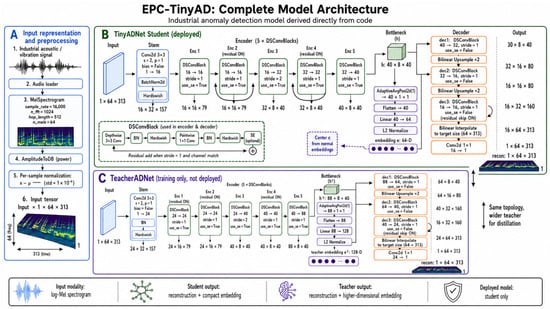
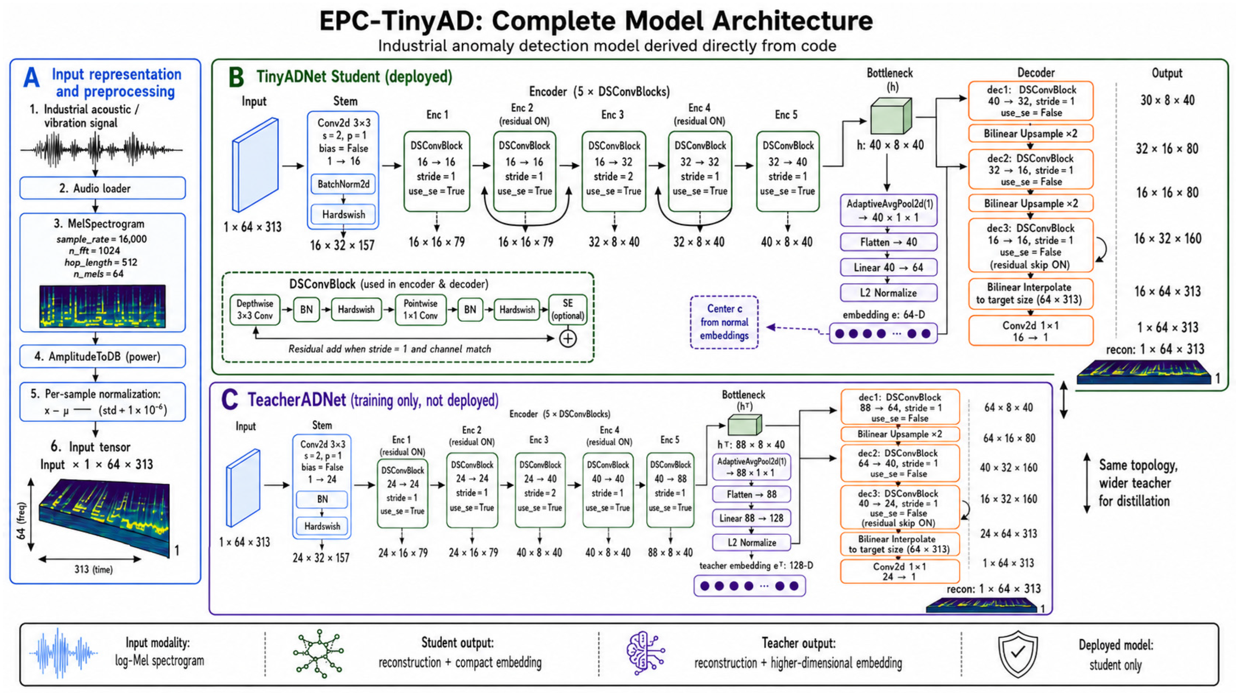
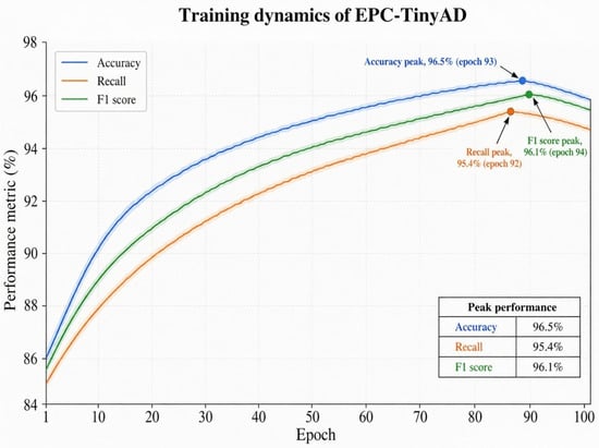
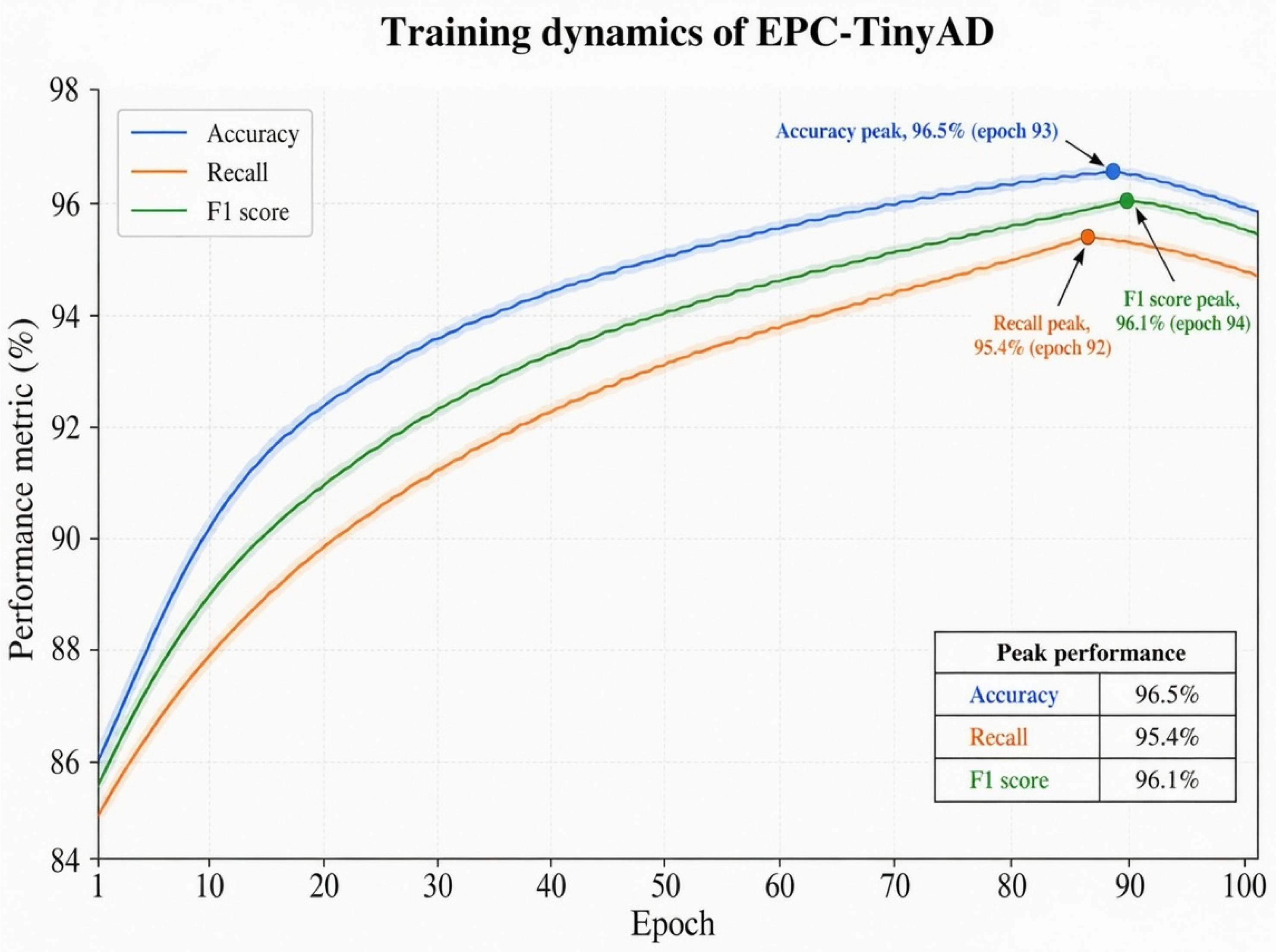
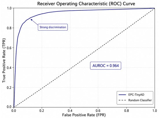
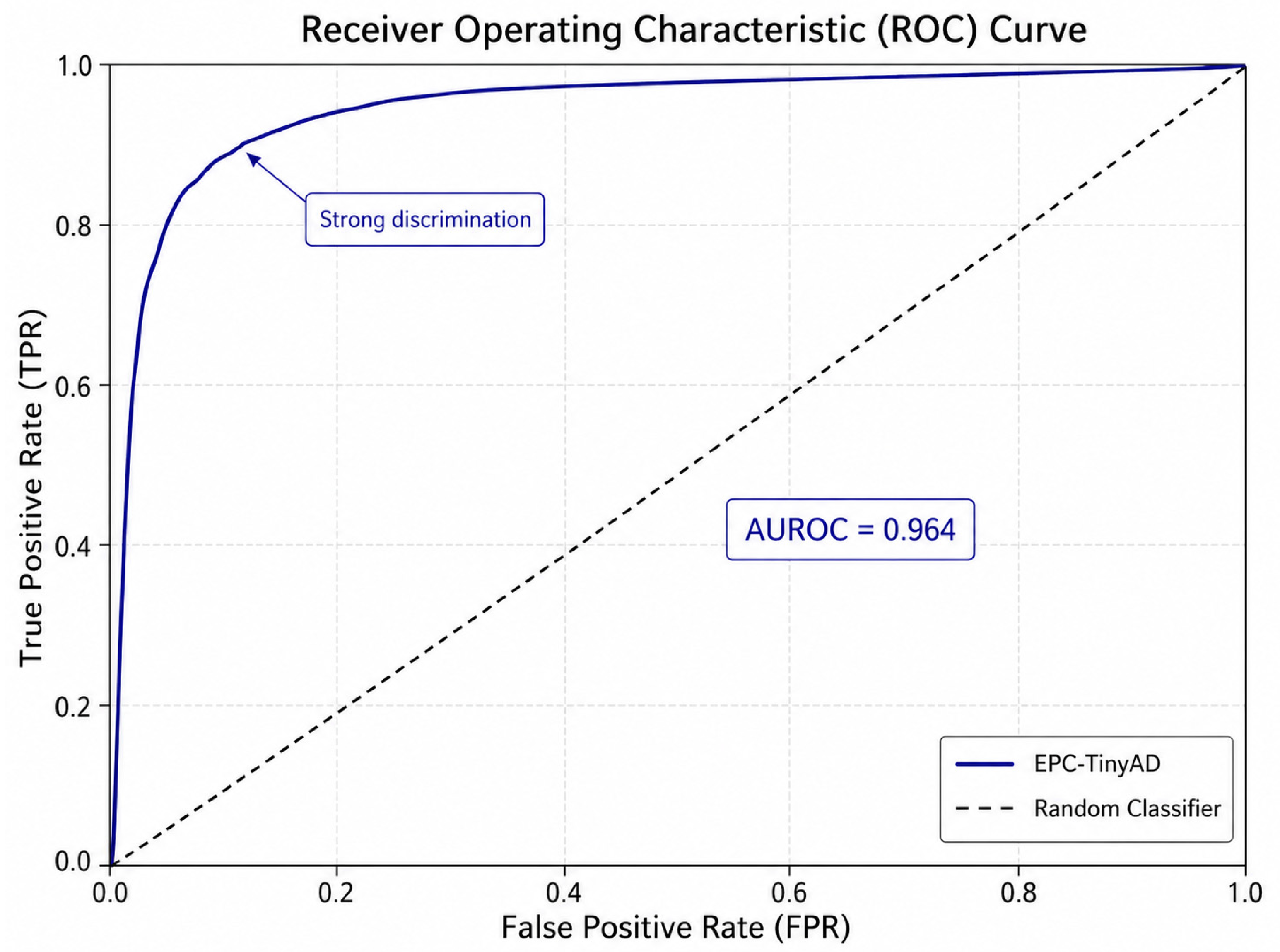
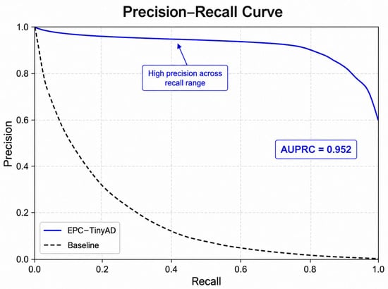
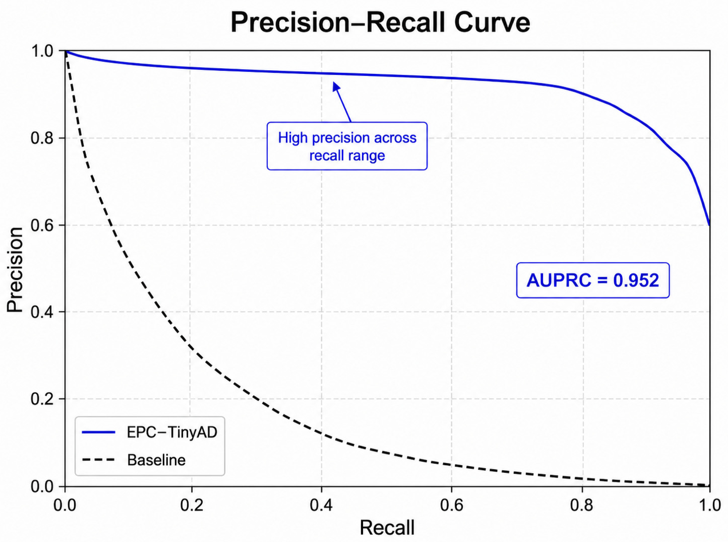
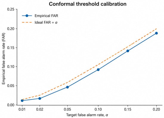
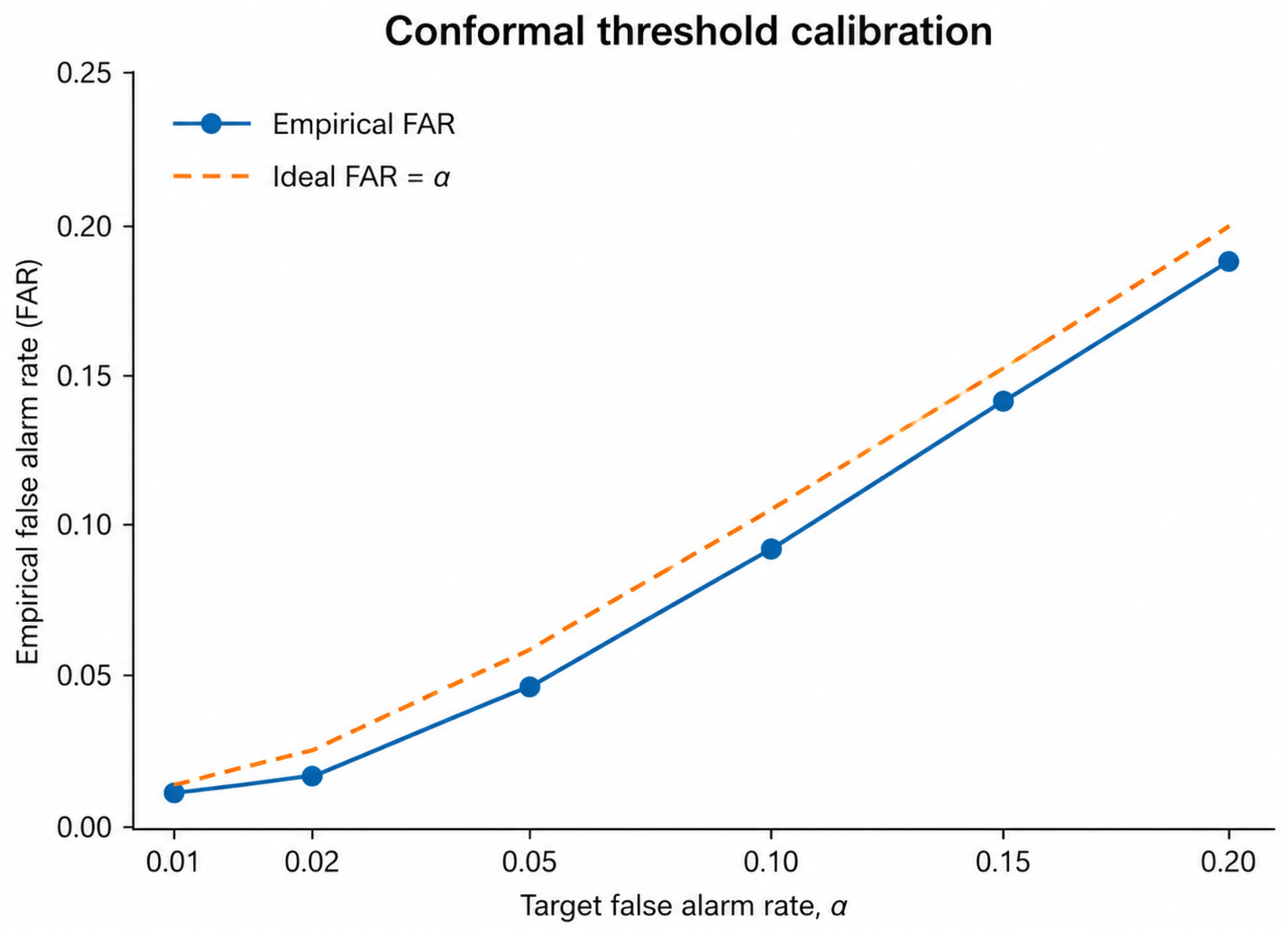
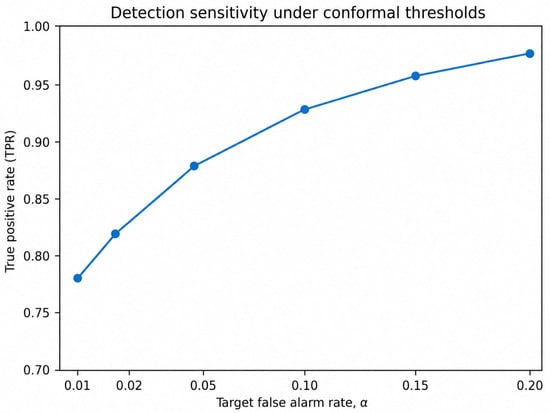
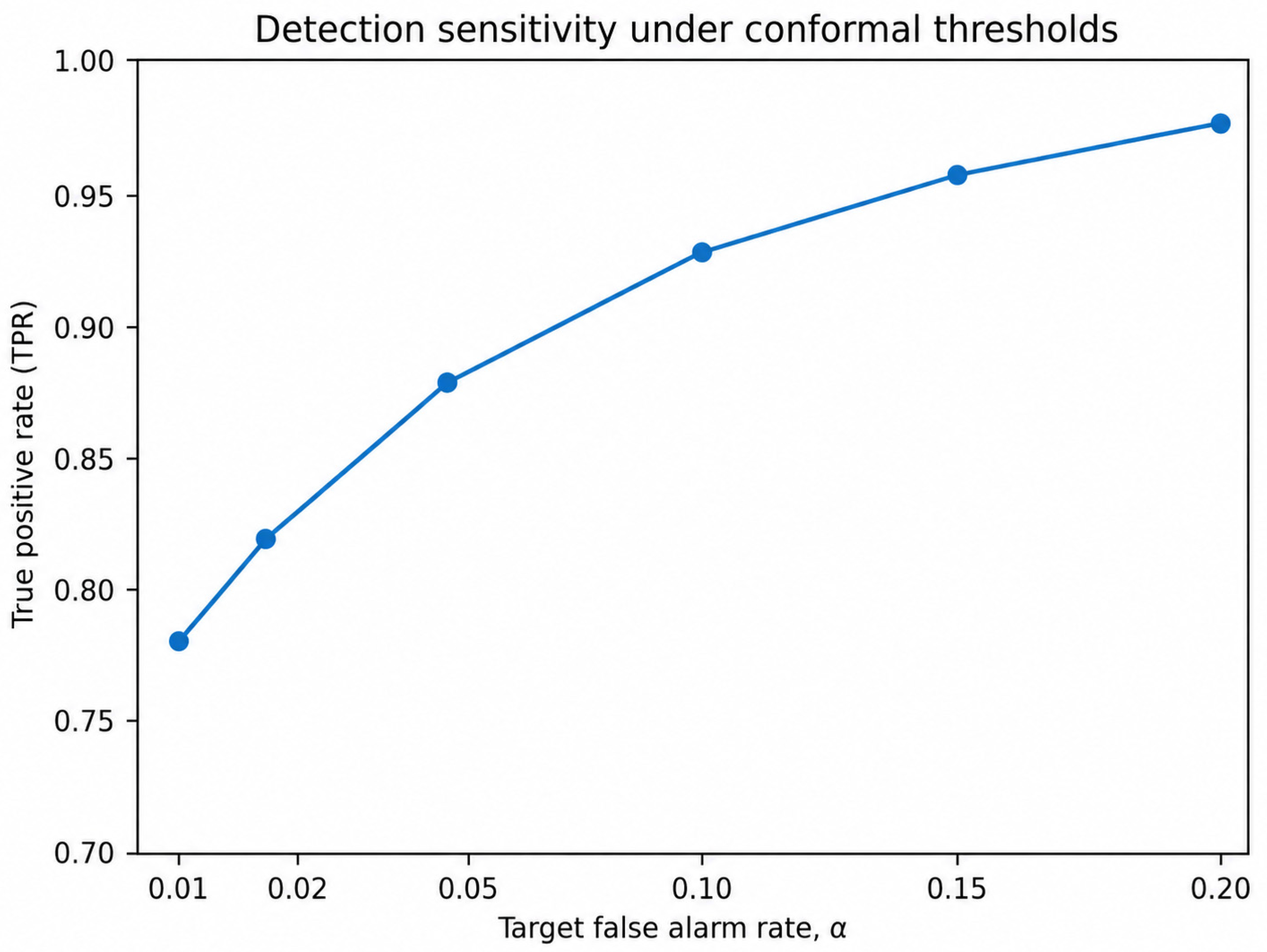
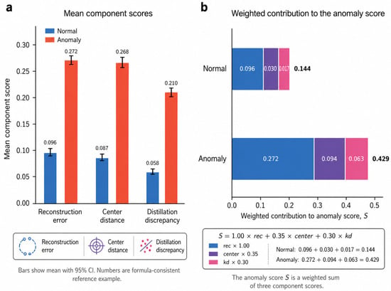
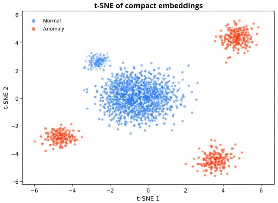
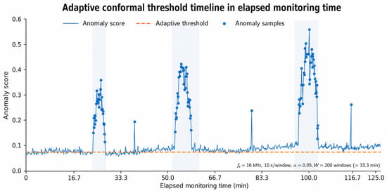
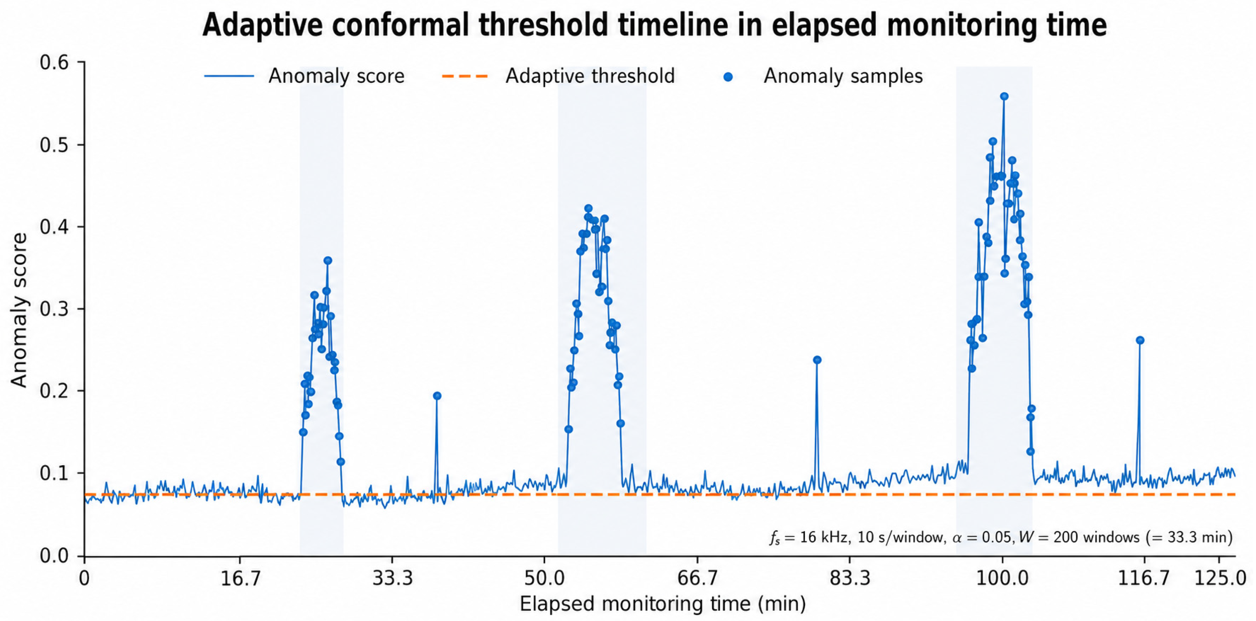
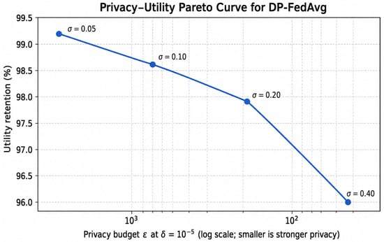
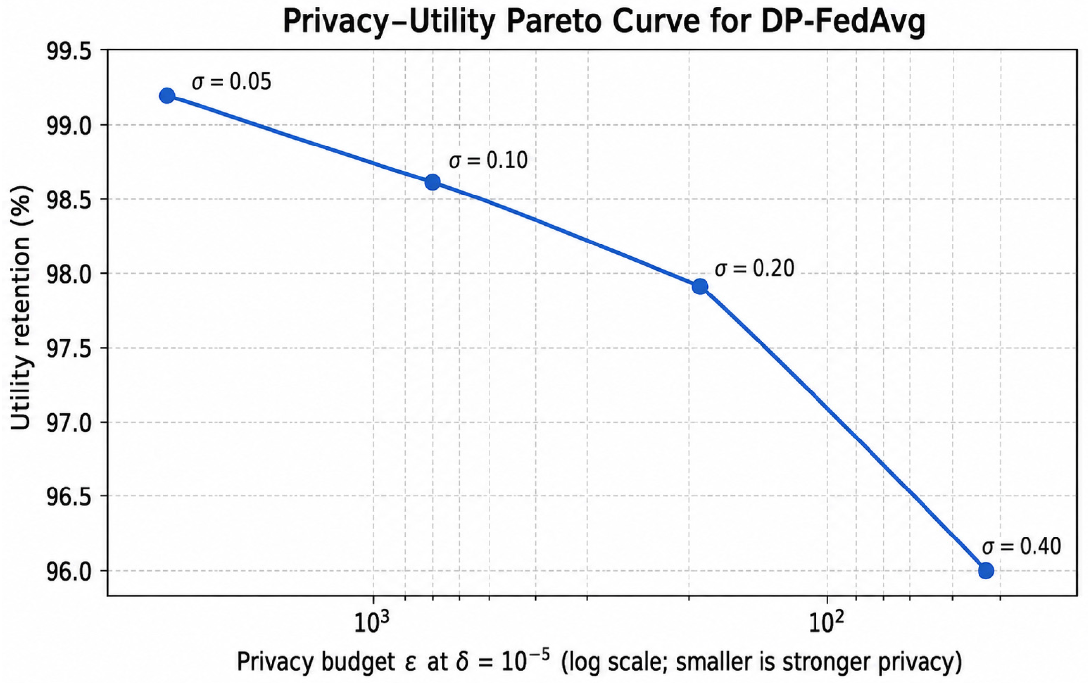

Disclaimer/Publisher’s Note: The statements, opinions and data contained in all publications are solely those of the individual author(s) and contributor(s) and not of MDPI and/or the editor(s). MDPI and/or the editor(s) disclaim responsibility for any injury to people or property resulting from any ideas, methods, instructions or products referred to in the content. |
© 2026 by the authors. Licensee MDPI, Basel, Switzerland. This article is an open access article distributed under the terms and conditions of the Creative Commons Attribution (CC BY) license.