Flexible Light Field Reconstruction: Enabling Arbitrary Sampling and Angular Resolution

Abstract

Compared with hardware-dependent methods, light field (LF) reconstruction algorithms enable a more economical and convenient acquisition of densely sampled LF (DSLF). Existing learning-based LF reconstruction methods suffer from limited flexibility, as they rely on fixed sampling patterns and predefined angular resolutions. In this paper, we propose a flexible deep learning framework, which can reconstruct DSLF with arbitrary angular resolution from randomly distributed sparse input views of an arbitrary quantity. The proposed framework consists of two core stages, namely the SAI Synthesis and the LF Refinement. The SAI Synthesis adopts Plane Sweep Volume (PSV) to cope with randomly sampled input views, and leverages the Multi-Scale Attention (MSA) module to compute per-view weights for adaptive feature fusion and support arbitrary numbers of input views. The LF Refinement stage integrates intermediate results and fully exploits LF parallax structures to further improve reconstruction quality. Experimental results demonstrate that our method achieves superior flexibility and reconstruction quality, and outperforms most state-of-the-art LF reconstruction methods.

1. Introduction

Light field, as a high-dimensional function describing light rays propagating through every point in all directions in free space [1,2], has significant potential for various applications such as 3D reconstruction [3,4], refocusing [5,6], depth estimation [7,8], and virtual reality [9]. DSLF are crucial for these applications, as they provide sufficient spatial-angular information to ensure smooth parallax shifts, natural focus details, and accurate scene geometry representation. However, acquiring DSLF directly through hardware devices like a camera array [10] or specialized LF camera [11,12] faces significant challenges. The former is bulky and expensive, and the latter suffers from inherent trade-off between spatial and angular resolution due to sensor limitation. To mitigate the limitations associated with direct acquisition, the computational reconstruction of DSLF from a sparsely sampled one has emerged.

In recent years, deep learning has yielded remarkable performance across various computer vision tasks including moving object segmentation [13], action recognition [14] and image restoration [15], and has also significantly promoted the development of light field reconstruction. Nevertheless, most existing deep learning models in LF reconstruction suffer from limited flexibility, as they adopt fixed sampling patterns and only support predefined input and output angular resolutions. Consequently, any variation in input or output resolution necessitates training a separate model, leading to high computational and limited adaptability. Moreover, when faced with randomly sampled input views, these methods often suffer from severe aliasing, blurring, or geometric inconsistency, as they fail to fully model the arbitrary relationship among views.

The Multi-Plane Image (MPI), proposed by Zhou et al. [16], is a scene representation method that enables an arbitrary angular resolution output. By blending transformed MPI from neighboring views, it can synthesize novel views at any camera position. Subsequent works by Mildenhall et al. [17], DuVall et al. [18] and Flynn et al. [19] also proposed MPI-based view synthesis algorithms. Li et al. [20] and Xiang et al. [21] designed frameworks incorporating meta-learning for LF reconstruction with arbitrary scale upsampling. Despite supporting arbitrary angular resolution reconstruction, these methods fail to accommodate input views with flexible sampling patterns and quantities. Jin et al. [22] used Plane Sweep Volume (PSV) as input for disparity estimation, thereby overcoming the constraint of fixed sampling patterns. However, this method fails to accommodate an arbitrary number of input views.

In this paper, we propose a novel deep learning framework for LF reconstruction with remarkable flexibility. Our method can reconstruct DSLF with arbitrary angular resolution from randomly distributed sparse input views of a variable quantity. Specifically, this model consists of two core stages, namely the SAI Synthesis and the LF Refinement. In the first stage, the network generates SAIs for each target viewpoint individually. Following Jin et al. [22], the first stage adopts PSV as input to encode positional relations between sparse inputs and targets, supporting arbitrarily distributed sparse views. To accommodate arbitrary numbers of input views, our network avoids dimension conversion between angular views and feature channels to preserve a standalone angular dimension. For adaptive aggregation of multi-view features, we propose the Multi-Scale Attention (MSA) module. It computes attention weights to quantify the contribution of each input view and fuses all view features dynamically using these weights. An internal Multi-scale Large Kernel Convolution (MLKC) is embedded inside the MSA module to extract multi-scale spatial-angular features. The second phase integrates all intermediate SAI information to improve reconstruction quality, with its core lying in the full exploitation of the characteristics of LF parallax structures. It leverages the MSA module to adaptively aggregate multi-view warped light fields and employs pseudo-4D convolutions for spatial-angular feature extraction.

In summary, the main contributions of this paper are as follows:

• We propose a flexible light field reconstruction framework that supports one-time training for universal adaptation. It accommodates arbitrary sampling positions and variable input view numbers, and enables outputs with arbitrary angular resolutions, effectively eliminating the fixed input–output limitations of conventional methods.
• We propose an adaptive fusion module MSA for light field feature fusion. Inside the MSA, the embedded MLKC employs multi-scale 3D convolutions to simultaneously extract spatial texture details and cross-view angular parallax features. Based on these features, MSA generates angular attention weights and fuses information from all $K$ input views.
• Extensive experiments on synthetic and real-world datasets validate the effectiveness and generalization of the proposed approach against classic mainstream light field reconstruction methods.

The rest of this paper is organized as follows. Section 2 presents a comprehensive review of existing methods for LF reconstruction. Section 3 elaborates on the proposed method in detail. In Section 4, we conduct extensive experiments to evaluate the performance of the proposed method. Finally, Section 5 draws the conclusions of this paper.

2. Related Work

LF angular super-resolution, aiming to reconstruct DSLF from sparse inputs, has attracted extensive attention for tackling core challenges in LF acquisition and application. Existing methods for LF reconstruction are mainly categorized into disparity-dependent methods and disparity-independent methods based on whether disparity maps are explicitly utilized.

2.1. Disparity-Dependent Methods

Disparity-dependent methods rely on geometric constraints between views, adopting a workflow of disparity estimation, view warping, and refinement. Among traditional approaches, Pearson et al. [23] proposed a layer-based model utilizing multiple depth layers to characterize scene geometry, which enables the synthesis of novel views at arbitrary angular positions from several given views. Wanner and Goldluecke [24] developed a variational framework, leveraging EPI images for disparity estimation and minimizing an objective function to reconstruct the LF. Zhang et al. [25] introduced a phase-based approach that infers LF disparity through a disparity-assisted phase synthesis strategy, with the estimated disparity guiding the warping of input views to realize novel view synthesis.

With the development of deep learning, CNN-based methods have become mainstream. Kalantari et al. [26] pioneered the application of sequential CNNs in LF reconstruction, dividing the process into disparity and color estimation. Shi et al. [27] designed a hybrid network that acquires depth maps through a lightweight optical flow estimation network, deploys separate reconstruction modules in the pixel and feature domains, and fuses outputs via a soft mask. Jin et al. proposed multiple improved networks, including a geometry-aware model for sparse LFs with large baselines [28], a PSV-based method for LF reconstruction from flexible sampling inputs [22]. Liu et al. [29] and Chen et al. [30] proposed fusion frameworks that combine LF images from explicit- and implicit-depth-based reconstruction. These methods dynamically balance the contributions of the two pipelines, effectively improving reconstruction performance in both large and small disparity regions while alleviating the limitations of single-pipeline methods. Ko et al. [31] proposed a trainable disparity estimator to extract multi-view features, alongside an adaptive module for remixing features from warped views. Meng et al. [32] tackled occlusion by computing aperture disparity maps, integrating a confidence map into warping to mitigate pixel occlusion during view synthesis.

2.2. Disparity-Independent Methods

Disparity-independent methods eliminate the need for explicit disparity estimation, instead directly modeling high-dimensional LF dependencies. Among traditional approaches, Mitra et al. [33] proposed a patch-based method integrated with a Gaussian mixture model (GMM) for LF angular reconstruction. Shi et al. [34] formulated the task as a sparse optimization problem in the continuous Fourier domain, utilizing boundary and diagonal views as input. Vagharshakyan et al. [35] developed an iterative regularization algorithm that leverages the sparse representation of EPIs in the discrete shearlet transform domain to achieve dense LF generation.

Recently, deep learning-based methods have achieved promising results. Yeung et al. [36] proposed a method that alternately performs feature extraction on sub-aperture images and macro-pixel images. Yoon et al. [37,38] designed cascaded CNNs to simultaneously upsample spatial and angular resolutions. Wang et al. [39] constructed pseudo-4D convolution using 2D and 3D convolutions to recover high-frequency details. Focusing on EPI features, Wu et al. [40] proposed a “blur-restoration-deblur” strategy to mitigate spatial-angular information asymmetry. In their following studies, they [41] introduced SAA-Net, a UNet-like architecture based on 3D convolutions with asymmetric kernel sizes and non-local attention, that is designed for reconstructing high-resolution EPIs. Later in [42], they presented a unified framework to implement anti-aliasing reconstruction on EPIs. Very recently, Wang et al. [43] proposed a novel EPI-guided network to emphasize differentiated learning of EPI features.

With the booming of attention mechanisms, plenty of Transformer and hybrid CNN-Transformer solutions have been developed for light field reconstruction in recent years. Wang et al. [44] developed ViewFormer, a pure Transformer-based angular SR model, which constructs encoder–decoder architecture and generates target view-specific queries via view interpolation to exploit the cross-view geometric prior, yet its parameter and computational cost grow with varying input view numbers. Liu et al. [45] put forward GLCTNet, a hybrid convolutional Transformer network combining 3D convolution and self-attention; it couples an independent deblurring branch to eliminate reconstruction artifacts caused by inaccurate feature warping in occlusion-heavy scenes. Hua et al. [46] designed LFRTR with separated spatial and angular Transformer blocks plus dense skip connections, which respectively models intra-view texture and inter-view parallax. However, all the above methods are limited to fixed input and output configurations.

3. Proposed Method

3.1. Overview

A 4D LF can be characterized by the two-plane model, i.e., the angular plane $\mathbf{u} = \left(u, v\right)$ and the spatial plane $\mathbf{x} = \left(x, y\right)$. The propagation of a light ray can be uniquely determined by points on these two planes. Let $U = \{\mathbf{u} | \mathbf{u} = \left(u, v), 1 \le u \le M, 1 \le v \le N\right\}$ be the $M \times N$ grid distributed angular coordinates of all SAIs, and $\mathcal{L} = \left\{I_{\mathbf{u}}\in {\mathrm{R}}^{W\times H} | \mathbf{u} \subset U\right\}$ be a DSLF where $I_{\mathbf{u}}$ denotes the SAI at $\mathbf{u}$ with spatial resolution $W \times H$.

Given a sparsely sampled LF (SSLF) ${\mathcal{L}}_s=\left\{I_k, 1 \le k \le K\right\}$ composed of $K$ SAIs, whose angular coordinate set is $\mathcal{V}=\left\{V_k |{ V}_k \subset U, 1 \le k \le K\right\}$, this paper aims to synthesize novel SAIs $\mathcal{N}=\left\{I_{C_t} |{ C}_t \subset C\right\}$ on the angular coordinates $\mathcal{C}=\left\{C_t | C_t \subset U-\mathcal{V}\right\}$, thereby reconstructing a DSLF $\tilde{\mathcal{L}}$ that is as close as possible to the ground-truth DSLF $\mathcal{L}$. A key advantage is that it can adapt to arbitrary changes in the number $K$ and the sampling positions $\mathcal{V}$ of the input SAIs, and the output angular resolution $M \times N$ without retraining the model. This problem can be implicitly formulated as:

$$\tilde{\mathcal{L}}={\mathcal{L}}_s\cup \mathcal{N}=f({\mathcal{L}}_s,\mathcal{V},\mathcal{C})$$

(1)

where $f$ denotes the mapping function to be learnt.

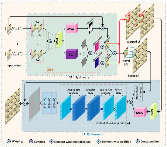
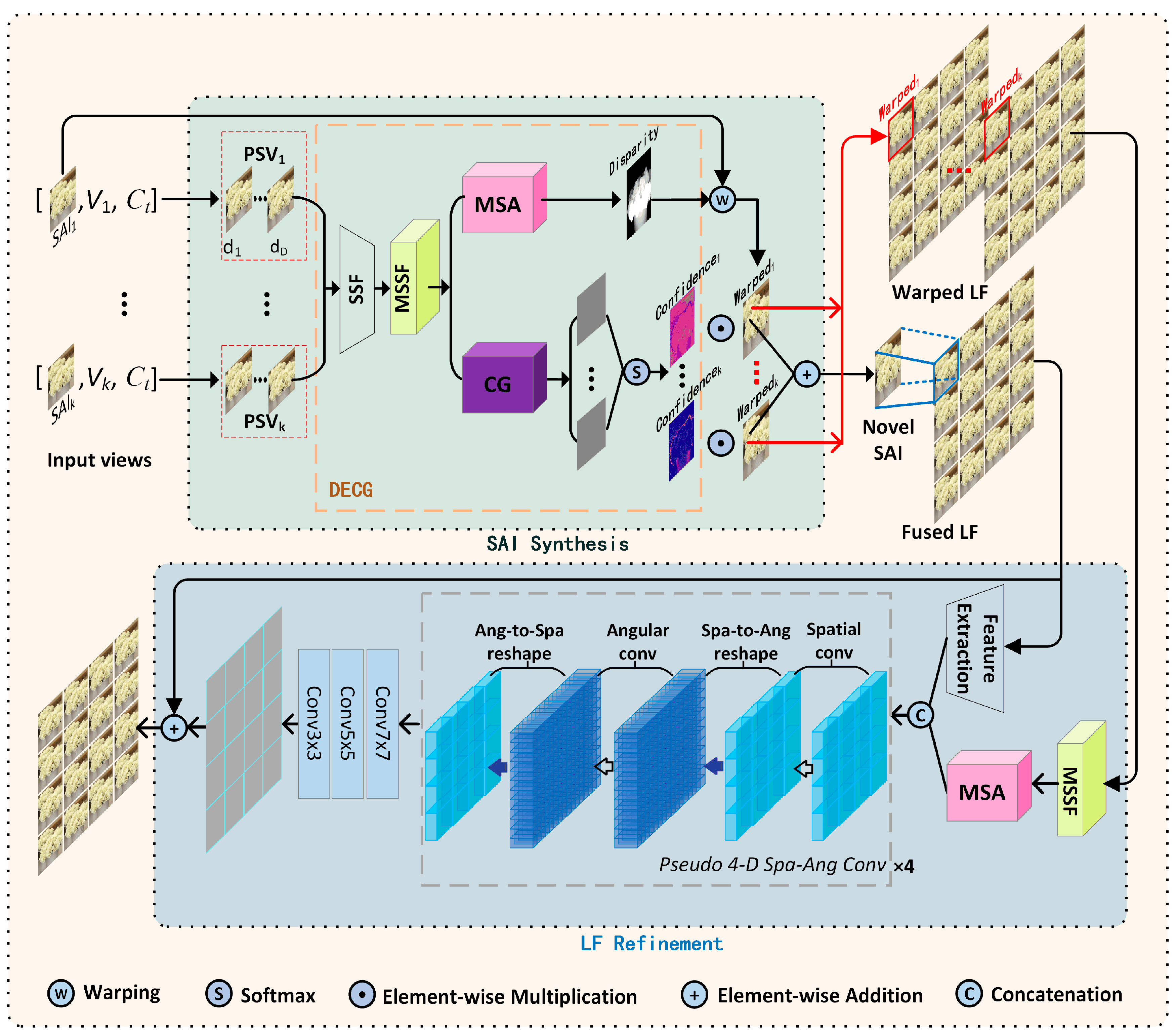
As depicted in Figure 1, our approach consists of two phases, namely the SAI Synthesis $f^s(\cdot )$ and the LF Refinement $f^r(\cdot )$. Specifically, the SAI Synthesis explicitly learns disparity information from input SAIs and warps $K$ input SAIs to produce $K$ warped images for a novel viewpoint based on the generated disparity map. Simultaneously, it generates $K$ confidence maps for the warped images and then fuses them using these maps to produce the fused SAI. This stage independently synthesizes $K$ warped images and one fused image for each novel viewpoint, where all such images across all novel viewpoints constitute $K$-warped LFs ${\mathcal{L}}_{\mathit{warp}}$ and one fused LF $\hat{\mathcal{L}}$:

$${\mathcal{L}}_{\mathit{warp}},\hat{\mathcal{L}}=f^s({\mathcal{L}}_s,\mathcal{V},\mathcal{C})$$

(2)

Figure 1. The flowchart of the proposed method. It consists of two phases, i.e., the SAI Synthesis and the LF Refinement. First, the disparity estimation and confidence generation (DECG) module generates the disparity map and confidence maps of the target viewpoint. Then, the input views are warped to the target view according to the disparity map, and the warped views are fused according to the confidence maps. Finally, the LF Refinement generates a residual map for each synthetic view that repairs its details. Specifically, spatial feature extraction (SSF) for shallow spatial feature extraction, Multi-Scale Spatial Feature extraction (MSSF) for multi-scale spatial feature exploring, and the Multi-Scale Attention (MSA) module for adaptively aggregating multi-view features weighted by confidence maps.

Then, the LF Refinement network learns residuals by exploring the complementary information between the SAIs in ${\mathcal{L}}_{\mathit{warp}}$ and $\hat{\mathcal{L}}$, aiming to recover the parallax structure of $\hat{\mathcal{L}}$. The residual maps generated by the refinement stage is added to the fused LF, yielding the final reconstructed DSLF:

$$\tilde{\mathcal{L}}=\hat{\mathcal{L}}+f^r({\mathcal{L}}_{\mathit{warp}},\hat{\mathcal{L}})$$

(3)

In the following, we will gradually elaborate on the details of the proposed method.

3.2. SAI Synthesis

This module independently generates intermediate SAIs for novel viewpoints. To handle inputs with large disparities, we leverage geometric information explicitly. Specifically, it infers the $C_t$-view disparity map and synthesizes the target SAI via backward warping. Against irregular sampling challenges, we estimate a disparity map using PSV. Meanwhile, a novel fusion strategy is proposed to support arbitrary input resolutions. In summary, the module comprises three core steps: PSV construction, disparity estimation and confidence generation, and image warping and fusion.

PSV Construction. Despite the excellent representation capability of deep learning, directly training networks with randomly sampled SAIs for novel view synthesis yields unsatisfactory performance, owing to two key limitations. Firstly, for randomly sampled SAI inputs where the angular position set $\mathcal{V}$ is intrinsically variable, it is challenging to appropriately provide the network with positional indicators related to sampling and target positions, thereby impairing prediction reliability. Secondly, view synthesis requires correlating potentially distant pixels in source images, which demands dense long-range connections and thus results in redundant parameters. Motivated by Jin et al. [22] we adopt PSVs in place of source images ${\mathcal{L}}_s=\left\{I_K\right\}$ as the input. A PSV corresponding to the target position $C_t$ is constructed via backward warping, which involves reprojecting the source images onto the disparity plane set $d=\left\{d_i,1\le i\le D\right\}$, thereby generating the corresponding warped images $\mathcal{P}=\left\{P_i^k\left(\mathbf{x}\right),1\le i\le D,1\le k\le K\right\}$, where $\mathcal{P}\in {\mathrm{R}}^{K\times D\times H\times W}$:

$$P_i^k\left(\mathbf{x}\right)=I_k(\mathbf{x}+d_i(C_t-V_k))$$

(4)

This process encodes the positions of input and target SAIs into the PSVs, eliminating the need for additional positional parameters. Furthermore, the number of disparity layers $D$ is predefined, and increasing $D$ reduces quantization error via smaller disparity steps. If any assumed disparity is correct and the corresponding scene region in the target image is unoccluded, the warped target image in the PSVs will match the reference image well. Additionally, epipolar constraints are easily enforced in PSVs, which eliminates the need for long-range pixel connections since each output pixel only depends on a small voxel column from each source PSV. Following the configuration of Jin et al. [22], we fixed $D=50$ to strike a balance between quantization error and network parameters and keep consistent experimental setups for fair baseline comparison.

Disparity Estimation and Confidence Generation. As illustrated in Figure 1, the PSV $\mathcal{P}\in {\mathrm{R}}^{K\times D\times H\times W}$ is fed into the shallow spatial feature extraction (SSF) module $f_{\mathit{SSF}}(\cdot )$ to extract the primitive spatial features by two sequential $3\times 3$ convolutions with channel 64:

$$F_{\mathit{SS}}=f_{\mathit{SSF}}\left(\mathcal{P}\right)$$

(5)

The $F_{\mathit{SS}}\in {\mathrm{R}}^{K\times 64\times H\times W}$ is then sent to the Multi-Scale Spatial Feature extraction (MSSF) module $f_{\mathit{MSSF}}(\cdot )$ to further extract the multi-scale features, which can be formulated as:

$$F_{\mathit{MSS}5},F_{\mathit{MSS}3},F_{\mathit{MSS}1}=f_{\mathit{MSSF}}\left(F_{\mathit{SS}}\right)$$

(6)

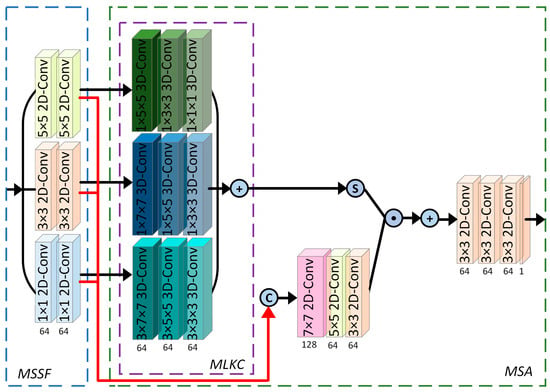
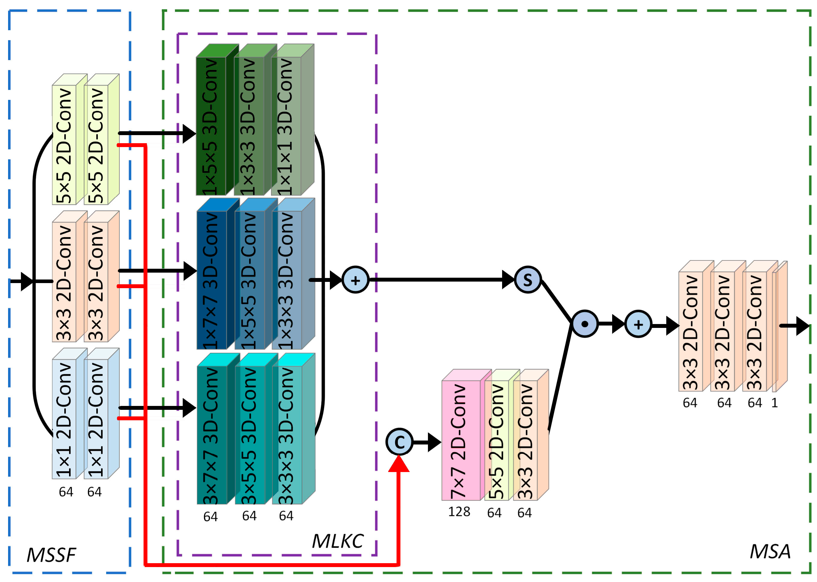
As illustrated in Figure 2, the multi-scale feature maps $F_{\mathit{MSS}5}$, $F_{\mathit{MSS}3}$ and $F_{\mathit{MSS}1}$ are respectively derived from the three branches of MSSF, each consisting of two stacked convolutional layers with kernel sizes of $5\times 5$, $3\times 3$ and $1\times 1$. To accommodate variable input counts, all feature operations in SSF and MSSF preserve the independent angular dimension $K$ without angular-channel dimension conversion. All intermediate features follow the $K\times C\times H\times W$ layout, removing the restriction of fixed input views.

Figure 2. Illustration of the Multi-Scale Spatial Feature extraction (MSSF) module, the Multi-scale Large Kernel Convolution (MLKC) module and the Multi-Scale Attention (MSA) module.

Subsequently, the multi-scale features $F_{\mathit{MSS}5}$, $F_{\mathit{MSS}3}$ and $F_{\mathit{MSS}1}$ with a uniform dimension of $K\times 64\times H\times W$ are fed into the Multi-Scale Attention module (MSA) and confidence generation (CG) module respectively to generate the target-view disparity map and the confidence maps for the $K$ warped SAIs.

As the core fusion component, the proposed MSA contains three designs: Multi for multi-branch parallel processing, Scale for multi-scale spatial-angular feature modeling, and Attention for angular-aware adaptive fusion.

First, MSA adopts the multi-scale features $F_{\mathit{MSS}5}$, $F_{\mathit{MSS}3}$ and $F_{\mathit{MSS}1}$ as parallel inputs, so as to collect multi-level spatial context and enrich feature representation from different receptive fields.

Meanwhile, MSA embeds the Multi-scale Large Kernel Convolution (MLKC) sub-module to strengthen its scale modeling capacity. MLKC executes 3D convolution over the $K\times H\times W$ dimension, which simultaneously models intra-view spatial textures and inter-view parallax correlations. Benefiting from the multi-branch architecture illustrated in Figure 2, MLKC extracts multi-scale spatial-angular features under varying $K$ and produces angular attention coefficients.

Using coefficients derived from the MLKC, the MSA carries out feature fusion in two steps. First, Softmax along the angular dimension $K$ yields per-view attention weights. Next, after concatenating $F_{\mathit{MSS}5}$, $F_{\mathit{MSS}3}$ and $F_{\mathit{MSS}1}$ along the channel axis into a $K\times 192\times H\times W$ tensor and refining features with three successive 2D convolutions, MSA multiplies the refined features by the corresponding attention weights, then sums all weighted features along the angular dimension to obtain the fused feature. This design avoids collapsing the angular dimension into channels and enables flexible arbitrary input quantities.

The processes of MSA and CG can formulated as:

$$D_{C_t}=f_{\mathit{MSA}}(F_{\mathit{MSS}5},F_{\mathit{MSS}3},F_{\mathit{MSS}1})$$

(7)

$${\mathcal{T}}_{C_t}=f_{\mathit{CG}}\left(\mathit{Con}\right(F_{\mathit{MSS}5},F_{\mathit{MSS}3},F_{\mathit{MSS}1}\left)\right)$$

(8)

where $D_{C_t}$ is the disparity map at the target view $C_t$, and ${\mathcal{T}}_{C_t}$ are the $K$ confidence maps corresponding to the $K$ warped images. The $\mathit{Con}(\cdot )$ denotes the concatenation operation along the channel dimension. The $f_{\mathit{MSA}}(\cdot )$ and $f_{\mathit{CG}}(\cdot )$ are the MSA and CG modules. Specifically, the CG module is composed of four $3\times 3$ 2D convolutional layers with kernel counts of 128, 128, 64 and 1 in sequence.

Warping and Fusion. The SAI at the target position $C_t$ can be synthesized by warping the input SAIs with the predicted disparity map $D_{C_t}$. Specifically, the image $I_{V_k\to C_t}$ obtained by warping the source image $I_k$ to the target position $C_t$ can be expressed as:

$$I_{V_k\to C_t}\left(\mathbf{x}\right)=I_k(\mathbf{x}+(C_t-V_k)\cdot D_{C_t}(\mathbf{x}\left)\right)$$

(9)

The confidence maps ${\mathcal{T}}_{C_t}$ indicate the pixel-level accuracy of the warped images from different input SAIs, thereby enabling the selection of high-precision regions for the fusion of the novel SAI. The fusion can be formulated as:

$$I_{C_t\_\mathit{fusion}}={\displaystyle {\sum }_{k=1}^K}{I}_{V_k\to C_t}\odot t_{V_k\to C_t}$$

(10)

where $t_{V_k\to C_t}\in {\mathcal{T}}_{C_t}$ is the confidence map for input SAI $I_k$, and $\odot$ is the element-wise multiplication operator.

3.3. LF Refinement

In the SAI Synthesis stage, SAIs for each target viewpoint are generated independently. This process fails to fully account for the LF parallax structure among individual SAIs, which consequently gives rise to photometric inconsistency across the SAIs within the fused LF $\hat{\mathcal{L}}=\{I_{C_t\_\mathit{fusion}} | C_t\in \mathcal{C}\}$. Therefore, in the LF Refinement stage, the parallax structure of the fused LF is further leveraged to restore photometric consistency. Additionally, this phase fully explores the inherent relationships between the warped LFs ${\mathcal{L}}_{\mathit{warp}}=\left\{I_{V_k\to C_t}\right|V_k\in \mathcal{V},C_t\in \mathcal{C}\}$, thereby further improving the reconstruction quality of DSLF. Since the core objective of LF Refinement is to rectify potential inconsistent artifacts in the fused SAIs while preserving high-frequency image textures, residual learning is specifically adopted in this module. The reconstruction LF can be obtained by Equation (3).

As shown in Figure 1, the LF Refinement adopts the MSA module introduced in disparity estimation and confidence generation to fuse the $K$ warped LFs ${\mathcal{L}}_{\mathit{warp}}$, thus adapting to the dynamically varying input number $K$. For the fused LF $\hat{\mathcal{L}}$, the network leverages four cascaded $5 \times 5$ convolutions to extract its shallow spatial features, which are then concatenated with the fused warped LF along the channel dimension. The concatenated feature maps are then fed into four cascaded pseudo 4D filters to capture joint spatial and angular information. A pseudo 4D filter approximates 4D representation via alternating spatial and angular 2D convolutions. Specifically, input features are rearranged into $F_{spa}\in R^{MN\times C\times H\times W}$, on which 2D convolution is performed over the spatial dimension to extract spatial structures. The features are then permuted to $F_{ang}\in R^{HW\times C\times M\times N}$ for subsequent 2D convolution over the angular dimension to model angular correlations. Such a design substantially reduces the computational cost of 4D convolution while retaining promising 4D feature extraction capacity, and it has been successfully adopted in various vision tasks such as 3D rendering [47], LF material classification [48], and LF spatial super-resolution [49]. With the comprehensive spatial-angular features obtained above, three layers of 2D convolution are leveraged to learn a residual map for each SAI. Finally, the residual map is added to the fused LF $\hat{\mathcal{L}}$, yielding the final reconstructed LF $\tilde{\mathcal{L}}$.

It should be noted that our framework synthesizes novel SAIs independently in the SAI Synthesis stage. In the LF Refinement stage, the pseudo 4D convolution acting on angular dimensions does not depend on the specific sizes of $M$ and $N$, thus adapting to arbitrary output angular dimensions.

3.4. The Loss Function

The loss function for network training consists of two components. First, the disparity estimation is supervised by calculating the absolute error between the warped LF images and the ground-truth ones, coupled with the $L_1$ norm of the second-order gradients of the disparity map. Meanwhile, the confidence maps are supervised by computing the absolute error between the fused LF images and the ground-truth ones, i.e.,

$${\mathcal{l}}_{\mathit{warp}}={\displaystyle {\sum }_{k=1}^K}{\displaystyle {\sum }_{t=1}^{\mathit{MN}}}{\sum }_{\mathbf{x}}\left|I_{C_t}\left(\mathbf{x}\right)-I_{V_k\to C_t}\left(\mathbf{x}\right)\right|$$

(11)

$${\mathcal{l}}_{\mathit{smooth}}={\displaystyle {\sum }_{t=1}^{\mathit{MN}}}({‖{\nabla }_{\mathit{xx}}{D}_{C_t}‖}_1+{‖{\nabla }_{\mathit{xy}}{D}_{C_t}‖}_1+{‖{\nabla }_{yx}{D}_{C_t}‖}_1+{‖{\nabla }_{\mathit{yy}}{D}_{C_t}‖}_1)$$

(12)

$${\mathcal{l}}_{\mathit{fusion}}={\displaystyle {\sum }_{t=1}^{\mathit{MN}}}{\sum }_{\mathbf{x}}\left|I_{C_t}\left(\mathbf{x}\right)-I_{C_t}^{ h}\left(\mathbf{x}\right)\right|$$

(13)

where $I_{C_t}$ is the ground-truth image in target position $C_t$, and ${\nabla }_{\mathit{xx}}$,${\nabla }_{\mathit{xy}}$, ${\nabla }_{yx}$, and ${\nabla }_{\mathit{yy}}$ denote the second-order gradients of the disparity map $D_{C_t}$ in the spatial domain. The smoothness loss ${\mathcal{l}}_{\mathit{smooth}}$ is designed to enhance the spatial smoothness of the disparity map.

Second, the reconstructed LF images are optimized by minimizing the absolute error as:

$${\mathcal{l}}_h={\displaystyle {\sum }_{t=1}^{\mathit{MN}}}{\sum }_{\mathbf{x}}\left|I_{C_t}\left(\mathbf{x}\right)-I_{C_t}^{ h}\left(\mathbf{x}\right)\right|$$

(14)

where $I_{C_t}^{ h}\left(\mathbf{x}\right)$ is the synthesized novel SAI in target position $C_t$.

Thus, our final objective is

$$\mathcal{l}={\mathcal{l}}_{\mathit{warp}}+{\mathcal{l}}_{\mathit{fusion}}+{\mathcal{l}}_h+{\lambda }_{\mathit{smooth}}{\mathcal{l}}_{\mathit{smooth}}$$

(15)

where ${\mathsf{\lambda }}_{\mathit{smooth}}$ is the weighting of the ${\mathcal{l}}_{\mathit{smooth}}$, which is empirically set to 0.001.

4. Experimental Results

4.1. Datasets and Training Details

We adopted 20 synthetic scenes from the HCI dataset [50], as well as 100 real-world light field images captured by the Lytro Illum camera from the Stanford Lytro LF archive [51] and Kalantari et al. [26] to train our network. During training, light field images were randomly and spatially cropped into $64 \times 64$ size patches and padded with zeros in all convolutional layers to preserve the spatial resolution unchanged. The proposed algorithm was implemented based on the PyTorch 2.5.1 framework and trained on an NVIDIA RTX 4090 GPU. We used the ADAM [52] optimizer with ${\beta }_1 = 0.9$ and ${\beta }_2 = 0.999$. The batch size was set to 1 due to the memory constraints, and the initial learning rate was set to 1 × 10⁻⁴ and decayed to half every 500 epochs.

We tested on both synthetic and real-world light field datasets. Synthetic tests include four scenes from HCI [50], five from HCIold [53] and 39 from Inria DLFD [54], while real-world tests consist of 70 Lytro Illum-captured LF images, covering 30scenes from [26] and the Occlusions and Reflective from [51]. We adopted the average PSNR and SSIM values across all synthetic novel SAIs to quantitatively evaluate the reconstruction quality.

4.2. Comparison with State-of-the-Art Methods

We compared our method with 4 state-of-the-art learning-based LF reconstruction algorithms, including Jin et al. [28], Jin et al. [22], Wang et al. [55], and Liu et al. [56]. Table 1 presents a comparison of these algorithms across four attributes: disparity-based status, support for flexible input sampling patterns (FIS), compatibility with flexible input numbers (FIN), and ability to generate flexible output angular resolution (FO).

Table 1. Comparison of attributes for light field reconstruction algorithms. The symbol “√” means satisfied, and “-“ means unsatisfied.

Algorithms	Dispartiy-Based	FIS	FIN	FO
Jin et al. [28]	√	-	-	-
Jin et al. [22]	√	√	-	√
Wang et al. [55]	-	-	-	-
Liu et al. [56]	-	-	-	-
Ours	√	√	√	√

4.2.1. Reconstruction Comparison with Fixed Input and Output

As shown in Table 1, the methods proposed by Jin et al. [28], Wang et al. [55] and Liu et al. [56] do not support irregular input sampling patterns. Thus, this comparison was conducted on the $2\times 2\to 7\times 7$ task, which aims to reconstruct a DSLF with $7\times 7$ SAIs from $2\times 2$ regularly distributed sparse ones. Specifically, the input SAIs are located at the four corners of the target DSLF. The corresponding results are listed in Table 2; it can be observed that:

Table 2. Quantitative results (PSNR/SSIM) of different methods for task $2\times 2\to 7\times 7$. The best results are shown in bold.

Algorithms	Jin et al. [28]	Jin et al. [22]	Wang et al. [55]	Liu et al. [56]	Ours
HCI	34.60/0.937	37.14/0.966	34.70/0.974	35.86/0.975	37.45/0.963
HCI old	40.84/0.960	41.80/0.974	42.18/0.978	41.54/0.971	42.27/0.976
Inria DLFD	34.83/0.933	37.70/0.960	36.64/0.972	36.60/0.972	38.02/0.964
30scenes	42.54/0.986	42.75/0.986	43.67/0.995	43.44/0.995	43.26/0.990
Occlusions	38.53/0.979	38.51/0.979	39.46/0.991	39.80/0.992	39.24/0.982
Reflective	38.46/0.959	38.35/0.957	39.11/0.978	39.35/0.981	38.82/0.968

• Jin et al. [28] shows the weakest performance compared to other methods, with noticeable gaps in both PSNR and SSIM.
• Disparity-independent methods, including Wang et al. [55] and Liu et al. [56], outperform disparity-dependent ones, including Jin et al. [22] and ours, in SSIM. This is likely because disparity-dependent methods rely on the accuracy of disparity estimation, and errors in this step undermine structural consistency, whereas disparity-independent methods prioritize local structural coherence by directly processing light field features.
• Jin et al. [22] and our method adopt disparity estimation and perform well on synthetic datasets with large disparities, while the methods of Wang et al. [55] and Liu et al. [56] without disparity guidance achieve better results on real-world datasets with small disparities. Synthetic data generally has ideal imaging conditions and distinct geometric features, which tends to yield relatively reliable disparity results. By contrast, real world scenes with complex occlusions and non-Lambertian surfaces may degrade disparity accuracy and introduce additional estimation errors. Disparity-free methods focus on implicit feature learning and suit scenes with small disparities better, though they may lack targeted constraints to handle large disparity effectively.
• Our method achieves better overall performance.

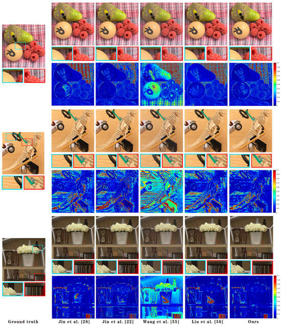
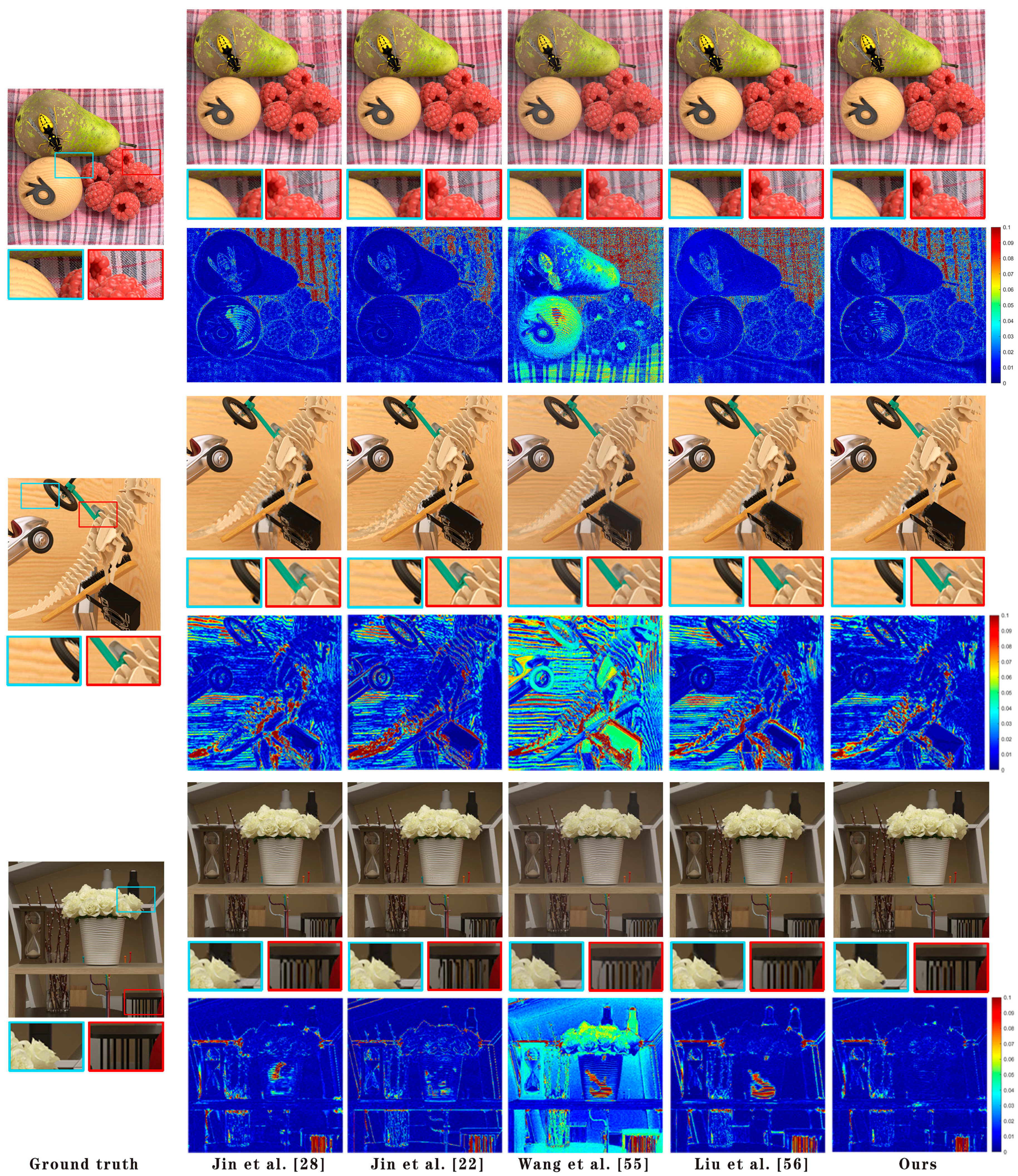
We also visually compared the reconstruction results of different methods, as shown in Figure 3. Wang et al. [55] face a challenge in handling large disparities, which is specifically reflected in the significant blurring of their reconstruction results. Our method achieves promising performance in both occluded regions and textures, such as the occluded edge of the flower and the textures on the wall.

Figure 3. Visual comparisons of different methods on the synthesized center SAI for the $2 \times 2\to 7 \times 7$ task with a fixed model. Regions outlined in red and blue boxes are magnified for clearer comparison, and we recommend viewing the figure by zooming in.

4.2.2. Reconstruction Comparison with Flexible Sampling Input

Our method supports highly flexible light field reconstruction settings. It accepts arbitrary input numbers $K\ge 1$ with no upper limit and allows input views to be located at random angular positions on the output $M\times N$ grid. It also theoretically supports reconstruction with any regular $M\times N$ output angular resolution. In contrast, the method of Jin et al. [22] only supports flexible input positions but cannot adapt to arbitrary input numbers. Therefore, we compared the reconstruction performance of the two methods over flexible sampling positions.

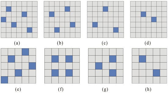
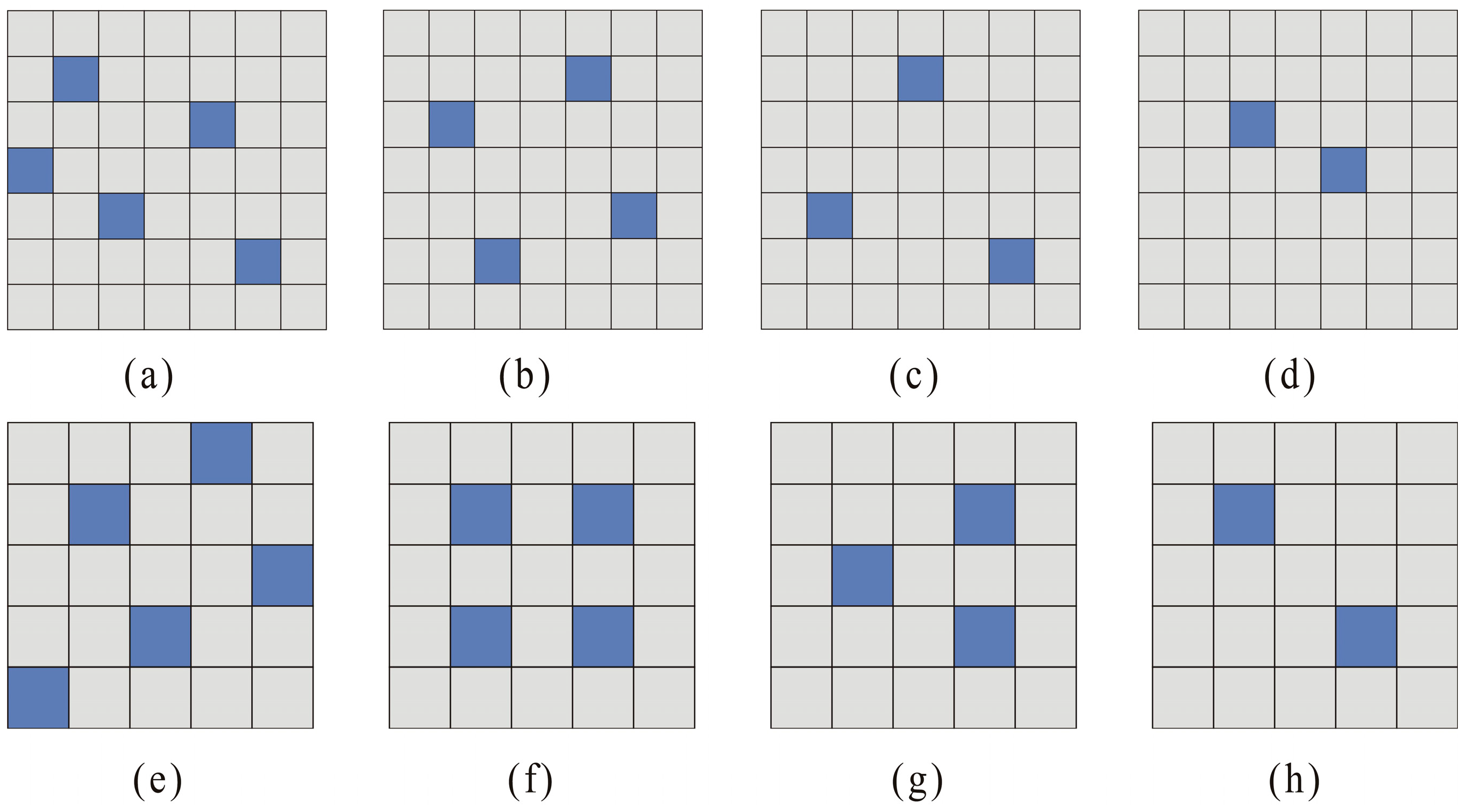
We trained a model $K\to 7 \times 7$, supporting arbitrary sampling patterns and numbers. During training, $K$ is randomly selected from 2–7, with $K$ sampling points chosen from 0–48. Despite training constraints of input $K\le 7$ and output fixed at $7\times 7$, the model still supports arbitrary input and output resolutions. The model proposed by Jin et al. [22] only supports flexible input positions but not arbitrary input numbers, so specific models for $4\to 7\times 7$, $3\to 7 \times 7$ and $2\to 7 \times 7$ tasks were trained based on arbitrary sampling positions. Quantitative results for these tasks are reported in Table 3. Each task was tested with sampling patterns shown in Figure 4: (b) for $4\to 7 \times 7$, (c) for $3\to 7 \times 7$ and (d) for $2\to 7 \times 7$.

Table 3. Quantitative comparisons of the proposed approach with Jin et al. [22] on the reconstruction with arbitrary sampling patterns under task $K\to 7\times 7$. The best results are shown in bold.

	$\mathbf{4}\mathbf{\to }\mathbf{7}\mathbf{\times }\mathbf{7}$		$\mathbf{3}\mathbf{\to }\mathbf{7}\mathbf{\times }\mathbf{7}$		$\mathbf{2}\mathbf{\to }\mathbf{7}\mathbf{\times }\mathbf{7}$
Test Set	Jin et al. [22]	Ours	Jin et al. [22]	Ours	Jin et al. [22]	Ours
HCI	38.68/0.971	38.79/0.966	38.43/0.970	37.29/0.956	37.02/0.963	34.82/0.941
HCIold	43.06/0.984	43.33/0.982	43.09/0.983	42.40/0.977	41.30/0.977	39.71/0.966
Inria DLFD	39.47/0.968	40.15/0.971	39.12/0.966	38.94/0.965	37.82/0.964	36.22/0.954
30scenes	42.83/0.986	43.54/0.992	42.57/0.986	42.86/0.987	40.98/0.982	40.14/0.969
Occlusions	39.57/0.981	39.89/0.985	39.12/0.980	39.17/0.980	37.08/0.971	36.54/0.967
Reflective	40.15/0.961	39.92/0.969	40.00/0.961	39.35/0.963	38.45/0.956	37.55/0.952

Figure 4. Illustration of different sampling patterns. (a–d) show tasks $5\to 7 \times 7$, $4\to 7 \times 7$, $3\to 7 \times 7$, and $2\to 7\times 7$, respectively; (e–h) show tasks $5\to 5\times 5$, $4\to 5\times 5$, $3\to 5\times 5$, and $2\to 5\times 5$, respectively.

Notably, our method does not require separate training for different input numbers, whereas comparable methods need repeated training for different tasks. Our method offers a distinct advantage in terms of training time. The results in Table 3 show that our method achieves lower reconstruction quality than the method of Jin et al. [22] on the $3\to 7 \times 7$ and $2\to 7 \times 7$ tasks, and the possible reasons are summarized as follows:

(1)

We randomly sampled input views from 2 to 7 during training. The sparse inputs with only 2 or 3 views are rarely involved in training, so the model lacks sufficient learning experience for such sparse cases.

(2)

Our model needs to adapt to various input quantities and random positions simultaneously, which balances the overall performance across different tasks but reduces the optimization accuracy for sparse input cases. In contrast, Jin et al. [22] trained an independent model for each task, which can be fully optimized for specific sparse inputs.

(3)

The performance drop may be partly attributed to the characteristics of the MSA module. The MSA module relies on abundant correlations among input views to compute view weights and fuse multi-view features. The superior performance under the fixed $2 \times 2\to 7 \times 7$ task verifies that our MSA module can effectively handle regular and ordered inputs. However, for random 2-view and 3-view inputs, the insufficient multi-view correlations may make it difficult for the MSA module to generate accurate weight distribution and fully exploit feature information, which could potentially lead to decreased reconstruction accuracy.

4.2.3. Comparison of the Inference Time

In this section, we compare the inference time and the number of parameters of the proposed method with the state-of-the-art approaches. All experiments are performed on the $2 \times 2\to 7 \times 7$ task, with a fixed output resolution of $512 \times 512$. All tests are conducted on an NVIDIA RTX 4090 GPU to ensure consistent experimental conditions and reliable comparison results.

The results in Table 4 show that the proposed method has slightly higher inference time and parameters than comparison methods. However, the proposed method adapts to various tasks without repeated training, which greatly reduces the training cost and delivers superior generalization performance.

Table 4. Comparison of inference time (in seconds) and parametric quantities for $2\times 2\to 7\times 7$ task.

Algorithms	Jin et al. [28]	Jin et al. [22]	Wang et al. [55]	Liu et al. [56]	Ours
Time	2.32 s	18.53 s	1.57 s	0.98 s	26.24 s
# Params.	1.11 M	1.54 M	2.68 M	6.63 M	8.54 M

Moreover, unlike other methods, the proposed network’s parameter count is independent of input view number $K$ and fixed in inference. All learnable weights are determined by channel dimensions and kernel sizes instead of angular dimensions. Adjusting $K$ only changes computation costs for feature aggregation and attention, with no extra parameters or structural adjustments required. This property ensures that our model maintains a constant parameter scale when adapting to arbitrary sparse input views.

4.3. The Effectiveness of the Method

Our framework can reconstruct LF with arbitrary angular resolution from any number of randomly sampled inputs. Based on the trained model $K\to 7 \times 7$ mentioned in Section 4.2, we evaluated eight different input–output configurations, namely $5\to 7 \times 7$, $4\to 7 \times 7$, $3\to 7 \times 7$, and $2\to 7 \times 7$, as well as $5\to 5 \times 5$, $4\to 5 \times 5$, $3\to 5 \times 5$, and $2\to 5 \times 5$. The corresponding sampling patterns for these configurations are illustrated in Figure 4.

Table 5 and Table 6 present the results corresponding to Figure 4a–d and Figure 4e–h, respectively. The observations are as follows:

Table 5. The quantitative results of the proposed method on the tasks $K\to 7\times 7$.

Test Set	$5\to 7\times 7$	$4\to 7\times 7$	$3\to 7\times 7$	$2\to 7\times 7$
HCI	39.22/0.970	38.79/0.966	37.29/0.956	34.82/0.941
HCIold	43.81/0.984	43.33/0.982	42.40/0.977	39.71/0.966
Inria DLFD	40.81/0.975	40.15/0.971	38.94/0.965	36.22/0.954
30scenes	43.87/0.994	43.54/0.992	42.86/0.987	40.14/0.969
Occlusions	40.24/0.988	39.89/0.985	39.17/0.980	36.54/0.967
Reflective	40.49/0.974	39.92/0.969	39.35/0.963	37.55/0.952

Table 6. The quantitative results of the proposed method on the tasks $K\to 5\times 5$.

Test Set	3 → 5 × 5	4 → 5 × 5	3 → 5 × 5	2 → 5 × 5
HCI	40.91/0.977	39.36/0.970	38.92/0.968	36.66/0.956
HCIold	45.16/0.988	43.77/0.985	43.47/0.984	41.47/0.974
Inria DLFD	42.47/0.981	40.50/0.974	40.45/0.974	38.51/0.964
30scenes	44.43/0.996	44.02/0.994	43.38/0.989	41.46/0.976
Occlusions	41.57/0.991	40.73/0.988	40.30/0.983	38.25/0.970
Reflective	41.98/0.977	40.98/0.972	40.52/0.969	38.63/0.961

• The reconstruction quality improves as the number of input views increases. This is because more input views provide richer angular information for LF reconstruction.
• The reconstruction quality for the $5 \times 5$ LF is higher than that for the $7 \times 7$ LF. This is because, for the same number of input views, a $5 \times 5$ LF exhibits smaller disparity than a $7 \times 7$ LF does.

4.4. Ablation Study

4.4.1. The Effectiveness of PSV

The proposed algorithm estimates a disparity map by constructing PSV. To validate the advantage of PSV, we designed an experiment that directly inputs the SAIs into the network. Table 7 presents the reconstruction results of the two different inputs on the task illustrated in Figure 4b, where PSV and SAI denote the algorithms using the PSV and SAI as the input of the network respectively. As shown in Table 7, the PSV-based algorithm yields a higher quality than the SAI-based one, validating the effectiveness of PSV.

Table 7. Effectiveness verification of PSV. The best results are shown in bold.

Algorithm	HCI	HCIold	Inria DLFD	30scenes	Occlusions	Reflective
PSV	38.79/0.966	43.33/0.982	40.15/0.971	43.54/0.992	39.89/0.985	39.92/0.969
SAI	30.35/0.901	34.79/0.924	32.68/0.911	36.91/0.937	33.02/0.923	33.39/0.908

4.4.2. The Effectiveness of MSA

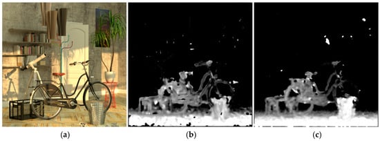
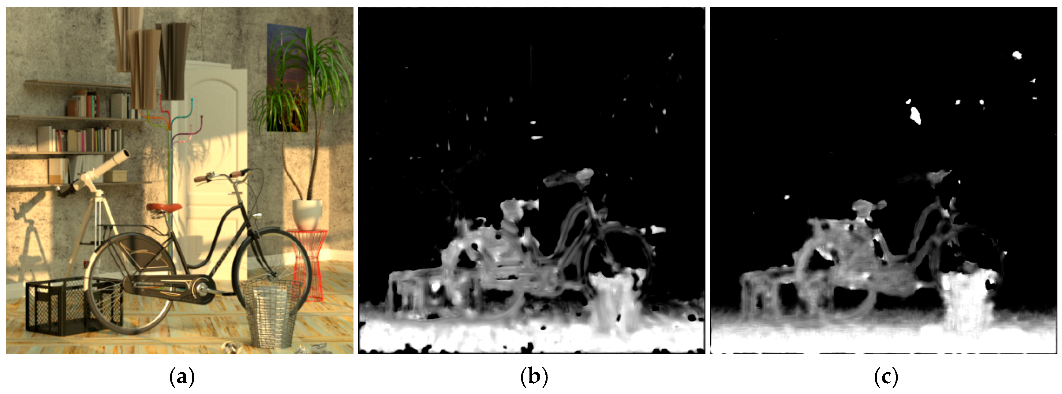
Different input SAIs provide distinct occlusion information for the target view. To fuse features from an arbitrary number of input SAIs, our method adopts the MSA fusion mechanism. To validate its effectiveness, we replaced MSA with max-pooling and trained the model under the same experimental settings. As visually compared in Figure 5, the disparity map generated by the proposed MSA-based method exhibits significantly smaller errors in background regions and occlusion boundaries than that produced by the framework using the max-pooling.

Figure 5. Visual comparisons of the disparity maps estimated by methods applying max-pooling (b) and MSA (c), where (a) presents the ground truth SAI.

4.4.3. The Effectiveness of LF Refinement

To evaluate the performance of the LF Refinement module, we quantitatively compared light field images reconstructed with and without this module, as shown in Table 8. The increase in PSNR/SSIM reveals that the module can utilize complementary information between synthesized SAIs and help improve the quality of fused light fields.

Table 8. Effectiveness verification of the LF Refinement in our approach. Specifically, w. Ref and w.o. Ref refer to the architectures with and without the LF Refinement respectively. The best results are shown in bold.

Test Set	$2 \times 2\to 7 \times 7$		$4\to 7 \times 7$
	w.o. Ref	w. Ref	w.o. Ref	w. Ref
DLFD	35.66/0.945	38.02/0.964	37.17/0.953	40.15/0.971
30scenes	40.19/0.971	43.26/0.990	40.45/0.974	43.54/0.992

5. Conclusions and Future Work

This paper proposes a flexible deep learning framework for DSLF reconstruction, which is composed of the SAI Synthesis and LF Refinement stages. The SAI Synthesis stage adopts PSV to adapt to randomly sampled inputs and uses the proposed MSA module with MLKC to adaptively calculate view weights and fuse features from arbitrary numbers of input views. The LF Refinement stage leverages light field parallax structures to further refine reconstruction quality. The proposed framework breaks the limitations of fixed sampling patterns and predefined angular resolutions, and achieves a superior reconstruction performance over most state-of-the-art methods. In future work, we will extend the framework to dynamic light field reconstruction, design lightweight network architectures for real-time inference, explore self-supervised learning strategies to reduce label dependence, and integrate multi-modal information to improve reconstruction robustness in complex scenes.

References

- Levoy, M.; Hanrahan, P. Light field rendering. In Seminal Graphics Papers: Pushing the Boundaries; ACM: New York, NY, USA, 1996; pp. 31–42. [Google Scholar]
- Gortler, S.J.; Grzeszczuk, R.; Szeliski, R.; Cohen, M.F. The lumigraph. In Proceedings of the SIGGRAPH96: 23rd International Conference on Computer Graphics and Interactive Techniques, New Orleans, LA, USA, 4–9 August 1996; Volume 96, pp. 43–54. [Google Scholar]
- Cai, Z.; Liu, X.; Peng, X.; Gao, B.Z. Ray calibration and phase mapping for structured-light-field 3D reconstruction. Opt. Express 2018, 26, 7598–7613. [Google Scholar] [PubMed]
- Zhang, J.; Yao, Y.; Quan, L. Learning signed distance field for multi-view surface reconstruction. In Proceedings of the IEEE/CVF International Conference on Computer Vision, Montreal, QC, Canada, 10–17 October 2021; pp. 6525–6534. [Google Scholar]
- Wang, Y.; Yang, J.; Guo, Y.; Xiao, C.; An, W. Selective light field refocusing for camera arrays using bokeh rendering and superresolution. IEEE Signal Process. Lett. 2018, 26, 204–208. [Google Scholar] [CrossRef] [Scilit]
- Zhang, C.; Hou, G.; Zhang, Z.; Sun, Z.; Tan, T. Efficient auto-refocusing for light field camera. Pattern Recognit. 2018, 81, 176–189. [Google Scholar] [CrossRef] [Scilit]
- Chen, R.; Sheng, H.; Yang, D.; Cong, R.; Cui, Z.; Wang, S.; Wang, T.; Zhao, M. Towards depth-continuous scene representation with displacement field for robust light field depth estimation. IEEE Trans. Multimed. 2025, 27, 3637–3649. [Google Scholar] [CrossRef] [Scilit]
- Jin, J.; Hou, J. Occlusion-aware unsupervised learning of depth from 4-D light fields. IEEE Trans. Image Process. 2022, 31, 2216–2228. [Google Scholar] [CrossRef] [Scilit] [PubMed]
- Yu, J. A light-field journey to virtual reality. IEEE MultiMed. 2017, 24, 104–112. [Google Scholar] [CrossRef] [Scilit]
- Wilburn, B.; Joshi, N.; Vaish, V.; Talvala, E.V.; Levoy, M. High performance imaging using large camera arrays. ACM Trans. Graph. (TOG) 2005, 24, 765–776. [Google Scholar]
- Lytro Illum. Available online: https://www.lytro.com/ (accessed on 1 May 2026).
- Raytrix. Available online: https://www.raytrix.de/ (accessed on 1 May 2026).
- Dong, G.; Zhao, C.; Pan, X.; Basu, A. Learning Temporal Distribution and Spatial Correlation Towards Universal Moving Object Segmentation. arXiv 2023, arXiv:2304.09949. [Google Scholar] [CrossRef] [Scilit]
- Liu, M.; Liu, J.; Jiang, Y.; He, B. Heatmap Pooling Network for Action Recognition from RGB Videos. IEEE Trans. Pattern Anal. Mach. Intell. 2025, 48, 3726–3743. [Google Scholar] [CrossRef] [Scilit] [PubMed]
- Gao, F.; Gao, C.; Deng, X.; Zhang, C.; Huang, J.; Xu, M. AIRPNet: Adaptive Image Restoration with Privacy Protection in Steganographic Domain. IEEE Trans. Pattern Anal. Mach. Intell. 2026, 48, 8148–8165. [Google Scholar] [CrossRef] [Scilit] [PubMed]
- Zhou, T.; Tucker, R.; Flynn, J.; Fyffe, G.; Snavely, N. Stereo magnification: Learning view synthesis using multiplane images. ACM Trans. Graph. (TOG) 2018, 37, 46. [Google Scholar]
- Mildenhall, B.; Srinivasan, P.P.; Ortiz-Cayon, R.; Kalantari, N.K.; Ramamoorthi, R.; Ng, R. Local light field fusion: Practical view synthesis with prescriptive sampling guidelines. ACM Trans. Graph. (TOG) 2019, 38, 29. [Google Scholar]
- Duvall, M.; Flynn, J.; Broxton, M.; Debevec, P. Compositing Light Field Video Using Multiplane Images; ACM: New York, NY, USA, 2019. [Google Scholar]
- Flynn, J.; Broxton, M.; Debevec, P.; Duvall, M.; Fyffe, G.; Overbeck, R. Deepview: View Synthesis with Learned Gradient Descent; IEEE: New York, NY, USA, 2020. [Google Scholar]
- Li, R.; Fang, L.; Ye, L.; Zhong, W.; Zhang, Q. Light field reconstruction with arbitrary angular resolution using a deep coarse-to-fine framework. In International Forum on Digital TV and Wireless Multimedia Communications; Springer: Singapore, 2021. [Google Scholar]
- Xiang, S.; Zhang, Y.; Deng, H.; Wu, J. Arbitrary-scale dense light field reconstruction with meta-learning. In Proceedings of the Chinese Control and Decision Conference (CCDC), Yichang, China, 20–22 May 2023; pp. 4394–4401. [Google Scholar]
- Jin, J.; Hou, J.; Chen, J.; Zeng, H.; Kwong, S.; Yu, J. Deep coarse-to-fine dense light field reconstruction with flexible sampling and geometry-aware fusion. IEEE Trans. Pattern Anal. Mach. Intell. 2020, 44, 1819–1836. [Google Scholar]
- Pearson, J.; Brookes, M.; Dragotti, P.L. Plenoptic layer-based modeling for image based rendering. IEEE Trans. Image Process 2013, 9, 3405–3419. [Google Scholar] [CrossRef] [Scilit]
- Wanner, S.; Goldluecke, B. Variational light field analysis for disparity estimation and super-resolution. IEEE Trans. Pattern Anal. Mach. Intell. 2013, 36, 606–619. [Google Scholar] [CrossRef] [Scilit]
- Zhang, Z.; Liu, Y.; Dai, Q. Light field from micro-baseline image pair. In Proceedings of the IEEE Conference on Computer Vision and Pattern Recognition, Boston, MA, USA, 7–12 June 2015; pp. 3800–3809. [Google Scholar]
- Kalantari, N.K.; Wang, T.-C.; Ramamoorthi, R. Learning-based view synthesis for light field cameras. ACM Trans. Graph. (TOG) 2016, 35, 193. [Google Scholar] [CrossRef] [Scilit]
- Shi, J.; Jiang, X.; Guillemot, C. Learning fused pixel and feature-based view reconstructions for light fields. In Proceedings of the IEEE/CVF Conference on Computer Vision and Pattern Recognition, Seattle, WA, USA, 13–19 June 2020; pp. 2555–2564. [Google Scholar]
- Jin, J.; Hou, J.; Yuan, H.; Kwong, S. Learning light field angular super-resolution via a geometry-aware network. Proc. AAAI Conf. Artif. Intell. 2020, 34, 11141–11148. [Google Scholar]
- Liu, X.; Wang, M.; Wang, A.; Liu, S.; Pi, X. Light field reconstruction via attention maps of hybrid networks. Vis. Comput. 2022, 39, 5027–5040. [Google Scholar] [CrossRef] [Scilit]
- Chen, Y.; Huang, X.; An, P.; Wu, Q. Enhanced light field reconstruction by combining disparity and texture information in PSVs via disparity-guided fusion. IEEE Trans. Comput. Imaging 2023, 9, 665–677. [Google Scholar] [CrossRef] [Scilit]
- Ko, K.; Koh, Y.J.; Chang, S.; Kim, C.-S. Light field super-resolution via adaptive feature remixing. IEEE Trans. Image Process. 2021, 30, 4114–4128. [Google Scholar] [CrossRef] [Scilit] [PubMed]
- Meng, N.; Li, K.; Liu, J.; Lam, E.Y. Light field view synthesis via aperture disparity and warping confidence map. IEEE Trans. Image Process. 2021, 30, 3908–3921. [Google Scholar] [CrossRef] [Scilit] [PubMed]
- Mitra, K.; Veeraraghavan, A. Light field denoising, light field superresolution and stereo camera based refocussing using a gmm light field patch prior. In Proceedings of the IEEE Computer Society Conference on Computer Vision and Pattern Recognition Workshops (CVPR Workshops), Providence, RI, USA, 16–21 June 2012; pp. 22–28. [Google Scholar]
- Shi, L.; Hassanieh, H.; Davis, A.; Katabi, D.; Durand, F. Light field reconstruction using sparsity in the continuous fourier domain. ACM Trans. Graph. (TOG) 2014, 34, 12. [Google Scholar] [CrossRef] [Scilit]
- Vagharshakya, S.; Bregovic, R.; Gotchev, A. Light field reconstruction using shearlet transform. IEEE Trans. Pattern Anal. Mach. Intell. 2018, 40, 133–147. [Google Scholar]
- Yeung, H.W.F.; Hou, J.; Chen, J.; Chung, Y.Y.; Chen, X. Fast Light Field Reconstruction with Deep Coarse-to-Fine Modeling of Spatial-Angular Clues; Springer: Cham, Switzerland, 2018; pp. 137–152. [Google Scholar]
- Yoon, Y.; Jeon, H.G.; Yoo, D.; Lee, J.Y.; Kweon, I.S. Learning a deep convolutional network for light-field image super-resolution. In Proceedings of the IEEE International Conference on Computer Vision Work-shop (ICCVW), Santiago, Chile, 7–13 December 2015; pp. 1–9. [Google Scholar]
- Yoon, Y.; Jeon, H.G.; Yoo, D.; Lee, J.Y.; Kweon, I.S. Light-field image super-resolution using convolutional neural network. IEEE Signal Process. Lett. 2017, 6, 848–852. [Google Scholar]
- Wang, Y.; Liu, F.; Zhang, K.; Wang, Z.; Sun, Z.; Tan, T. High-fidelity view synthesis for light field imaging with extended pseudo 4DCNN. IEEE Trans. Comput. Imag. 2020, 6, 830–842. [Google Scholar] [CrossRef] [Scilit]
- Wu, G.; Zhao, M.; Wang, L.; Dai, Q.; Liu, Y. Light field reconstruction using deep convolutional network on EPI. In Proceedings of the IEEE Conference on Computer Vision and Pattern Recognition (CVPR), Honolulu, HI, USA, 21–26 July 2017. [Google Scholar]
- Wu, G.; Liu, Y.; Fang, L.; Chai, T. Spatial-Angular Attention Network for Light Field Reconstruction. IEEE Trans. Image Process. 2020, 30, 8999–9013. [Google Scholar]
- Wu, G.; Liu, Y.; Fang, L.; Chai, T. Revisiting light field rendering with deep anti-aliasing neural network. IEEE Trans. Pattern Anal. Mach. Intell. 2022, 44, 5430–5444. [Google Scholar] [PubMed]
- Wang, B.; Chen, Y.; Huang, X.; An, P. A novel epi-guided network with progressive fusion for light field reconstruction. Expert Syst. Appl. 2026, 296, 128964. [Google Scholar]
- Wang, S.; Lu, Y.; Xia, W.; Xia, P.; Wang, Z.; Gao, W. Light field angular super-resolution by view-specific queries. Vis. Comput. 2025, 41, 3565–3580. [Google Scholar] [CrossRef] [Scilit]
- Liu, D.; Mao, Y.; Zuo, Y.; An, P.; Fang, Y. Light Field Angular Super-Resolution Network Based on Convolutional Transformer and Deep Deblurring. IEEE Trans. Comput. Imaging 2024, 10, 1736–1748. [Google Scholar] [CrossRef] [Scilit]
- Hua, X.; Wang, M.; Su, B.; Liu, Z.; Fan, P. Densely sampled light field reconstruction with transformers. J. Electron. Imaging 2023, 32, 033025. [Google Scholar] [CrossRef] [Scilit]
- Yan, L.; Mehta, S.; Ramamoorthi, R.; Durand, F. Fast 4D Sheared Filtering for Interactive Rendering of Distribution Effects. ACM Trans. Graph. (TOG) 2015, 35, 7. [Google Scholar] [CrossRef] [Scilit] [PubMed]
- Wang, T.; Zhu, J.; Hiroaki, E.; Chandraker, M.; Efros, A.A.; Ramamoorthi, R. A 4D Light-Field Dataset and CNN Architectures for Material Recognition; Springer International Publishing: Cham, Switzerland, 2016. [Google Scholar] [CrossRef] [Scilit]
- Yeung, H.; Hou, J.; Chen, X.; Chen, J.; Chen, Z.; Chung, Y. Light Field Spatial Super-Resolution Using Deep Efficient Spatial-Angular Separable Convolution. IEEE Trans. Image Process. 2019, 28, 2319–2330. [Google Scholar] [CrossRef] [Scilit] [PubMed]
- Honauer, K.; Johannsen, O.; Kondermann, D.; Goldluecke, B. A dataset and evaluation methodology for depth estimation on 4d light fields. In Proceedings of the Asian Conference on Computer Vision, Taipei, Taiwan, 20–24 November 2016; pp. 19–34. [Google Scholar]
- Raj, A.S.; Lowney, M.; Shah, R.; Wetzstein, G. Stanford Lytro Light Field Archive. Available online: http://lightfields.stanford.edu/LF2016.html (accessed on 1 May 2026).
- Kingma, D.; Ba, J. Adam: A Method for Stochastic Optimization. In Proceedings of the 3rd International Conference for Learning Representations, San Diego, CA, USA, 7–9 May 2015; pp. 1–13. [Google Scholar]
- Wanner, S.; Meister, S.; Goldlücke, B. Datasets and Benchmarks for Densely Sampled 4D Light Fields; The Eurographics Association: Eindhoven, The Netherlands, 2013; pp. 225–226. [Google Scholar]
- Shi, J.; Jiang, X.; Guillemot, C. A framework for learning depth from a flexible subset of dense and sparse light field views. IEEE Trans. Image Process. 2019, 28, 5867–5880. [Google Scholar] [CrossRef] [Scilit] [PubMed]
- Wang, Y.; Wang, L.; Wu, G.; Yang, J.; An, W.; Yu, J.; Guo, Y. Disentangling light fields for super-resolution and disparity estimation. IEEE Trans. Pattern Anal. Mach. Intell. 2022, 45, 425–443. [Google Scholar] [PubMed]
- Liu, G.; Yue, H.; Wu, J.; Yang, J. Efficient light field angular super-resolution with sub-aperture feature learning and macro-pixel upsampling. IEEE Trans. Multimed. 2023, 25, 6588–6600. [Google Scholar]
Disclaimer/Publisher’s Note: The statements, opinions and data contained in all publications are solely those of the individual author(s) and contributor(s) and not of MDPI and/or the editor(s). MDPI and/or the editor(s) disclaim responsibility for any injury to people or property resulting from any ideas, methods, instructions or products referred to in the content. |
© 2026 by the authors. Licensee MDPI, Basel, Switzerland. This article is an open access article distributed under the terms and conditions of the Creative Commons Attribution (CC BY) license.