


Abstract
This paper presents a time-domain analysis of an -bit pulse-width-modulated digital-to-analog converter (PWM DAC) employing a first-order passive resistor-capacitor (RC) filter. Exact analytical expressions are derived for the output settling time in both rising and decreasing digital-code transition modes. The worst-case condition is identified, and the settling-time criterion is expressed as a function of the DAC resolution , tolerance , and normalized filter parameter . The derived criterion is compared with a commonly used first-order RC settling approximation. For and , the proposed worst-case criterion gives a discrete settling interval of 823 PWM periods, whereas the literature-based estimate gives 355 periods. The analytical results are confirmed by numerical evaluation and LTspice transient simulations and are further supported by experimental measurements obtained using a microcontroller-based PWM generator and a passive RC filter. The results confirm the duty-cycle dependence of the steady-state ripple and demonstrate that the proposed criterion provides a conservative design rule for selecting PWM DAC parameters while balancing accuracy, ripple, and settling speed.
1. Introduction
In modern embedded and mixed-signal systems, it is often necessary to convert a digital signal into an analog equivalent, for example for generating reference voltages, driving actuators, forming control signals, or implementing compact sensor-interface circuits. Although dedicated digital-to-analog converters (DACs) provide well-defined static and dynamic performance, many practical systems rely on simpler and more cost-effective solutions such as the pulse-width-modulated digital-to-analog converter (PWM DAC). In this approach, a digital PWM signal is applied to a low-pass filter, producing an analog output voltage whose average value is proportional to the duty cycle ().
PWM DACs are attractive because PWM generators are available in nearly all microcontrollers, digital signal controllers, and FPGA devices, while the analog filtering stage can be implemented using inexpensive passive components, typically a resistor () and a capacitor (). Therefore, the PWM DAC architecture is widely used for generating direct-current (DC) and reference voltages [1,2], converting signals into 4–20 mA current-loop outputs for industrial transmitters [3,4], biomedical and sensor applications where PWM DACs are used to form control and measurement voltages [5], and compact mixed-signal architectures such as accelerators based on in-memory computing [6]. Recent works and technical reports also confirm the continued relevance of pulse-based DAC structures, including combined pulse-width and pulse-density digital modulators for analog signal generation [7], MCU-based PWM DAC implementations with RC low-pass filtering [8,9], and PWM-plus-filter blocks used in FPGA mixed-signal architectures [10]. In such applications, the PWM DAC provides an attractive compromise between implementation simplicity, low cost, and acceptable analog-output accuracy.
The main design difficulty of a PWM DAC is the trade-off between output ripple and settling time. A stronger low-pass filter reduces the residual ripple at the PWM frequency and its harmonics, but it also slows down the response after a duty-cycle change. Conversely, increasing the filter bandwidth improves the dynamic response but increases the steady-state ripple. Conventional design procedures usually address this trade-off in the frequency domain by selecting the filter cut-off frequency and estimating the attenuation of the PWM spectral components [1,2,11], or by using simplified first-order resistor-capacitor (RC) step-response approximations. Such approaches are useful for preliminary design, but they do not explicitly describe how the output-voltage extrema evolve within each PWM period, nor do they directly provide a conservative settling-time criterion that accounts for the PWM resolution, the digital-code transition, and the admissible ripple margin.
A time-domain formulation is therefore important when the output voltage must be guaranteed to enter and remain inside a prescribed code-dependent interval. In an -bit PWM DAC, the filtered output is not a single static value, but a periodic waveform with a finite ripple envelope around the desired quantized level. Consequently, it is not sufficient to analyze only the average value of the filtered PWM signal. The maximum and minimum values of the output voltage must also be considered, because these extrema determine whether the output remains inside the admissible range associated with a given digital code. This observation motivates the use of safe and forbidden operating zones as a design tool for connecting steady-state ripple, quantization accuracy, and transient settling behavior.
In contrast to architecture- and implementation-oriented studies, the present work develops an explicit analytical framework for the first-order RC PWM DAC. It links the steady-state ripple envelope, the per-code safe and forbidden operating zones, and the worst-case settling time to the PWM resolution and the admissible tolerance , yielding closed-form design rules rather than a specific circuit realization.
A detailed time-domain analysis of a PWM DAC with a first-order passive RC filter was previously reported in [12]. In that work, exact expressions were derived for the maximum and minimum output voltages, the average value and ripple in the steady-state condition, and the estimation of the settling time following a change in duty cycle. However, the explicit dependence of the design criterion on the PWM generator resolution , the admissible tolerance , and the worst-case digital-code transition was not fully developed. In addition, the operating-zone interpretation, which distinguishes between safe and forbidden steady-state regions, was not introduced as a systematic design metric. These aspects are essential when the PWM DAC is used as a quantized analog-output stage whose ripple must remain safely below the decision boundaries of adjacent digital codes, especially under real operating conditions where component tolerances and noise can affect conversion accuracy.
The objective of this paper is to extend the analysis presented in [12] and to provide a comprehensive and experimentally supported framework for the optimization of -bit PWM DAC structures with a first-order passive RC filter. The main contributions of this work are as follows:
- The dependence of the admissible normalized filter parameter , where is the PWM period and is the filter time constant, on the PWM resolution and tolerance is derived, providing a direct criterion for selecting the RC time constant with respect to the PWM period. Its minimum admissible value, denoted , is the smallest for which the steady-state output of every code remains within the safe operating zone, and is derived in Section 3.2.
- Safe and forbidden operating zones are introduced to define a conservative steady-state accuracy condition based on the maximum and minimum output-voltage extrema, rather than only on the average value.
- Exact time-domain settling-time expressions are derived for both rising and decreasing digital-code transitions, and the corresponding worst-case conditions are identified.
- The proposed worst-case settling-time criterion is compared with the commonly used first-order RC approximation, and the relationship between the simplified literature estimate and the present time-domain framework is clarified.
- The steady-state harmonic content at the filter output is discussed as a frequency-domain consequence of the same PWM DAC model. This provides a complementary interpretation of the residual ripple in terms of attenuated PWM harmonics.
- The analytical results are validated by numerical evaluation, LTspice transient simulations, and experimental measurements obtained using a microcontroller-based PWM generator and a passive first-order RC filter.
In this way, the paper provides a methodological tool for PWM DAC designers, offering clear insight into the trade-off between response speed and conversion accuracy. The scope of this work is intentionally limited to a first-order passive RC filter, which represents the simplest and most economical PWM DAC implementation and enables closed-form analytical expressions with clear design interpretation. Higher-order passive filters, active low-pass filters, ripple-cancelation structures [13], and generalized multi-stage architectures can further improve the ripple-settling trade-off, but they introduce additional states, component sensitivities, and implementation constraints. These extensions are therefore identified as natural directions for future work, while the first-order case analyzed here provides the reference framework and baseline design criterion.
2. Modeling of PWM DAC
The structure of a PWM-based digital-to-analog converter (DAC) consists of two fundamental parts: a digital PWM generator and a low-pass filter. The PWM generator produces a binary periodic signal, while the filter performs signal averaging and converts it into an analog output voltage. A typical block diagram of the PWM DAC is shown in Figure 1.
Figure 1.
Block diagram of the PWM DAC, consisting of a digital -bit PWM generator followed by a low-pass filter that averages the switched waveform into the analog output voltage.
In this paper, a first-order passive RC filter is considered for analytical purposes, as shown in Figure 2. This choice enables the derivation of exact analytical expressions and a straightforward interpretation of the system dynamics. More complex filters of higher order, as well as active structures, are beyond the scope of this study and may be the subject of future research.
Figure 2.
PWM DAC structure with a first-order RC filter. The PWM signal, defined by its high-level and low-level durations within the period , drives the RC network, while the output voltage charges and discharges during each period and converges toward the steady-state level determined by the duty cycle.
Figure 2 illustrates the realization of a PWM DAC with the PWM signal characterized by the high-level and low-level durations. The signal is applied to the input of a first-order RC filter whose output voltage oscillates due to the capacitor charging and discharging within each period and gradually converges toward its steady-state value. This illustrates the fundamental principle of converting a PWM signal into an analog voltage.
The PWM signal is defined by the following parameters:
- Signal period —the total duration of one PWM cycle.
- High- and low-level signal durations, and , where .
- Duty cycle .
- Voltage levels and : typically, (logical 0) and (supply voltage, logical 1).
The PWM generator is typically implemented using an -bit counter; therefore, the duty cycle can take discrete values:
where denotes the DAC resolution (number of bits), and represents the digital code.
For a quantitative description of the output-voltage behavior, we rely on the results of a detailed time-domain analysis of a PWM DAC structure with a first-order RC filter presented in [12]. In that study, general expressions were derived for:
- The maximum and minimum output voltages in the -th period:
- The steady-state (stationary) maximum and minimum values (, and digital domain transition ):
These expressions are fundamental for defining the safe and forbidden operating zones of the PWM DAC, as well as for the analytical determination of the settling time.
Steady-State Harmonic Interpretation
The main analysis in this paper is performed in the time domain, because the proposed accuracy and settling-time criteria are based on the maximum and minimum values of the filtered PWM waveform. Nevertheless, the same first-order PWM DAC model can also be used to determine the steady-state harmonic components at the output of the RC filter. This provides a frequency-domain interpretation of the residual ripple and is consistent with conventional PWM DAC design approaches based on the attenuation of PWM spectral components [1,2,11].
In the steady state, the filtered output is a periodic waveform with the PWM period . The duty cycle is denoted by , and for the -bit PWM DAC considered in this paper it is given by Equation (1), . The steady-state extrema of this periodic waveform are given by Equations (4) and (5). Therefore, the following frequency-domain interpretation refers to the same steady-state waveform, but it is used only to describe its harmonic content.
The average, or DC, component of the PWM DAC output is:
For the ideal unfiltered PWM waveform with voltage levels and , the magnitude of the -th complex Fourier coefficient, is:
The -th PWM harmonic occurs at the angular frequency , where is the fundamental PWM angular frequency. The magnitude of the first-order RC filter transfer function at this harmonic frequency is:
where is the filter time constant and is the dimensionless normalized filter parameter. The limiting value , derived later from the safe-zone criterion, represents the admissible boundary value of this parameter.
Consequently, the magnitude of the -th complex Fourier coefficient at the RC filter output is:
This expression has a direct physical interpretation. The first factor represents the -th harmonic component of the ideal unfiltered PWM waveform expressed by Equation (7), while the second factor represents the attenuation introduced by the first-order RC filter at the same harmonic frequency expressed by Equation (8). Therefore, in the ideal first-order passive RC model considered in this paper, the steady-state ripple can be interpreted as the residual contribution of attenuated PWM harmonic components at the filter output.
It should be noted that denotes a complex Fourier coefficient. Therefore, the corresponding one-sided sinusoidal amplitude of the -th harmonic is . The peak-to-peak ripple is obtained from the combined time-domain contribution of all harmonic components with their phases, rather than from a simple summation of magnitudes.
This frequency-domain interpretation is included only as a complementary steady-state view. It is not used as the settling-time criterion. In the following sections, the analysis remains based on the output-voltage extrema and the corresponding safe operating zones.
3. Definition of Operating Zones of PWM DAC
This chapter analyzes the operation of the PWM DAC with a first-order RC filter, with the aim of clearly defining the safe, transitional, and forbidden operating zones. The boundaries of these zones are determined based on the analytical expressions for the maximum and minimum output voltages, as well as the quantized transfer function with the quantization step .
In this way, a precise criterion is established for distinguishing between stable and unstable operating regimes. The results are graphically illustrated through figures that clearly separate the safe and forbidden regions, as well as the transitional zones where the system cannot reach a stable steady-state condition.
3.1. Discretization and Quantization Models
The discrete duty cycle values defined by Equation (1) form the basis for the quantization model of the PWM DAC. Since the PWM period is divided into subcycles, the duty cycle can assume only discrete values. Theoretically, the duty-cycle range is however, in practical implementations, the extreme values and are not always simultaneously used, and the operational range depends on the selected quantization convention. In this context, two standard uniform quantization conventions, mid-tread and mid-rise, are considered.
Two standard approaches are typically considered:
- Mid-tread model—the operational range is defined as:
As shown in Figure 3, the mid-tread realization illustrates three consecutive PWM periods corresponding to duty cycles , and . This representation highlights that the lower extreme () is available, whereas the upper extreme () is excluded. As a result, a short low-level interval is always present at the top end of the duty-cycle range. Consequently, even the smallest change in the digital input code causes a corresponding change in the PWM duty cycle, which in turn modifies the average value of the signal within one period. Since the RC low-pass filter follows this average component, every minimal variation in the digital code produces a corresponding change in the steady-state output voltage.
Figure 3.
PWM signal in the time domain for the mid-tread model () for three representative digital codes , and , corresponding to the duty cycles , and . The lower extreme is included, while the upper extreme , corresponding formally to , is excluded; therefore, a finite low-level interval remains even at the highest code. Horizontal axis: time normalized to the PWM period T; vertical axis: PWM output level.
- Mid-rise model—the operational range in this case is defined as:
As shown in Figure 4, the mid-rise realization illustrates three PWM periods with duty cycles , and , demonstrating that the upper extreme () is available, while the lower extreme () is excluded.
Figure 4.
PWM signal in the time domain for the mid-rise model () for three representative digital codes , and , corresponding to the duty cycles , and . In this model, the upper extreme is included while the lower extreme is excluded, so a finite high-level interval remains at the low end of the range. Horizontal axis: time normalized to the PWM period T; vertical axis: PWM output level.
As a result, at the lower end of the range, each PWM period contains at least a short high-level interval. Consequently, even the smallest change in the digital input code results in a corresponding variation in the PWM duty cycle and, therefore, in the average value of the signal within one period. In this case as well, the RC low-pass filter follows this change in the average component, which leads to a measurable shift in the steady-state output voltage.
Depending on the selected quantization model, either the lower extreme or the upper extreme of the duty-cycle range is excluded. This treatment of extremes is important in practical PWM implementations, because different timer peripherals may define the compare event and the terminal counter value in different ways. As a result, the exact mapping between the digital code and the duty cycle must always be interpreted according to the selected PWM realization.
To enable a direct comparison of the code-to-voltage mapping, Figure 5 shows a 3-bit example of the discrete transfer characteristics of a PWM DAC for both quantization models. In the mid-tread model, the quantization levels lie on the interval boundaries, whereas in the mid-rise model they are centered within the intervals.
Figure 5.
Discrete transfer characteristics of a 3-bit PWM DAC: (a) mid-tread model, where the quantization levels lie on the interval boundaries; (b) mid-rise model, where the levels are centered within intervals. Horizontal axis: digital code ; vertical axis: normalized steady-state output voltage. The blue and orange stepped lines represent the code-to-voltage mapping for the mid-tread and mid-rise models, respectively.
The discretized transfer function for code in the mid-tread model is expressed as:
where the quantization step is .
For the mid-rise model, the discretized transfer function takes the form:
In this paper, the mid-tread model is adopted for the main analysis because it is directly consistent with the duty-cycle definition introduced in Equation (1), , where the digital code takes values from 0 to . Under this convention, the lower extreme is included, while the upper extreme is excluded. This is representative of PWM counter implementations in which the duty cycle is generated by comparing an -bit counter value with a digital compare value, so that the maximum digital code still leaves a finite low-level interval within each PWM period.
The choice of the mid-tread model also simplifies the connection between the digital code, the average output value, and the steady-state extrema derived in Equations (2)–(5). The safe-zone and settling-time criteria developed in the following sections are therefore formulated using this mapping.
For a mid-rise realization, the same analytical procedure can be applied after using the corresponding shifted code-to-duty-cycle relation implied by the mid-rise model. In that case, the interpretation of extremes, code boundaries, and quantization levels are shifted with respect to the mid-tread case.
Because the worst-case settling condition occurs near , which is an interior duty cycle reachable in both models, the design criterion (the minimum admissible value of the normalized filter parameter , derived in Section 3.2) is identical for the two realizations. The half-quantization-step offset of the mid-rise grid may slightly shift the discrete code index and, consequently, the rounded discrete settling interval, depending on the selected PWM realization. The underlying first-order RC charging and discharging dynamics, and the form of the derived safe-zone and settling-time criteria, remain unchanged.
Consequently, the proposed framework is not limited to a particular timer implementation. When applying the derived expressions in practice, the designer must use the duty-cycle mapping that corresponds to the actual PWM peripheral and quantization convention.
3.2. Operating Zones
For the PWM DAC to function correctly, it is necessary that, for a given digital code , the steady-state analog output voltage remains within the range . In the ideal case, this condition ensures full coverage of the dynamic range of quantized voltage levels. However, under real operating conditions, due to unavoidable tolerances of the passive components of the RC low-pass filter (resistors and capacitors) and the presence of noise, the above requirement becomes overly relaxed.
Such an approximation may lead to situations, especially near the boundary (extreme) values of the duty cycle, where the results have no physical meaning, as the system cannot reach a stable steady-state condition without additional correction. For this reason, the analog output voltage range can be divided into safe and forbidden zones, as illustrated in Figure 6, where the safe zone for a given digital code is defined within the range , . The portion of the range not covered by the safe zones for all possible digital codes represents the forbidden regions of the PWM DAC output voltage in the steady state.
Figure 6.
Illustration of safe and forbidden operating zones: (a) operating zones of the PWM DAC for a 3-bit input, where the green bands denote the safe zones satisfying the prescribed tolerance criterion, the orange bands denote the adjacent forbidden regions outside the allowed tolerance band, and the stepped black line represents the DAC transfer characteristic for digital codes from to ; (b) detailed zone structure around an arbitrary digital code , showing the safe band in and the adjacent forbidden margins up to .
As shown in Figure 6a, the operating zones of the PWM DAC are illustrated for a 3-bit input. The green areas represent safe zones in which the steady-state output satisfies the prescribed tolerance criterion, while the orange areas denote forbidden regions in which this criterion is not satisfied. The stepped black line represents the DAC transfer characteristic, with quantization levels ranging from to .
Figure 6b shows the local structure of the zones around an arbitrary digital code . This representation illustrates the safe band around the target code and the adjacent forbidden regions, which define the range within which the PWM DAC output must remain in order to satisfy the steady-state accuracy criterion.
In the steady-state condition, as shown in Figure 7, the following conditions must be satisfied for the safe zone:
Figure 7.
Illustration of the boundary conditions used to define the safe zone. For a given code , the steady-state maximum output must not exceed the upper safe-zone boundary, and the steady-state minimum output must not fall below the lower safe-zone boundary. These two conditions yield the inequalities from which the admissible normalized filter parameter is derived.
After substituting (4) and (5) into the expressions for and , respectively, the following inequalities are obtained:
and
Before proceeding further, note that applying the substitution in Equation (17) yields Equation (16) for , meaning that the two inequalities are equivalent and it is sufficient to consider only one of them.
In Equation (16), as the parameter increases, the denominator decreases faster than the numerator, causing the left-hand side to increase. Thus, inequality provides the following condition:
The boundary value of is obtained as the solution of the equation
where the function is defined as:
To determine the worst-case operating condition, it is necessary to find the minimum of the function , which represents the lowest value of the parameter for which the PWM DAC remains within the safe operating zone. Differentiating Equation (20) with respect to therefore gives:
The condition for the critical point is , from which it follows that:
or equivalently,
By expanding the RHS term of Equation (23) into a Taylor series for small and substituting it into Equation (22), the expression for can be approximated as:
The second derivative of with respect to , for , is:
for .
For to have a minimum at , the denominator must be positive:
Using the same Taylor-series approximation applied earlier (for small values of ), inequality in Equation (26) yields:
Since is a discrete variable, it is important to determine when the local minimum lies closer to than to . This implies that the second term in Equation (24) must be:
or equivalently,
The analysis confirms that the worst-case condition for occurs when , under the conditions expressed in Equations (27) and (29).
In the subsequent analysis, these conditions are assumed valid and will later be verified for consistency.
An estimation of can be obtained from Equation (21), for :
which gives:
With the substitution , the following quadratic equation is obtained:
The solutions are:
Since the solution (i.e., ) is not physically meaningful, the valid solution is:
From this, it follows that:
The validity of the conditions given by Equations (27) and (29) can now be verified:
- : always satisfied.
- satisfied if . Since by definition , the condition is met in all practical cases.
Equation (35) shows that decreases as the DAC resolution increases. This means that higher-resolution PWM DAC operation requires a smaller normalized filter parameter , i.e., stronger low-pass filtering relative to the PWM period. Consequently, the improvement in steady-state accuracy is obtained at the cost of a longer settling interval. The tolerance directly influences the width of the safe zone—a larger tolerance increases the allowable range around the target code but relaxes the required settling accuracy.
In addition to the dependence of on and , the approximation errors arising from the use of the simplified expression for estimating are also analyzed. The simplified approximation is compared with the exact analytical value:
Both the relative and absolute approximation errors are considered.
Figure 8 shows the dependence of the exact analytical value (, expressed in Equation (36)) on the number of bits for several typical tolerance values, and . These values are selected because they are below the maximum permissible limit , ensuring operation within the prescribed safe-zone tolerance.
Figure 8.
Exact limiting admissible normalized filter parameter as a function of the number of bits , obtained from Equation (36). The three curves correspond to the tolerance values and . Horizontal axis: number of bits ; vertical axis: , the limiting value of at which the safe-zone criterion is satisfied. The decrease of with shows that higher-resolution PWM DACs require a smaller normalized filter parameter, i.e., stronger low-pass filtering relative to the PWM period, for the same settling tolerance.
Figure 9 shows the relative approximation error of the parameter , defined as:
Figure 9.
Relative approximation error of the parameter , defined as the relative difference between the simplified design rule from Equation (35) and the exact value from Equation (36), expressed in percent. The curves correspond to and . Horizontal axis: number of bits ; vertical axis: relative error [%]. The error decreases rapidly with increasing , confirming that the simplified rule is highly accurate over the practical resolution range.
Figure 10 illustrates the absolute error:
Figure 10.
Absolute approximation error of the parameter , defined as the absolute difference between the simplified design rule from Equation (35) and the exact value from Equation (36). The curves correspond to and . Horizontal axis: number of bits ; vertical axis: absolute error in the dimensionless parameter . The error decreases monotonically with increasing resolution.
For both error metrics shown in Figure 9 and Figure 10, the curves are plotted for three typical tolerance values, and . Both the relative and absolute approximation errors decrease with increasing number of bits , confirming that the simplified expressions become more accurate for higher-resolution DACs.
The validity range of the simplified design rule can also be stated analytically. The approximation in Equation (35) is obtained by retaining the leading term of the series expansion used to simplify the exact expression. The ratio of the first neglected term to the retained leading term gives the following estimate of the relative approximation error:
This expression shows that the accuracy of the simplified rule depends only on and , and improves rapidly with increasing resolution. In the practical range considered in Figure 9 and Figure 10, and for the general admissible tolerance range , the estimated relative error remains below approximately , reaching this maximum only at the lowest resolution and at the limiting tolerance . For , the estimated relative error falls below over the same tolerance range.
Therefore, the simplified expression can be used as a compact design rule across the considered practical range of resolutions and tolerances, in agreement with the numerical results shown in Figure 9 and Figure 10. If the expression is extrapolated to the extreme theoretical case and , the estimated relative error remains below approximately . However, for such very low-resolution limiting cases, the exact expression in Equation (36) should be used.
It is also important to analyze the position of the critical point , where the function reaches its minimum, since this point defines the boundary condition for stable system operation.
Figure 11 shows the deviation error of the critical-point position , as derived in Equation (24), relative to the assumed value , for different values of the bit number .
Figure 11.
Deviation of the critical-point position from the central reference code used in the worst-case approximation. The plotted quantity is , expressed in LSB, for and . Horizontal axis: number of bits ; vertical axis: critical-point deviation []. The small magnitude of the deviation, which remains well below one over the considered range, shows that the critical point is close to the central code and supports the approximation used in the subsequent settling-time analysis.
Based on the approximation of the critical point given in Equation (27), the second term in the expression represents a correction of the critical-point position that depends on the tolerance (since from Equation (35)). For typical values , the contribution of this term is smaller than one quantization step (1 ), and can therefore be considered negligible in further calculations, as confirmed by the results in Figure 11.
Consequently, to simplify the expressions, the critical point can be approximated without significant loss of accuracy such as:
which confirms the initial assumption that the worst-case condition for occurs approximately at .
After considering the error in the position of the critical point, the next step in analyzing the PWM DAC structure is to examine the margins, i.e., the distance between the maximum and minimum steady-state output voltages and the boundaries of the safe zone for a given code .
The analysis of the maximum margin is performed by defining the function :
where the distance between and the boundary of the safe zone is normalized with respect to the quantization step
By substituting the known expression given by Equation (4) for the steady-state output voltage , the margin function becomes:
To find the point of minimum of the margin, the first derivative of the function is calculated:
By setting , the critical point is obtained:
Hence,
The second derivative confirms that the point corresponds to a minimum:
for , indicating that the function is convex.
Using relation given by Equation (44) in Equation (42), the analytical expression for the lower bound of the maximum margin is obtained:
Substituting yields:
After determining the lower bound of the maximum margin, it is also necessary to examine the behavior of the margin at the boundaries of the digital input range, i.e., for and . These boundary points represent extreme cases, and it is essential to verify that the margin remains within the prescribed tolerance .
For :
which represents the maximum possible margin value and thus satisfies the condition that the margin does not exceed .
For :
confirming that the condition is met.
Figure 12 presents the results of the numerical analysis of the maximum margin function for various and tolerance values .
Figure 12.
Maximum margin function across the digital input range, evaluated for the optimal boundary value . The horizontal axis is the normalized digital code , and the vertical axis is the normalized maximum margin , expressed in . For each tolerance level and (dashed horizontal lines), a separate group of curves is shown for and . Within each group, the curves for different nearly coincide because of the normalized representation, with the green curve (), drawn last, appearing dominant in the overlapping regions. In every case the curves reach but do not exceed the corresponding line, confirming that the upper-boundary condition is satisfied over the complete code range.
From the presented graph, it can be concluded that the condition is satisfied throughout the entire digital input range .
After examining the maximum margin, the next step is to determine the minimum margin of the output signal, defined as:
Differentiating Equation (51) gives:
Setting , yields the critical point :
which leads to:
i.e., the same critical point as in the maximum margin case ().
The second derivative of Equation (51) is:
confirming that the function is convex and that is indeed a minimum point.
Substituting relation expressed in Equation (53) into Equation (51) yields the analytical expression for the lower bound of the minimum margin:
confirming that the margin is identical to that in Equation (47) and remains above zero and within the permissible tolerance .
After determining the minimum point , as in the case of the maximum margin, it is necessary to verify the boundary cases for and .
Verification at :
which corresponds to the largest possible margin value and confirms that it does not exceed the allowed tolerance.
Verification at :
This result verifies that even at the upper limit of the digital range, the minimum margin remains within the specified tolerance band.
Figure 13 shows the results of the numerical analysis of the minimum margin function for different values of and tolerance .
Figure 13.
Minimum margin function across the digital input range, evaluated for the optimal boundary value . The horizontal axis is the normalized digital code , and the vertical axis is the normalized minimum margin , expressed in . The curves are shown for , while the dashed horizontal lines indicate the tolerance levels and . The plot confirms that the lower-boundary condition is satisfied over the complete code range. For each tolerance level and (dashed horizontal lines), a separate group of curves is shown for and . Within each group, the curves for different nearly coincide because of the normalized representation, with the green curve (), drawn last, appearing dominant in the overlapping regions. In every case the curves reach but do not exceed the corresponding line, confirming that the lower-boundary condition is satisfied over the complete code range.
Based on the presented analyses of the maximum and minimum margin functions, it can be concluded that for the optimal value of , the maximum output voltage always lies within the range , while the minimum output voltage remains within , as illustrated in Figure 14.
Figure 14.
Visual representation of the maximum and minimum steady-state output margins with respect to the safe-zone boundaries, for the optimal boundary value . The steady-state maximum output remains below the upper safe-zone boundary, and the steady-state minimum output remains above the lower safe-zone boundary; therefore, the complete ripple envelope lies within the safe band of width around the target code .
The conclusions regarding margin behavior provide important confirmation of the robustness of the digital-to-analog conversion in PWM DAC systems. Observation of the steady-state output signal shows that the margin never exceeds the permissible interval defined by the tolerance , even at the boundary points of the digital input. This analysis enables the designer to confidently dimension system parameters, ensuring both accuracy and stability of conversion across the entire digital input range.
Based on the analysis of the safe operating zones and the maximum/minimum output margins, a framework has been established for further investigation of the system’s dynamic characteristics, primarily the settling time, which is examined in the following section.
4. Settling Time of the PWM DAC Output
The settling time is a key parameter that defines the dynamic performance of a PWM DAC system. In the context of a digitally controlled RC filter, it represents the minimum number of PWM periods required for the output signal to enter and remain within the specified tolerance band around the target value, following a change in the digital input code .
The goal of this chapter is, for a given RC filter configuration and digital code transition, to analytically establish the relationship between the required number of periods (i.e., the settling time ) and the system parameters: the number of bits , the tolerance , and the parameter .
In the settling-time analysis, the target entry boundary is defined by the conventional code-decision interval of around the target code, while the parameter is used to define the steady-state safe-zone margin and to select the admissible value of .
As reference (extreme) transitions, the cases and are analyzed. However, the derived expressions are general and valid for any transition between digital codes.
Throughout this analysis, we adopt the following notation: denotes the initial code, and denotes the target code. Two complementary situations are considered: the rising mode () and the decreasing mode ().
4.1. Settling Time for the Rising Code Transition
In this case, as previously stated, the input digital code changes from to a higher value , which results in an increase in the output-voltage level.
As illustrated in Figure 15, the output signal oscillates due to the PWM excitation and the RC filter response but gradually converges toward the new steady-state value .
Figure 15.
Time-domain response of the PWM DAC output with the RC filter for a rising code transition , where . The output oscillates due to the PWM excitation and converges toward the new steady state. The green band denotes the safe zone of code , the orange band denotes the adjacent forbidden zone, and the dashed lines mark the target level and zone boundaries. The annotated instant marks the end of the settling interval, when the output minimum first enters and remains within the safe zone. Horizontal axis: time [PWM periods].
To determine the settling time for the rising output transition, the output signal must enter and remain within the zone corresponding to the new digital code , if the value of the parameter is appropriately selected. In this case, the minimum value of the output voltage must exceed the lower boundary of the target zone, defined as .
The settling condition is therefore expressed as:
In this mode, the settling condition is evaluated with respect to , which represents the first minimum of the output signal that is fully determined by the new input code .
Based on the expression for the minimum of the output voltage expressed in Equation (3), for the () period, the analytical form can be written as:
From this, the minimum number of periods required to satisfy the settling condition is obtained as:
Here, represents the initial output voltage of the PWM DAC at the moment of code transition from to , given by:
By substituting Equation (62) into Equation (61), a general formula for the number of periods required for the output to settle is obtained:
This relation provides an exact analytical expression for the settling time in the case of a rising digital code transition, taking into account the initial state, the target code, and the exponential response of the RC filter.
To illustrate the analytical expression for the settling time, Figure 16 shows the number of periods required for the output signal to enter the safe zone for various combinations of input codes, in the case where . For the simulation’s purpose, the following parameters were used: , , , . Each curve corresponds to a fixed , while varies along the horizontal axis.
Figure 16.
Settling interval for rising transitions , evaluated for and . Each curve corresponds to a fixed initial code , indicated by the viridis color bar, while the target code varies. Horizontal axis: target code ; vertical axis: settling interval [PWM periods]. The maximum settling interval occurs at an interior target code rather than at the largest possible code.
Interestingly, the maximum number of periods required to determine the settling time does not correspond to the upper boundary , as might be intuitively expected, but rather occurs for a slightly smaller value of . To confirm this observation, a formal analysis of Equation (63) is carried out.
For a fixed value of , and a variable , the derivative of the function with respect to is given by:
Since and , the maximum is achieved for .
For this case, i.e., for the worst-case condition when the initial digital code has its minimum value , the number of periods required for settling can be analytically expressed as:
To determine the value of that yields the maximum settling time, the condition for the extremum of the function is used—that is, the first derivative of with respect to must be zero:
The general solution of this equation cannot be obtained in a simple closed form, so approximation is employed by expanding the exponential term into a Taylor series for small values of :
By substituting this approximation into Equation (66) and solving, we obtain an expression for the position of the maximum:
Substituting into Equation (65) and using the substitution for parameter from Equation (35), we obtain the maximum number of periods required for settling in this case:
To further illustrate and validate the expression for the maximum number of periods required for settling time in the case where and , Figure 17 shows the dependence of the number of periods on the number of bits , for three different tolerance values .
Figure 17.
Worst-case rising-mode settling interval as a function of the number of bits , for and . The transition is from the lowest code to the target code , where the rising-mode settling interval reaches its maximum. Horizontal axis: number of bits ; vertical axis: settling interval [PWM periods]. The required number of periods increases with resolution and with stricter tolerance.
The results confirm the exponential growth of the settling time with increasing PWM DAC resolution. It is also evident that a smaller tolerance leads to a significant increase in the number of periods required to reach a stable steady-state value.
This analysis provides valuable insight into the trade-off between accuracy (smaller tolerance ) and response speed (shorter settling time), which is crucial in the design of digitally controlled analog systems.
Figure 18 quantitatively evaluates the quality of the approximation of the settling-time maximum position by comparing the exact solution (where is obtained from Equation (66)) and the approximate one from Equation (68).
Figure 18.
Difference between the exact and approximate positions of the rising-mode settling-time maximum, expressed in , as a function of the number of bits , for and . The small difference shows that the closed-form approximation accurately predicts the target-code position at which the rising-mode maximum occurs.
As shown in Figure 18, the difference is small, approximately 0.17 for lower values of , and it decreases as increases. Therefore, the approximation can be safely applied in practice.
Since the difference in the position of the settling-time maximum is small, it is expected that the error in the estimated settling time will also be small, which is confirmed by Figure 19.
Figure 19.
Difference between the approximate and exact continuous, non-rounded rising-mode settling intervals at the maximum, expressed in PWM periods, as a function of the number of bits , for and . The very small difference confirms that approximation has negligible influence before integer rounding.
As the PWM DAC operates in the digital domain, the number of periods required for settling is an integer quantity. Given that the difference shown in Figure 19 is negligible, Figure 20 illustrates that after rounding, the resulting discrete values are practically identical. In other words, the number of periods obtained from the exact approach expressed in Equation (65), using Equation (66) for the maximum point, fully coincides with that obtained from the approximation given by Equation (69).
Figure 20.
Difference between the rounded integer rising-mode settling counts obtained from the approximate and exact expressions as a function of the number of bits , for and . The difference is given in PWM periods. After rounding to an integer number of PWM periods, the difference is zero for all three tolerance values, so the curves overlap and only the last-drawn green curve () is visible.
The presented comparison confirms the applicability of the approximate expression given by Equation (69) in the digital implementation of the PWM DAC, as this simplified approach yields the same integer result for the settling-time period count as the exact expression given by Equation (65) in the rising mode of the digital code.
4.2. Settling Time for the Decreasing Code Transition
In this operating mode, where the digital input code decreases, the output voltage correspondingly decreases as well. The settling time is determined based on the moment when the maximum value of the output signal within a PWM period first falls below the upper boundary of the safe zone corresponding to the digital code , and remains within that zone—assuming that the value of the parameter is properly selected. The upper boundary of the zone assigned to code is defined as . An illustration of the PWM DAC output time response for the case is shown in Figure 21.
Figure 21.
Time-domain response of the PWM DAC output with the RC filter for a decreasing code transition , where . The output oscillates due to the PWM excitation and converges toward the new steady state. The green band denotes the safe zone of code , the orange band denotes the adjacent forbidden zone, and the dashed lines mark the target level and zone boundaries. The annotated instant marks the end of the settling interval, when the output maximum first falls below and remains under the upper safe-zone boundary. Horizontal axis: time [PWM periods].
The maximum output voltage after periods for code can be expressed using Equation (2) as:
The stability condition now requires that:
The initial voltage for a given code in this mode is the same as in the rising case and is given by Equation (62).
By solving Equation (71) for , we obtain the expression for the number of periods required for settling time:
Substituting Equation (62) for , the general expression for the number of periods required for settling time becomes:
For the given system parameters (, , , , ), the maximum settling time again does not occur at the lower boundary of the code range (i.e., for the smallest ), as might be intuitively expected. This behavior is illustrated in Figure 22.
Figure 22.
Settling interval for decreasing transitions , evaluated for and . Each curve corresponds to a fixed initial code , indicated by the viridis color bar, while the target code varies. Horizontal axis: target code ; vertical axis: settling interval [PWM periods]. As in the rising case, the maximum settling interval occurs at an interior target code rather than at the range boundary.
The expression for the derivative of the number of periods required for settling time with respect to in this case is:
Since , this derivative is positive, meaning that the maximum settling time occurs for . In that case, the number of periods required for settling time is analytically expressed as:
The goal is to determine the critical value of at which the settling time reaches its maximum. To achieve this, the following condition is applied:
From this condition, the following equation is obtained:
Using the following approximations:
- ,
- ,
- ,
- the expression for the position of the maximum becomes:
Finally, the maximum settling time in this regime, when the output signal decreases, is given by:
Figure 23 shows the dependence of the number of periods required for settling time, , on the number of bits , for three different tolerance values , where , , and
Figure 23.
Worst-case decreasing-mode settling interval as a function of the number of bits , for and . The transition is from the highest code to the target code , where the decreasing-mode settling interval reaches its maximum. Horizontal axis: number of bits ; vertical axis: settling interval [PWM periods]. The trend follows the same resolution and tolerance dependence as the rising case.
Analogous to the rising transition case, in the decreasing code transition regime, Figure 24, Figure 25 and Figure 26 graphically illustrate, respectively: the error of the maximum position, the error of the settling time, and the coincidence of discretized results for the number of periods required for the settling time.
Figure 24.
Difference between the exact and approximate positions of the decreasing-mode settling-time maximum, expressed in , as a function of the number of bits , for and . The small difference confirms the accuracy of the closed-form approximation for the decreasing-mode maximum.
Figure 25.
Difference between the approximate and exact continuous, non-rounded decreasing-mode settling intervals at the maximum, expressed in PWM periods, as a function of the number of bits , for and . The very small difference confirms that approximation has negligible influence before integer rounding.
Figure 26.
Difference between the rounded integer decreasing-mode settling counts obtained from the approximate and exact expressions as a function of the number of bits , and . The difference is given in PWM periods. After rounding to an integer number of PWM periods, the difference is zero for all three tolerance values, so the curves overlap and only the last-drawn green curve () is visible.
The presented results for the decreasing regime confirm the validity of using the approximation for the maximum position from Equation (78), and consequently, the expression given by Equation (79) for the number of periods required for the settling time in the analysis of the PWM DAC system.
Although the approximations for the number of settling periods in the rising and decreasing regimes, given by Equations (69) and (79), are justified for analyzing PWM DAC behavior, the complexity of these expressions makes it difficult to analytically determine in which regime the maximum number of settling periods is greater. For this reason, a simulation-based comparison of the difference between the number of settling periods in the rising and decreasing regimes is performed, as shown in Figure 27. Figure 28 presents the difference after discretization to an integer number of periods.
Figure 27.
Difference between the maximum settling intervals in the decreasing and rising modes, , expressed in PWM periods, as a function of the number of bits , for and . Here, denotes the rising mode () and the decreasing mode (). The non-negative difference shows that the decreasing transition is the more restrictive settling regime.
Figure 28.
Difference between the maximum settling intervals in the decreasing and rising modes after rounding to an integer number of PWM periods, expressed in PWM periods, as a function of the number of bits , for and . Here, denotes the rising mode () and the decreasing mode (). The rounded decreasing-mode count exceeds the rising-mode count by at most one PWM period, confirming the decreasing regime as the conservative worst case.
Based on the presented results, the worst-case scenario occurs in the decreasing regime (). Therefore, for the analysis of the PWM DAC system, the maximum number of settling periods should be taken as . It should also be noted that the discretized result in the worst case is exactly one period greater than the corresponding discretized result for the rising regime . Since the expression for is more practical for analytical and implementation purposes than that for , the worst-case number of periods required for settling can be finally expressed as:
or equivalently,
Accordingly, the settling time is defined as:
5. Numerical, LTspice, and Experimental Verification
To verify the analytical expressions derived in Section 4, this section presents numerical examples, LTspice transient simulations, experimental measurements, and a Monte Carlo sensitivity analysis of passive-component tolerances.
First, the boundary (extreme) cases of the output settling time are analyzed for both code transition regimes: , corresponding to the rising output transition, and , corresponding to the decreasing output transition. Both regimes are included to numerically confirm the conclusion from the previous section that the discretized settling-time values satisfy the relation
The numerical analysis was performed for the number of bits and tolerance . For the subsequent LTspice and experimental verification, the case and was selected as a representative practical configuration. For this specific case, the derived worst-case criterion gives a settling interval of 823 PWM periods.
Based on the derived approximations expressed in Equations (69) and (79), Table 1 presents the discretized number of periods corresponding to the maximum settling time for both rising and decreasing output transition regimes.
Table 1.
Discretized number of periods corresponding to the maximum settling time in the rising and decreasing output signal regimes, where corresponds to , and corresponds to ).
The results indicate that the decreasing transition regime is equal to or slightly more restrictive than the rising regime in the considered cases. Therefore, the expression derived for the decreasing transition, given by Equation (82), can be used as a conservative worst-case design criterion for the PWM DAC settling time.
In practical PWM DAC design, the ripple-settling trade-off is commonly evaluated using first-order RC average-response approximations, while the general DAC settling-time literature defines settling with respect to an admissible error band [13,14,15]. This approximation can be interpreted as a simplified limiting case of the time-domain framework presented in this paper.
Namely, if the intra-period output-voltage extrema are neglected and only the average component of the filtered PWM output is considered, the response after a duty-cycle change reduces to the classical first-order RC response. In that case, the transient error decays exponentially with the filter time constant . For a conservative full-scale transition, the initial deviation of the average output is approximated by the full-scale voltage , while the admissible residual error is represented by the selected ripple limit . In addition, for a first-order RC-filtered PWM signal with small ripple, the maximum steady-state ripple occurs around , which leads to the usual small-ripple relationship between , , , and . Combining these assumptions gives the literature-based settling-time estimate used for comparison:
where is the period of the PWM signal, is the full-scale output voltage, and is the allowable ripple limit used in the literature-based settling-time estimate. For the -bit comparison performed in this paper, this limit is selected as , corresponding to one LSB of the PWM DAC.
Therefore, Equation (83) can be interpreted as a simplified limiting case of the same physical model, obtained when the PWM DAC output is approximated by its average value and the intra-period maximum and minimum values are neglected. This also explains the difference between the literature-based approximation and the criterion derived in this paper. Equation (83) estimates the settling time from the average first-order RC response, whereas the proposed criterion, expressed by Equation (82), requires the output-voltage extrema to enter the target safe zone after the worst-case digital-code transition. Consequently, the proposed criterion is more conservative, but it directly guarantees that the complete PWM DAC output waveform, including its ripple, remains within the admissible code-dependent interval.
For this reason, Table 2 presents a comparison between the discretized settling-time results obtained from the proposed criterion and those obtained from the literature-based approximation, using , , , and .
Table 2.
Comparative overview of the discretized settling-time values: analytical result from this paper, , versus literature-based result, .
Compared with the literature-based expression, the proposed criterion gives a more conservative settling-time estimate. This is expected because the derived expression accounts for the worst-case code transition and requires the ripple extrema, rather than only the average output value, to enter the target safe zone. Therefore, satisfying the proposed worst-case criterion guarantees that the settling requirement is fulfilled for all less critical code transitions.
More specifically, the difference between the two estimates should not be interpreted as a disagreement with the literature-based approach, but as a consequence of the different design assumptions used in the two criteria. The literature-based expression is useful as a compact average-value first-order RC settling estimate for preliminary design. Its lower settling-time values result from the fact that the filtered PWM output is represented by its average component, the intra-period ripple extrema are neglected, the code-dependent safe-zone boundaries are not explicitly enforced, and the worst-case digital-code transition is not separately imposed. In contrast, the proposed criterion evaluates a stricter requirement: the complete ripple envelope must enter and remain inside the target safe zone. The larger values in Table 2 therefore reflect the difference between an average-value settling estimate and a conservative ripple-envelope settling criterion.
5.1. LTspice Verification
To verify the derived analytical criterion at the circuit level, transient simulations were performed in LTspice (version 26.0.2, Analog Devices) [16] using a first-order passive RC filter driven by an ideal PWM voltage source. The verification was carried out for and , for which the analytical worst-case settling-time criterion gives
The PWM frequency was set to , corresponding to . The nominal filter values were selected as and , resulting in
The selected nominal value corresponds to the worst-case design point for and , ensuring that the analytical and simulated conditions are aligned at the boundary of the safe operating zone. The practical experimental implementation uses measured component values close to this nominal design point, as discussed in Section 5.2.
The voltage levels were and .
Three steady-state ripple cases were simulated for the digital codes , , and . In addition, two transient code transitions were simulated: the rising worst-case transition , and the decreasing worst-case transition . These transitions correspond to the analytically identified critical cases for the selected values of and .
The simulated steady-state ripple values are shown in Table 3. The maximum ripple occurs for , corresponding to a duty cycle of 50%, as expected for a first-order filtered PWM signal. The analytical peak-to-peak ripple values shown in Table 3 are computed as the difference between the steady-state maximum and minimum output voltages given by Equations (4) and (5).
Table 3.
LTspice steady-state ripple verification for , , , , and .
The LTspice transient simulations reproduce the analytical ripple values within the numerical precision shown in Table 3. As expected for a first-order PWM-filtered output, the ripple amplitude is maximized at and is symmetric around this point, taking equal values for and . This symmetry follows directly from the substitution in the ripple expression, under which the formula is invariant.
These ripple values are also consistent with the complementary steady-state harmonic interpretation introduced in Section Steady-State Harmonic Interpretation. For the parameters used in Table 3, the normalized filter parameter is . This value corresponds to the selected design case and used in the ripple verification. For , corresponding to , the even harmonic components vanish because is zero for even harmonic orders. The residual ripple is therefore formed by the odd PWM harmonic components attenuated by the RC response.
Using the harmonic expression from Section Steady-State Harmonic Interpretation with , the magnitudes of the first three nonzero complex Fourier coefficients are approximately mV, mV, and mV. Since denotes the complex Fourier coefficient, the corresponding one-sided peak amplitudes are . Together with their phase shifts and the higher odd harmonic components, these terms reconstruct the steady-state filtered PWM waveform whose peak-to-peak ripple is reported in Table 3. This confirms that the time-domain ripple values obtained from the output-voltage extrema and the frequency-domain interpretation based on attenuated PWM harmonic components are mutually consistent.
The LTspice transient simulations also confirmed the analytically predicted settling interval. For the rising transition , the output enters the target safe zone within the predicted discrete settling interval around . Similarly, for the decreasing transition , the simulated maximum value of the output ripple reaches the upper boundary of the target zone within approximately one PWM period of the analytical prediction. This agreement confirms that the derived expressions provide a valid conservative criterion for the worst-case settling time.
5.2. Experimental Verification
An experimental prototype was implemented in order to validate the predicted behavior using a microcontroller-based PWM generator and a passive RC filter. The PWM signal was generated using an Arch Pro development board (Seeed Studio, Shenzhen, China), an mbed-enabled prototyping board based on the NXP LPC1768 microcontroller [17]. The board was configured to produce an 8-bit PWM signal at . The output of the PWM pin was applied to a first-order RC filter, and the filtered voltage was measured using a Siglent SDS1104X-U digital oscilloscope (Siglent Technologies, Shenzhen, China).
The nominal design values used for the analytical and LTspice verification were and , corresponding to the normalized filter parameter .
In the experimental prototype, the measured component values were
resulting in an experimental time constant
The corresponding experimental normalized filter parameter is therefore
This value is close to the nominal design value, but it is not identical. Therefore, both the nominal analytical ripple and the analytical ripple recalculated with the measured RC value are shown in Table 4.
Table 4.
Experimental steady-state ripple measurements and component-tolerance sensitivity using the Arch Pro PWM generator and the passive RC filter.
For the ripple measurements, the values were extracted from the steady-state part of the filtered PWM waveform, after the transient response had decayed. The peak-to-peak ripple was evaluated on the low-frequency RC-filtered envelope, while isolated switching spikes and high-frequency disturbances were not treated as representative ripple values, since they are mainly related to practical parasitic effects and are not included in the analytical model of the ideal first-order RC filter.
The steady-state ripple was measured for three digital codes: , , and . The measured mean output voltages were consistent with the expected duty-cycle-dependent average values. The measured ripple amplitudes and mean output voltages are shown in Table 4.
The measured mean output voltages follow the expected duty-cycle-dependent average-value trend of the PWM DAC. The measured peak-to-peak ripple values are systematically larger than the ideal analytical predictions. However, Table 4 shows that the measured component values explain only a small part of this increase. When the measured and values are used in the analytical ripple expression, the predicted ripple increases from 4.834 mV to 4.995 mV for and , and from 6.445 mV to 6.661 mV for .
The remaining difference between the measured ripple and the analytical prediction based on the measured RC value is approximately 1.04 mV for , 1.22 mV for , and 0.80 mV for . This indicates that the increased ripple cannot be attributed only to the measured component tolerances. The additional ripple contribution is mainly associated with practical non-idealities that are not included in the ideal first-order RC model, including finite rise and fall times of the microcontroller PWM output stage, switching transients and ground bounce on the development board, oscilloscope quantization noise and probe loading, and parasitic capacitance and inductance of the breadboard wiring.
Despite these additional contributions, the qualitative duty-cycle dependence of the ripple is preserved: the maximum ripple occurs at , while the ripple values at and are smaller and approximately symmetric, in agreement with both the analytical prediction and the LTspice results.
Figure 29 shows the measured steady-state output ripple for the selected PWM codes.
Figure 29.
Measured steady-state output ripple of the experimental PWM DAC for the selected codes , , and , with . The traces are vertically offset for clarity. Horizontal axis: time [μs]; vertical axis: AC-coupled output voltage [mV, offset]. The peak-to-peak ripple is largest for , corresponding to a 50% duty cycle, and smaller and approximately symmetric for and , in agreement with the analytical and LTspice results.
The transient response was also measured for the two critical code transitions used in the LTspice verification: and . A separate GPIO signal was generated by the microcontroller and used as the oscilloscope trigger, marking the instant at which the PWM duty cycle was changed. The recorded waveforms show the expected exponential charging and discharging behavior of the first-order RC filter.
Figure 30 shows the measured rising transition for . The output voltage increases from the initial low-level state toward the target average value corresponding to the new digital code.
Figure 30.
Experimental rising transition of the PWM DAC output for the worst-case code change . The measured output increases from the initial low-level state toward the new target average value. The trigger signal generated by the microcontroller marks the instant of the PWM duty-cycle change. Horizontal axis: time [ms] relative to the trigger; vertical axis: output voltage [V].
Figure 31 shows the measured decreasing transition for . The output voltage decreases from the initial high-level state toward the target average value corresponding to the new digital code.
Figure 31.
Experimental decreasing transition of the PWM DAC output for the worst-case code change . The measured output decreases from the initial high-level state toward the new target average value. The trigger signal generated by the microcontroller marks the instant of the PWM duty-cycle change. Horizontal axis: time [ms] relative to the trigger; vertical axis: output voltage [V].
The experimental transient waveforms are consistent with the analytical prediction and the LTspice transient simulations. Due to the millivolt-level ripple, measurement noise, switching transients, and practical wiring parasitics, the experimental measurements were used to confirm the transient trend and the practical feasibility of the derived design criterion, while the exact safe-zone crossing was verified by the analytical and LTspice results.
The numerical, LTspice, and experimental results consistently confirm the main conclusions of the analytical derivation. The proposed criterion predicts a conservative worst-case settling interval, while the steady-state ripple behavior follows the expected duty-cycle dependence. The experimental measurements further demonstrate that the derived design rules can be applied to a practical microcontroller-based PWM DAC implementation with a passive first-order RC filter despite component tolerances, measurement noise, switching transients, and wiring parasitics.
5.3. Monte Carlo Sensitivity Analysis
As an additional check of the influence of passive-component tolerances, a simple Monte Carlo sensitivity analysis was performed for the representative design case , , , , , and . The resistance and capacitance were treated as independent, uniformly distributed random variables within and , which are typical tolerances for low-cost passive components.
A total of 1000 random (, ) realizations were generated. For each realization, the normalized filter parameter was recalculated as
The corresponding worst-case settling interval and the steady-state peak-to-peak ripple at were then evaluated using the analytical expressions derived in the paper. The settling interval was calculated from the rising and decreasing transition expressions (Equations (63) and (73)), and the worst-case value was taken as the larger of the two, rounded up to an integer number of PWM periods. In Table 5, these two contributions are denoted and , respectively, so that . The ripple was calculated from the steady-state maximum and minimum output values (Equations (4) and (5)).
Table 5.
Monte Carlo sensitivity analysis for , , , , and 1000 random realizations.
The tolerance was kept fixed at , because it represents the selected safe-zone accuracy requirement rather than a random component tolerance. For this value of and , the corresponding safe-zone boundary value is . In each Monte Carlo run, the actual value was compared with this boundary condition.
Table 5 summarizes the obtained results. The statistical spread shows that resistor and capacitor tolerances directly affect the value of the parameter , and therefore both the settling interval and the output ripple.
In the nominal case, the value of parameter was intentionally selected at the safe-zone boundary (), in order to verify the limiting condition derived in the analysis. The Monte Carlo results show that random tolerances of and move the actual value both below and above this boundary. This does not change the analytical criterion, but illustrates that practical component tolerances should be considered when selecting the nominal value. In practical designs, the nominal value of , or equivalently the nominal product, should therefore be chosen with sufficient margin so that the admissible safe-zone condition remains satisfied under the expected worst-case component tolerances.
6. Conclusions
This work extends the time-domain analysis of a PWM DAC structure employing a first-order passive RC filter. Exact analytical expressions have been derived for both digital-code transition modes, the rising mode () and the decreasing mode (), and it has been demonstrated that the worst-case condition occurs in the decreasing regime. For practical design purposes, the expression derived for this regime directly provides the number of PWM periods required for settling as a function of the resolution , tolerance , and the parameter .
Numerical and graphical evaluations confirm that the approximations for the positions of the critical points are well aligned with the exact analytical solutions, with small errors that decrease as the number of bits increases. The comparison with the standard first-order RC settling estimate from the literature shows that the proposed approach, which considers the worst-case code transition and ripple extrema, provides a more conservative and consistent estimation of the settling time.
The proposed criterion was further verified using LTspice simulations and practical measurements. For the representative case , , and , the analytical criterion predicts a settling interval of 823 PWM periods. The LTspice results confirm the safe-zone crossing within approximately one PWM period of the analytical prediction, while the experimental measurements obtained using an Arch Pro PWM generator and a passive RC filter confirm the expected steady-state ripple behavior and transient charging/discharging trends.
In addition, a Monte Carlo sensitivity analysis confirmed that resistor and capacitor tolerances affect the normalized parameter , and therefore both the settling interval and the output ripple, which should be considered when selecting nominal and values in practical low-cost implementations.
It is important to emphasize that the obtained results are analytically exact within the adopted model. However, the calculated settling time can become very large for high resolutions and tight tolerances. Such values may be impractical in certain applications, indicating the need for alternative architectures or different filtering strategies when a faster response is required, especially in high-resolution or real-time applications. Therefore, this work provides a conservative time-domain worst-case analysis of the PWM DAC settling time, clearly quantifying the trade-off between the number of bits , tolerance , and dynamic response speed (i.e., parameter ).
The analytical framework presented in this paper therefore establishes a foundation for accurate and predictable time-domain design of PWM DAC systems across a wide range of practical applications. It clearly quantifies the trade-off between the number of bits , tolerance , ripple amplitude, and dynamic response speed, and provides a conservative criterion suitable for robust parameter selection under practical component tolerances and measurement uncertainty.
Future work will be directed toward PWM DAC architectures employing higher-order and/or active filters, as well as alternative ripple-reduction techniques aimed at reducing the settling time while preserving the required accuracy. Additional experimental work may also investigate the influence of non-ideal PWM output stages, probe loading, and parasitic effects in compact embedded implementations.
Supplementary Materials
The following supporting information can be downloaded at: https://www.mdpi.com/article/10.3390/electronics15132760/s1, Table S1: Monte Carlo sensitivity analysis.
Author Contributions
Conceptualization, P.P. and V.R.; methodology, P.P. and V.R.; software, P.P.; validation, D.Đ., J.E. and V.R.; formal analysis, P.P. and V.R.; investigation, P.P., D.Đ. and V.R.; resources, V.R.; data curation, P.P.; writing—original draft preparation, P.P. and V.R.; writing—review and editing, D.Đ., J.E. and V.R.; visualization, P.P.; supervision, V.R.; project administration, P.P.; funding acquisition, P.P., D.Đ., J.E. and V.R. All authors have read and agreed to the published version of the manuscript.
Funding
This research was funded by the Vlatacom Institute of High Technologies under project #P161 vCCF155MM.
Data Availability Statement
The data supporting the main findings of this study are contained within the article and the Supporting Files. The numerical scripts, LTspice simulation files, firmware examples, and experimental oscilloscope records used for verification are provided as Supporting Files. Additional working files are available from the corresponding author upon reasonable request.
Acknowledgments
This work was financially supported by the Ministry of Science, Technological Development, and Innovation of the Republic of Serbia under contract number: 451-03-34/2026-03/200103. During the preparation of the Python scripts (Python 3.12.13, with the NumPy 2.0.2 and Matplotlib 3.10.0 libraries, executed in the Google Colab environment), the authors used ChatGPT (GPT-5.5 Thinking, OpenAI) for code organization and improvement of plotting/export routines. The analytical derivations, numerical results, LTspice simulations, experimental measurements, interpretation of the results, and final manuscript content were reviewed and verified by the authors, who take full responsibility for the content of this publication.
Conflicts of Interest
The authors declare no conflicts of interest. The funders had no role in the design of the study; in the collection, analyses, or interpretation of data; in the writing of the manuscript; or in the decision to publish the results.
Abbreviations
The following abbreviations are used in this manuscript:
| ADC | Analog-to-Digital Converter |
| DAC | Digital-to-Analog Converter |
| DC | Direct Current |
| GPIO | General-Purpose Input/Output |
| LSB | Least Significant Bit |
| MCU | Microcontroller Unit |
| PWM | Pulse-Width Modulation |
| RC | Resistor-Capacitor |
| RHS | Right-Hand Side |
| LTspice | Linear Technology SPICE |
References
- Microchip Technology Inc. Using PWM to Generate an Analog Output; Technical Brief TB3250, DS90003250A; Microchip Technology Inc.: Chandler, AZ, USA, 2020. [Google Scholar]
- Alter, D.M. Using PWM Output as a Digital-to-Analog Converter on a TMS320F280x Digital Signal Controller; Application Report SPRAA88A; Texas Instruments: Dallas, TX, USA, 2008. [Google Scholar]
- Chen, T.; Noeman, A. High-Performance 16-bit PWM to 4- to 20-mA DAC for Field Transmitters; Application Brief SBOA379; Texas Instruments: Dallas, TX, USA, 2022. [Google Scholar]
- Noeman, A. Designing High-Performance PWM DACs for Field Transmitters. Analog Design Journal, Texas Instruments, SLYT795. Available online: https://www.ti.com/lit/an/slyt795/slyt795.pdf (accessed on 1 March 2026).
- Radogna, A.V.; Francioso, L.; Sciurti, E.; Bellisario, D.; Esposito, V.; Grassi, G. A Wireless Potentiostat Exploiting PWM-DAC for Interfacing of Wearable Electrochemical Biosensors in Non-Invasive Monitoring of Glucose Level. Electronics 2024, 13, 1128. [Google Scholar] [CrossRef] [Scilit]
- Malena, F.; Boni, A.; Caselli, M. A PWM-DAC for Analog In-Memory Computing in Mixed-Signal Accelerators. In Proceedings of the 2023 18th Conference on Ph.D Research in Microelectronics and Electronics (PRIME), Valencia, Spain, 18–21 June 2023. [Google Scholar] [CrossRef] [Scilit]
- Viegas, V. Digital Pulse-Width and Pulse-Density Modulator Based on Binary Counting. Electronics 2025, 14, 4516. [Google Scholar] [CrossRef] [Scilit]
- NXP Semiconductors. General MCU PWM DAC Application; Application Note AN14520, Rev. 1.1; NXP Semiconductors: Eindhoven, The Netherlands, 2025. [Google Scholar]
- Texas Instruments. Subsystem Design—PWM DAC; Application Report SLAAEC5A; Texas Instruments: Dallas, TX, USA, 2025. [Google Scholar]
- Espitia Castillo, J.D.; Cantó Navarro, E.; Vidal-Idiarte, E. Design and Implementation of Scalable and Parametrizable Analog-to-Digital Converter on FPGA. Electronics 2022, 11, 447. [Google Scholar] [CrossRef] [Scilit]
- Cini, U. On the Efficient Implementation of Pulse-Width Modulated Digital Analog Converters. Gazi Univ. J. Sci. 2017, 30, 57–67. [Google Scholar]
- Elez, J.; Jakišić, N.; Đokić, D.; Rajović, V.; Popović Božović, J. Time-Domain Analysis of a PWM DAC with a First-Order Passive RC Filter. In Proceedings of the 32nd Telecommunications Forum (TELFOR), Belgrade, Serbia, 26–27 November 2024; pp. 352–355. [Google Scholar] [CrossRef] [Scilit]
- Woodward, S. Cancel PWM DAC Ripple with Analog Subtraction. EDN. 28 November 2017. Available online: https://www.edn.com/cancel-pwm-dac-ripple-with-analog-subtraction/ (accessed on 10 June 2026).
- Kester, W.; Sheingold, D. Testing DACs. In Analog-Digital Conversion; Analog Devices: Norwood, MA, USA, 2004; Chapter 5. [Google Scholar]
- Kvedaras, R.; Kvedaras, V.; Ustinavičius, T.; Masiulionis, R. Digital Signal Processing Algorithm for Measurement of Settling Time of High-Resolution High-Speed DACs. Meas. Sci. Rev. 2019, 19, 86–92. [Google Scholar] [CrossRef] [Scilit]
- Analog Devices. LTspice Simulator. Available online: https://www.analog.com/en/resources/design-tools-and-calculators/ltspice-simulator.html (accessed on 21 May 2026).
- Seeed Studio. Arch Pro. Available online: https://wiki.seeedstudio.com/Arch_Pro/ (accessed on 21 May 2026).
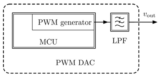
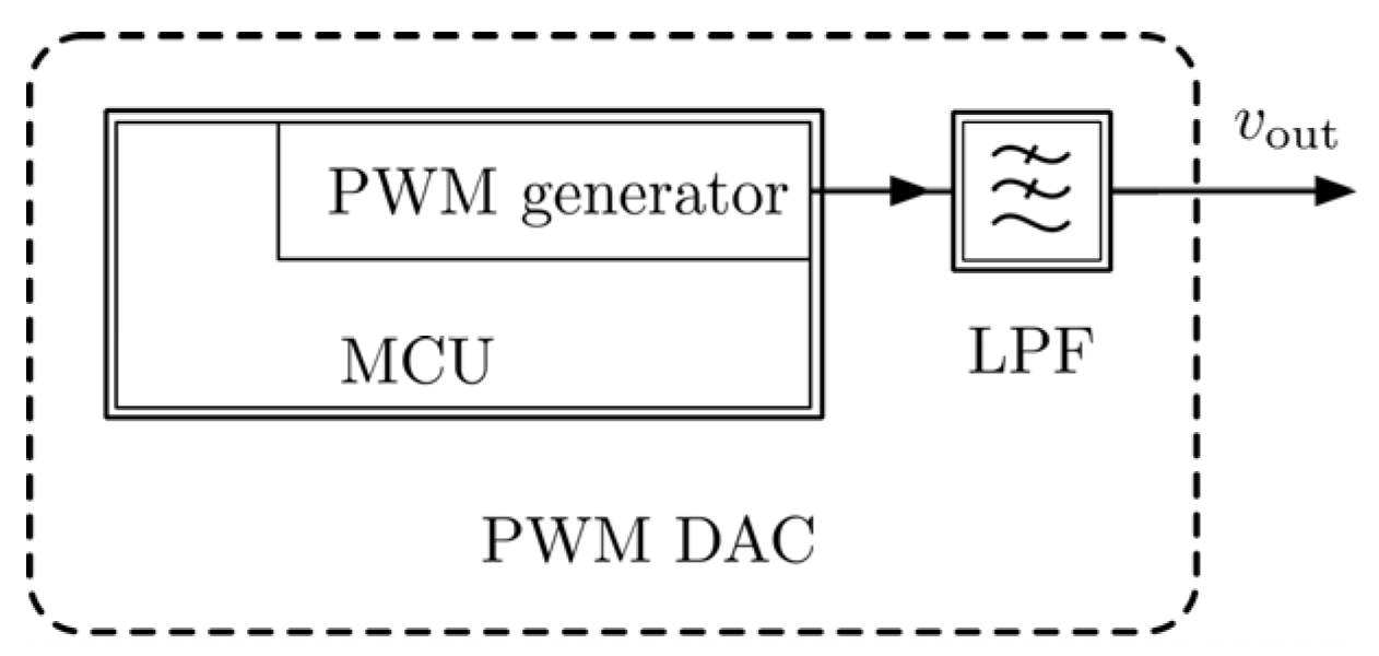
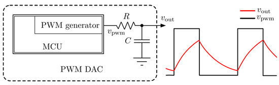
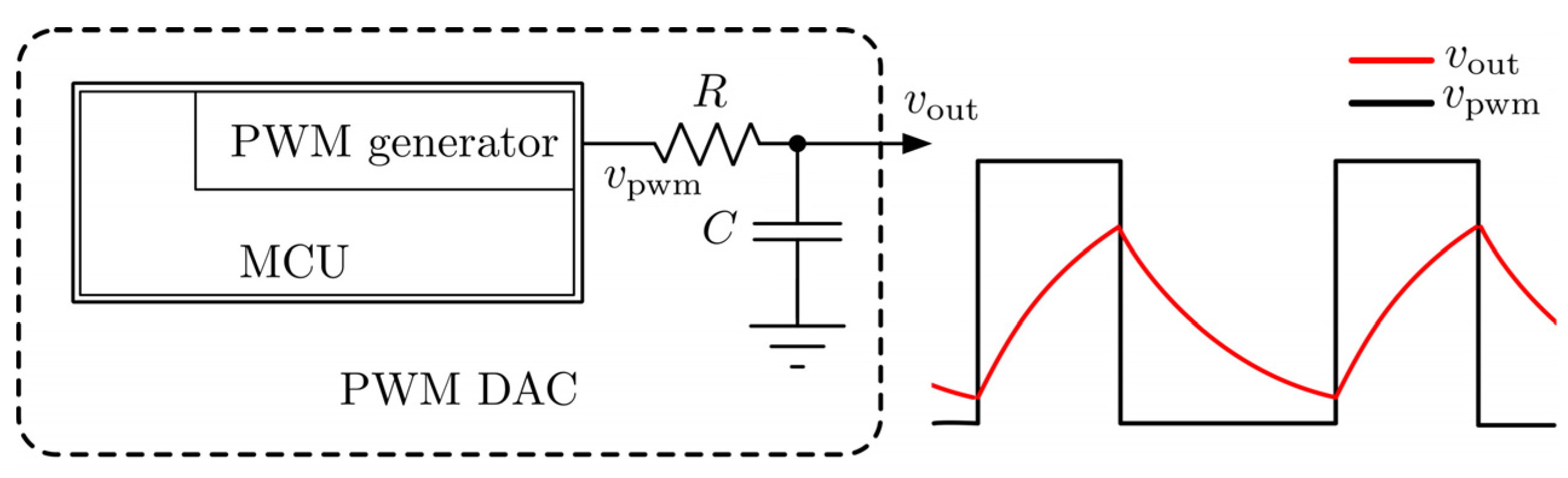
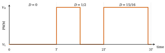
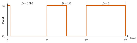
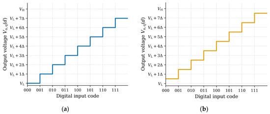
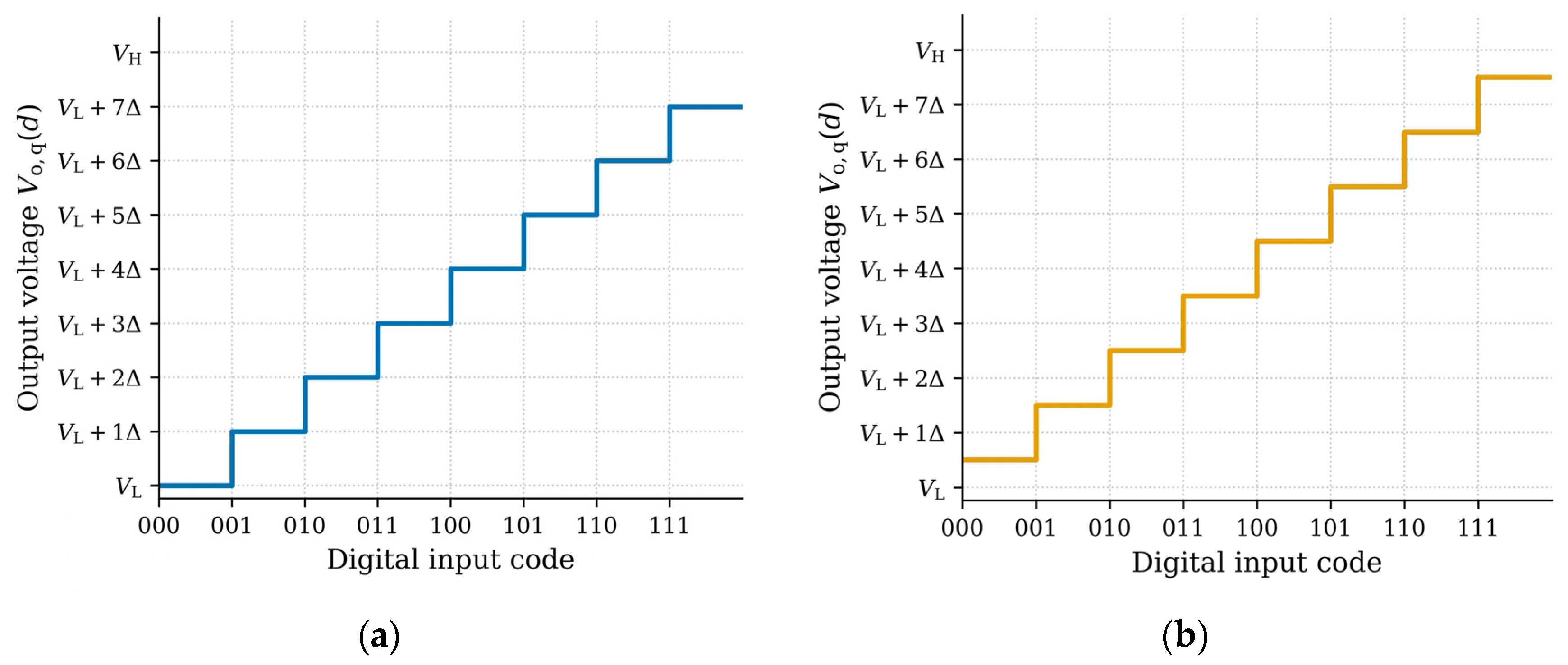
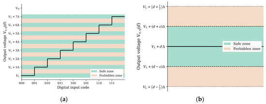
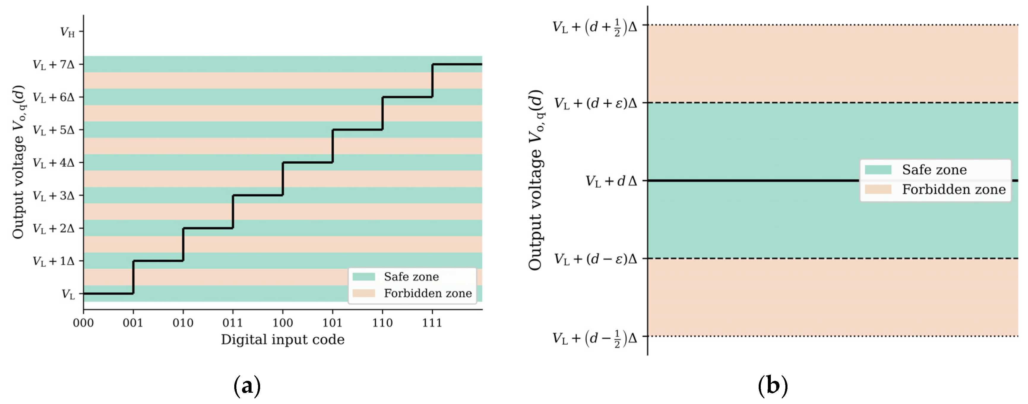
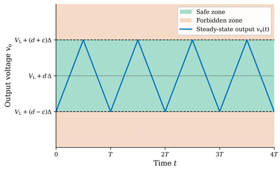
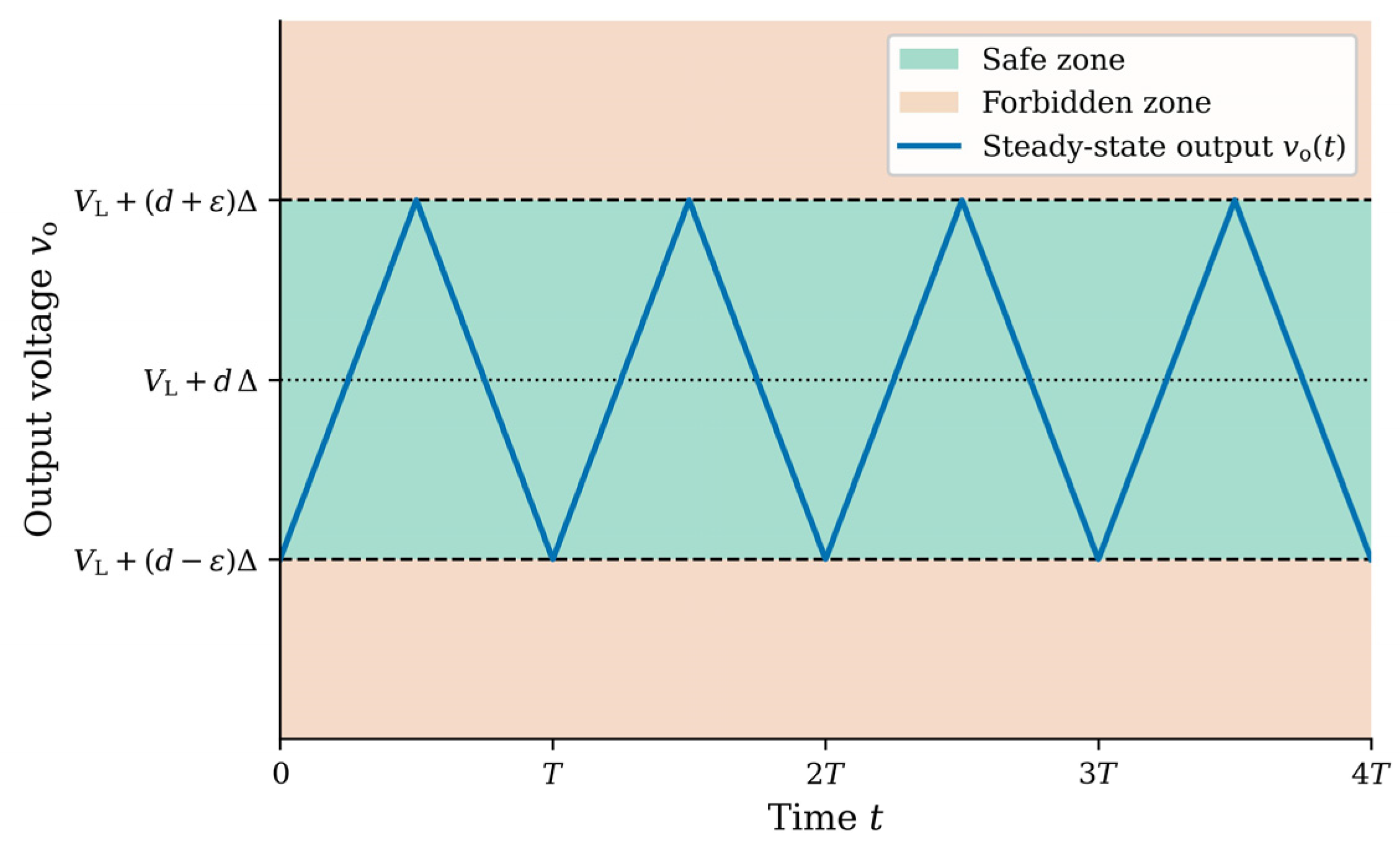
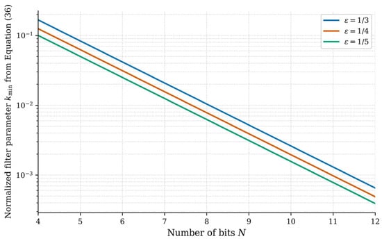
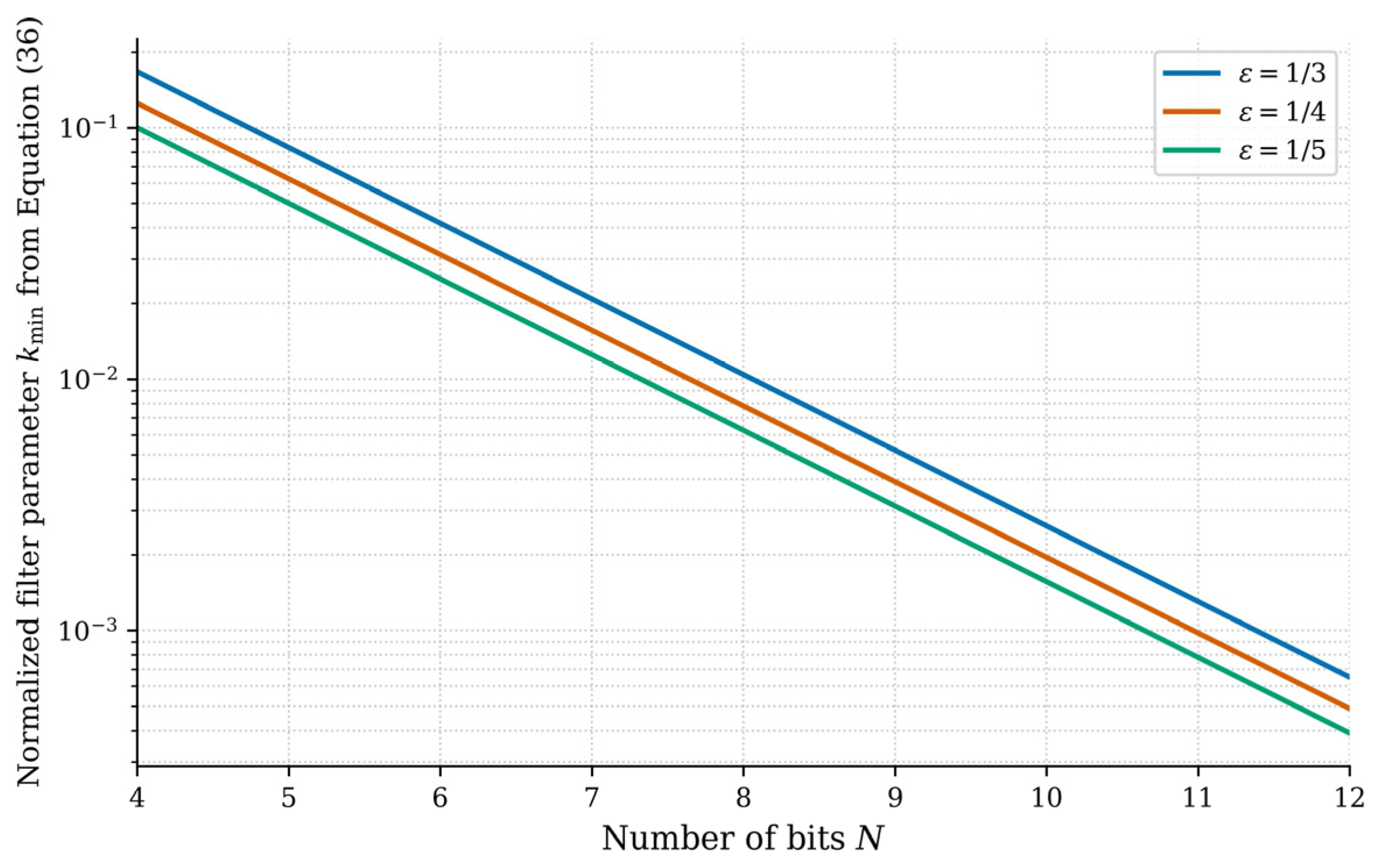
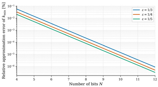
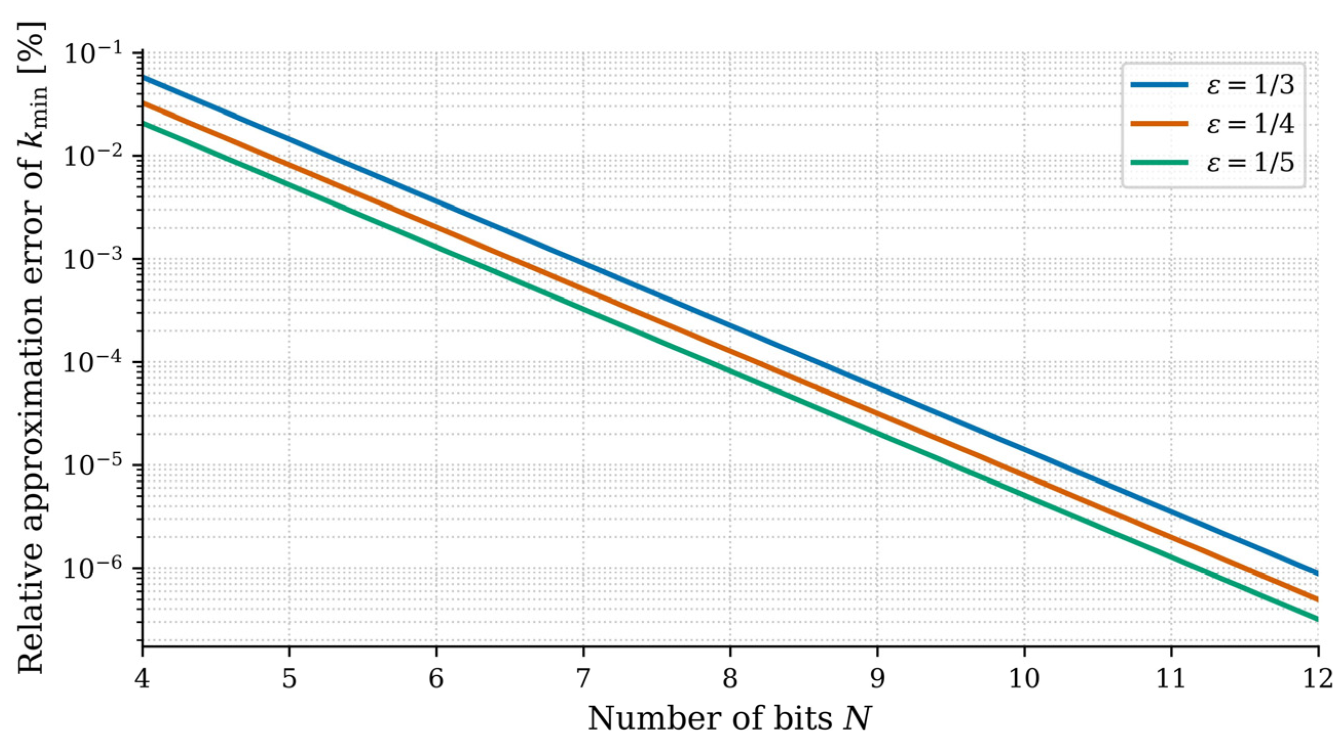
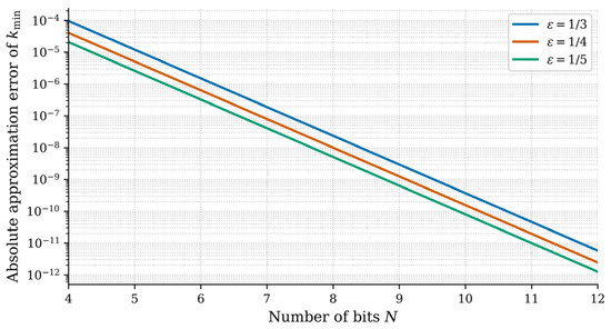
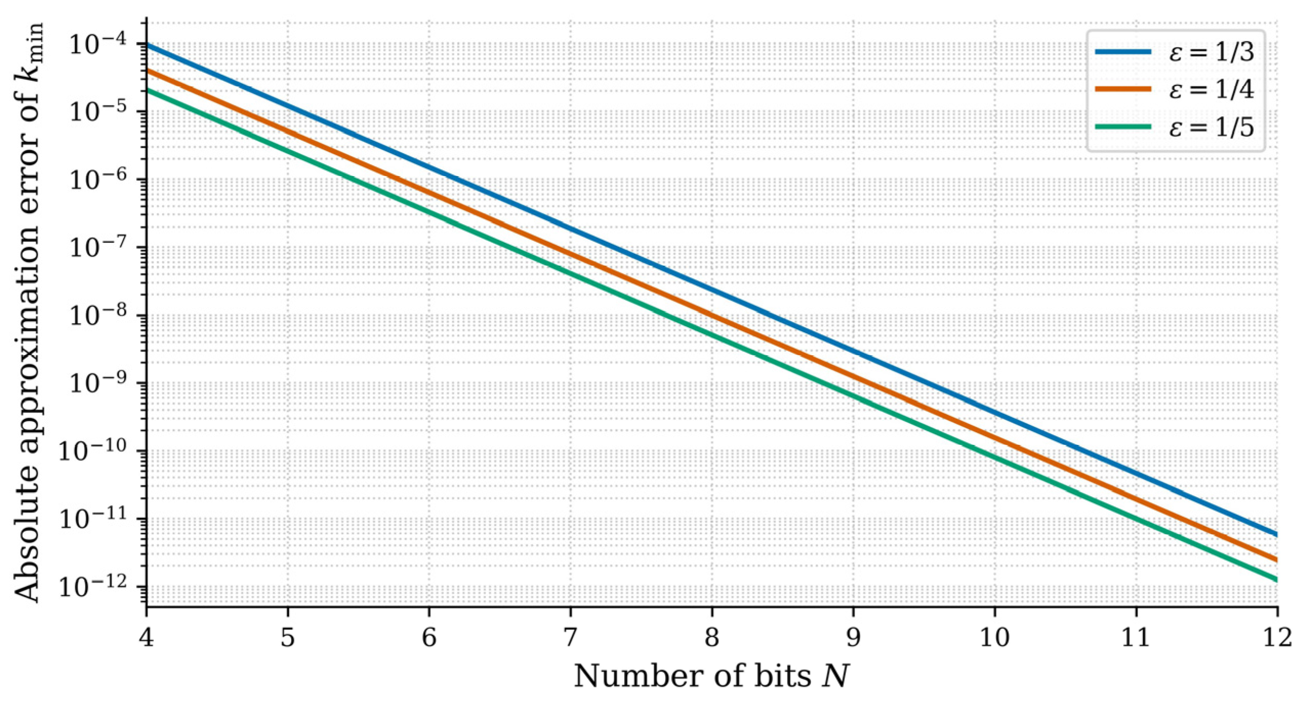
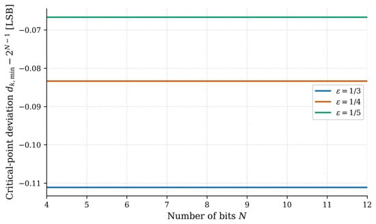
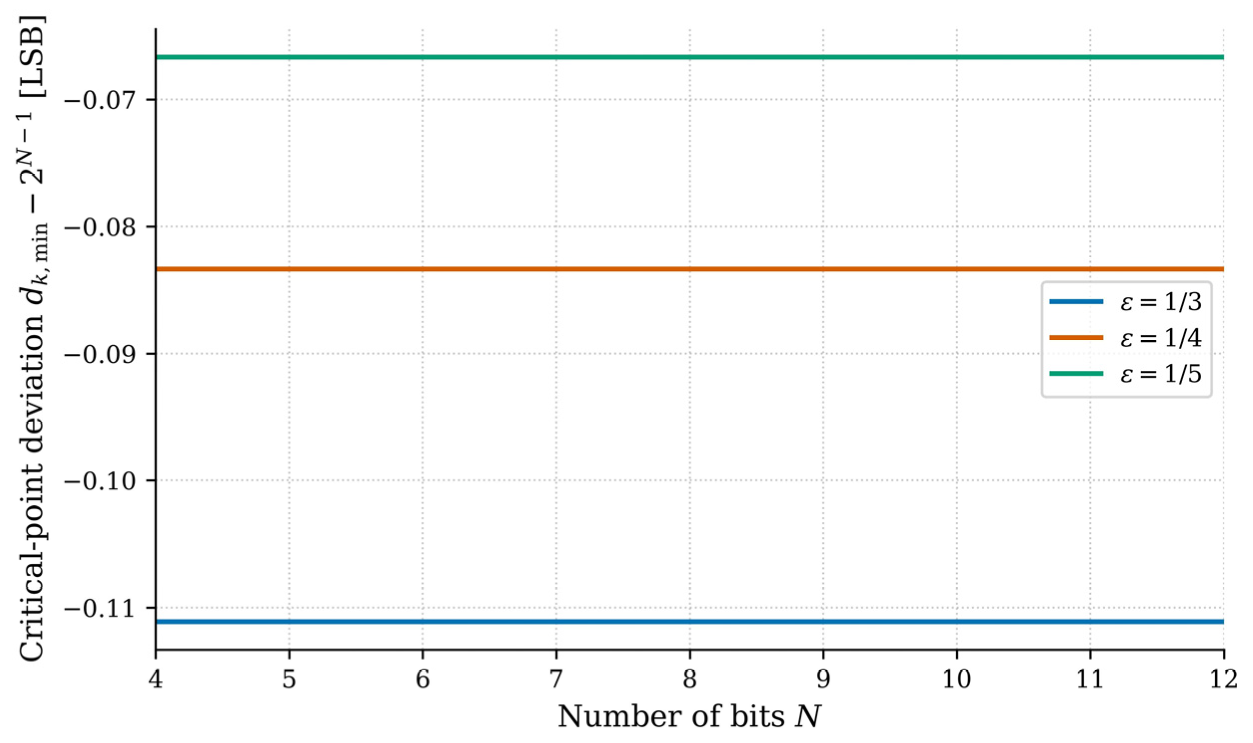
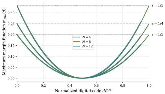
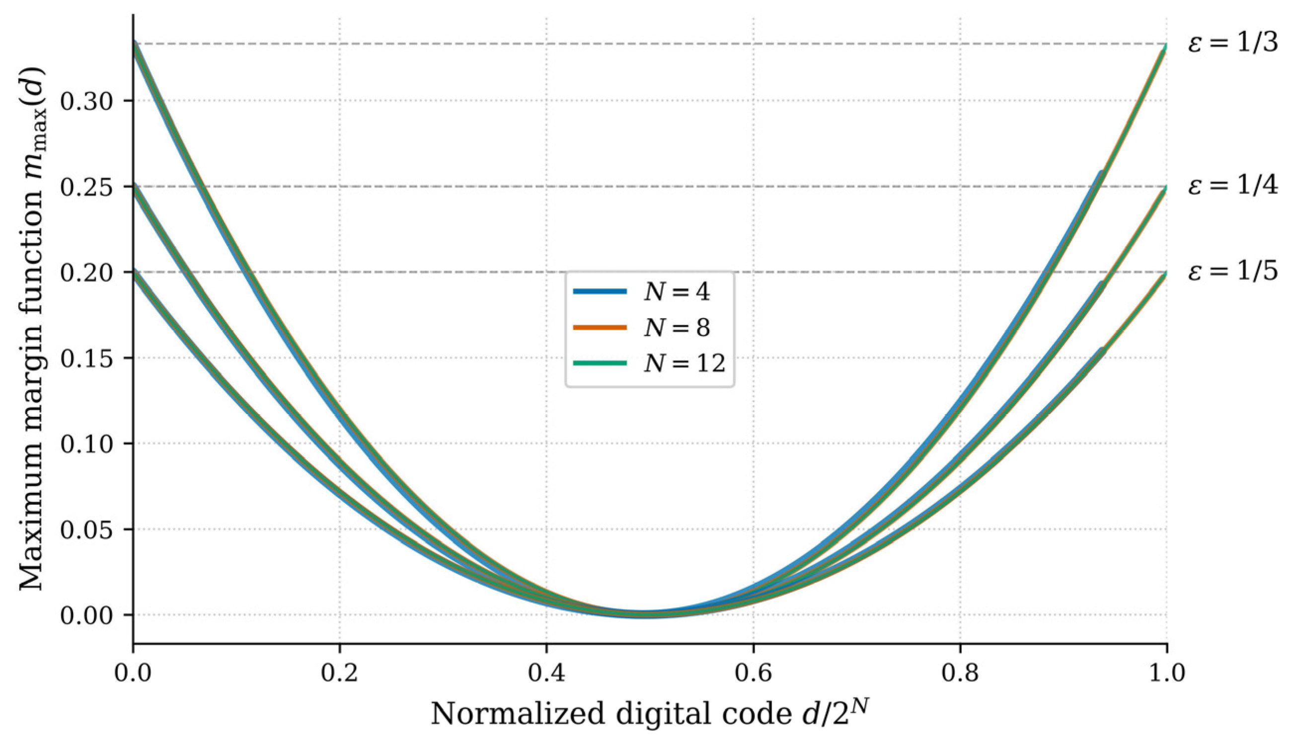
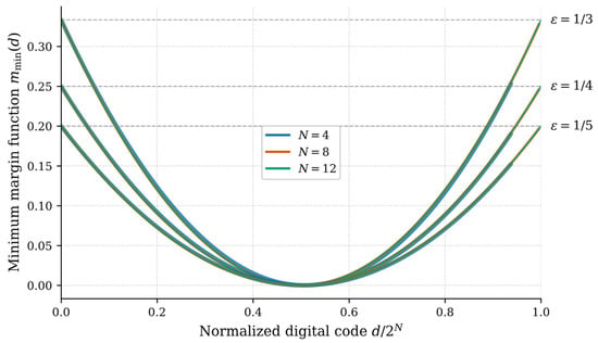
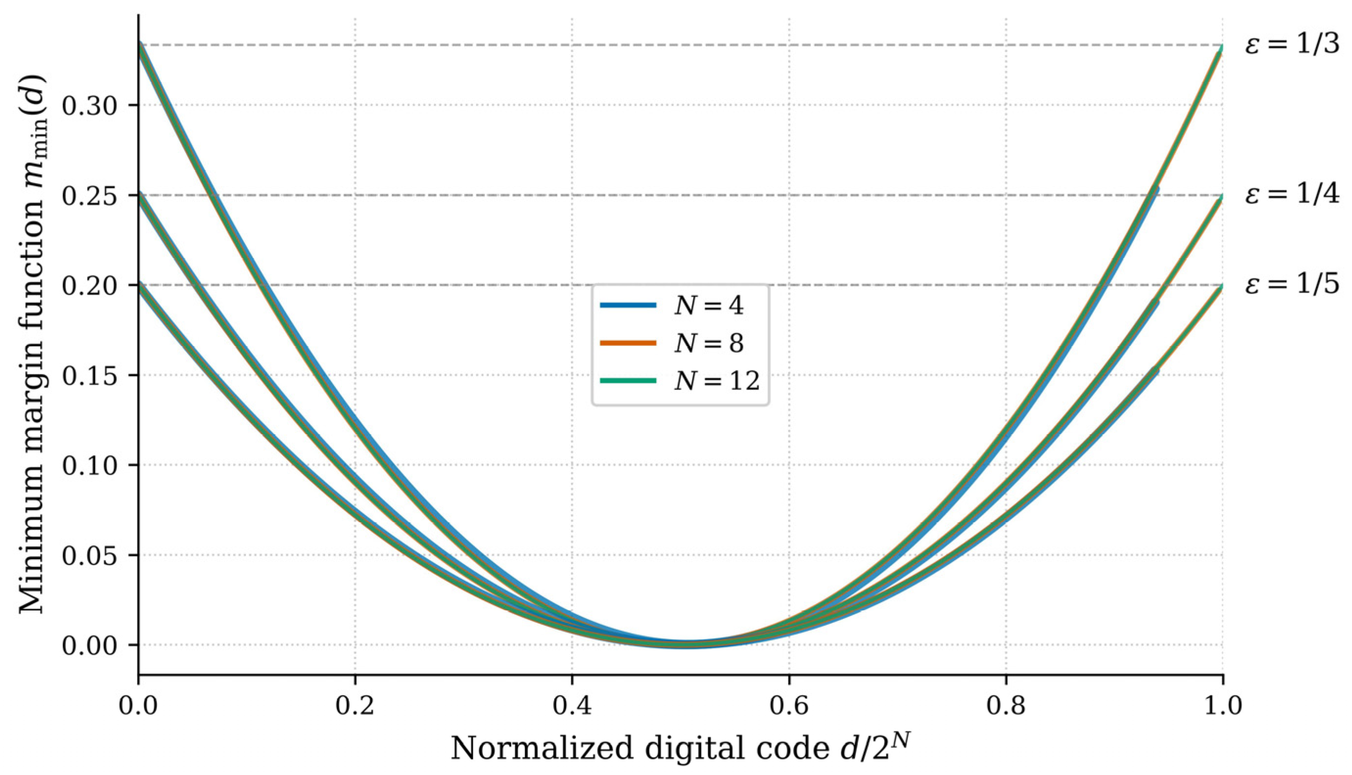
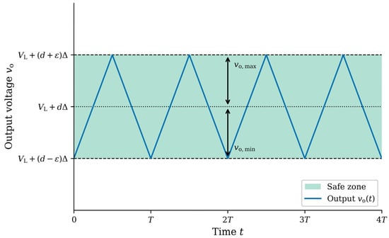
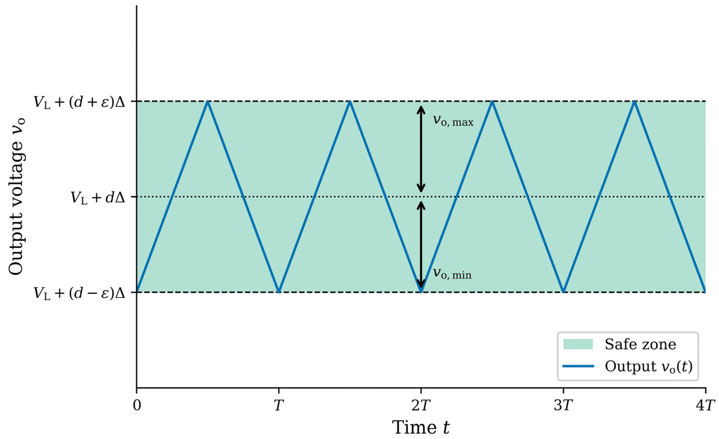
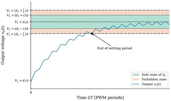
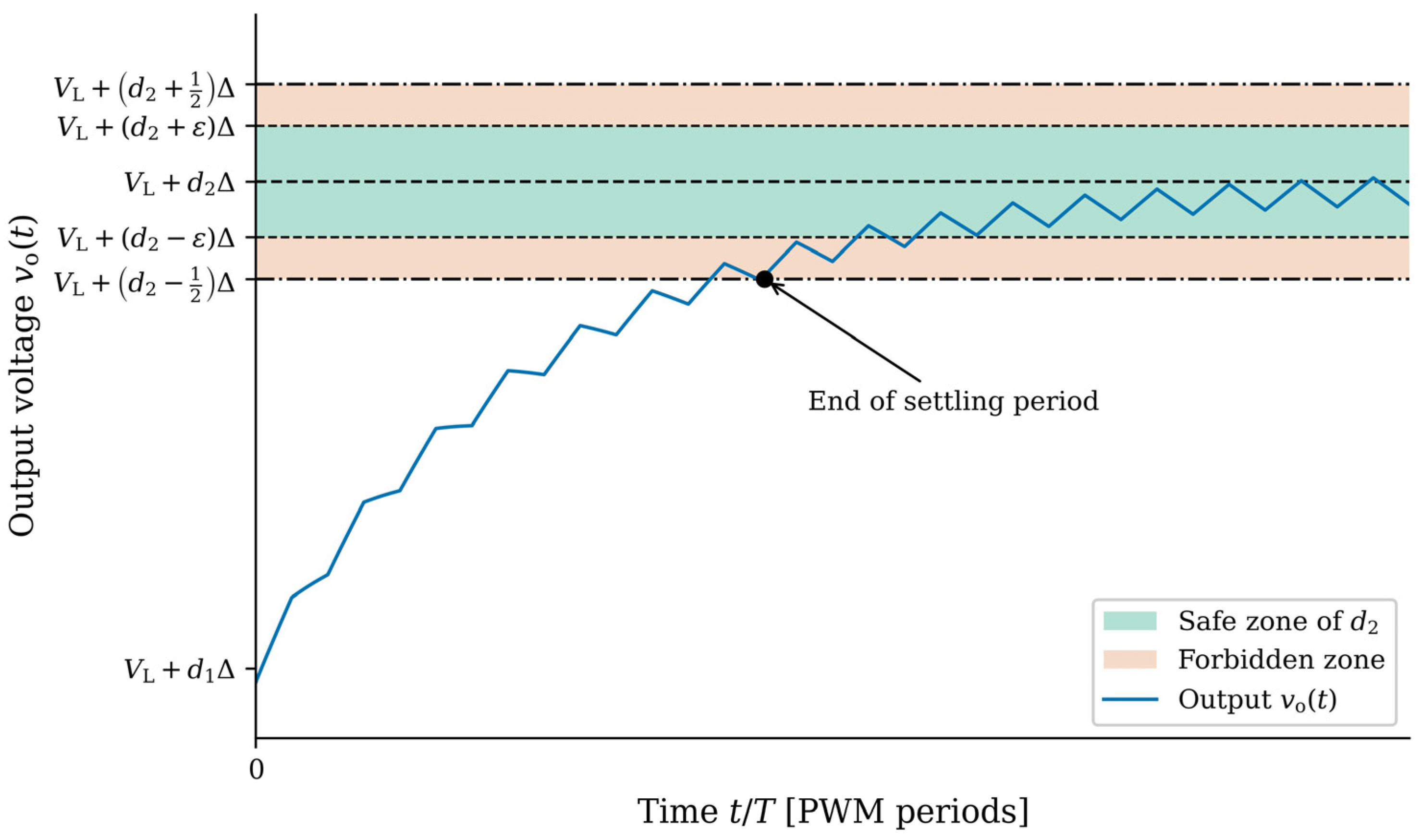
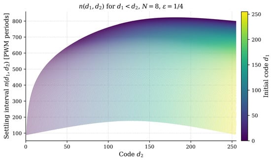
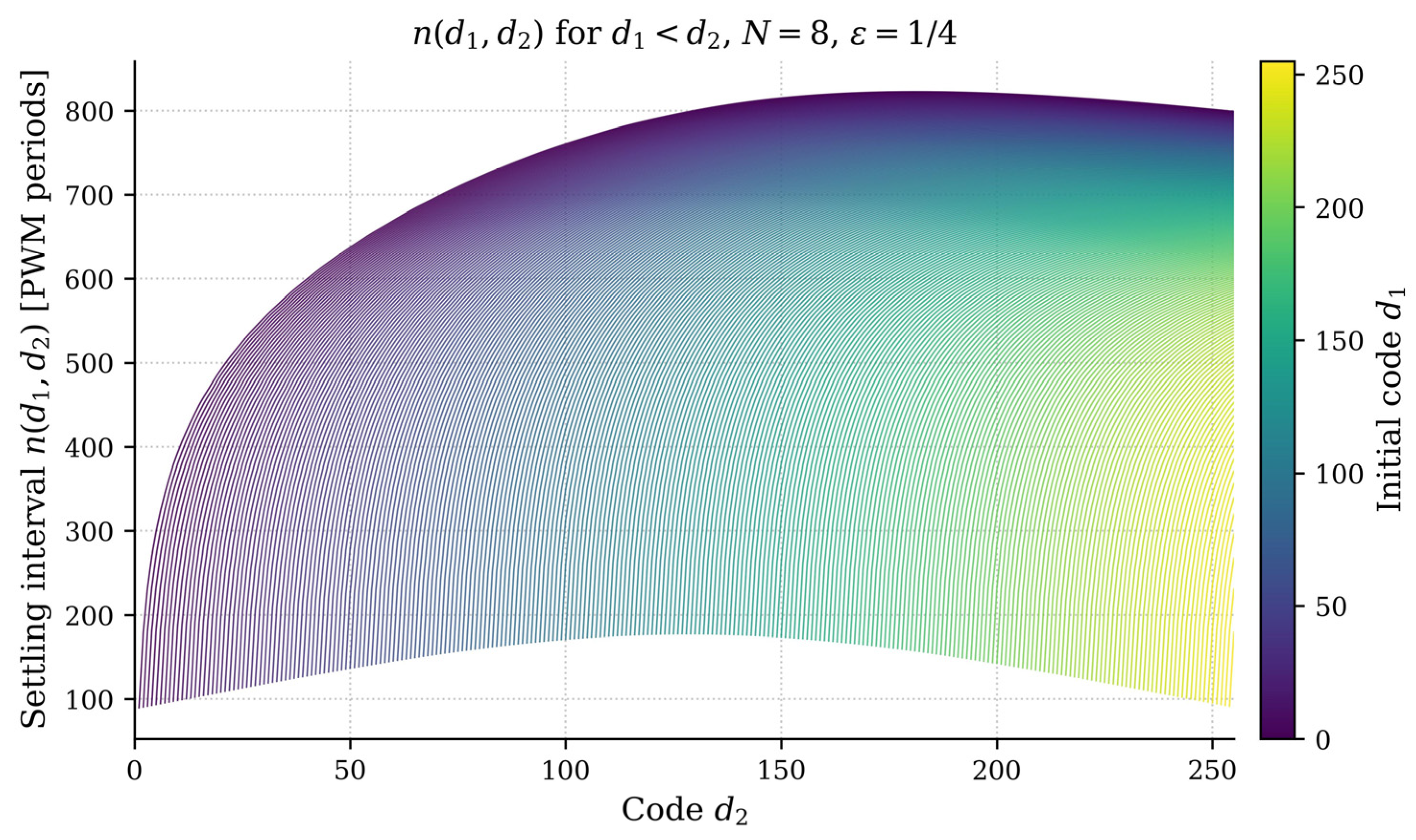
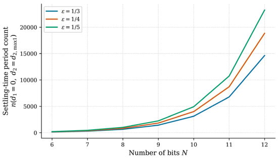
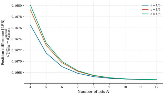
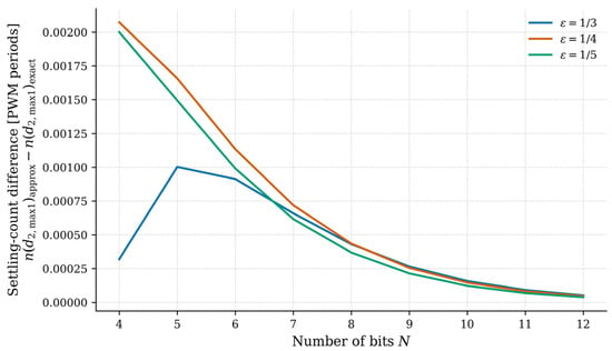
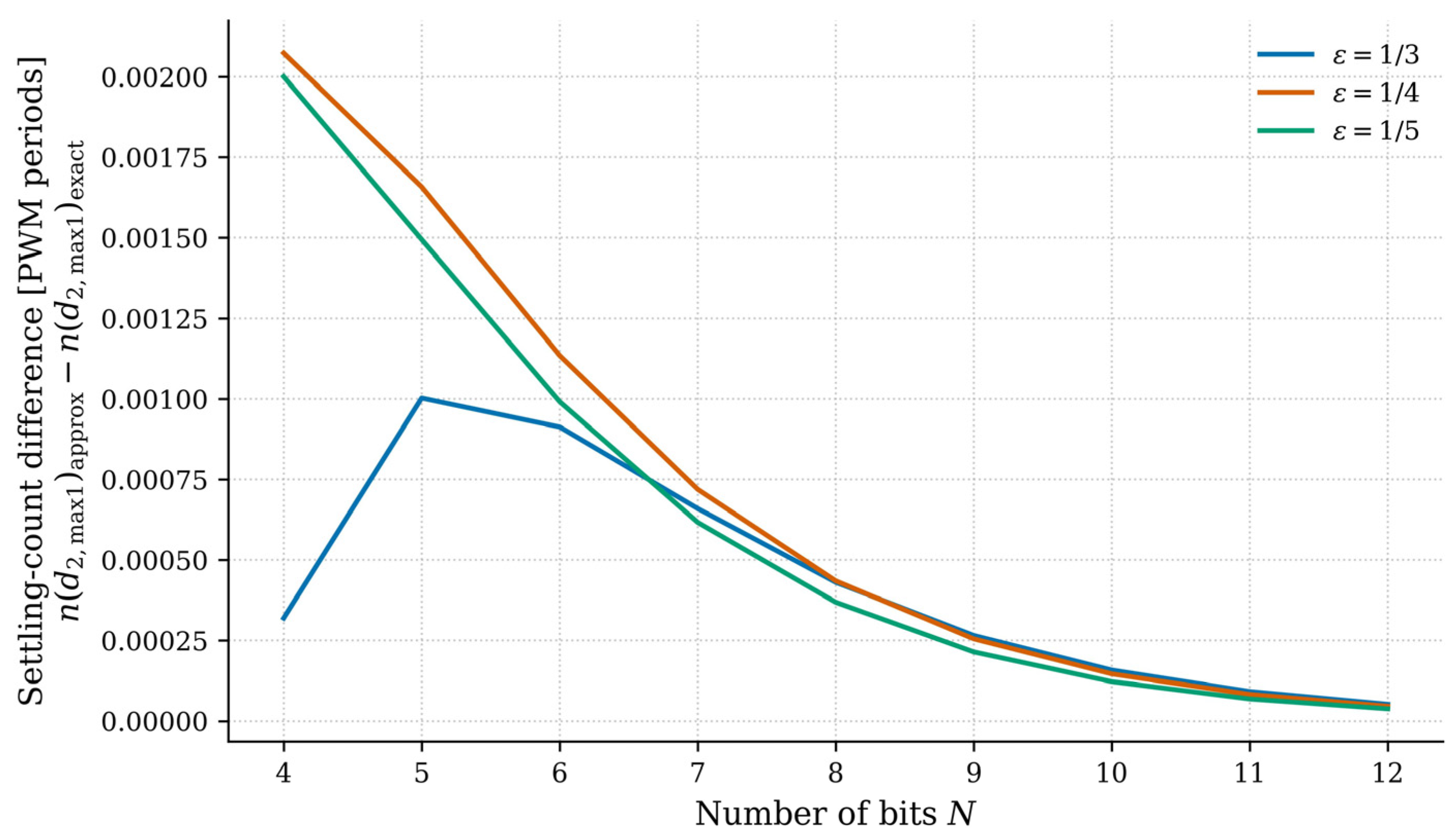
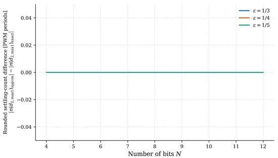
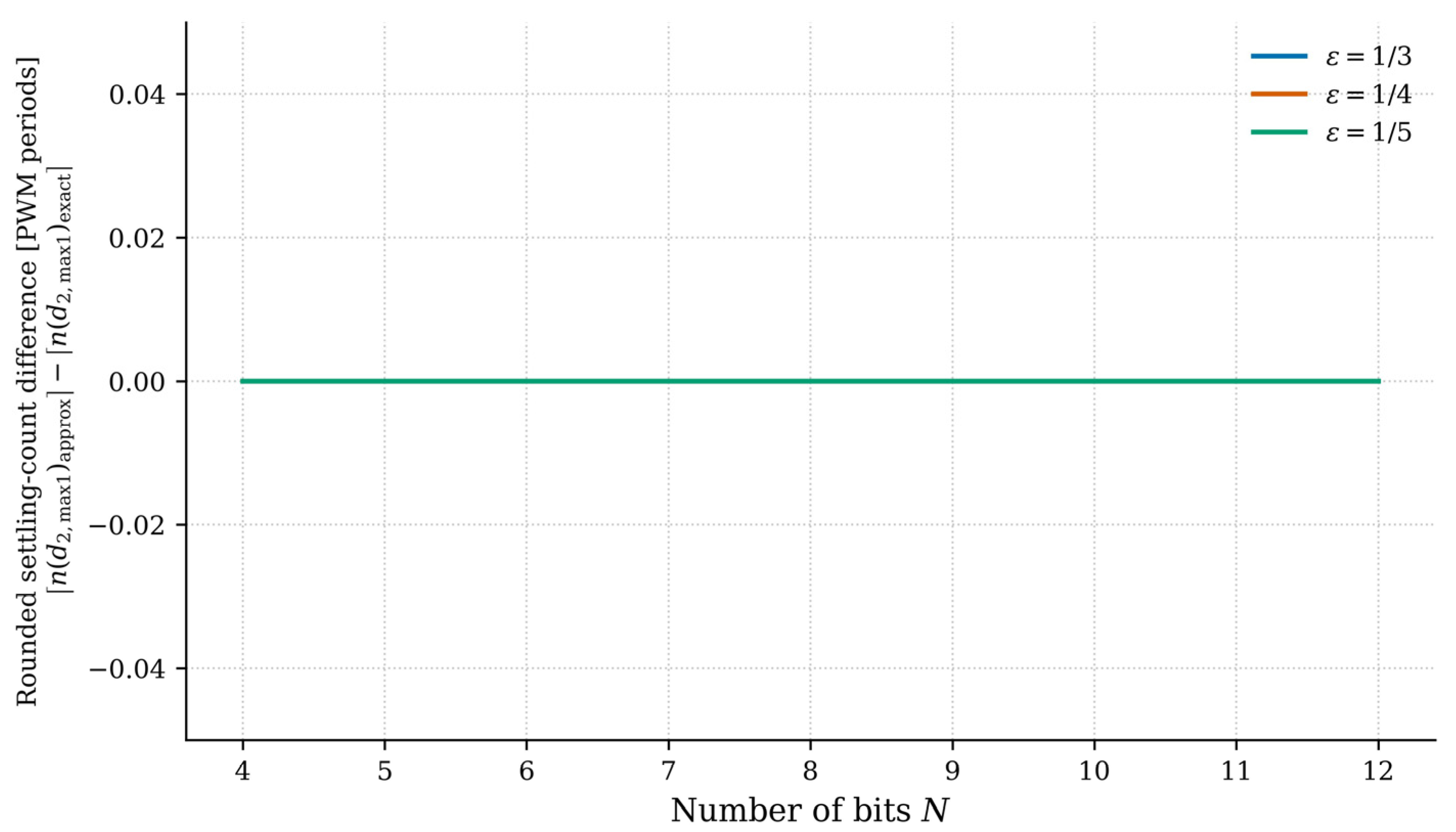
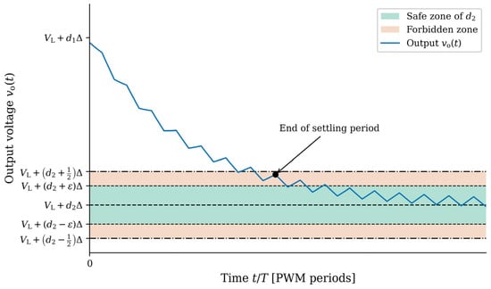
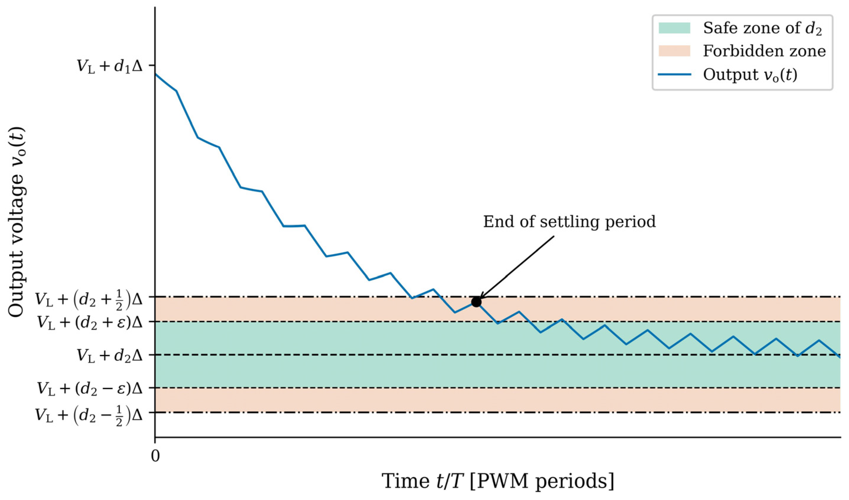
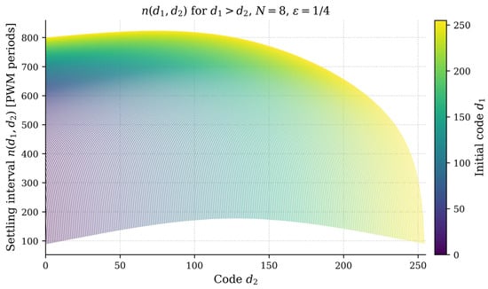
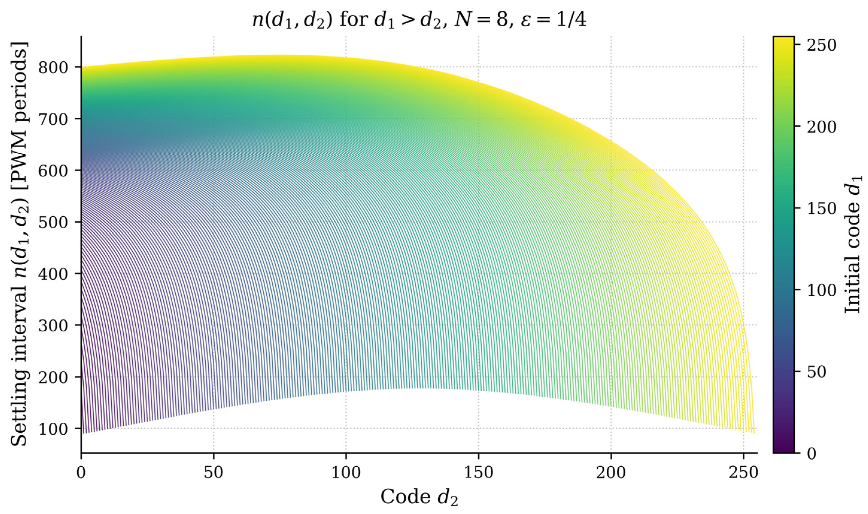
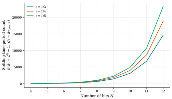
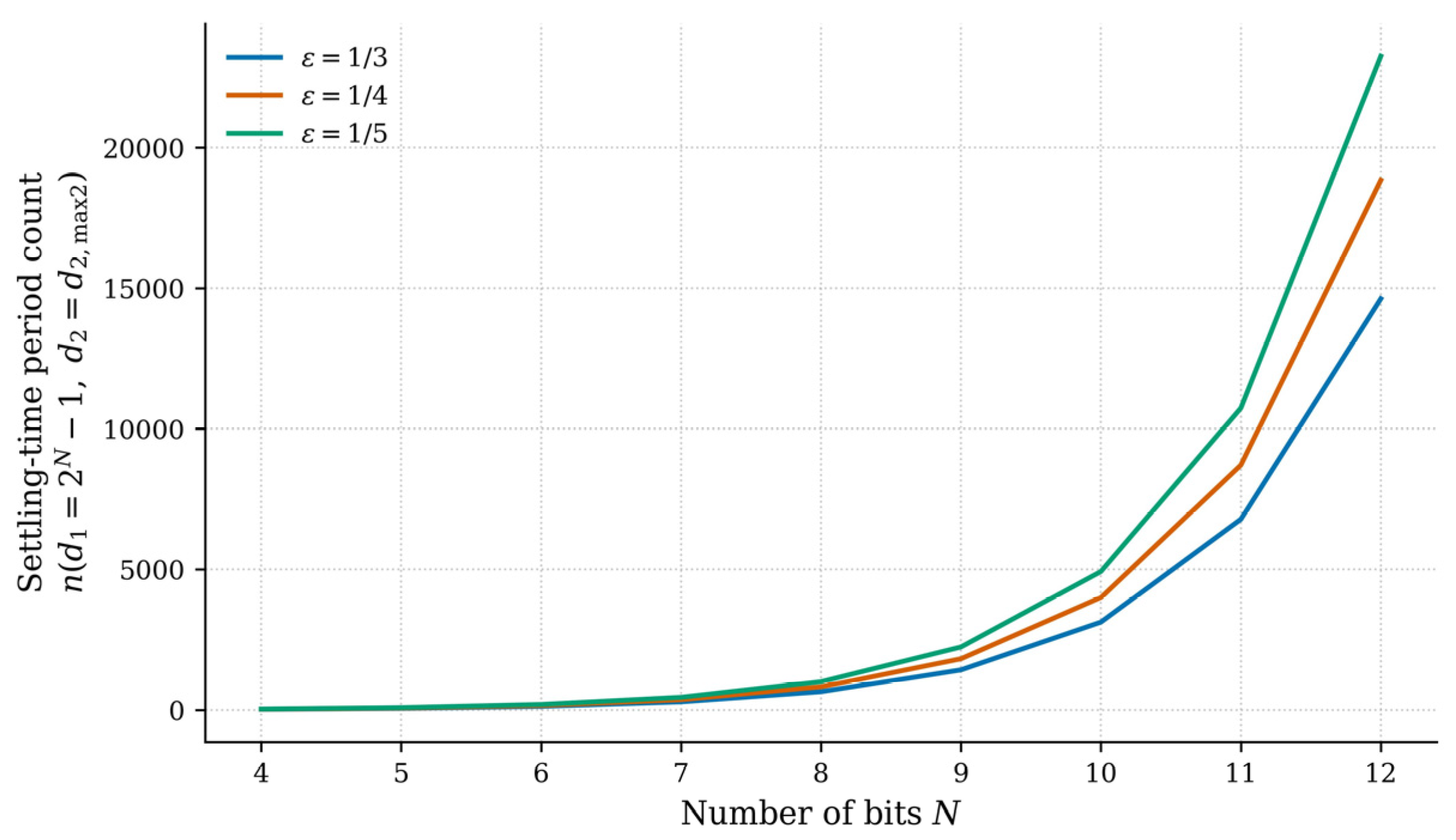
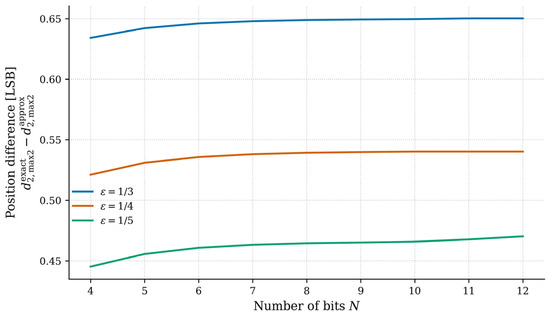
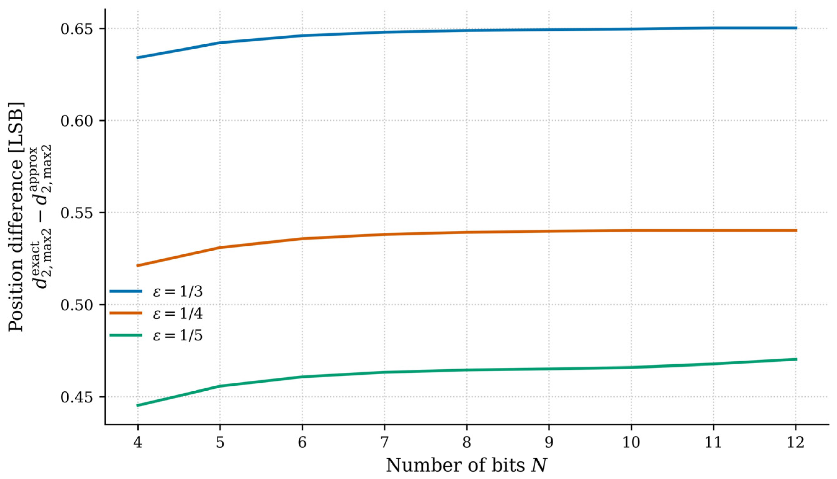
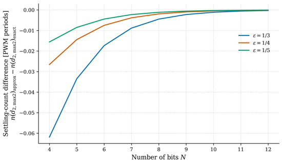
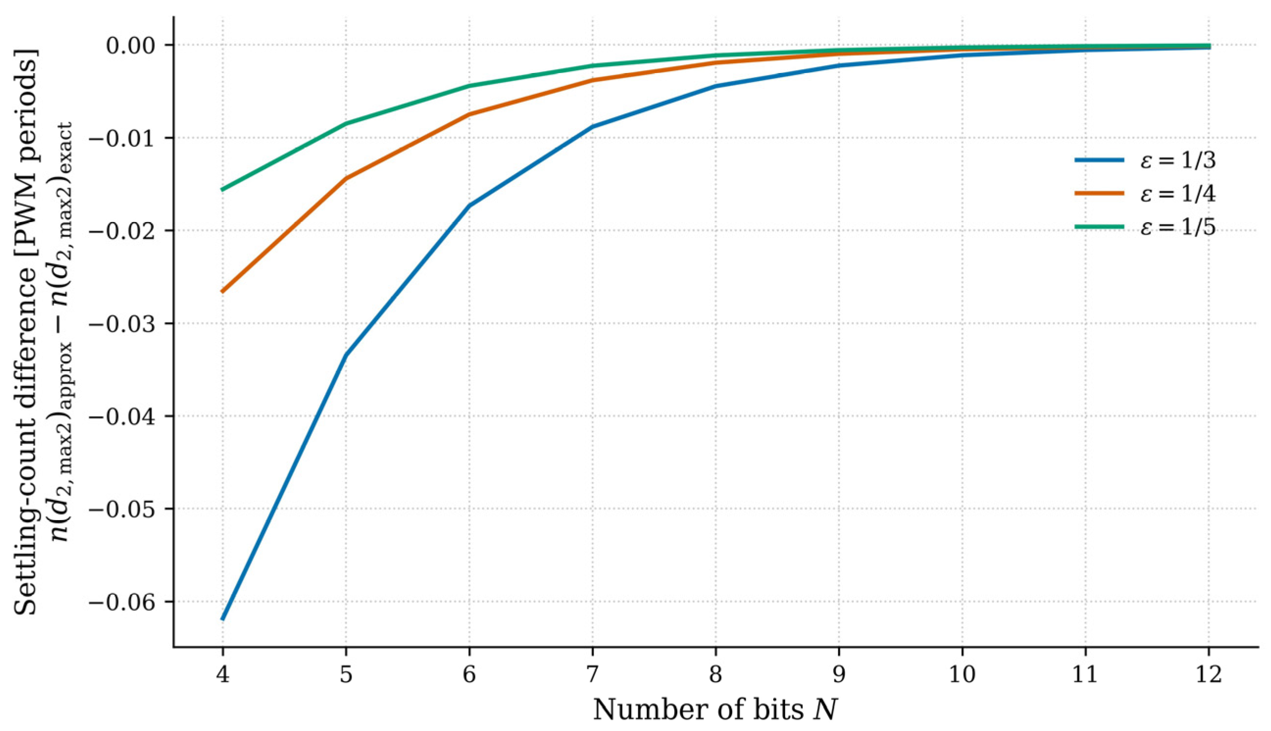
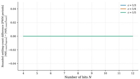
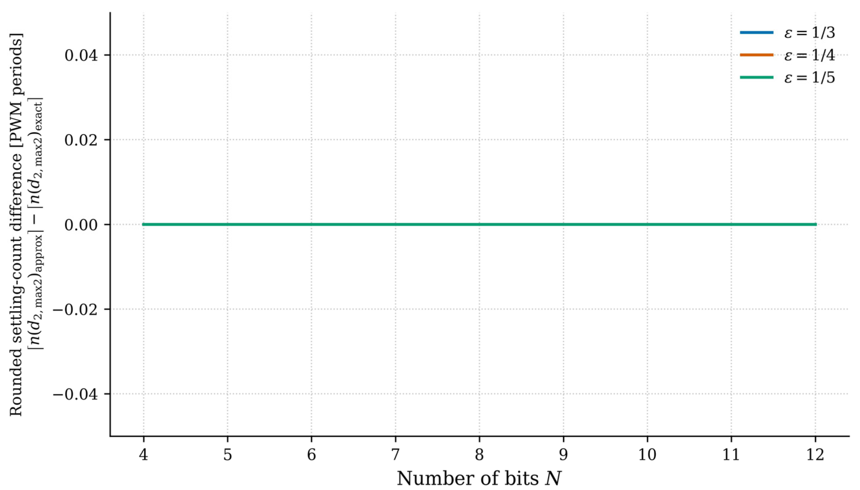
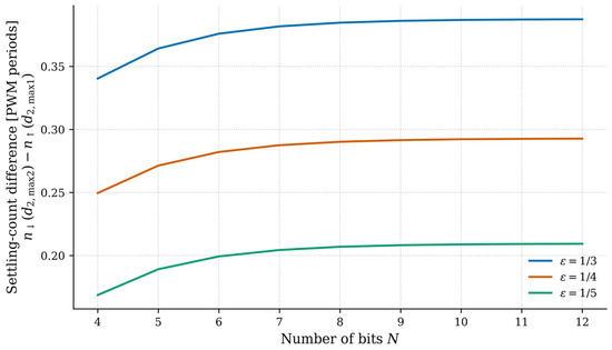
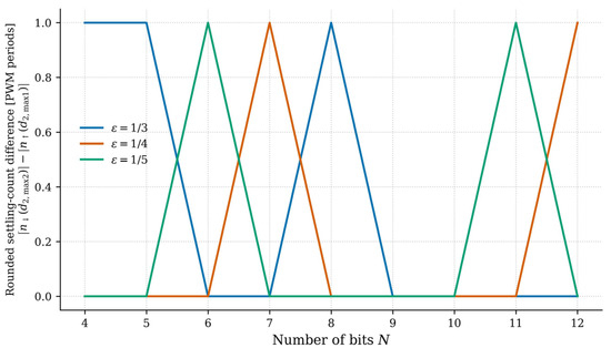
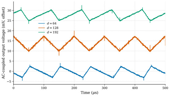
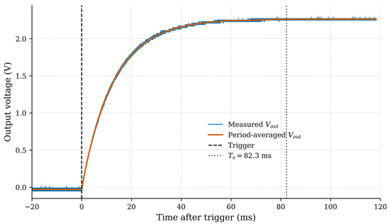
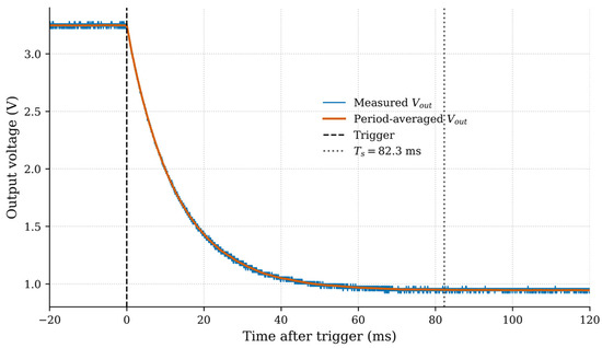
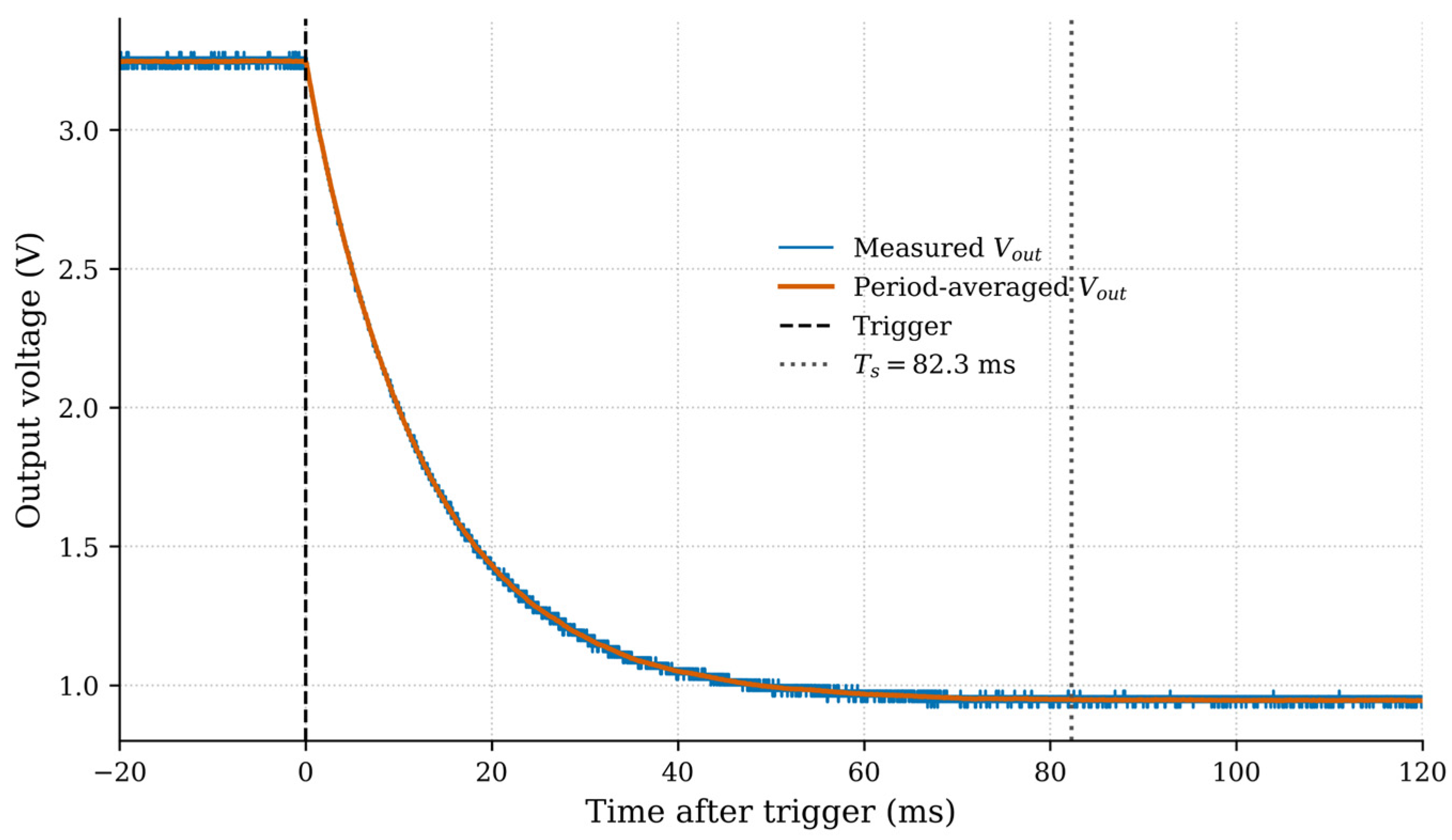

Disclaimer/Publisher’s Note: The statements, opinions and data contained in all publications are solely those of the individual author(s) and contributor(s) and not of MDPI and/or the editor(s). MDPI and/or the editor(s) disclaim responsibility for any injury to people or property resulting from any ideas, methods, instructions or products referred to in the content. |
© 2026 by the authors. Licensee MDPI, Basel, Switzerland. This article is an open access article distributed under the terms and conditions of the Creative Commons Attribution (CC BY) license.