A Novel Enhanced Binary Classification Approach Based on Hybrid GWO-PSO Algorithms for Fault Detection in Smart Grids

Abstract

Due to the complexity of recent power grids, any fault can dramatically affect the system’s quality, reliability, and stability. As a result, identifying faults becomes essential to maintaining the stability and reliability of power systems within acceptable thresholds. This article presents an innovative binary classification fault detection method in recent power grids. The proposed methodology primarily consists of two preliminary stages before the training phase: data preparation and pre-training, aimed at improving the performance of the classifier. During the data preparation phase, the synthetic minority over-sampling approach balances the raw data, and the pre-training phase identifies the optimal features and hyperparameters. A novel hybrid approach combines the Grey Wolf Optimization (GWO) and Particle Swarm Optimization (PSO) methods to optimize feature selection and adjust hyperparameters. Furthermore, four machine learning models are trained and evaluated using an actual fault dataset. In addition, several evaluation criteria and receiver operating characteristic curves are used to validate the strength and robustness of the suggested method. All experimental evaluations were performed in an Azure Machine Learning Studio (AMLS) environment. The experimental results are compared to previous studies to verify the superiority of the suggested technique.

1. Introduction

Electrical power systems are among the most critical infrastructures in modern societies. Maintaining an acceptable level of power quality, reliability, and operational stability is therefore a fundamental responsibility of utility providers. Despite continuous efforts to improve system protection and monitoring, faults in power systems cannot be completely avoided. For this reason, the development of fast and accurate fault detection methods remains essential for reducing system disturbances and limiting their consequences [1]. In general, fault detection in power systems relies on the analysis of voltage and current signals [1]. However, the distinction between normal and faulty operating conditions is not always clear, which makes the extraction of meaningful fault-related information a challenging task. Consequently, feature extraction and data representation techniques play a vital role in improving the ability of detection systems to identify abnormal conditions [2]. Existing studies have employed different feature extraction approaches, including signal transformation methods and dimensionality reduction techniques [3,4,5,6,7].

Several fault detection and classification methods have been reported in the literature. Earlier studies investigated the use of artificial neural networks, support vector machines, wavelet-based techniques, fuzzy logic, and neuro-fuzzy models for identifying faults in power systems [8]. The work [5] introduced a fault-finding approach that utilizes Artificial Neural Network (ANN) and Support Vector Machine (SVM). This method makes use of data obtained from substations and relay switchgear. Jamil et al. introduced an ANN-based method for detecting and classifying faults in transmission lines. The methodology was developed using a simulated dataset [9]. The study [7] proposes a technique that combines the Back-Propagation Neural Network (BPNN) with the Discrete Wavelet Transform (DWT) and Clarke transformation to detect faults in energy transmission lines.

Previous research studies have presented several strategies for fault detection, location, and classification. These techniques utilize fuzzy logic [10], neuro-fuzzy [11], adaptive neuro-fuzzy [12], and adaptive wavelet neuro-fuzzy [13]. A hybrid wavelet and adaptive neuro-fuzzy method were proposed to determine the faulty signals on series compensated energy transmission lines [12]. Fault detection using simulated data and based on three classifiers, Probabilistic Neural Network (PNN), Adaptive Network Fuzzy Inference System (ANFIS), and Generalized Regression Neural Network (GRNN) were introduced in [14]. Fault detection in energy transmission lines employing Concurrent Fuzzy-Logic (CFL) and using simulated data was presented in [15,16].

Ensuring a balanced distribution of data sets is crucial for improving the performance of classifiers [17]. A hybrid classification method that combines the Long Short-Term Memory Network (LSTMN) and DWT to identify insulated overhead conductor faults using partial discharge was proposed in [18]. Further, balancing the dataset via SMOTE was applied.

If a classifier is capable of accurately distinguishing between normal and faulty signals, the need for additional fault detection mechanisms can be significantly reduced. In general, fault analysis techniques can be categorized into classification-based and anomaly-based approaches. The classification-based approach directly assigns the input signal to predefined classes, typically distinguishing between faulty and non-faulty conditions. In contrast, the anomaly-based approach models the normal operating behavior of the system and identifies faults as deviations from this normal state. Therefore, any significant variation from the learned normal pattern is considered an indication of a fault [19,20,21].

Feature extraction is also an essential process that enhances the effectiveness of the classifier by extracting relevant information and minimizing the impact of variation in the dataset [2,7,9]. The Wavelet Transform (WT) is a commonly used approach for extracting features in fault diagnostic systems. In practice, most studies tend to use the DWT instead of the Continuous Wavelet Transform (CWT) to decompose the original voltage and current signals. A detailed exposition on feature selection may be available in [2].

With the rapid expansion of smart grids in terms of scale, complexity, and operational variability, traditional fault detection methods have become increasingly insufficient in handling modern system requirements [22,23]. These classical approaches often struggle to cope with the uncertainties and nonlinear characteristics associated with fault conditions in real power systems. As a result, machine learning-based techniques have emerged as powerful alternatives, offering improved accuracy, adaptability, and robustness in fault detection tasks. In particular, these methods are less sensitive to variations in system parameters and can effectively learn complex patterns from data.

Motivated by these challenges, this article proposes an enhanced fault detection framework, and its main contributions are summarized as follows:

• A data-driven fault detection framework for smart grids is developed using a real-world dataset, overcoming the limitations of simulation-based studies and enabling more practical and reliable evaluation.
• A unified two-stage optimization strategy is proposed, integrating preprocessing and pre-training phases through the novel HGWOPSO algorithm to enhance feature quality and improve model performance.
• A novel hybrid optimization algorithm, HGWOPSO, is proposed by combining GWO and PSO to achieve efficient feature selection and hyperparameter tuning while avoiding local optima.
• Extensive experiments using four machine learning models, along with thorough validation, demonstrate the effectiveness, robustness, and superiority of the proposed approach compared to existing methods.

The remainder of this article is organized as follows: Section 2 presents a general description of the fault detection system. Section 3 describes the real fault detection dataset used in this study. Section 4 discusses the optimization methods employed for feature selection and hyperparameter tuning. Section 5 explains the proposed methodology and the utilized machine learning models. Section 7 presents the obtained results and comparative analysis. Finally, Section 8 concludes the article.

2. Characterization of Fault Detection System

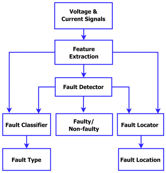
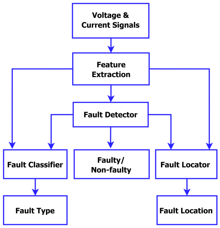
Figure 1 illustrates the fault detection general mechanism. Initially, the voltage and current signals that have been sampled are sent to the feature extraction subblock. The main task of the feature extraction subblock is to identify the relevant features and transmit them to the fault detection subblock. The task of the fault detector is to decide if the sampled signal contains fault or not. Next, the extracted features and the determination of the fault detector are concurrently transferred to the fault locator and classifier subblocks. The fault classifier differentiates between different fault types, whereas the fault location identifies the specific fault zone.

Figure 1. Fault detection mechanism model.

3. Real VSB-ENET Dataset

This article employs the real fault detection dataset developed at the Technical University of Ostrava (VSB) by the Energy and Environmental Technology Laboratory (ENET) [24]. The ENET center collects the fault data of energy power lines with smart meters at 20 ms. The measurements at all phases were registered synchronously. The dataset contains 8712 signals, each including 800 k samples of the line voltage measurements. The first time using this dataset was in 2018 when a competition announced on the Kaggle website to discover the partial discharge patterns within the collected signals. The dataset was available as “Apache Parquet” files on the Kaggle website, which were converted into “CSV” files to perform this study. Each signal has 19 input features and one output, either ‘0’ or ‘1’. A value of ‘1’ symbolizes the faulty state, while ‘0’ symbolizes the normal state. Moreover, the VSB-ENET dataset is an imbalanced dataset comprising 94% normal or non-faulty and 6% faulty singles.

4. Methods of Optimization

The Grey Wolf Optimization (GWO) and Particle Swarm Optimization (PSO) algorithms can achieve successful results in almost optimization problems [25,26]. In this artilce, the hybrid (HGWOPSO) algorithm that combines the GWO [27,28,29] and PSO [30,31,32] optimization methods is utilized. The following sections describe in detail the HGWOPSO method.

4.1. Grey Wolf Optimization

The GWO algorithm simulates the hunting behavior of grey wolves in their natural environment. It primarily consists of three phases of hunting: locating the prey, surrounding the prey, and then assaulting the prey, which is employed for optimization [33]. The GWO process has three primary components. Initially, all gray wolves (search agents) within the population are randomly started within the range [LB, UB]. Subsequently, the fitness score for each search agent is evaluated using the corresponding objective function. The best response thus far is alpha, succeeded by beta and delta, respectively. At this point, the remaining wolves are organized under the omega. In GWO, delta, alpha, and beta essentially do the optimization, with omega coming in second. Subsequently, search agents adjust their positions in accordance with the prey’s location as delineated by Equations (1)–(3).

$$D_{\alpha }=\mid C_1{P}_{\alpha }-P\left(t\right)\mid ,D_{\beta }=\mid C_2{P}_{\beta }-P\left(t\right)\mid ,D_{\delta }=\mid C_3{P}_{\delta }-P\left(t\right)\mid$$

(1)

$$P_{\alpha }=P_{\alpha }-A_1{D}_{\alpha },P_{\beta }=P_{\beta }-A_2{D}_{\beta },P_{\delta }=P_{\delta }-A_3{D}_{\delta }$$

(2)

$$P(t+1)={\displaystyle \frac{P_{\alpha }+P_{\beta }+P_{\delta }}{3}}$$

(3)

The notations t, $P\left(t\right)$, $P(t+1)$, $P_{\alpha }$, $P_{\beta }$, and $P_{\delta }$ stand for the current iteration, the prey’s position at that moment, the prey’s position in the subsequent iteration, and the positions of alpha, beta, and delta, successively. The vectors A and C are calculated as follows.

$$A=2a\ast r_1-a$$

(4)

$$C=2r_2$$

(5)

Here, $r_1$ and $r_2$ denote random vectors uniformly distributed throughout the interval [0, 1], whereas a represents the control vector that linearly decreases from 2 to 0 to optimize the search and exploitation of viable solutions. The GWO repeats in the identical method up to the maximum iteration limit is reached.

4.2. Particle Swarm Optimization

PSO is a computational searching technique that solves complex problems by iteratively refining a candidate solution based on a specified quality criterion. PSO models the behavior of avian or aquatic communities and was developed in 1995 [34]. A swarm is constructed of multiple particles. Each particle is regarded as a candidate solution. For every particle i, there are three vectors at the present repetition t: length N, personal best, velocity, and location. The position vector ($P_t^i$) indicates the present location of the particle in the exploring range, and the velocity vector ($V_{(t+1)}^i$) specifies the speed and direction of the particle at the subsequent iteration; meanwhile, the personal best ($P_{best}^i$) identifies the optimal placement of the explored particle.

Furthermore, the global best ($G_{best}$) is another crucial vector for the swarm, which stores the optimal placement of the analyzed swarm. At the end of every repetition, the local best vector for every particle and the global best vector for the swarm are modified. The local best vector represents the particle’s mental expertise, but the $G_{best}$ denotes the swarm’s social knowledge [35]. At the subsequent repetition $t+1$, the position and velocity vectors are calculated as follows.

$$V_{t+1}^i=W\times V_t^i+C_1\times r_1\left(t\right)\times (P_{best}^i-P_t^i)+C_2\times r_2\left(t\right)\times (G_{best}-P_t^i)$$

(6)

$$P_{t+1}^i=P_t^i+V_{t+1}^i$$

(7)

where W is the weight of the inertia factor that regulates the influence of the velocity vector in the current repetition on the following ones to keep the particle inside the boundaries of the search space. The variable W is constant and can vary from 0.4 to 0.9 [36]. $C_1$ and $C_2$ are the acceleration factors and commonly ranged in [1, 5] [36]. Simultaneously, $r_1$ and $r_2$ are distributed equally as random variables inside the interval [0, 1]. The objective of employing the constants $C_1$, $C_2$, $r_1$, and $r_2$ is to regulate cognitive and social information regarding variations in velocity. Consequently, all particles will become oriented towards the optimal resolution of the problem. Ultimately, PSO will provide the $G_{best}$ vector as the optimum solution and terminate operation upon fulfilling the termination condition. Nonetheless, PSO will forward to the next repetition and replicate the exact process.The termination condition is met when the enhancement of $G_{best}$ falls below the halting threshold ($ϵ$) or a specified number of repetitions has elapsed.

4.3. Hybrid GWO-PSO (HGWOPSO)

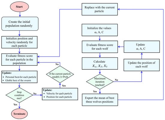
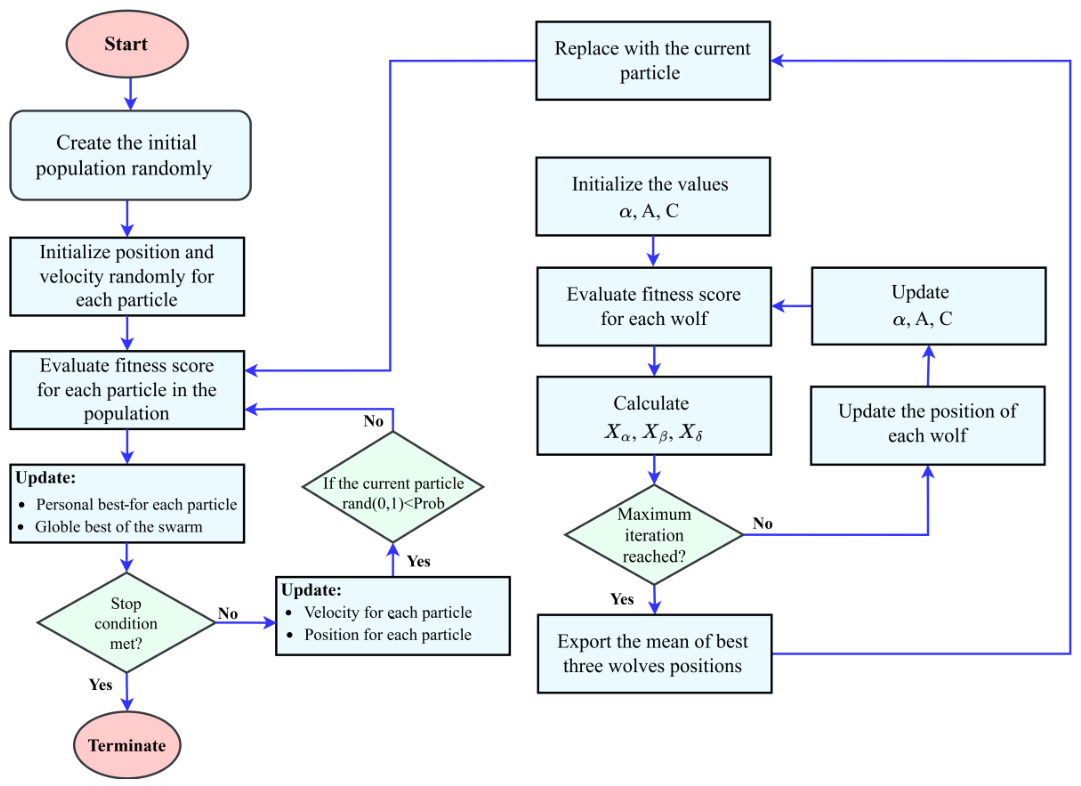
Numerous methods, such as the Satin Bowerbird Optimizer (SBO) [37], Stochastic Fractal Search-based Guided Whale Optimization Algorithm (SFS-Guided WOA) [38], Biogeography-Based Optimizer (BBO) [39], and Firefly Algorithm (FA) [40] have been suggested for picking features and hyperparameter optimization. In this paper, a novel HGWOPSO [25] is applied to optimize feature selection and hyperparameter tuning, then compared to different algorithms that appear in the literature. The PSO algorithm generally accomplishes successful results in different optimization problems; however, its main problem is that their solutions trap into a local minimum. HGWOPSO can mitigate the issue of converging to a local minimum and get effective outcomes by employing the GWO algorithm. GWO prevents the particles from approaching random positions and directing them to improved positions. The flowchart of the HGWOPSO method is as suggested in Figure 2. In the HGWOPSO framework, the two algorithms are executed sequentially in an alternating way, the optimal hyperparameters obtained from GWO are utilized to guide the PSO particles, preventing them from converging toward random positions and instead directing them toward more promising regions of the search space. This mechanism mitigates a known limitation of PSO, namely its tendency to become trapped in local minima (as discussed in our previous work published in [41]. Through this hybridization, the optimal hyperparameters of each machine learning model can be determined more accurately and robustly.

Figure 2. Flowchart of the HGWOPSO.

5. Methodology

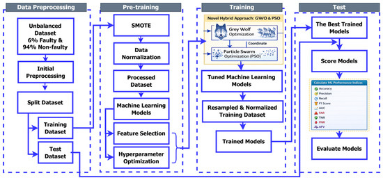
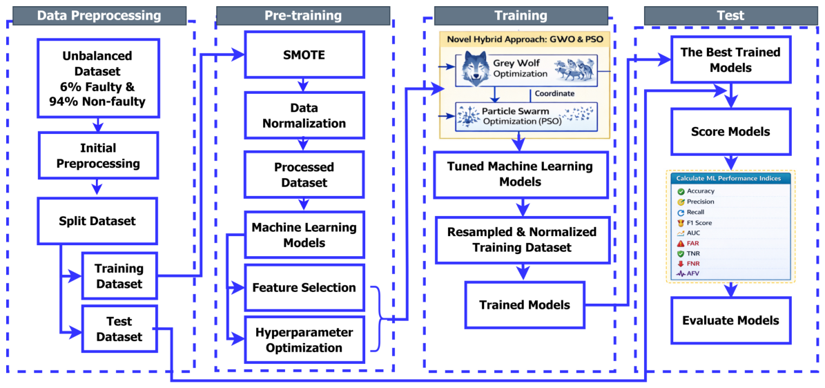
This study’s approach comprises four phases: data preparation, pre-training, training, and testing, as seen in Figure 3. In the following subsections, these phases are illustrated in detail.

Figure 3. Proposed methodology.

5.1. Data Preprocessing

During the preprocessing phase, the raw data are refined to improve the effectiveness of the classifier. Data balancing and normalization are the central core of preprocessing stage. As aforementioned in Section 3, the VSB dataset consists of 94% non-faulty and 6% faulty signals. The notable unbalancing of the VSB dataset causes poor classification as the classifiers tend to the majority state. Thus, balancing imbalanced data is an inescapable choice to enhance the performance of the classifier. Various resampling methods for balancing imbalanced data have been developed [42,43,44]. There are three main balancing methods, oversampling, undersampling, and ensemble [45,46]. Oversampling is a method to produce additional data from the minority group to overcome its lack [47]. The advantages of the oversampling method are that it does not cause information loss and gives adequate accuracy, while its principal drawback is that it causes an increase in data, leading to overfitting [48].

Undersampling is a method to decrease data from the majority group until it equates to the data of the minority group [42]. The undersampling method has many advantages in solving the storage problem and providing a balanced dataset that contains valuable information. A fundamental drawback of undersampling is the removal of critical information from the majority category, resulting in incomplete classifications [49]. Finally, the ensemble sampling method produces multiple models and then mixes them to offer enhanced results. One widely used oversampling method is SMOTE [50]. SMOTE is based on many steps to oversample the minority category: initially, it oversamples the minority group using synthetic oversampling rather than oversampling with replacement. Hence, SMOTE distinguishes the minority group samples, which are the k-nearest neighbors of the desired sample. Next, SMOTE selects the sample that relates to one of these k-nearest neighbors randomly. Eventually, SMOTE creates an artificial model that merges the selected sample and its neighbor at random [50]. Locality-Sensitive Hashing SMOTE (LSH-SMOTE) is an adaptation of traditional SMOTE developed to handle imbalanced datasets. The primary distinction between SMOTE and LSH-SMOTE is that LSH-SMOTE uses locality-sensitive hashing algorithms to identify the nearest neighbors of the chosen sample rather than utilizing the k-nearest neighbors approach [51]. In this analysis, the original unbalanced data were equilibrated using the SMOTE approach, resulting in a new balanced dataset of 51% non-faulty and 49% faulty instances. The findings demonstrated significant enhancements in the effectiveness of the classifier.

Data normalization is an essential method for enhancing the efficiency of classifiers. In this article, five normalization methods were applied on all features of the balanced dataset except for the class feature, as summarized below:

• Z-score: also known as a standard score, quantifies the distance of a data point from the mean of a dataset, in terms of standard deviations.

  $$z_i={\displaystyle \frac{x_i-\mu }{\sigma }}$$

  (8)

  where $x_i$ represents the numeric characteristic of the ith data record in the balanced dataset, and $\mu$ and $\sigma$ are the mean and standard deviation values, respectively.
• Min–Max: applies a linear rescaling to each feature inside the [0, 1] interval via the Min–Max transformation algorithm.

  $$z_i={\displaystyle \frac{x_i-Min}{Max-Min}}$$

  (9)

  where $Min$ and and $Max$ denote the minimum and maximum values for each numeric characteristic.
• Log-Logistic: the values are normalized according to the subsequent equation:

  $$z_i={\displaystyle \frac{1}{1+exp(-x_i)}}$$

  (10)
• Log-Normal: the values are transformed based on the following formula:

  $$z_i=Lognormal.CDF(x_i,\mu ,\sigma )$$

  (11)
• Hyperbolic Tangent (Tanh): is more efficient and robust normalization technique. It converges faster than Z-score normalization. It yields values between within [−1, 1]. Its formula as follows [52]:

  $$z_i=0.5\ast tanh\left[0.01\ast {\displaystyle \frac{x_i-\mu }{\sigma }}\right]$$

  (12)

5.2. Data Pre-Training

The pre-training stage aims to obtain the optimal features of the utilized dataset and to optimize the hyperparameters of the applied machine learning models. The processed data from the preprocessing step are conveyed to the optimum feature selection module to identify the most significant features, therefore reducing data dimensionality and improving the effectiveness of the classifier. Based on many experiments in AMLS, 19 statistical features (Mean, Std, Max, Min, P1, P25, P50, P75, P99, RP0, RP1, RP25, RP50, RP75, RP99, RP100, Amp, Low, High) to describe the distribution and behavior of the measurements are selected as given in Equations (13)–(19). Subsequently, the machine learning model parameters are tuned based on the selected features. All feasible arrangements for model hyperparameter values are determined, and the most optimal one is chosen.

• Mean is the total of a discrete collection of numbers divided by the quantity of numbers being averaged.

  $${\mu }_j={\displaystyle \frac{{\sum }_{i=1}^N{X}_i^j}{N}}$$

  (13)

  where ${\mu }_j$ is the mean of the jth piece of the signal and $X_i^j$ is the ith voltage measurement of the jth piece of the signal, and N is the length of data.
• Standard deviation is a measure that reflects the degree of dispersion between a set of numbers in a dataset. A low standard deviation signifies that the dataset values are clustered near the mean, whereas a large standard deviation shows that the dataset values are dispersed from the mean.

  $${\sigma }_j=\sqrt{{\displaystyle \frac{{\sum }_{i=1}^N{\left(X_i^j-{\mu }_j\right)}^2}{N}}}$$

  (14)

  where ${\sigma }_j$ is the standard deviation of the jth piece of the signal.
• Minimum (Min) and maximum (Max) represent the minimum and maximum values of the voltage measurements inside the signal segment.
• Centile (or a percentile) indicates the percentage of observations located under a specific percentage in a dataset. For instance, the pth centile contains all the voltage measurements under the value p%. Five centile values are calculated for each signal piece: (1%, 25%, 50%, 75%, 99%) centiles. The centiles can be determined by arranging the voltage measurements of the components in ascending order and, after that, picking the value from the predefined list that corresponds to the rank R.

  $$R=\lceil {\displaystyle \frac{P}{100}}\times N\rceil$$

  (15)

  where P is the percentage value.
• Relative percentile (RP) measures the degree of data deviation from the mean. Seven RP values are calculated for each piece of the signal, namely, 0%, 1%, 25%, 50%, 75%, 99%, and 100% and can be calculated as follows:

  $$R{P}_j=P_j\%-{\mu }_j$$

  (16)

  where $R{P}_j$ denotes the P% relative percentile of the jth segment of the signal, and $P_j\%$ represents the P% percentile of the jth segment of the signal.
• Lower bound (LB) and upper bound (UB) are the lower and upper bounds of the voltage measurements for each piece of the signal and can be measured as follows:

  $$L{B}_j={\mu }_j-{\sigma }_j$$

  (17)

  $$U{B}_j={\mu }_j+{\sigma }_j$$

  (18)

  where $L{B}_j$ and $U{B}_j$ denote the lower and upper limits of the jth segment of the signal, respectively.
• Height (H) represents the difference between the maximum and minimum values of the voltage readings for each signal segment.

  $$H_j=Ma{x}_j-Mi{n}_j$$

  (19)

  where $H_j$, $Ma{x}_j$, and $Mi{n}_j$ are the height, maximum, and minimum of the jth piece of the signal, respectively.

5.3. Data Training

The processed dataset is partitioned into two groups during the training phase: training (70%) and testing (30%). Since the dataset was balanced through the data preprocessing stage, the quantity of faulty samples is roughly equivalent to the quantity of non-faulty samples. Table 1 presents the structural properties of the balanced dataset following the completion of the dataset phase division. The two-class fault detection models are developed and trained using the training subset.

Table 1. Characteristics of the processed VSB-ENET dataset.

Item	Data Property (s)
Year	2018
Total samples	16,062
Total non-faulty samples	8187
Total faulty samples	7875
Classes	2
Data type	Numeric
Number of features	19
Arrangement of training subset	Non-faulty = 5731
	Faulty = 5513
	Total = 11,244
Distribution of test subset	Non-faulty = 2456
	Faulty = 2362
	Total = 4818

5.4. Data Testing

Eventually, the four-machine learning trained models are investigated using the test subset in the testing stage, and the estimation metrics are given as output.

5.5. Proposed Enhanced Detection Model

Four machine learning models [53], Two-Class Decision Jungle (TCDJ), Two-Class Locally Deep Support Vector Machine (TC-LDSVM), Two-Class Logistic Regression (TCLR), and Two-Class Neural Network (TCNN), are trained and tested via the proposed enhanced detection model. The configuration and corresponding parameters of each model are summarized in Table 2.

Table 2. Two-class machine learning models.

Two-Class Decision Jungle (TCDJ)
Training Mode	Trainer mode to specify the way of training the model. It is divided into two options: single parameter and parameter range. Single-parameter mode is preferred when the designer has sufficient knowledge of model configuration, whereas parameter-range mode is intended for designers who cannot initialize the training parameters. The optimal parameters are selected in combination with the tune model hyperparameters module.
Parameters	Number of Decision Directed Acyclic Graphs (DDAGs) ($N_d$) specifies the maximum number of generated graphs in the ensemble.
	Maximum depth of DDAGs ($D_m$) defines the maximum depth of each graph.
	Maximum width of DDAGs ($D_w$) specifies the maximum width of each graph.
	Number of optimization steps per DDAG layer ($N_s$) indicates the maximum number of iterations required to build each directed acyclic graph.
	Resampling method to create the individual initial trees.
Two-Class Locally-Deep Support Vector Machine
Training Mode	Trainer mode is the same parameter as in the TCDJ detection model.
Parameters	Depth of tree ($D_t$) determines the maximum depth of the created tree by LDSVM. Time computations increase linearly with the tree depth; therefore, the trade-off is indispensable.
	Regularization weight (${\lambda }_w$) limits large-value components in the trained classifier. It takes values such as 0.1, 0.01, 0.001, etc.
	A region boundary (${\lambda }_{\theta }$) defines the optimal space between a region boundary and the closest data point. Using a minimum value of ${\lambda }_{\theta }$ may lead to a low training error but a high test error due to overfitting. The best practical value is when ${\lambda }_{\theta }=0.1{\lambda }_w$.
	The curvature control value (${\lambda }_{\theta }$) specifies the decision boundaries in the model.
	Scaling parameter (${\sigma }_s$) specifies the sharpness of the sigmoid function. It takes values such as 1, 0.1, 0.01, 0.001, etc.
	The number of iterations (N) specifies the maximum number of times the classifier updates its parameters.
Two-Class Logistic Regression
Training Mode	Trainer mode is the same parameter as in the TCDJ detection model.
Parameters	Optimization tolerance ($ϵ$) specifies the threshold value for terminating the training process.
	First regularization weight (${\lambda }_{w1}$) is utilized for sparse models and is advantageous in the context of high-dimensional data.
	Second regularization weight (${\lambda }_{w2}$) is applied to non-sparse models. There is a linear relationship between ${\lambda }_{w1}$ and ${\lambda }_{w2}$ that delineates the linear range of the regularized terms as $a{\lambda }_{w1}+b{\lambda }_{w2}=c$.
	Memory size ($M_s$) restricts the quantity of memory employed to calculate the subsequent step and trajectory. A reduced $M_s$ results in expedited training but less accuracy.
	Random number seed ($R_s$) guarantees suitable reproducibility across runs.
Two-Class Neural Network
Training Mode	Trainer mode is the same parameter as in the TCDJ detection model.
Parameters	Hidden layer connections indicate the category of network architecture to be produced. Two configurations are available: fully connected built-in architecture, whereas custom-definition architecture can be programmed by the designer using net# language.
	The hidden node number ($N_h$) denotes the number of hidden nodes within the neural network. The standard configuration has a single hidden layer with 100 nodes.
	Learning rate ($\alpha$) indicates the magnitude of the increment applied at each repetition. A high learning rate may enhance training speed but diminish accuracy.
	The number of learning iterations ($N_1$) specifies the highest number of repetitions for which the algorithm handles the training cases.
	Initial teaching value diameter establishes the node weights during the early phase of learning.
	Momentum assigns a weight to be applied throughout learning to nodes from prior iterations.

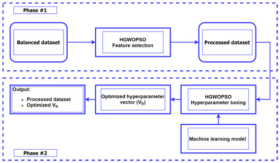
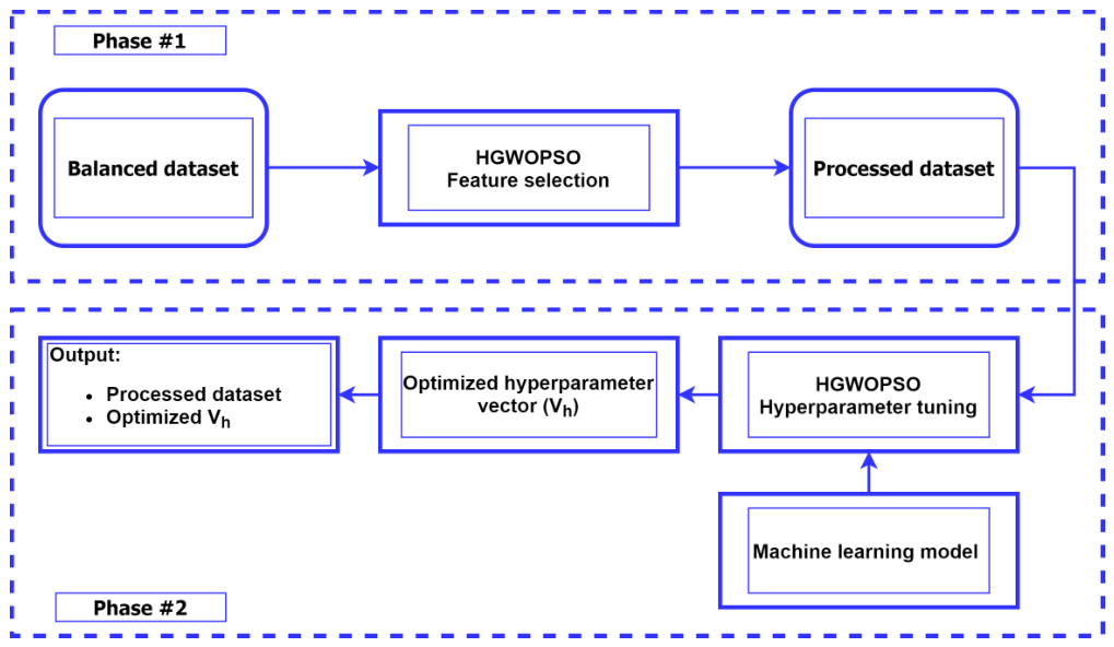
The mechanism of the proposed enhanced detection approach based on the HGWOPSO method is given in Figure 4. The suggested technique has two parts; in the initial phase, the balanced dataset is input into the HGWOPSO algorithm to determine the best features. During the second step, the processed dataset and one of the used machine learning models are inputted into the HGWOPSO algorithm to identify the optimal hyperparameter vector. Table 3 explores the setting of the suggested HGWOPSO algorithm utilized in the trials.

Figure 4. Mechanism of the HGWOPSO-based algorithm for enhanced fault detection.

Table 3. The parameters of the HGWOPSO algorithm.

The Used Algorithm		Variable (s)	Value (s)
HGWOPSO	GWO	a	2 to 0
		# of wolves	20
		# of repetitions	20
	PSO	Inertia $W_{max},W_{min}$	[0.9, 0.6]
		Acceleration constants $C1$, $C2$	[2, 2]
		# of particles	20
		# of generations	20

In this article, due to the large volume of results generated by k-fold cross-validation, it was applied to only one ML model. A k-fold cross-validation procedure with five folds was applied to the TCDJ model, and the corresponding results are presented in Table 4. To prevent data leakage, all preprocessing steps, including SMOTE and feature selection, were applied exclusively to the training set within each fold, while the test data remained entirely unseen during model development. Furthermore, the proposed HGWOPSO optimization process was executed independently within each training fold, ensuring that feature selection and hyperparameter tuning were not influenced by the test data, thereby effectively avoiding data leakage.

Table 4. Five-fold cross-validation results of the TCDJ ML model.

k-Fold	$\mathit{A}$ (%)	$\mathit{P}$ (%)	$\mathit{R}$ (%)	$\mathit{S}$ (%)
1	94.2	93.0	95.2	93.6
2	94.8	93.2	95.3	93.8
3	94.4	93.4	95.5	93.2
4	94.0	93.2	95.3	93.4
5	94.6	93.6	95.1	93.3
$\mu \pm \sigma$	$94.4\pm 0.316$	$93.28\pm 0.228$	$95.28\pm 0.148$	$93.46\pm 0.241$

The k-fold cross-validation results demonstrate that the proposed method achieves stable and consistent performance across different data partitions. As shown in Table 4, the accuracy values range narrowly between 94.0% and 94.8%, with a mean of 94.4% and a low standard deviation of 0.316, indicating minimal variation across folds. Similarly, precision, recall, and F1-score exhibit consistent behavior, with mean values of 93.28%, 95.28%, and 93.46%, respectively, and very small standard deviations. This low variability confirms that the model’s performance is not dependent on a specific train–test split and highlights its robustness and the reliability of the results. Overall, the cross-validation results validate the reliability of the proposed approach for fault detection under varying data distributions.

6. Evaluation Measures

Numerous analytical criteria may be employed to evaluate the efficacy of the binary-based fault detection machine learning technique described [12]. This study used 10 criteria derived from the counts of True Positives (TP), True Negatives (TN), False Positives (FP), and False Negatives (FN). TP represents the count of accurate forecasts for the positive class, TN denotes the count of accurate predictions for the negative class, FP indicates the count of incorrect forecasts within the positive class, and FN signifies the count of erroneous forecasts for the negative class. The indicators are concisely delineated as follows: Table 3 explores the setting of the suggested HGWOPSO algorithm utilized in the trials:

• Accuracy (A) is the ratio of accurate forecasts to the dataset’s total number of forecast samples.

  $$A={\displaystyle \frac{TP+TN}{TP+TN+FP+FN}}$$

  (20)
• Precision (P) is the ratio of true predictions of the positive group to the whole positive predictions. Precision manifests the exactness of the classifier. It can be defined as the rate of accurately identified samples as “faulty” from all samples in the test set to those classified as “faulty.”

  $$P={\displaystyle \frac{TP}{TP+FP}}$$

  (21)
• Recall (R), also referred to as sensitivity; it is the ratio of accurate forecasts of the positive class to the total of accurate forecasts of the positive class and inaccurate forecasts of the negative class. R denotes the classifier’s successful completion.

  $$R={\displaystyle \frac{TP}{TP+FN}}$$

  (22)
• F1 Score (S) is the precision and recall weighted average. S is significantly more practical than accuracy, especially for irregularly distributed data.

  $$S={\displaystyle \frac{2\times P\times R}{P+R}}$$

  (23)
• False Alarm Rate (FAR) is the ratio of incorrect forecasts in the positive class to the total of incorrect forecasts in the positive class and true negatives in the negative class. FAR defines the rate of “non-faulty” samples misclassified as “faulty.”

  $$FAR={\displaystyle \frac{FP}{FP+TN}}$$

  (24)
• Specificity ($S_P$), also called True Negative Rate (TNR), is the ratio of accurate forecasts of the negative class to the total of accurate forecasts of the negative class and inaccurate forecasts of the positive class. Specificity denotes the proportion of correctly identified non-faulty samples among all non-faulty samples.

  $$S_P={\displaystyle \frac{TN}{TN+FP}}$$

  (25)
• False Negative Rate (FNR) is the ratio of inaccurate forecasts in the negative class to the total of inaccurate forecasts in the negative class and accurate forecasts in the positive class. FNR defines the rate of “faulty” samples misclassified as “non-faulty.”

  $$FNR={\displaystyle \frac{FN}{FN+TP}}$$

  (26)
• Matthews Correlation Coefficient (MCC) is a comprehensive metric that utilizes all components of the confusion matrix. It is often utilized for assessing the efficacy of classifiers on unbalanced datasets [54]. The MCC value ranges from −1 to 1, with −1 signifying a completely erroneous classifier and 1 indicating a wholly accurate classifier. MCC can be computed as follows [55].

  $$MCC={\displaystyle \frac{\left(TP\times TN\right)-\left(FP\times FN\right)}{\sqrt{\left(TP+FN\right)\times \left(TP+FP\right)\times \left(TN+FP\right)\times \left(TN+FN\right)}}}$$

  (27)
• The area under the ROC curve (AUC) is a quantitative metric that represents the ROC curve [56]. The AUC value ranges from 0 to 1, indicating that a greater AUC signifies superior classifier performance. The AUC may be computed as below [57]:

  $$AUC={\displaystyle \frac{1}{2}}\times \left(TPR+TNR\right)$$

  (28)
• Average Fitting Value (AFV) AFV is employed to average the most significant parameters equitably. In AFV, all measures possess equal significance in the numerator; hence, the weight assigned to each metric is 1. The main objective of employing such an average metric is to rank classifiers according to their total efficacy. The general equation of AFV based on AUC, TNR, FAR, and FNR is given as follows:

  $$AFV={\displaystyle \frac{AUC+TNR+(1-FAR)+(1-FNR)}{4}}$$

  (29)

7. Results and Discussion

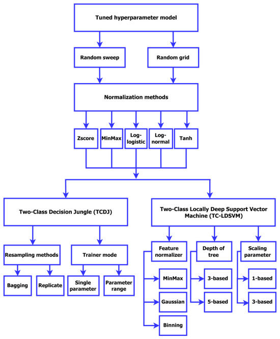
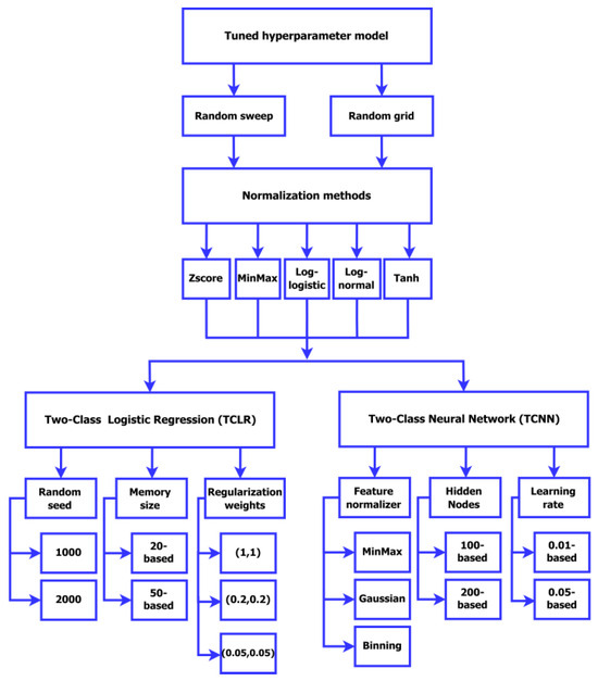
The VSB-ENET raw data are organized into “CSV” files using Python 3.12.4 [58] and a co-laboratory online tool created by Google [59]. The presented HGWOPSO algorithm is also developed in Python. All remaining phases depicted in Figure 3, including data preprocessing, data pre-training, data training, and data testing, are implemented by the cloud-based AMLS platform [60]. This platform is an effective tool for developing and evaluating machine learning models. Figure 5 and Figure 6 illustrate all machine learning models considering all parameters are investigated to determine the most parameters affect the model’s performance.

Figure 5. Flowchart of the first and second scenarios.

Figure 6. Flowchart of the third and fourth scenarios.

The successful performance of any model primarily relies on its attained assessment metrics score. Higher values in A, P, R, S, $S_P$, and MCC, and lower values in FAR and FNR indicate an effective classifier. The optimal classifier achieves A and R values of one, while the FAR value is zero. Our proposed method is applied to the four machine learning models and four scenarios are constructed as given in Figure 5 and Figure 6. Figure 5 and Figure 6 show all the combinations of the machine learning models’ parameters.

7.1. Impact of Normalization Type

Table 5, Table 6, Table 7 and Table 8 provide all the results of the proposed scenarios. Examining Table 5, the TCDJ training method based on different normalization and hyperparameter tuning methods is studied. Two resampling methods are used, bagging and replicate. Also, two training modes are utilized, single and parameter range. The other parameters such as $N_d$, $D_m$, $D_w$, and $N_s$ are adjusted as shown in Table 5. The suggested improved detection method is implemented on the four machine learning models referenced in Section 5.5, and the evaluation metrics outlined in Section 6 are computed appropriately. The highlighted and underlined values denote the models’ optimal outcomes within the same experiment and across all experiments, respectively. Moreover, it is evident that TCDJ, utilizing log-logistic normalization and a random sweep tuning strategy, attained superior performance across all evaluation metrics and execution time. The AFV was 95.15%, while the running time was about 185 s. The TCDJ model based on Z-score and Min–Max normalization methods also achieved high performance. Investigating Table 6, TC-LDSVM model based on Z-score normalization accomplished the best performance with about 97% AFV. Further, the TC-LDSVM model based on Min–Max normalization came in the first rank in terms of time computations with about 113 s and the second rank of better performance with approximately 96% AFV. Inspecting Table 7, the TCLR model based on Z-score achieved the highest AFV (80.47%). Moreover, the TCLR model based on Min–Max achieved the second-highest AFV (80.38%). Examining Table 8, the TCNN model based on Z-score normalization realized the highest performance with about 96.63% AFV. In addition, the TCNN model based on Min–Max normalization achieved high performance (95.84%) within the least time computation at all (0.6 s).

Table 5. Results of Scenario #1.

Machine Learning Model	TP	TN	FP	FN	A (%)	P (%)	R (%)	S (%)	AUC (%)	FAR (%)	TNR (%)	FNR (%)	Running Time (s)	AFV (%)
Random Sweep (Bagging, Single parameter, 8, 32, 128, 2048)
TCDJ(Z-score)	2249	2288	168	113	94.2	93.0	95.2	93.6	98.6	6.8	93.2	4.8	214.8	95.03
TCDJ(Min–Max)	2249	2288	168	113	94.2	93.0	95.2	93.6	98.6	6.8	93.2	4.8	189.6	95.03
TCDJ(Log-logistic)	2252	2266	190	110	93.8	92.2	95.3	93.0	98.5	7.7	92.3	4.7	192.0	94.59
TCDJ(Log-normal)	2177	2169	287	185	90.2	88.4	92.2	89.3	96.4	11.7	88.3	7.8	187.2	91.30
TCDJ(Tanh)	2193	2242	214	169	92.1	91.1	92.8	91.6	97.8	8.7	91.3	7.2	191.4	93.30
Random Sweep (Replicate, Single parameter, 8, 32, 128, 2048)
TCDJ(Z-score)	2246	2286	170	116	94.1	93.0	95.1	93.5	98.6	6.9	93.1	4.9	222.6	94.96
TCDJ(Min–Max)	2246	2286	170	116	94.1	93.0	95.1	93.5	98.6	6.9	93.1	4.9	186.0	94.96
TCDJ(Log-logistic)	2251	2290	166	111	94.3	93.1	95.3	93.7	98.8	6.8	93.2	4.7	188.4	95.15
TCDJ(Log-normal)	2180	2189	267	182	90.7	89.1	92.3	89.9	96.9	10.9	89.1	7.7	185.4	91.86
TCDJ(Tanh)	2192	2218	238	170	91.5	90.2	92.8	90.9	97.6	9.7	90.3	7.2	189.0	92.76
Random Grid (Bagging, Single Parameter, 8, 32, 128, 2048)
TCDJ(Z-score)	2249	2288	168	113	94.2	93.0	95.2	93.6	98.6	6.8	93.2	4.8	431.4	95.03
TCDJ(Min–Max)	2249	2288	168	113	94.2	93.0	95.2	93.6	98.6	6.8	93.2	4.8	423.0	95.03
TCDJ(Log-logistic)	2252	2266	190	110	93.8	92.2	95.3	93.0	98.5	7.7	92.3	4.7	450.0	94.59
TCDJ(Log-normal)	2177	2169	287	185	90.2	88.4	92.2	89.3	96.4	11.7	88.3	7.8	378.6	91.30
TCDJ(Tanh)	2193	2242	214	169	92.1	91.1	92.8	91.6	97.8	8.7	91.3	7.2	378.0	93.30
Random Sweep (Bagging, Parameter Range, (1, 8, 32), (1, 16, 64), (1, 128, 1024), (1024, 4096, 16,384))
TCDJ(Z-score)	2249	2288	168	113	94.2	93.0	95.2	93.6	98.6	6.8	93.2	4.8	298.8	95.03
TCDJ(Min–Max)	2249	2288	168	113	94.2	93.0	95.2	93.6	98.6	6.8	93.2	4.8	292.2	95.03
TCDJ(Log-logistic)	2252	2266	190	110	93.8	92.2	95.3	93.0	98.5	7.7	92.3	4.7	295.2	94.59
TCDJ(Log-normal)	2177	2169	287	185	90.2	88.4	92.2	89.3	96.4	11.7	88.3	7.8	243.6	91.30
TCDJ(Tanh)	2193	2242	214	169	92.1	91.1	92.8	91.6	97.8	8.7	91.3	7.2	273.6	93.30
Random Sweep (Replicate, Parameter Range, (1, 8, 32), (1, 16, 64), (1, 128, 1024), (1024, 4096, 16,384))
TCDJ(Z-score)	2249	2288	168	113	94.2	93.0	95.2	93.6	98.6	6.8	93.2	4.8	298.2	95.03
TCDJ(Min–Max)	2249	2288	168	113	94.2	93.0	95.2	93.6	98.6	6.8	93.2	4.8	307.2	95.03
TCDJ(Log-logistic)	2252	2266	190	110	93.8	92.2	95.3	93.0	98.5	7.7	92.3	4.7	297.6	94.59
TCDJ(Log-normal)	2177	2169	287	185	90.2	88.4	92.2	89.3	96.4	11.7	88.3	7.8	248.4	91.30
TCDJ(Tanh)	2193	2242	214	169	92.1	91.1	92.8	91.6	97.8	8.7	91.3	7.2	288.0	93.30

Table 6. Results of Scenario #2.

Machine Learning Model	TP	TN	FP	FN	A (%)	P (%)	R (%)	S (%)	AUC (%)	FAR (%)	TNR (%)	FNR (%)	Running Time (s)	AFV (%)
Random Sweep (Single, 3, 0.1, 0.01, 0.01, 1, 15,000, Min–Max normalizer, 1000)
TC-LDSVM (Z-score)	2113	1947	509	249	84.3	80.6	89.5	82.4	92.4	20.7	79.3	10.5	157.8	85.10
TC-LDSVM (Min–Max)	2030	2059	397	332	84.9	83.6	85.9	84.3	93.0	16.2	83.8	14.1	129.0	86.65
TC-LDSVM (Log-logistic)	1603	1890	566	759	72.5	73.9	67.9	73.2	82.5	23.0	77.0	32.1	138.0	76.07
TC-LDSVM (Log-normal)	-	-	-	-	-	-	-	-	-	-	-	-	-	-
TC-LDSVM (Tanh)	1621	1904	552	741	73.2	74.6	68.6	73.9	82.8	22.5	77.5	31.4	135.6	76.62
Random Sweep (Single, 5, 0.1, 0.01, 0.01, 3, 15,000, Min–Max normalizer, 1000)
TC-LDSVM (Z-score)	2092	2039	417	270	85.7	83.4	88.6	84.5	93.7	17.0	83.0	11.4	139.2	87.08
TC-LDSVM (Min–Max)	2095	2003	453	267	85.1	82.2	88.7	83.6	93.2	18.4	81.6	11.3	139.2	86.25
TC-LDSVM (Log-logistic)	1908	1658	798	454	74.0	70.5	80.8	72.2	83.4	32.5	67.5	19.2	178.8	74.80
TC-LDSVM (Log-normal)	-	-	-	-	-	-	-	-	-	-	-	-	-	-
TC-LDSVM (Tanh)	1971	1526	930	391	72.6	67.9	83.4	70.2	80.8	37.9	62.1	16.6	184.8	72.13
Random Sweep (Single, 3, 0.1, 0.01, 0.01, 1, 15,000, Gaussian normalizer, 1000)
TC-LDSVM (Z-score)	2227	2393	63	135	95.9	97.2	94.3	96.6	98.7	2.6	97.4	5.7	119.4	96.96
TC-LDSVM (Min–Max)	2218	2340	116	144	94.6	95.0	93.9	94.8	98.5	4.7	95.3	6.1	112.8	95.74
TC-LDSVM (Log-logistic)	1790	2146	310	572	81.7	85.2	75.8	83.4	90.7	12.6	87.4	24.2	150.6	85.31
TC-LDSVM (Log-normal)	-	-	-	-	-	-	-	-	-	-	-	-	-	-
TC-LDSVM (Tanh)	1773	2147	309	589	81.4	85.2	75.1	83.2	89.2	12.6	87.4	24.9	153.0	84.78
Random Sweep (Single, 3, 0.1, 0.01, 0.01, 1, 15,000, Binning normalizer, 1000)
TC-LDSVM (Z-score)	2147	2220	236	215	90.6	90.1	90.9	90.4	96.0	9.6	90.4	9.1	128.4	91.92
TC-LDSVM (Min–Max)	2167	2142	314	195	89.4	87.3	91.7	88.4	95.9	12.8	87.2	8.3	125.4	90.52
TC-LDSVM (Log-logistic)	2116	2184	272	246	89.2	88.6	89.6	88.9	96.0	11.1	88.9	10.4	118.2	90.86
TC-LDSVM (Log-normal)	-	-	-	-	-	-	-	-	-	-	-	-	-	-
TC-LDSVM (Tanh)	1619	2092	364	743	77.0	81.6	68.5	79.3	84.6	14.8	85.2	31.5	121.2	80.88

Table 7. Results of Scenario #3.

Machine Learning Model	TP	TN	FP	FN	A (%)	P (%)	R (%)	S (%)	AUC (%)	FAR (%)	TNR (%)	FNR (%)	Running Time (s)	AFV (%)
Random Sweep (Single, 1xE-7, 1, 1, 20, 1000)
TCLR (Z-score)	1732	1884	572	630	75.1	75.2	73.3	75.1	81.5	23.3	76.7	26.7	45.0	77.06
TCLR (Min–Max)	1735	1880	576	627	75.0	75.1	73.5	75.1	81.5	23.5	76.5	26.5	21.6	77.01
TCLR (Log-logistic)	1234	1724	732	1128	61.4	62.8	52.2	62.1	63.6	29.8	70.2	47.8	15.0	64.06
TCLR (Log-normal)	-	-	-	-	-	-	-	-	-	-	-	-	-	-
TCLR (Tanh)	1152	1753	703	1210	60.3	62.1	48.8	61.2	63.3	28.6	71.4	51.2	15.0	63.71
Random Grid (Single, 1xE-7, 1, 1, 20, 1000)
TCLR (Z-score)	1732	1884	572	630	75.1	75.2	73.3	75.1	81.4	23.3	76.7	26.7	14.4	77.04
TCLR (Min–Max)	1735	1880	576	627	75.0	75.1	73.5	75.1	81.5	23.5	76.5	26.5	12.6	77.01
TCLR (Log-logistic)	1234	1724	732	1128	61.4	62.8	52.2	62.1	63.6	29.8	70.2	47.8	10.8	64.06
TCLR (Log-normal)	-	-	-	-	-	-	-	-	-	-	-	-	-	-
TCLR (Tanh)	1152	1753	703	1210	60.3	62.1	48.8	61.2	63.3	28.6	71.4	51.2	14.4	63.71
Random Sweep (Single, 1xE-7, 1, 1, 50, 1000)
TCLR (Z-score)	1731	1886	570	631	75.1	75.2	73.3	75.2	81.5	23.2	76.8	26.7	45.0	77.09
TCLR (Min–Max)	1733	1883	573	629	75.1	75.2	73.4	75.1	81.4	23.3	76.7	26.6	15.0	77.03
TCLR (Log-logistic)	1229	1730	726	1133	61.4	62.9	52.0	62.1	63.5	29.6	70.4	48.0	43.8	64.10
TCLR (Log-normal)	-	-	-	-	-	-	-	-	-	-	-	-	-	-
TCLR (Tanh)	1151	1753	703	1211	60.3	62.1	48.7	61.2	63.3	28.6	71.4	51.3	44.4	63.70
Random Sweep (Single, 1xE-7, 0.2, 0.2, 20, 1000)
TCLR (Z-score)	1745	1957	499	617	76.8	77.8	73.9	77.3	84.0	20.3	79.7	26.1	21.6	79.31
TCLR (Min–Max)	1747	1953	503	615	76.8	77.6	74.0	77.2	84.0	20.5	79.5	26.0	15.0	79.25
TCLR (Log-logistic)	1205	1735	721	1157	61.0	62.6	51.0	61.8	63.4	29.4	70.6	49.0	49.2	63.93
TCLR (Log-normal)	-	-	-	-	-	-	-	-	-	-	-	-	-	-
TCLR (Tanh)	1154	1748	708	1208	60.2	62.0	48.9	61.1	63.3	28.8	71.2	51.1	42.6	63.63
Random Sweep (Single, 1xE-7, 0.05, 0.05, 20, 2000)
TCLR (Z-score)	1748	2004	452	614	77.9	79.5	74.0	78.7	84.7	18.4	81.6	26.0	24.0	80.47
TCLR (Min–Max)	1745	2001	455	617	77.8	79.3	73.9	78.5	84.7	18.5	81.5	26.1	39.6	80.38
TCLR (Log-logistic)	1204	1737	719	1158	61.0	62.6	51.0	61.8	63.5	29.3	70.7	49.0	15.6	63.98
TCLR (Log-normal)	-	-	-	-	-	-	-	-	-	-	-	-	-	-
TCLR (Tanh)	1153	1714	742	1209	59.5	60.8	48.8	60.2	63.3	30.2	69.8	51.2	18.0	62.92

Table 8. Results of Scenario #4.

Machine Learning Model	TP	TN	FP	FN	A (%)	P (%)	R (%)	S (%)	AUC (%)	FAR (%)	TNR (%)	FNR (%)	Running Time (s)	AFV (%)
Random Sweep (Single, Fully-connected, 100, 0.1, 100, 0.1, 0, Min–Max normalizer, 1000)
TCNN (Z-score)	2129	2202	254	233	89.9	89.3	90.1	89.6	97.2	10.3	89.7	9.9	104.4	91.66
TCNN (Min–Max)	2129	2202	254	233	89.9	89.3	90.1	89.6	97.2	10.3	89.7	9.9	67.8	91.66
TCNN (Log-logistic)	1649	1935	521	713	74.4	76.0	69.8	75.2	83.5	21.2	78.8	30.2	102.6	77.72
TCNN (Log-normal)	-	-	-	-	-	-	-	-	-	-	-	-	-	-
TCNN (Tanh)	1618	1918	538	744	73.4	75.0	68.5	74.2	83.2	21.9	78.1	31.5	72.0	76.97
Random Grid (Single, Fully-connected, 100, 0.1, 100, 0.1, 0, Min–Max normalizer, 1000)
TCNN (Z-score)	2129	2202	254	233	89.9	89.3	90.1	89.6	97.2	10.3	89.7	9.9	87.0	91.66
TCNN (Min–Max)	2129	2202	254	233	89.9	89.3	90.1	89.6	97.2	10.3	89.7	9.9	62.4	91.66
TCNN (Log-logistic)	1649	1935	521	713	74.4	76.0	69.8	75.2	83.5	21.2	78.8	30.2	100.8	77.72
TCNN (Log-normal)	-	-	-	-	-	-	-	-	-	-	-	-	-	-
TCNN (Tanh)	1618	1918	538	744	73.4	75.0	68.5	74.2	83.2	21.9	78.1	31.5	89.4	76.97
Random Sweep (Single, Fully-connected, 100, 0.1, 100, 0.1, 0, Gaussian normalizer, 1000)
TCNN (Z-score)	2255	2357	99	107	95.7	95.8	95.5	95.8	99.1	4.0	96.0	4.5	77.4	96.63
TCNN (Min–Max)	2226	2349	107	136	95.0	95.4	94.2	95.2	98.8	4.4	95.6	5.8	72.0	96.08
TCNN (Log-logistic)	1610	2438	18	752	84.0	98.9	68.2	90.9	92.3	0.7	99.3	31.8	73.2	89.75
TCNN (Log-normal)	-	-	-	-	-	-	-	-	-	-	-	-	-	-
TCNN (Tanh)	1533	2429	27	829	82.2	98.3	64.9	89.5	90.5	1.1	98.9	35.1	66.6	88.30
Random Sweep (Single, Fully-connected, 100, 0.1, 100, 0.1, 0, Binning normalizer, 1000)
TCNN (Z-score)	2203	2349	107	159	94.5	95.4	93.3	94.9	98.8	4.4	95.6	6.7	148.8	95.84
TCNN (Min–Max)	2202	2349	107	160	94.5	95.4	93.2	94.9	98.8	4.4	95.6	6.8	112.2	95.83
TCNN (Log-logistic)	2197	2280	176	165	92.9	92.6	93.0	92.8	98.2	7.2	92.8	7.0	90.0	94.22
TCNN (Log-normal)	-	-	-	-	-	-	-	-	-	-	-	-	-	-
TCNN (Tanh)	1701	2083	373	661	78.5	82.0	72.0	80.2	87.0	15.2	84.8	28.0	98.4	82.16
Random Sweep (Single, Fully-connected, 200, 0.05, 100, 0.1, 0, Min–Max normalizer, 1000)
TCNN (Z-score)	2203	2349	107	159	94.5	95.4	93.3	94.9	98.8	4.4	95.6	6.7	1.2	95.84
TCNN (Min–Max)	2202	2349	107	160	94.5	95.4	93.2	94.9	98.8	4.4	95.6	6.8	0.6	95.83
TCNN (Log-logistic)	2197	2280	176	165	92.9	92.6	93.0	92.8	98.2	7.2	92.8	7.0	19.2	94.22
TCNN (Log-normal)	-	-	-	-	-	-	-	-	-	-	-	-	-	-
TCNN (Tanh)	1701	2083	373	661	78.5	82.0	72.0	80.2	87.0	15.2	84.8	28.0	1.2	82.16

The top-ranking of the models from the best to the worst was TC-LDSVM Z-score-based, TCNN Z-score-based, TCDJ Log-logistic-based, and TCLR Z-score-based, respectively. However, TCLR was the worst in terms of performance; it was the best model among the four machine learning models in terms of computation complexity.

7.2. Impact of Feature Selection and Hyperparameter Tuning Optimization Method

This section presents a comparative analysis of four ML models, considering both baseline configurations without hyperparameter optimization and optimized configurations employing the proposed HGWOPSO optimization method. Table 9 compares the baseline models with their HGWOPSO-enabled counterparts. The comparison is conducted in terms of AUC, AFV, $T_{training}$, and $T_{testing}$. The HGWOPSO-based TCDJ, TC-LDSVM, TCLR, and TCNN models outperform their baseline versions in terms of AUC and AFV. However, these performance improvements are achieved at the cost of increased computational complexity during both training and testing phases. Specifically, for the TCDJ model, the HGWOPSO-enabled configuration improves AUC and AFV by 10.0% and 9.4%, respectively, compared with the baseline model. Also, different optimization methods, such as GWO [33], PSO [61], GA [62], WOA [63], MVO [64], and FA [65], were compared to the proposed HGWOPSO optimization method. Table 10 provides the parameters of each optimization method. These optimization techniques were employed on the VSB-ENET dataset to identify the most significant features and optimize the hyperparameters of every training model. Table 11 shows the values of AUC and MCC metrics, and the number of selected features ($N_f$) for each optimization method in comparison to the proposed HGWOPSO method. It can be observed that the proposed HGWOPSO method not only outperforms the other feature selection techniques in terms of predictive performance, but also achieves this while selecting the smallest feature subset. It can be observed that the proposed HGWOPSO method outperformed all the other methods for all training models. Additionally, HGWOPSO utilizing the TCNN training model achieved optimal performance, evidenced by an AUC of 99.10% and an MCC of 91.45%. Also, HGWOPSO with the TCDJ training model achieved good performance with 98.80% and 88.53% for AUC and MCC, respectively. GWO method also occupied the second rank after HGWOPSO with 96.62% and 87.65% for AUC and MCC, respectively.

Table 9. Comparative analysis of ML models considering HGWOPSO-enabled and HGWOPSO-disabled configurations.

Algorithm	Model	AUC (%)	AFV (%)	T_training (s)	T_testing (s)
HGWOPSO-disabled	TCDJ Random Sweep, (Replicate, Single parameter, 8, 32, 128, 2048), (Log-logistic)	89.8	86.2	162.3	92.6
	TC-LDSVM Random Sweep (Single, 3, 0.1, 0.01, 0.01, 1, 15,000, Gaussian normalizer, 1000), (Z-score)	89.6	85.7	104.2	48.6
	TCLR Random Sweep (Single, 1xE-7, 0.05, 0.05, 20, 2000), (Z-score)	78.5	73.8	17.6	10.8
	TCNN Random Sweep (Single, Fully-connected, 100, 0.1, 100, 0.1, 0, Gaussian normalizer, 1000), (Z-score)	90.2	88.3	59.5	29.4
HGWOPSO-enabled	TCDJ	98.8	95.15	188.4	103.6
	TC-LDSVM	98.7	96.96	119.4	67.2
	TCLR	84.7	80.47	24	13.4
	TCNN	99.1	96.63	77.4	37.6

Table 10. Configuration of algorithms for feature selection and hyperparameter optimization.

The Used Algorithm	Parameter (s)	Value (s)
GWO	a	[0, 2]
	# of wolves	30
	# of iterations	30
PSO	Inertia Wmin, Wmax	[0.6, 0.9]
	Variables of accelerating C1, C2	2
	# of particles	30
	# of generations	30
GA	Rate of mutation	0.1
	Crossover	0.9
	Population size	30
	# of generations	30
WOA	a	[0, 2]
	r	[0, 1]
	Whales number	30
	Iterations number	30
MVO	Probability of wormhole existence	[0.1, 1]
FA	Fireflies number	30

Table 11. Compared algorithms when applied on feature selection and hyperparameter tuning.

Machine Learning Model	Parameters of Machine Learning Model	Metric	Algorithms
			GWO	PSO	GA	WOA	MVO	FA	HGWOPSO
TCDJ	Random Sweep (Replicate, Single parameter, $N_d=8$, $D_m=32$, $D_w=128$, $N_s=2048$)	AUC	96.52	94.45	95.92	95.40	95.85	94.60	98.80
		MCC	86.36	84.25	86.20	85.30	85.64	84.75	88.53
		$N_f$	15	16	15	15	15	16	14
TC-LDSVM	Random Sweep (Single, $D_t=3$, ${\lambda }_w=0.1$, ${\lambda }_{\theta }=0.01$, ${\widehat{\lambda }}_{\theta }=0.01$, ${\sigma }_s=1$, N = 15,000, Gaussian normalizer, $R_s=1000$)	AUC	96.24	93.76	95.80	95.34	95.45	94.10	98.70
		MCC	87.70	84.68	86.50	86.25	86.45	85.21	91.81
		$N_f$	15	17	15	15	15	16	13
TCLR	Random Sweep (Single, $ϵ=1\times {10}^{-7}$, ${\lambda }_{w1}=0.05$, ${\lambda }_{w2}=0.05$, $M_s=20$, $R_s=2000$)	AUC	81.26	77.36	81.15	79.15	79.45	78.62	84.70
		MCC	48.22	43.96	47.35	45.36	46.20	44.68	55.88
		$N_f$	16	18	17	17	17	16	15
TCNN	Random Sweep (Single, Fully-connected, $N_h=100$, $\alpha =0.1$, $N_l=100$, 0.1, 0, Gaussian normalizer, $R_s=1000$)	AUC	96.62	93.12	96.32	94.66	95.28	93.28	99.10
		MCC	87.65	84.35	87.33	85.89	86.24	84.55	91.45
		$N_f$	12	15	14	15	14	15	11

7.3. ROC Evaluation

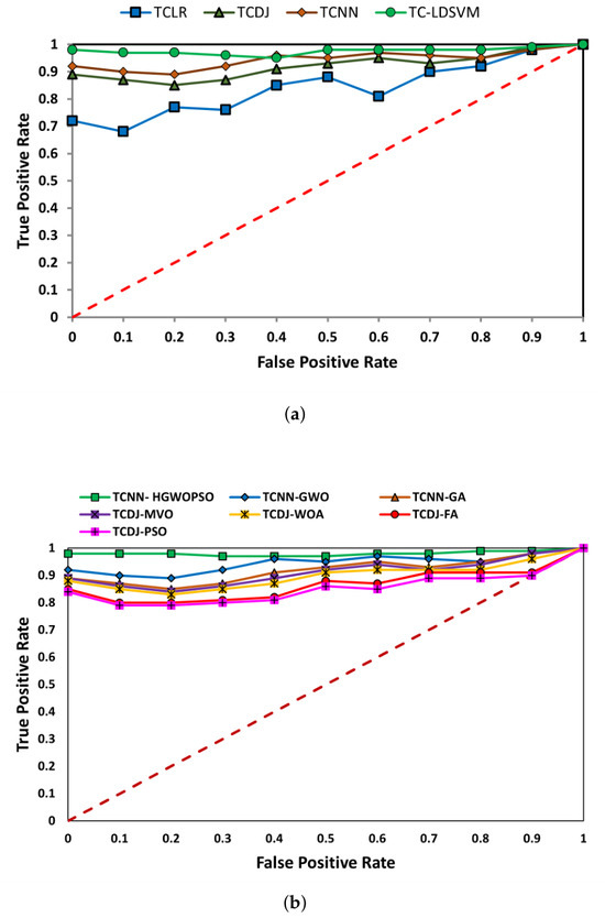
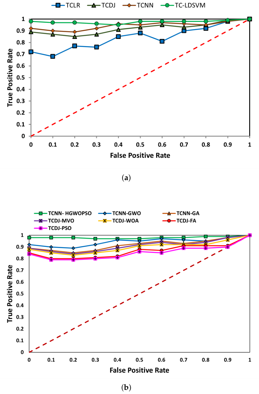
Receiver operating characteristic (ROC) curves are a proficient technique for illustrating and calculating the Area Under the ROC Curve (AUC). ROC is a graphical representation that demonstrates the performance efficacy of a binary classifier. The x-axis of the ROC curve represents the FPR, while the y-axis represents the TPR. The linear trajectory or the dashed line connecting the coordinates (0,0) and (1,1) signifies the 50% performance threshold, as the classifier’s curve converges towards the top-left quadrant of the ROC curve, indicating optimal performance. Figure 7a illustrates the ROC curves representing the average performance of the four training models employed, whereas Figure 7b depicts the ROC curves reflecting the average performance of the optimization approaches. The graphs indicate that HGWOPSO surpassed the other optimization techniques.

Figure 7. ROC curves: (a) comparison between the training machine learning models, and (b) comparison between the optimization methods.

7.4. Comparison with Previous Works

To assess the suitability and applicability of the suggested approach for fault detection in power systems. Our suggested methodology was evaluated against several prior research that employed the identical VSB-ENET dataset [8,18,66]. Table 12 presents a comparison of the fundamental assessment measures. It can be noticed that the proposed HGWOPSO method accomplished significant improvements in all metrics compared to methods in [18,66], whereas it had comparable results compared to methods in [8]. For instance, the (P, R, S) using the TL-LDSVM HGWOPSO-based model were improved by (29.6%, 29.2%, 34.2%) and (20%, 16.4%, 16.4%) compared to the STL-SVM RBF kernel and PD methods, respectively. The findings of this study indicate that the suggested technique effectively detects faults in power systems, particularly in modern and complex grids.

Table 12. Comparing the performance with previous studies.

Reference	Suggested Method	A	P	R	S	AUC	MCC
[66]	STL + SVM (Linear Kernel)	-	0.720	0.700	0.700	-	-
	STL + SVM (Polynomial Kernel with 6 Degrees)	-	0.670	0.550	0.450	-	-
	STL + SVM (RBF Kernel)	-	0.750	0.730	0.720	-	-
	STL + SVM (Sigmoid Kernel)	-	0.530	0.520	0.500	-	-
[18]	Non-PD Signals	-	0.810	0.810	0.810	-	-
	PD Signals	-	0.810	0.810	0.830	-	-
[8]	1-Phase Optimized Threshold	0.953	0.669	0.844	-	-	-
	3-Phase Global Threshold	0.967	0.726	0.957	-	-	-
This Study	Random Sweep (Replicate, Single parameter, $N_d=8$, $D_m=32$, $D_w=128$, $N_s=2048$) TCDJ-based	0.943	0.931	0.953	0.937	0.988	0.885
	Random Sweep (Single, $D_t=3$, ${\lambda }_w=0.1$, ${\lambda }_{\theta }=0.01$, ${\widehat{\lambda }}_{\theta }=0.01$, ${\sigma }_s=1$, N = 15,000, Gaussian normalizer, $R_s=1000$) TC-LDSVM-based	0.959	0.972	0.943	0.966	0.987	0.918
	Random Sweep (Single, Fully-connected, $N_h=100$, $\alpha =0.1$, $N_l=100$, 0.1, 0, Gaussian normalizer, $R_s=1000$) TCNN-based	0.957	0.958	0.955	0.958	0.991	0.915

Note: STL = Seasonal and trend decomposition using Loess; RBF = Radial Basis Function; PD = partial discharge.

8. Conclusions

The complexity of modern power systems and the tendency of utilities to modernize their grids to smart configurations render fault identification increasingly difficult. This article presents an innovative fault detection method aimed at identifying faults in modern power grids and addressing the limitations of traditional fault detection techniques. The suggested two-class classification method employs four machine learning models to improve fault detection performance. The enhancements were carried out over two phases, feature selection and hyperparameter tuning via the novel HGWOPSO method. This article utilized the actual fault identification dataset developed by the ENET Laboratory at VSB University. The original imbalanced data comprised 94% normal and 6% faulty. The data were equilibrated using the SMOTE approach, resulting in a balanced distribution of 51% normal and 49% faulty instances. The findings from the balanced dataset were compared to those from the unbalanced dataset using several performance assessment measures. Clearly, there were notable improvements in all assessment criteria; for example, AUC, FAR, and FNR were enhanced by 44.5%, 95.2%, and 96.3%, respectively. Feature selection and hyperparameter tuning were optimized via many optimization methods such as GWO, PSO, GA, WOA, MVO, and FA algorithms and compared to the proposed HGWOPSO method. The suggested HGWOPSO approach, utilizing four machine learning models, outperformed the performance of other methods. For example, HGWOPSO enhanced the (AUC, MCC) by (2.6%, 4.3%) and (6.4%, 8.0%) compared to GWO and PSO. The proposed approach was compared to former studies, and its supremacy was confirmed. On the other hand, the proposed HGWOPSO was computationally complex during the training stage due to the hybrid optimization of feature selection and hyperparameter tuning, which may restrict its applicability in scarce-resource environments. In addition, the study was validated on single real dataset, which may affect the generalizability of the results; therefore, applying the proposed method to multiple datasets may further confirm its applicability and generality. Finally, the SMOTE technique was employed to balance the utilized data; however, real-world data fault detection scenarios involve highly imbalanced class distribution which require more robustness tests.

References

- Abid, A.; Khan, M.T.; Iqbal, J. A review on fault detection and diagnosis techniques: Basics and beyond. Artif. Intell. Rev. 2020, 54, 3639–3664. [Google Scholar] [CrossRef] [Scilit]
- Chen, K.; Huang, C.; He, J. Fault detection, classification and location for transmission lines and distribution systems: A review on the methods. High Volt. 2016, 1, 25–33. [Google Scholar] [CrossRef] [Scilit]
- Yu, S.L.; Gu, J.C. Removal of decaying DC in current and voltage signals using a modified Fourier filter algorithm. IEEE Trans. Power Deliv. 2001, 16, 372–379. [Google Scholar] [CrossRef] [Scilit]
- Mallat, S. A Wavelet Tour of Signal Processing; Elsevier: Amsterdam, The Netherlands, 1999. [Google Scholar]
- Thukaram, D.; Khincha, H.; Vijaynarasimha, H. Artificial neural network and support vector machine approach for locating faults in radial distribution systems. IEEE Trans. Power Deliv. 2005, 20, 710–721. [Google Scholar] [CrossRef] [Scilit]
- Jiang, J.A.; Yang, J.Z.; Lin, Y.H.; Liu, C.W.; Ma, J.C. An adaptive PMU based fault detection/location technique for transmission lines. I. Theory and algorithms. IEEE Trans. Power Deliv. 2000, 15, 486–493. [Google Scholar] [CrossRef] [Scilit]
- Zin, A.A.M.; Saini, M.; Mustafa, M.W.; Sultan, A.R. New algorithm for detection and fault classification on parallel transmission line using DWT and BPNN based on Clarke’s transformation. Neurocomputing 2015, 168, 983–993. [Google Scholar] [CrossRef] [Scilit]
- Michau, G.; Hsu, C.C.; Fink, O. Interpretable detection of partial discharge in power lines with deep learning. Sensors 2021, 21, 2154. [Google Scholar] [CrossRef] [Scilit]
- Jamil, M.; Sharma, S.K.; Singh, R. Fault detection and classification in electrical power transmission system using artificial neural network. SpringerPlus 2015, 4, 334. [Google Scholar] [CrossRef] [Scilit]
- Xu, L.; Chow, M.Y.; Taylor, L.S. Power distribution fault cause identification with imbalanced data using the data mining-based fuzzy classification e-algorithm. IEEE Trans. Power Syst. 2007, 22, 164–171. [Google Scholar] [CrossRef] [Scilit]
- Wang, H.; Keerthipala, W. Fuzzy-neuro approach to fault classification for transmission line protection. IEEE Trans. Power Deliv. 1998, 13, 1093–1104. [Google Scholar] [CrossRef] [Scilit]
- Tag Eldin, E.S. Fault location for a series compensated transmission linebased on wavelet transform and an adaptive neuro-fuzzy inference system. In Proceedings of the Electric Power Quality and Supply Reliability Conference (PQ), Berg, Estonia, 16–18 June 2010; pp. 229–236. [Google Scholar]
- Meyur, R.; Pal, D.; Sundaravaradan, N.a.; Rajaraman, P.; Srinivas, K.; Reddy, M.J.B.; Mohanta, D. A wavelet-adaptive network based fuzzy inference system for location of faults in parallel transmission lines. In Proceedings of the 2016 IEEE International Conference on Power Electronics, Drives and Energy Systems (PEDES); IEEE: Piscataway, NJ, USA, 2016; pp. 1–6. [Google Scholar]
- Othman, M.; Mahfouf, M.; Linkens, D. Transmission lines fault detection, classification and location using an intelligent power system stabiliser. In Proceedings of the 2004 IEEE International Conference on Electric Utility Deregulation, Restructuring and Power Technologies; IEEE: Piscataway, NJ, USA, 2004; Volume 1, pp. 360–365. [Google Scholar]
- Eboule, P.S.P.; Pretorius, J.H.C.; Mbuli, N.; Leke, C. Fault detection and Location in power transmission line using concurrent neuro fuzzy technique. In Proceedings of the 2018 IEEE Electrical Power and Energy Conference (EPEC); IEEE: Piscataway, NJ, USA, 2018; pp. 1–6. [Google Scholar]
- Hu, Z.; Liu, S.; Luo, W.; Wu, L. Intrusion-detector-dependent distributed economic model predictive control for load frequency regulation with PEVs under cyber attacks. IEEE Trans. Circuits Syst. I Regul. Pap. 2021, 68, 3857–3868. [Google Scholar] [CrossRef] [Scilit]
- Wadi, M. Fault Detection in Power Grids Based on Improved Supervised Machine Learning Binary Classification. J. Electr. Eng. 2021, 72, 217–228. [Google Scholar] [CrossRef] [Scilit]
- Qu, N.; Li, Z.; Zuo, J.; Chen, J. Fault detection on insulated overhead conductors based on DWT-LSTM and partial discharge. IEEE Access 2020, 8, 87060–87070. [Google Scholar] [CrossRef] [Scilit]
- Elmasry, W.; Wadi, M. Detection of faults in electrical power grids using an enhanced anomaly-based method. Arab. J. Sci. Eng. 2022, 47, 14899–14914. [Google Scholar] [CrossRef] [Scilit]
- Wadi, M.; Elmasry, W.; Colak, I.; Jouda, M.; Kucuk, I. Utilizing Metaheuristics to Estimate Wind Energy Integration in Smart Grids with A Comparative Analysis of Ten Distributions. Electr. Power Compon. Syst. 2024, 1–36. [Google Scholar] [CrossRef] [Scilit]
- Elmasry, W.; Wadi, M.; Shahinzadeh, H. Two-tier cascaded classifiers to improve electrical power quality. In Proceedings of the 2022 26th International Electrical Power Distribution Conference (EPDC); IEEE: Piscataway, NJ, USA, 2022; pp. 96–101. [Google Scholar]
- Omitaomu, O.A.; Niu, H. Artificial Intelligence Techniques in Smart Grid: A Survey. Smart Cities 2021, 4, 548–568. [Google Scholar] [CrossRef] [Scilit]
- Elaydi, H.; Wadi, M. Optimal controller for single area load frequency control via lqr and legendre wavelet function. J. Autom. Control 2015, 3, 43–47. [Google Scholar]
- VSB Power Line Fault Detection. Kaggle. 2018. Available online: https://www.kaggle.com/c/vsb-power-line-fault-detection/data (accessed on 12 April 2026).
- Şenel, F.A.; Gökçe, F.; Yüksel, A.S.; Yiğit, T. A novel hybrid PSO–GWO algorithm for optimization problems. Eng. Comput. 2019, 35, 1359–1373. [Google Scholar] [CrossRef] [Scilit]
- Wang, X.; Geng, Y.; Luo, X.; Guan, X. Detection of dummy data injection attacks by using particle swarm optimization-attention temporal graph convolutional network model in power system. Eng. Appl. Artif. Intell. 2026, 171, 114259. [Google Scholar] [CrossRef] [Scilit]
- Wadi, M.; Elmasry, W. Comparison of five different distributions based on three metaheuristics to model wind speed distribution. J. Electr. Syst. 2022, 18, 369–390. [Google Scholar]
- Mohammed, W.; Elmasry, W. A comparative assessment of five different distributions based on five different optimization methods for modeling wind speed distribution. Gazi Univ. J. Sci. 2023, 36, 1096–1120. [Google Scholar]
- Wadı, M. Five different distributions and metaheuristics to model wind speed distribution. J. Therm. Eng. 2021, 7, 1898–1920. [Google Scholar] [CrossRef] [Scilit]
- Wadi, M. An empirical investigation into wind energy modeling: A case study utilizing five distributions and four advanced optimization methods. In Power Electronics Converters and their Control for Renewable Energy Applications; Elsevier: Amsterdam, The Netherlands, 2023; pp. 237–263. [Google Scholar]
- Wadi, M.; Elmasry, W.; Tamyigit, F.A. Important considerations while evaluating wind energy potential. J. Fac. Eng. Archit. Gazi Univ. 2023, 38, 947–962. [Google Scholar]
- Wadi, M.; Elmasry, W. An anomaly-based technique for fault detection in power system networks. In Proceedings of the 2021 International Conference on Electric Power Engineering–Palestine (ICEPE-P); IEEE: Piscataway, NJ, USA, 2021; pp. 1–6. [Google Scholar]
- Mirjalili, S.; Mirjalili, S.M.; Lewis, A. Grey wolf optimizer. Adv. Eng. Softw. 2014, 69, 46–61. [Google Scholar] [CrossRef] [Scilit]
- Eberhart, R.; Kennedy, J. A new optimizer using particle swarm theory. In Proceedings of the MHS’95. Proceedings of the Sixth International Symposium on Micro Machine and Human Science; IEEE: Piscataway, NJ, USA, 1995; pp. 39–43. [Google Scholar]
- Wang, D.; Tan, D.; Liu, L. Particle swarm optimization algorithm: An overview. Soft Comput. 2018, 22, 387–408. [Google Scholar] [CrossRef] [Scilit]
- Zeng, W.; Zhang, Y.; Yan, L. Mechanism of Particle Swarm Optimization and Analysis on Its Convergence. In Proceedings of the 2010 Third International Symposium on Information Processing; IEEE: Piscataway, NJ, USA, 2010; pp. 63–66. [Google Scholar]
- Chintam, J.R.; Daniel, M. Real-power rescheduling of generators for congestion management using a novel satin bowerbird optimization algorithm. Energies 2018, 11, 183. [Google Scholar] [CrossRef] [Scilit]
- El-Kenawy, E.S.M.; Ibrahim, A.; Mirjalili, S.; Eid, M.M.; Hussein, S.E. Novel feature selection and voting classifier algorithms for COVID-19 classification in CT images. IEEE Access 2020, 8, 179317–179335. [Google Scholar] [CrossRef] [Scilit]
- Zhang, X.; Wang, D.; Chen, H. Improved biogeography-based optimization algorithm and its application to clustering optimization and medical image segmentation. IEEE Access 2019, 7, 28810–28825. [Google Scholar] [CrossRef] [Scilit]
- Ahyar, L.F.; Suyanto, S.; Arifianto, A. Firefly Algorithm-based Hyperparameters Setting of DRNN for Weather Prediction. In Proceedings of the 2020 International Conference on Data Science and Its Applications (ICoDSA); IEEE: Piscataway, NJ, USA, 2020; pp. 1–5. [Google Scholar]
- Elmasry, W.; Wadi, M. Edla-efds: A novel ensemble deep learning approach for electrical fault detection systems. Electr. Power Syst. Res. 2022, 207, 107834. [Google Scholar] [CrossRef] [Scilit]
- Kunakorntum, I.; Hinthong, W.; Phunchongharn, P. A Synthetic Minority Based on Probabilistic Distribution (SyMProD) Oversampling for Imbalanced Datasets. IEEE Access 2020, 8, 114692–114704. [Google Scholar] [CrossRef] [Scilit]
- Cahyana, N.; Khomsah, S.; Aribowo, A.S. Improving imbalanced dataset classification using oversampling and gradient boosting. In Proceedings of the 2019 5th International Conference on Science in Information Technology (ICSITech); IEEE: Piscataway, NJ, USA, 2019; pp. 217–222. [Google Scholar]
- Javaid, N.; Jan, N.; Javed, M.U. An adaptive synthesis to handle imbalanced big data with deep siamese network for electricity theft detection in smart grids. J. Parallel Distrib. Comput. 2021, 153, 44–52. [Google Scholar] [CrossRef] [Scilit]
- Kotsiantis, S.; Kanellopoulos, D.; Pintelas, P. Handling imbalanced datasets: A review. GESTS Int. Trans. Comput. Sci. Eng. 2006, 30, 25–36. [Google Scholar]
- Pristyanto, Y.; Nugraha, A.F.; Pratama, I.; Dahlan, A. Ensemble Model Approach For Imbalanced Class Handling on Dataset. In Proceedings of the 2020 3rd International Conference on Information and Communications Technology (ICOIACT); IEEE: Piscataway, NJ, USA, 2020; pp. 17–21. [Google Scholar]
- Pristyanto, Y.; Nugraha, A.F.; Pratama, I.; Dahlan, A.; Wirasakti, L.A. Dual Approach to Handling Imbalanced Class in Datasets Using Oversampling and Ensemble Learning Techniques. In Proceedings of the 2021 15th International Conference on Ubiquitous Information Management and Communication (IMCOM); IEEE: Piscataway, NJ, USA, 2021; pp. 1–7. [Google Scholar]
- Vuttipittayamongkol, P.; Elyan, E. Neighbourhood-based undersampling approach for handling imbalanced and overlapped data. Inf. Sci. 2020, 509, 47–70. [Google Scholar] [CrossRef] [Scilit]
- Mishra, N.K.; Singh, P.K. Feature construction and smote-based imbalance handling for multi-label learning. Inf. Sci. 2021, 563, 342–357. [Google Scholar] [CrossRef] [Scilit]
- Chawla, N.V.; Bowyer, K.W.; Hall, L.O.; Kegelmeyer, W.P. SMOTE: Synthetic minority over-sampling technique. J. Artif. Intell. Res. 2002, 16, 321–357. [Google Scholar] [CrossRef] [Scilit]
- Kong, J.; Rios, T.; Kowalczyk, W.; Menzel, S.; Bäck, T. On the performance of oversampling techniques for class imbalance problems. In Advances in Knowledge Discovery and Data Mining; Springer: Cham, Switzerland, 2020; Volume 12085, pp. 84–96. [Google Scholar]
- Kalay, A.F. Preprocessing for Neural Networks-Normalization Techniques. Machine Learning, Github. Available online: https://alfurka.github.io/research/ (accessed on 25 August 2018).
- ML Studio (Classic): Two-Class Decision Jungle-Azure. Available online: https://docs.microsoft.com/en-us/azure/machine-learning/studio-module-reference/two-class-decision-jungle (accessed on 17 April 2026).
- Boughorbel, S.; Jarray, F.; El-Anbari, M. Optimal classifier for imbalanced data using Matthews Correlation Coefficient metric. PLoS ONE 2017, 12, e0177678. [Google Scholar] [CrossRef] [Scilit]
- Matthews, B.W. Comparison of the predicted and observed secondary structure of T4 phage lysozyme. Biochim. Et Biophys. Acta (BBA) -Protein Struct. 1975, 405, 442–451. [Google Scholar] [CrossRef] [Scilit]
- Bradley, A.P. The use of the area under the ROC curve in the evaluation of machine learning algorithms. Pattern Recognit. 1997, 30, 1145–1159. [Google Scholar] [CrossRef] [Scilit]
- Sokolova, M.; Lapalme, G. A systematic analysis of performance measures for classification tasks. Inf. Process. Manag. 2009, 45, 427–437. [Google Scholar] [CrossRef] [Scilit]
- Python. 2019. Available online: https://www.python.org (accessed on 9 April 2022).
- Colab. 2021. Available online: https://colab.research.google.com/ (accessed on 16 December 2021).
- Azure Machine Learning Studio. Microsoft. 2021. Available online: https://azure.microsoft.com/ (accessed on 1 July 2021).
- Wang, Y.; Zhang, H.; Zhang, G. cPSO-CNN: An efficient PSO-based algorithm for fine-tuning hyper-parameters of convolutional neural networks. Swarm Evol. Comput. 2019, 49, 114–123. [Google Scholar] [CrossRef] [Scilit]
- Villalobos-Arias, L.; Quesada-López, C.; Jenkins, M.; Murillo-Morera, J. Hyper-parameter tuning using genetic algorithms for software effort estimation. In Proceedings of the 2021 16th Iberian Conference on Information Systems and Technologies (CISTI); IEEE: Piscataway, NJ, USA, 2021; pp. 1–6. [Google Scholar]
- Ashraf, N.M.; Mostafa, R.R.; Sakr, R.H.; Rashad, M. Optimizing hyperparameters of deep reinforcement learning for autonomous driving based on whale optimization algorithm. PLoS ONE 2021, 16, e0252754. [Google Scholar] [CrossRef] [Scilit] [PubMed]
- Faris, H.; Hassonah, M.A.; Ala’M, A.Z.; Mirjalili, S.; Aljarah, I. A multi-verse optimizer approach for feature selection and optimizing SVM parameters based on a robust system architecture. Neural Comput. Appl. 2018, 30, 2355–2369. [Google Scholar] [CrossRef] [Scilit]
- Bazi, S.; Benzid, R.; Bazi, Y.; Rahhal, M.M.A. A fast firefly algorithm for function optimization: Application to the control of BLDC motor. Sensors 2021, 21, 5267. [Google Scholar] [CrossRef] [Scilit] [PubMed]
- Dong, M.; Sun, Z.; Wang, C. A pattern recognition method for partial discharge detection on insulated overhead conductors. In Proceedings of the 2019 IEEE Canadian Conference of Electrical and Computer Engineering (CCECE); IEEE: Piscataway, NJ, USA, 2019; pp. 1–4. [Google Scholar]
Disclaimer/Publisher’s Note: The statements, opinions and data contained in all publications are solely those of the individual author(s) and contributor(s) and not of MDPI and/or the editor(s). MDPI and/or the editor(s) disclaim responsibility for any injury to people or property resulting from any ideas, methods, instructions or products referred to in the content. |
© 2026 by the authors. Licensee MDPI, Basel, Switzerland. This article is an open access article distributed under the terms and conditions of the Creative Commons Attribution (CC BY) license.