Incorporating Attention Mechanism into Long Short-Term Memory Reinforcement Learning for Renewable Energy Bidding and Battery Control

Abstract

Various renewable energy sources, along with corresponding large-scale batteries, have been integrated into power grids, making renewable energy bidding and battery control critical in the real-time energy market. However, most bidding and control problems have been studied separately despite their accompanying impact on the total profit of renewable energy producers. Recently, a Reinforcement Learning (RL) strategy has been proposed to investigate renewable energy bidding and battery control jointly. It determines bidding values based on the battery’s error compensability and then applies additional battery control to the energy arbitrage process. Based on the same experimental scenarios, we present a method that incorporates the attention mechanism into long short-term memory reinforcement learning to increase total profits. We also consider various settings for our models to conduct a comprehensive survey. According to the experimental results, our method achieves significant performance gains over existing strategies, producing cumulative profits of over 400 k for solar energy and more than 200 k for wind energy. These results highlight the superior ability to balance real-time bidding precision and battery utilization efficiency, leading to higher profitability and stability in renewable energy market participation.

1. Introduction

Climate change has emerged as a critical environmental issue, prompting increased reliance on renewable/sustainable energy sources such as wind and solar. Nevertheless, these sources’ unpredictable and variable outputs challenge grid efficiency and stability. To address this, grid operators secure commitments to generation volumes from renewable energy producers by imposing penalties for generation shortfalls and offering incentives to meet those commitments. In response to the situation, renewable energy producers develop strategies to determine their commitment levels, known as bidding. More specifically, significant errors are often present since renewable energy producers must submit their bids based on day-ahead forecasts. To address this, real-time markets permit renewable energy producers to adjust their bids by revising their day-ahead forecasts. Given the high costs and limited availability of real-time regulation, the real-time forecasts must be significantly more accurate than their day-ahead counterparts [1].

On the other hand, battery control has become a critical alternative for managing grid imbalances. Since batteries can adjust power output within seconds, they serve bidding error compensation and energy arbitrage well in the real-time energy market. For error compensation, batteries discharge energy to cover excess bidding when actual generation falls short, known as over-bidding. Conversely, while actual generation exceeds bidding, batteries charge surplus energy, which is known as under-bidding [2,3,4]. Next, batteries capitalize on price fluctuations for energy arbitrage by storing energy when prices are low and releasing energy when prices are high [5,6,7]. Given that battery degradation costs are typically lower than the fluctuations in real-time energy prices, adopting batteries for error compensation and energy arbitrage will be beneficial economically [1].

Several studies have focused on improving bidding and battery control strategies to maximize profits for renewable energy producers [8,9,10,11,12,13]. In these studies, the main challenge is accurately modeling the uncertainties, i.e., renewable energy generation and energy prices. However, since accurately modeling uncertainties is inherently difficult, doing so may undermine confidence in the results and render the solutions seemingly meaningless. Hence, instead of using statistical models to evaluate uncertainties, a Neural Network (NN) and its deeper version, the Deep Neural Network (DNN), are better overall [1,14]. They are adept at efficiently processing raw data, especially in the presence of uncertainties [15,16]. Also, Reinforcement Learning (RL) better manages sequential decision-making under uncertainties [17,18]. Building on these strengths, Deep Reinforcement Learning (DRL) has recently been widely used to address various challenges in the energy market, e.g., generation bidding [19], price bidding [20], charging/discharging decisions [21], and so on. In particular, recent works have demonstrated the effectiveness of Multi-Agent DRL (MADRL) in cooperative energy management scenarios [12,13]. These studies highlight the growing importance of multi-agent coordination in energy-related decision-making. Unlike previous stochastic approaches, DRL can instantly make decisions through its well-trained DNN, eliminating the need for repetitive computations. It motivates us to consider further incorporating critical components into DRL to increase total profits.

The primary aim of this study is to develop a DRL framework that jointly optimizes real-time bidding and battery control strategies. The objective is to maximize total profit by improving both bidding accuracy and energy arbitrage efficiency. Unlike traditional approaches that use forecasted power generation directly as bidding values, our method dynamically adjusts bidding decisions based on the battery’s State of Charge (SoC). This procedure enables flexible over-bidding or under-bidding while compensating for prediction errors via coordinated charging and discharging actions. Our approach offers two major advantages: it reduces penalties from bidding errors through adaptive SoC-based compensation and it enhances energy arbitrage performance by exploiting real-time price fluctuations. Compared with the existing method [1], which relies solely on a long short-term memory design, our integrated DRL framework incorporates an attention-based long short-term memory network that better captures temporal dependencies, leading to more stable and profitable decisions. More specifically, although a long short-term memory network captures sequential dependencies, information dilution over long sequences weakens its sensitivity to non-adjacent but decision-critical patterns, e.g., recurring price peaks, irregular SoC thresholds, and so forth. These are the temporal characteristics central to the bidding process: price spikes may recur at non-adjacent time steps, or SoC thresholds critical for over-bidding and under-bidding decisions are similarly non-local. The attention mechanism can address this limitation by dynamically weighting all time steps, enabling selective focus on the most relevant historical observations. Hence, they are complementary rather than redundant. This combination can address the current gap in the literature.

Given that DRL is a robust approach for sequential decision-making under uncertainty, our method not only surpasses traditional stochastic-optimization-based methods in computational time during the operational stage but also delivers superior performance by integrating error compensation and energy arbitrage simultaneously. Moreover, it enhances market policy from the following perspectives:

• Deviation penalties: By reducing deviation penalties, the need for exemptions can be eliminated, ensuring market security and fairness.
• Power management: Efficient strategies for energy arbitrage help manage surplus/insufficient power in the market effectively.
• Bid submissions: Operators can expect producers to submit their bids immediately upon updating real-time prices.

The structure of this paper is organized as follows: Section 2 provides the preliminaries related to this research. Section 3 introduces our method and corresponding settings. Next, the comprehensive experiments and analyses are detailed in Section 4. Finally, Section 5 concludes our work and outlines potential future directions.

2. Preliminaries

2.1. Reinforcement Learning and Corresponding Components

DNNs play a crucial role in RL by serving as powerful function approximators, e.g., for value and policy approximation, feature extraction, generalization, and scalability. In summary, DNNs improve RL’s ability to handle complex, high-dimensional environments by providing robust approximation and learning capabilities, enabling effective decision-making and learning from interactions with the environment [22].

In [1,23], the authors use long short-term memory (LSTM) networks to handle sequential data and temporal dependencies. They are particularly effective in tasks where the context of previous inputs is significant for predicting future outputs. Specifically, in [1], thanks to the memory property, the RL agent can perform better than conventional DNNs in issues of renewable energy generation or energy market prices. In [23], owing to the memory property, the RL agent can adopt inputs at sequential timestamps and thus has better adaptability for autonomous driving control. Generally speaking, LSTM networks have two key characteristics [24]:

• Memory cells store information over long periods, effectively addressing the vanishing gradient problem.
• Gates are utilized to control the information flow into and out of the memory cells, e.g., input, forget, and output gates.

Next, the following key component is the attention mechanism. It lets the model weigh the importance of distinct parts of the input sequence differently, allowing it to focus on the most relevant information while making predictions. Remarkably, the attention mechanism computes a set of weights that determine the importance of each input element relative to the current processing element. The weights are thus used to compute a weighted sum of the input elements, helping the model make more well-informed predictions. Furthermore, the multi-head attention mechanism is generally defined as:

$$MultiHead(Q,K,V)=Concat(hea{d}_i,\dots ,hea{d}_n)W^O,$$

(1)

$$hea{d}_i=Attention(Q{W}_i^Q,K{W}_i^K,V{W}_i^V),$$

(2)

where the projections, $W_i^Q$, $W_i^K$, $W_i^V$, and $W^O$ are all parameter matrices [25,26].

Finally, the Proximal Policy Optimization (PPO) algorithm [27] is adopted in this research. It is designed to improve the training stability and efficiency of standard RL policy gradient methods. In general, standard policy gradient methods perform a single gradient update per data sample, whereas PPO allows multiple epochs of minibatch updates. It has some of the benefits of trust-region policy optimization, but is much simpler to implement and has better sample complexity.

2.2. Procedure of Real-Time Renewable Energy Market

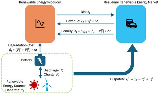
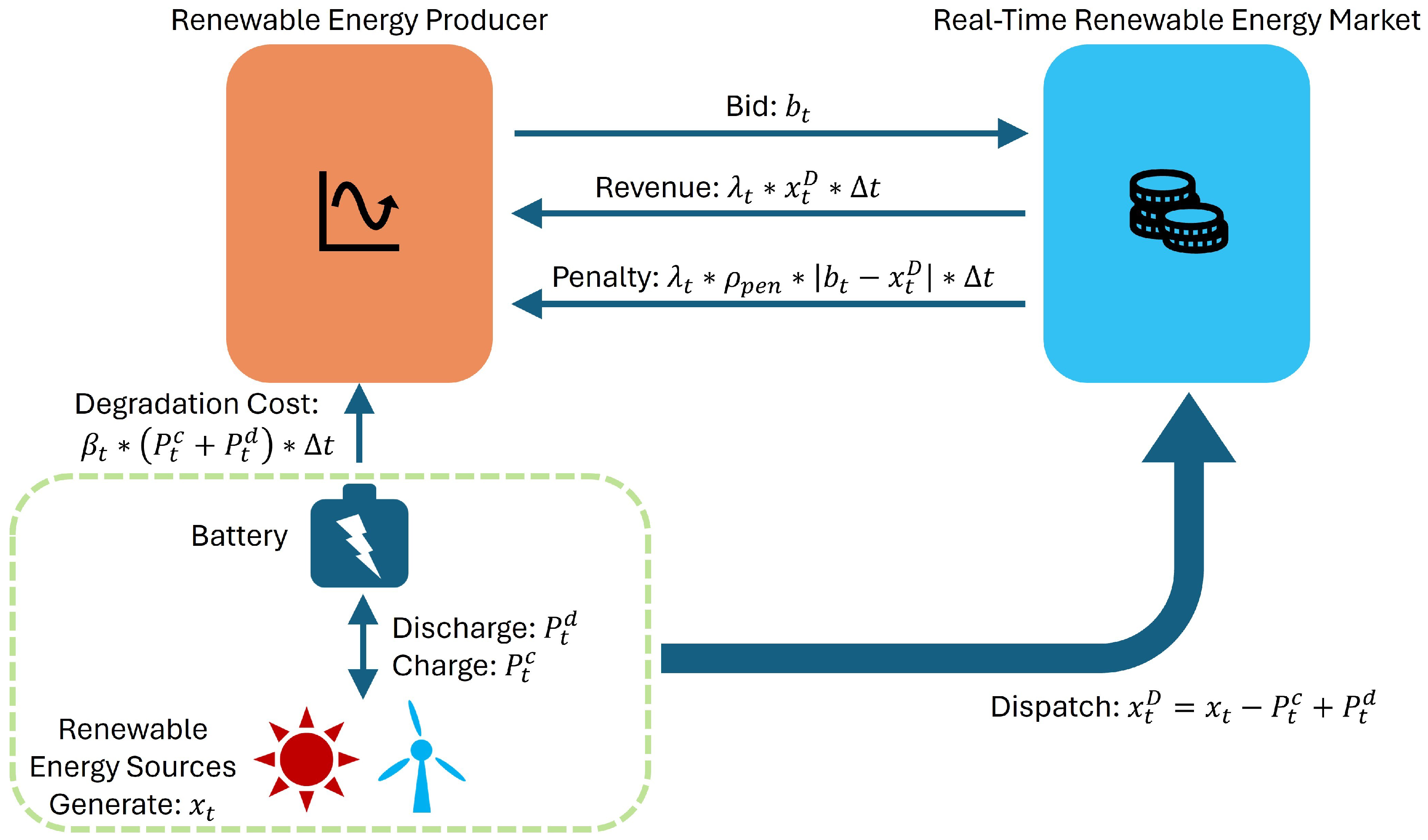
The real-time renewable energy market procedure is shown in Figure 1. It includes the real-time renewable energy market and renewable energy producers equipped with batteries. The profit at any given time slot t is determined by the revenue from real-time renewable energy prices, deviation penalties, and battery degradation costs. Furthermore, the following assumptions are made [1]:

Figure 1. The procedure of the renewable energy market. The diagram illustrates the interactions between renewable energy producers equipped with batteries and the market. It shows how bidding values, actual generation, and battery charge/discharge operations jointly determine dispatch power, profits, and penalties, forming the dynamic decision loop in this paper.

• Price taker assumption: Producers are assumed to be price takers in the real-time renewable energy market. The prices are statistically independent of the bidding values and renewable energy outputs.
• Deviation penalty policy: Deviation penalty exemptions are not allowed. All bidding errors incur deviation penalties, which are critical for maintaining the security and fairness of market operations.
• Bidding gate closure: The closing time is assumed to be near real-time, allowing for more accurate schedules in the real-time market. Clearing prices are calculated for each time slot, such as every 15 min.
• Battery usage: Batteries are considered affordable in the real-time renewable energy market due to rising energy prices, decreasing battery costs, and so on.

2.3. Market Model and Battery Model

At the previous time slot $t-1$, the producer submits a bid $b_t$, a commitment to deliver a specified amount of energy $b_t$ at the next time slot t. The actual renewable energy generation at time slot t is denoted by $x_t$. Moreover, $P_t^c$ and $P_t^d$ are the charging and discharging power at time slot t, respectively. Hence, the dispatch power to the market at time slot t can be given by:

$$x_t^D=x_t-P_t^c+P_t^d.$$

(3)

Next, on the basis of Equation (3), the profit at time slot t, denoted by $f_t$, can be defined as follows:

$$f_t=\{{\lambda }_t(x_t^D-{\rho }_{pen}|b_t-x_t^D|)-{\beta }_t(P_t^c+P_t^d)\}\Delta t,$$

(4)

where ${\lambda }_t$ is the real-time market price at time slot t, ${\rho }_{pen}$ the penalty factor representing the ratio of the deviation penalty to the market price, ${\beta }_t$ the battery degradation cost at time slot t, and $\Delta t$ the duration of the time slot. More specifically, ${\lambda }_t$ per unit of delivered energy is paid to the producer, while ${\lambda }_t\ast {\rho }_{pen}$ per unit of deviated energy is imposed as the deviation penalty. Generally, ${\beta }_t$ depends on the SoC of the battery and is much lower than ${\lambda }_t$. This means the battery degradation cost is significantly lower than the deviation penalty. In summary, we aim to maximize the producer’s profit in the real-time market.

On the other hand, not all charging power can be stored in the battery, nor can all discharging power be dispatched to the market, due to the charging efficiency ${\eta }_t^c$ and discharging efficiency ${\eta }_t^d$. These efficiencies are nonlinear functions of the SoC, depending on the charging power $P_t^c$ and the discharging power $P_t^d$. To calculate them, a steady-state equivalent electrical circuit of the lithium-ion battery cell is used [28]. It is considered while determining the charging or discharging action and value. Nevertheless, the current charging or discharging decisions also impact the SoC in the next time slot. Therefore, decisions should be made to avoid unfavorable states in the next time slot while maximizing profits in the current time slot. For instance, $So{C}_{max}$ and $So{C}_{min}$ are unfavorable states because they limit the ability to under- or over-bid. To address this, our method is based on DRL and is designed to maximize profits over the entire time scale, not just the current period.

3. Our Method

3.1. Our DRL Framework

To accumulate profit $f_t$ over all time slots, we need to address two primary challenges:

• Uncertainties in renewable energy generation and market price: The renewable energy generation $x_t$ and the real-time energy market price ${\lambda }_t$ are not known in advance. Although some traditional distributions can model them, their highly uncertain nature makes it difficult to rely on specific distribution assumptions.
• Time-coupling and sequential decision-making strategy: We cannot consider each time slot separately due to the time-coupling effects. The current charging or discharging decision affects the battery’s SoC, necessitating a sequential decision-making strategy.

Firstly, a DNN can process raw data for the former without requiring definite distributions for $x_t$ and ${\lambda }_t$. Next, for the latter, RL can facilitate interactions between an agent and its environment, allowing us to handle time-coupling in the SoC’s characteristics appropriately. Accordingly, DRL combines the strengths of DNN and RL to address this renewable energy bidding and battery control issue. It is a sequential decision-making strategy, consisting of a set of states S and a set of actions A. At each time slot t, the agent takes action $a_t\in A$ in the state $s_t\in S$ and then transits to the next state $s_{t+1}\in S$, receiving a reward $r_t$. The purpose of DRL is to maximize the cumulative reward, considering a discount factor $\gamma$.

In this issue, the decisions are the bidding value $b_t$, the charging power $P_t^c$, and the discharging power $P_t^d$. For error compensation, excess power $x_t-b_t$ is stored in the battery while $x_t>b_t$, and power deficit $b_t-x_t$ is drawn from the battery while $b_t>x_t$. Additionally, for energy arbitrage, the charging or discharging power can be adjusted by the scaling factor ${\rho }_t$ based on the price ${\lambda }_t$: more power is charged while ${\lambda }_t$ is low, and more power is discharged while ${\lambda }_t$ is high. Here, ${\overline{P}}_t^c$ and ${\overline{P}}_t^d$ denote the upper bounds of the charging and discharging power, respectively. This framework defines the agent’s actions:

$$a_t=(b_t,{\rho }_t),$$

(5)

$$P_t^c=min(max({\rho }_t\ast (x_t-b_t),0),{\overline{P}}_t^c),$$

(6)

$$P_t^d=min(max({\rho }_t\ast (b_t-x_t),0),{\overline{P}}_t^d).$$

(7)

Then, $x_t$, ${\lambda }_t$, and $So{C}_t$ are determined by the environment and define the state $s_t$. Since $x_t$ and ${\lambda }_t$ are unknown while deciding the action $a_t$, we use the observation $o_t=(x_{t-1},{\lambda }_{t-1},So{C}_t)$, and the state is formed with the past observations:

$$s_t=(o_0,o_1,o_2,\dots ,o_{t-2},o_{t-1},o_t).$$

(8)

The reward $r_t$ can be $f_t$ based on our objective. Nevertheless, since $f_t$ includes $x_t$ and ${\lambda }_t$, both of which are beyond the agent’s control, it will induce noise into the reward function and complicate the training procedure. Thus, we define the reward function based on the profit difference compared to perfect forecast bidding without the use of a battery, and the reward function is formulated:

$$r_t=f_t-{\lambda }_t\ast x_t\ast \Delta t.$$

(9)

Since $x_t$ and ${\lambda }_t$ are obtained independently of $a_t$, $r_t$ increases monotonically with regard to $f_t$. It means that maximizing $r_t$ is equivalent to maximizing $f_t$. Hence, we can reduce variance in the learning process by minimizing randomness in the reward signal while still achieving maximum total profit. Notably, we do not require explicit forecasting of the real-time price; it is implicitly included in the reward.

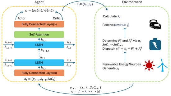
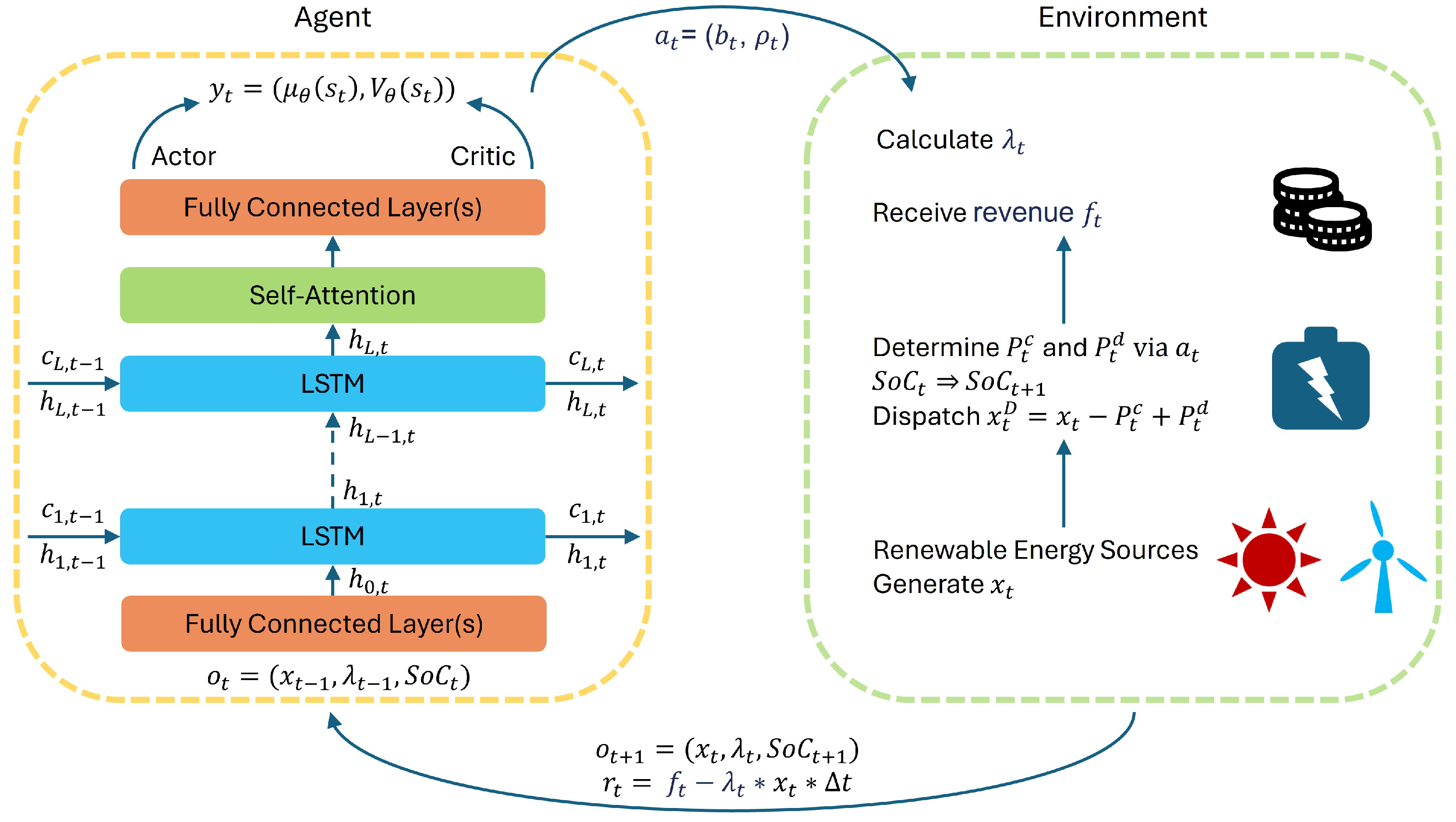
The overall framework is illustrated in Figure 2. The renewable energy producer acts as an RL agent, interacting with the RL environment by sending various actions. The RL environment consists of the real-time energy market, renewable energy source(s), and a battery, which will return a reward and the new observation to the RL agent. The agent learns the policy until it can find actions for all states that maximize the total cumulative reward. In the framework, the state $s_t$ serves as input to the DNN, which serves as the agent’s thinking mechanism. In the thinking mechanism, LSTM is adopted due to its ability to handle time-series observations. It is also extensively employed to predict renewable energy generation and market prices, demonstrating superior performance compared to conventional networks [1]. Consider that there are L hidden layers in the LSTM block, and at each hidden layer l and time slot t, $c_{l,t}$ and $h_{l,t}$ represent a cell state vector and a hidden output vector, respectively. Then, with the input vectors $o_t=(x_{t-1},{\lambda }_{t-1},So{C}_t)$ and the output vector $y_t$, the complete relationships in the LSTM block are described by

$$h_{0,t}=ReLU(W_i{o}_t+b_i),$$

(10)

$$(c_{l,t},h_{l,t})=LSTM(c_{l,t-1},h_{l,t-1},h_{l-1,t}),$$

(11)

$$y_t=W_o{h}_{L,t}+b_o,$$

(12)

where $W_i$ and $W_o$ are weight matrices, $b_i$ and $b_o$ are bias vectors, $ReLU\left(z\right)=max(z,0)$ is a rectified linear unit activation function, and $LSTM\left(\right)$ is the standard LSTM function. Since $c_{l,t-1}$ and $h_{l,t-1}$ include the preceding observations, we can get the state $s_t=(H_{t-1},o_t)$, where $H_{t-1}$ expresses $c_{l,t-1}$ and $h_{l,t-1}$ for all layers. Henceforth, all weight matrices and bias vectors will be collectively referred to as the parameter $\theta$.

Figure 2. Architecture of the DRL framework. The illustration depicts how the RL agent interacts with the environment (renewable source, battery, and market). The agent receives observations, outputs bidding and control actions, and updates its policy to maximize long-term profits.

Although LSTM captures sequential dependencies, information dilution over long sequences weakens its sensitivity to non-adjacent but decision-critical patterns, e.g., recurring price peaks, irregular SoC thresholds, and so on. The attention mechanism addresses this limitation by dynamically weighting all time steps, enabling selective focus on the most relevant historical observations. Hence, LSTM and attention are complementary rather than redundant, and the concept of self-attention is applied following the LSTM blocks. It can be described mathematically using the following equations. Let X be the input sequence, and $X\leftarrow h_{L,t}$ is adopted in our framework. For each input $x_i$, we compute Query(Q), Key(K), and Value(V) as follows:

$$Q=X{W}_Q,$$

(13)

$$K=X{W}_K,$$

(14)

$$V=X{W}_V,$$

(15)

where $W_Q$, $W_K$, and $W_V$ are learned weight matrices. The attention scores are computed as the dot product of Q and K to obtain the similarity scores, and are then scaled by $1/\sqrt{d_k}$ to prevent large values. Then, they are passed through the softmax activation function to obtain the attention weights. Finally, the output is obtained by multiplying the attention weights by V.

$$Attention(Q,K,V)=softmax({\displaystyle \frac{Q{K}^T}{\sqrt{d_k}}})V.$$

(16)

3.2. PPO Algorithm

Given the continuous nature of actions, we adopt an actor–critic policy gradient method to achieve continuous control. The actor parameterizes the RL policy as ${\pi }_{\theta }\left(a_t\right|s_t)$, representing the probability density of taking action $a_t$ in state $s_t$ with parameter $\theta$. Specifically, ${\pi }_{\theta }\left(a_t\right|s_t)$ is modeled as a multivariate Gaussian distribution, where the actor outputs the mean vector ${\mu }_{\theta }\left(s_t\right)$ and covariance matrix ${\sigma }^{2}I$ (with identity matrix I), and the critic estimates the value function $V_{\theta }\left(s_t\right)$. During training, $a_t$ is sampled from ${\pi }_{\theta }\left(a_t\right|s_t)$, while during testing, $a_t$ is set to ${\mu }_{\theta }\left(s_t\right)$. Since specific parameters, such as the deviation penalty factor and battery degradation cost, may change across different scenarios and necessitate retraining, an efficient DRL algorithm with straightforward implementation and strong continuous control performance is essential. Therefore, we adopt PPO, which learns the optimal policy from the state–value function and allows parameter sharing between the actor and critic. Given that the inputs consist solely of states, PPO enables fast learning, and the outputs naturally encompass both the policy and value function as $y_t=({\mu }_{\theta }\left(s_t\right),V_{\theta }\left(s_t\right))$.

The goal of PPO is to constrain policy updates to prevent overfitting to the latest batch of data. Namely, PPO aims to ensure that the updated parameter, $\theta$, does not significantly deviate from the previous one, ${\theta }_{old}$. The agent empirically executes the policy ${\pi }_{{\theta }_{old}}$ for T steps to collect $(s_0,a_0,r_0,s_1,a_1,r_1,\dots ,s_{T-1},a_{T-1},r_{T-1},s_T)$. Subsequently, the PPO actor employs the clipped surrogate objective:

$${\mathcal{L}}_{\pi }^{clip}\left(\theta \right)={\displaystyle \frac{1}{T}}\sum min\left({\displaystyle \frac{{\pi }_{\theta }\left(a_t\right|s_t)}{{\pi }_{{\theta }_{old}}\left(a_t\right|s_t)}}{\widehat{A}}_t,g(ϵ,{\widehat{A}}_t)\right),$$

(17)

$$g(ϵ,{\widehat{A}}_t)=\left\{\begin{array}{c}(1+ϵ){\widehat{A}}_{t}if {\widehat{A}}_t\ge 0,\hfill \\ (1-ϵ){\widehat{A}}_{t}if {\widehat{A}}_t<0,\hfill \end{array}\right.$$

(18)

where ${\widehat{A}}_t$ is an estimate of the advantage function and $ϵ$ a hyperparameter. By clipping the ratio at $1+ϵ$ or $1-ϵ$, the latter ensures that the updated $\theta$ does not significantly deviate from the previous ${\theta }_{old}$. Then, the PPO critic employs the Mean Squared Error (MSE) concept of estimated value functions:

$${\mathcal{L}}_V\left(\theta \right)={\displaystyle \frac{1}{T}}\sum {(V_t^{targ}-V_{\theta }\left(s_t\right))}^2,$$

(19)

where $V_t^{targ}=r_t+\gamma V_{\theta }\left(s_{t+1}\right)$, and it is used for each update of constant values.

Next, ${\widehat{A}}_t$, the advantage function, indicates the relative quality of an action compared to other available actions. Since this method is biased due to relying on the estimated value function of the critic, PPO employs Generalized Advantage Estimation (GAE) to evaluate ${\widehat{A}}_t$, reducing variance significantly while maintaining an acceptable level of bias:

$${\widehat{A}}_t=\sum {(\gamma \Lambda )}^k{\widehat{\delta }}_{t+k},$$

(20)

where ${\widehat{\delta }}_t=r_t+\gamma V_{\theta }\left(s_{t+1}\right)-V_{\theta }\left(s_t\right)$ is the temporal difference error, and $\Lambda \in (0,1)$ controls the trade-off between bias and variance.

Finally, according to the discussions above, we can obtain the objective, minimized at every iteration. Note that the entropy bonus is omitted for simplicity, as the exploration is driven by the stochastic policy ${\pi }_{\theta }\left(a_t\right|s_t)$:

$$\mathcal{L}\left(\theta \right)=-{\mathcal{L}}_{\pi }^{clip}\left(\theta \right)+K{\mathcal{L}}_V\left(\theta \right),$$

(21)

where the coefficient K is used for the critic learning. At every iteration, the agent collects $(s_0,a_0,r_0,\dots ,s_{T-1},a_{T-1},r_{T-1},s_T)$ in accordance with the policy ${\pi }_{{\theta }_{old}}$. $\mathcal{L}\left(\theta \right)$ is then minimized utilizing the collected data for K epochs with learning rate $\alpha$. Subsequently, T is reset to 0, and ${\theta }_{old}$ is replaced with the updated $\theta$. This procedure is repeated until convergence. During testing, renewable energy producers calculate actions using their trained models at each time slot and send them to the experimental environment. The real-time energy market calculates the final profit to be paid to renewable energy producers based on these actions.

4. Experimental Results

4.1. Experimental Environments and Comparisons

Here, we begin describing the experimental environment. We use 15 min time-series open datasets for solar power, wind power, and real-time energy prices from 2016 to 2019 [1], where the solar data are from the distribution system operator PBE and the wind data are from Elia-connected Wallonie. Both are aggregated from distributed renewable energy sources, helping stabilize output variability. To prevent the parameters in NNs from shrinking, we will normalize all relevant data using Min–Max normalization with respect to the renewable generation capacity $x_{max}$, then denormalize them to obtain valid outputs. This is an ordinary but critical skill for Machine Learning (ML) issues. The mean value of the real-time energy price $p_{mean}$ is $50/MWh, with prices calculated every 15 min, making $\Delta t=0.25$ h. We exclude nighttime data (zero values) from the solar power datasets. All datasets are split into a training set (50%: 2016 and 2017), a validation set (25%: 2018), and a test set (25%: 2019). This chronological split is intentional, rather than a random partitioning, to preserve the temporal order of the data and prevent look-ahead bias, ensuring that the model is always evaluated on unseen future data.

Next, the battery capacity is typically set to a size comparable to the renewable generation capacity in the day-ahead market. Due to the high cost of batteries, such a size would be expensive and impractical. Hence, $P_{max}$ and $E_{max}$ are set to $0.15\ast x_{max}$ in this paper. It might still seem high given the battery costs, but using a smaller battery would result in lower profit due to reduced utilization. Assuming investment incentives and tax credits from subsidy programs, a battery size of 15% of $x_{max}$ becomes affordable. At the first time step of each RL procedure, $So{C}_0$ is initialized to 0.5. Furthermore, all parameters related to the experiments are summarized in Table 1, including battery, market, PPO, and DNN settings. Notably, the authors in [1] do not discuss the possibility of further improving performance by adjusting hyperparameters. It motivates us to begin the first part of this research, namely, to provide more feasible settings for the critical parameters to improve the training and testing procedures. More specifically, to ensure a fair and consistent comparison with prior research, all battery and market parameters are identical to those used in the baseline study. Regarding the PPO and DNN settings, several hyperparameters are fine-tuned to achieve stable convergence and high cumulative profit. The learning rate is selected to balance convergence speed and policy stability. Larger values lead to divergence, whereas smaller ones slow convergence. The number of hidden neurons determines the model’s capacity and memory depth. The ablation study demonstrates the best trade-off between computational efficiency and performance robustness. The episode length controls the temporal horizon of decision-making. Longer episodes improve long-term reward capture but increase variance, so multiple configurations are evaluated for robustness.

Table 1. Experimental parameters.

Battery and Market Settings	Value
ine Time slot $\Delta t$	0.25 h
Renewable generation capacity $x_{max}$	100 MW
Mean energy price $p_{mean}$	$50/MWh
Max battery power $P_{max}$	15 MW
Battery capacity $E_{max}$	15 MWh
Deviation penalty factor ${\rho }_{pen}$	1
Minimum SoC $So{C}_{min}$	0.1
Maximum SoC $So{C}_{max}$	0.9
Degradation cost $\beta$	$10/MWh
The number of battery cells $N_{cell}$	130 × 215 × 150
ine PPO and DNN settings	Value
ine The number of Self-Attention components	1
Hidden dimension of Self-Attention	32
The number of heads of Self-Attention	4
The number of LSTM components	2
The number of hidden neurons U	32, 64 & 128
Optimizer	Adam
Learning rate $\alpha$	0.001
The number of time steps in episode T	64, 128, 512, 1024 & 2048
The number of epochs per episode K	3
Discount factor $\gamma$	0.99, 0.90 & 0.81
Controlled parameter in GAE $\Lambda$	0.95
Clipping parameter in PPO $ϵ$	0.01
Coefficient of the critic learning $\kappa$	1
Standard deviation of the policy $\sigma$	0.1

The discount factor is tuned to assess sensitivity to future reward weighting, while the clipping parameter ensures smooth, stable policy updates within PPO. The GAE parameter provides a well-established balance between bias and variance in advantage estimation. The critic learning coefficient maintains balance in actor–critic training, preventing overemphasizing policy or value loss. The policy standard deviation introduces controlled exploration noise. Smaller reduces diversity, while larger increases volatility.

The Adam optimizer is employed for its proven stability in deep reinforcement learning applications, and the number of epochs is empirically set to ensure convergence without overfitting recent experiences. Finally, the model integrates two LSTM layers and one self-attention layer to enhance temporal and contextual feature extraction. This configuration has been validated through ablation experiments, confirming its effectiveness in maximizing cumulative profit while preserving training stability.

The specification of our experimental computer is shown below:

• Computer model: Mac Studio
• Chipset: Apple M2 Max
• RAM: 96 GB
• OS: MacOS Sonoma 14.5
• Machine learning library: PyTorch 2.4.0 [29].

On the other hand, in [1], the authors compare their research with several studies. However, direct comparisons with those studies would be inappropriate or misleading, since they are based on different experimental conditions, e.g., comparing with that in [30] without utilizing batteries, comparing with that in [7] without considering the concept of error compensation, and comparing with those in [2,3,19] without adopting the idea of energy arbitrage. Based on their experiments, ref. [1] achieves the best performance among all compared methods. Therefore, we will only compare with [1], as we both operate under the same conditions: batteries, error compensation, and energy arbitrage.

4.2. Performance Evaluation

Table 1 summarizes the PPO and DNN settings in the performance evaluation. As shown, selecting appropriate hyperparameters is challenging due to the numerous options available. Consequently, we draw on [1] for the hyperparameters and further tune them based on our experience to achieve better performance. More specifically, we further consider:

• The number of hidden neurons U: Determining the capacity for the network to learn, store, and utilize information effectively and ultimately impacting the overall performance of the model.
• The number of time steps in episode T: Balancing capturing adequate context and maintaining computational efficiency.
• Discount factor $\gamma$: Determining how much the future states influence the current action selections.

Moreover, this research adopts the self-attention component in DRL, which enhances the ability to process and interpret sequences of observations or actions by focusing on the most relevant parts of the input data. Here, the input data is the output data of the LSTM components above in our architecture. As reported in Table 1, the self-attention module is configured with a hidden dimension of 32 and 4 attention heads.

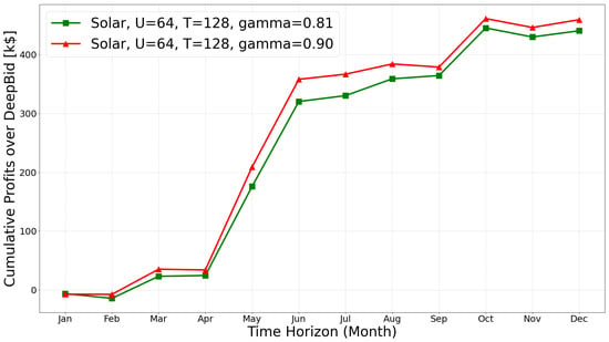
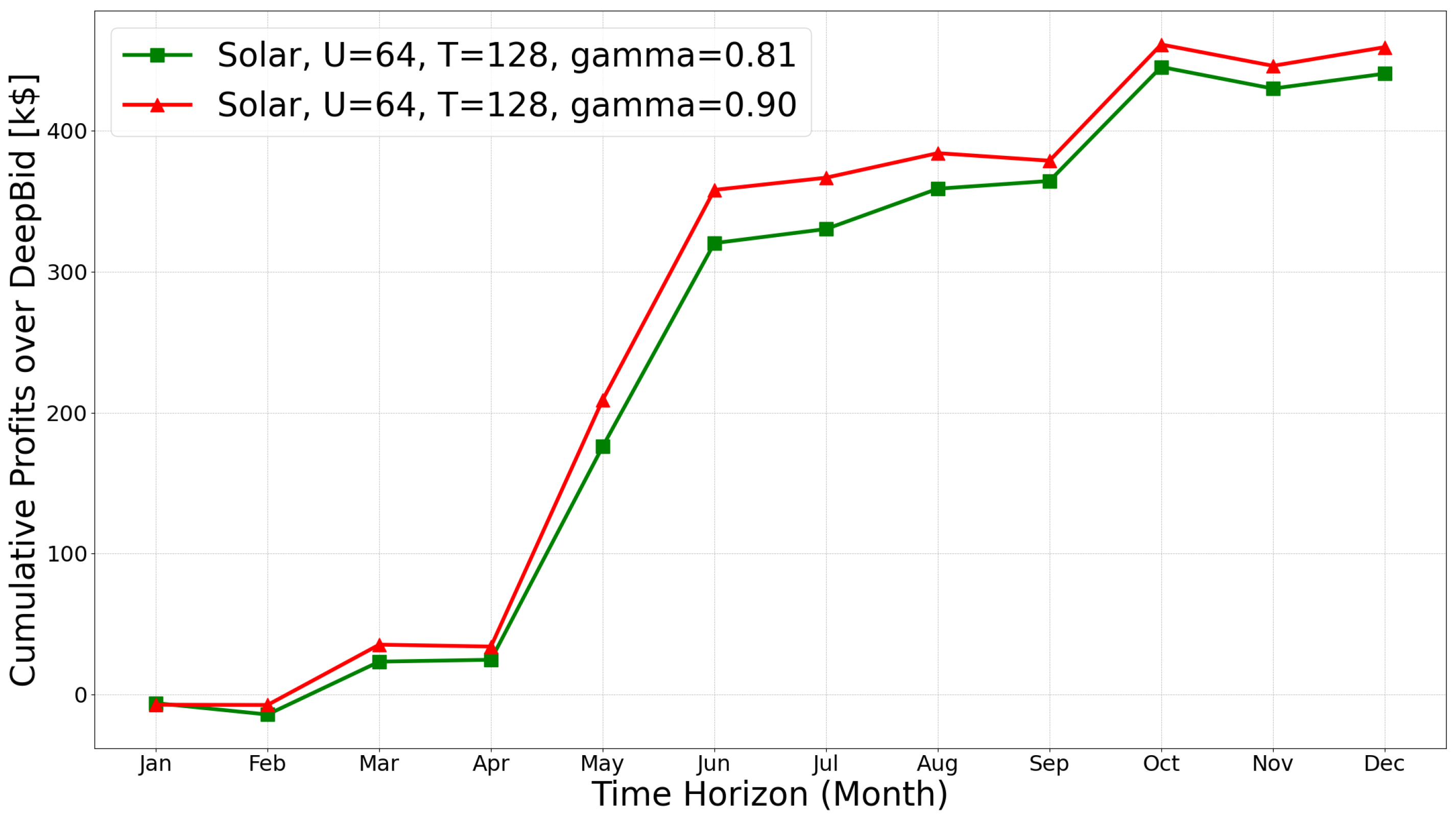
Here, we start to illustrate the experimental results. The method proposed in [1] is called DeepBid and will be used in all subsequent discussions for simplicity. Note that although we conduct many experiments, not every setting performs well. Therefore, we will only present the best experimental results, focusing on them to simplify the figures and descriptions. Figure 3 represents a comparison of cumulative profits over DeepBid over a 12-month time horizon for two different scenarios involving solar energy, identified by various parameters (the model with $U=64$, $T=128$, and $\gamma =0.81$ and the model with $U=64$, $T=128$, and $\gamma =0.90$). In this figure, the x-axis represents the time horizon from January to December. The y-axis shows the cumulative profits over DeepBid, expressed in thousands of dollars. Remarkably, the better one, marked by red triangles, starts to diverge from the one marked by green squares around April and shows a more aggressive increase in profits, especially from May to June. Although both lines follow a similar trend, the red line consistently remains above the green line, indicating higher cumulative earnings throughout the year. This figure shows that a model with specific U, T, and $\gamma$ may lead to more aggressive, long-term strategies that yield higher profits in the context of solar power.

Figure 3. Comparison of cumulative profits relative to DeepBid for solar power data. The time-series plot shows cumulative earnings over 12 months, demonstrating that the models with various configurations consistently yield higher profits than the baseline.

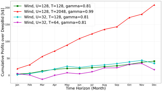
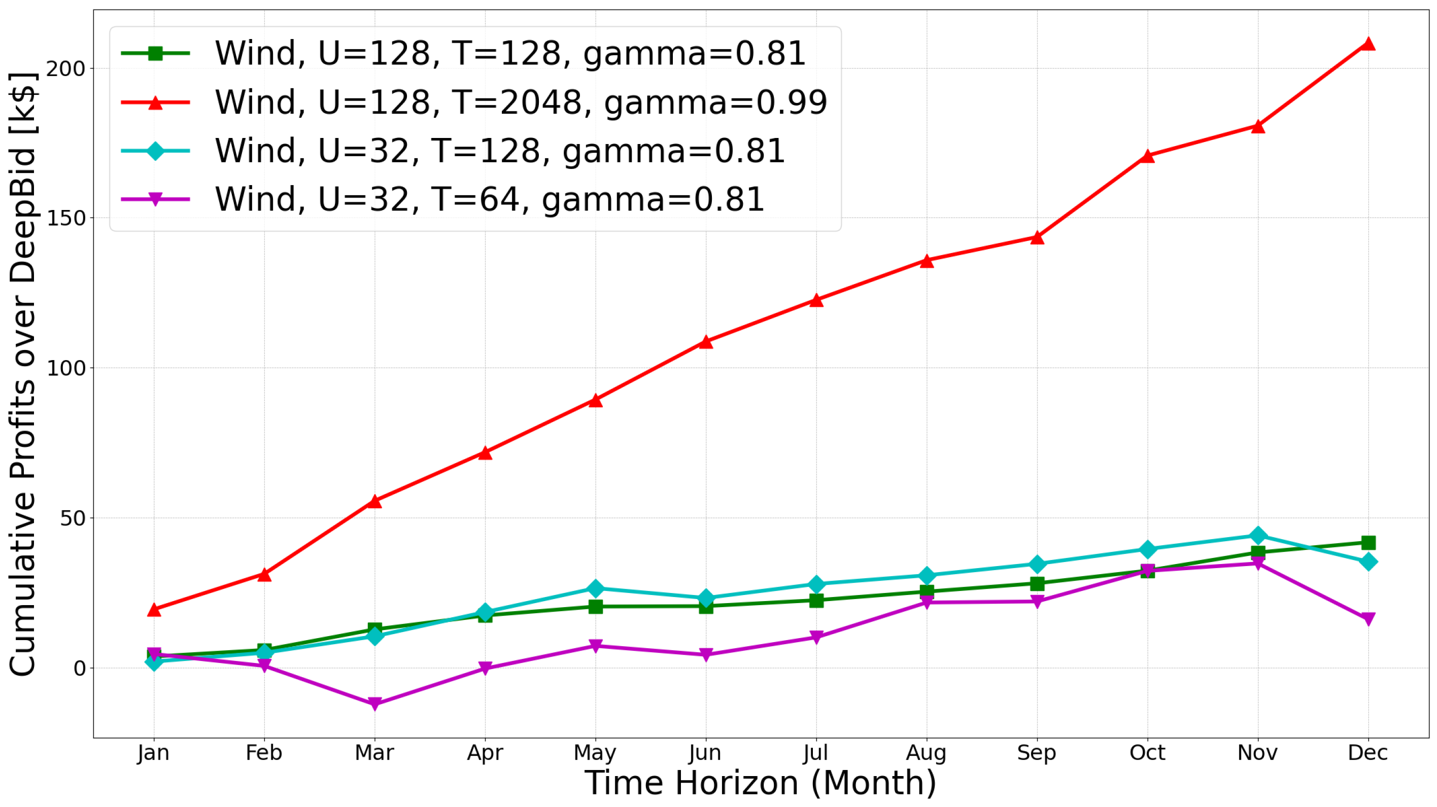
Figure 4 illustrates the cumulative profits over DeepBid over a 12-month time horizon for four different scenarios involving wind energy, identified by various parameters (the model with $U=128$, $T=128$, and $\gamma =0.81$, the model with $U=128$, $T=2048$, and $\gamma =0.99$, the model with $U=32$, $T=128$, and $\gamma =0.81$, and the model with $U=32$, $T=64$, and $\gamma =0.81$). The definitions of the x-axis and y-axis are the same as in Figure 3. In this figure, the better-performing one, marked by red triangles, shows a significant and consistent increase in cumulative profits, especially after February. By the end of the year, it also has the highest cumulative profits among all models. The figure shows that, in the context of wind power, larger U, larger T, and higher $\gamma$ significantly boost cumulative profits (i.e., the red line). Smaller parameters result in much lower cumulative profits. Notably, the purple line performs the worst. Its cumulative profit for the entire year is only slightly above DeepBid’s and is even lower than DeepBid’s in the early months.

Figure 4. Comparison of cumulative profits relative to DeepBid for wind power data. The time-series plot shows cumulative earnings over 12 months, demonstrating that the models with various configurations consistently yield higher profits than the baseline.

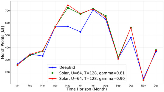
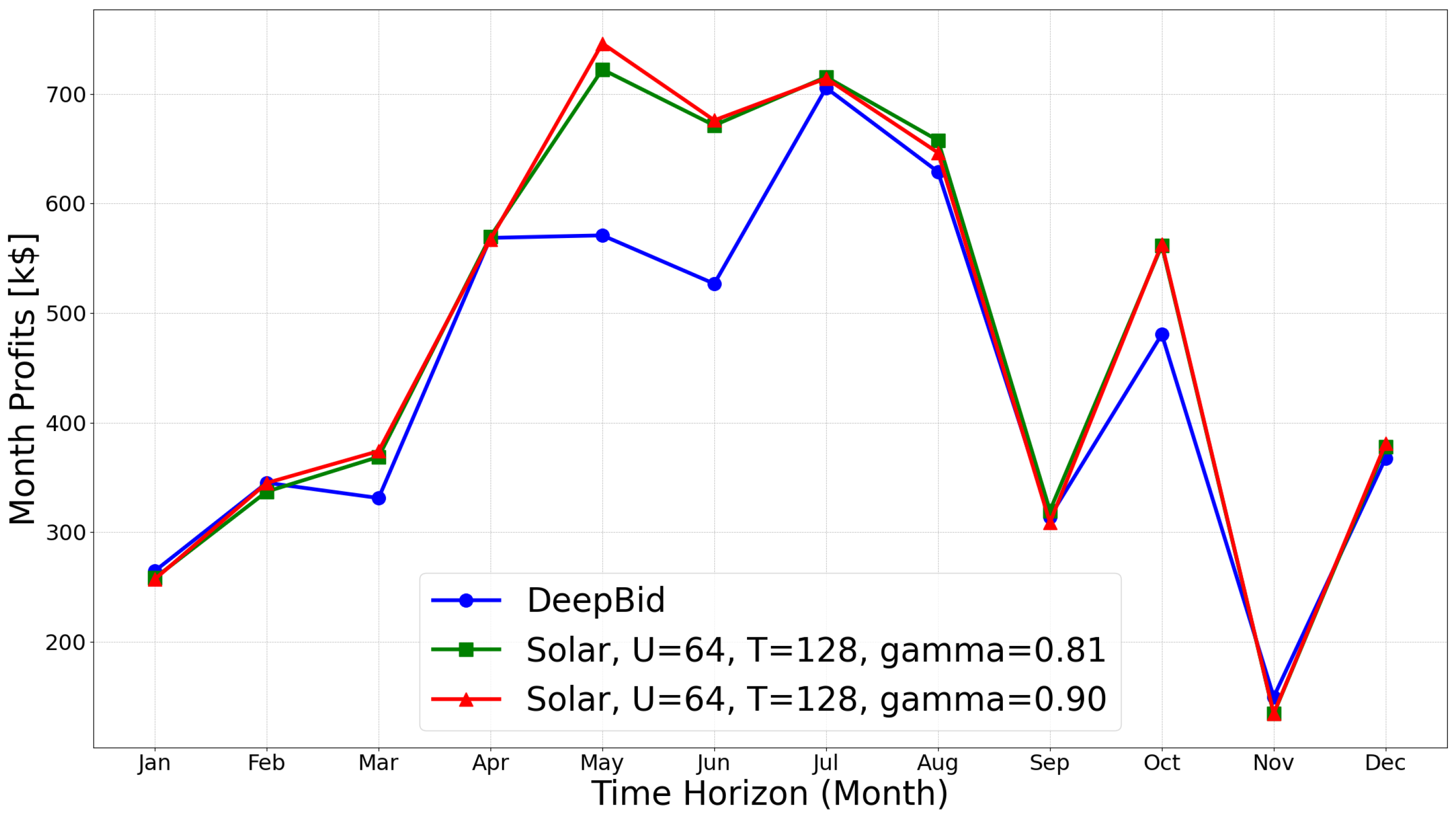
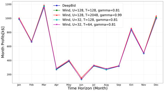
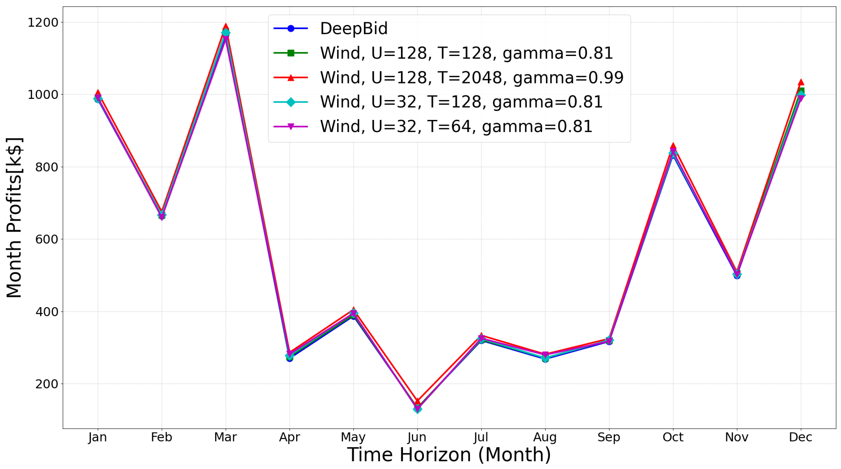
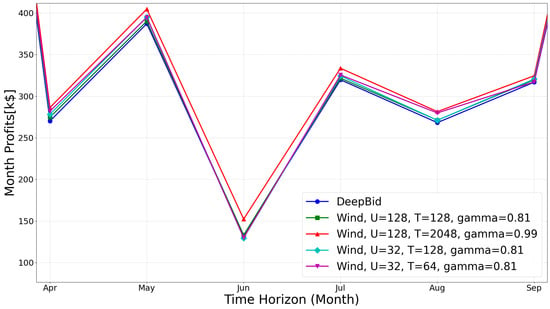
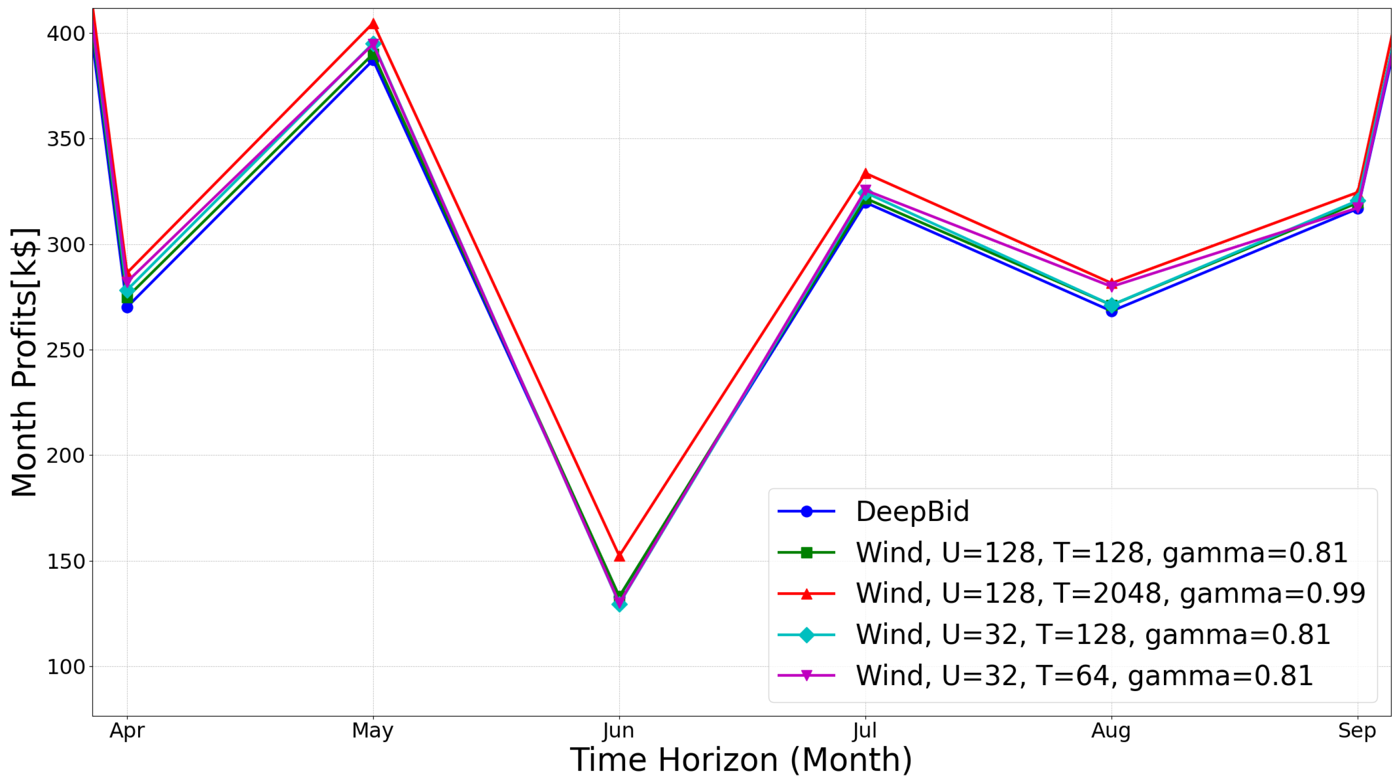
Figure 5 illustrates the monthly profits related to solar energy over a 12-month time horizon, including a comparison with DeepBid. Here, the x-axis represents the time horizon in months, and the y-axis shows the monthly profits in thousands of dollars. Initially, all perform similarly, with minimal differences in monthly profits. Then, in the middle of the year, both our methods consistently outperform DeepBid. Finally, a significant profit drop occurs later in the year, with DeepBid taking the biggest hit. This figure shows that our method with $U=64$, $T=128$, and $\gamma =0.90$ consistently outperforms DeepBid regarding monthly profits. It is more robust, maintaining higher profits throughout most of the year, particularly in months with significant performance fluctuations. Figure 6 displays the monthly profits related to wind energy over a 12-month time horizon, including a comparison with DeepBid. The definitions of the x-axis and y-axis are the same as in Figure 5. All models follow almost identical profit trends throughout the year. Here, we zoom in on the results for specific months in Figure 7, where the model with $U=128$, $T=2048$, and $\gamma =0.99$ tends to outperform the others, particularly in April, May, and September. It consistently leads in monthly profits, although the margin is narrow.

Figure 5. Monthly profit comparison for solar power data between the proposed model and DeepBid. The plot highlights that our approach achieves higher yearly profits, particularly in mid-year months.

Figure 6. Monthly profit comparison for wind power data between the proposed model and DeepBid. The curves maintain a consistent advantage over DeepBid.

Figure 7. Zoomed-in view of selected months from Figure 6 for wind power data. The results clarify the profit margin differences, showing that the configuration $U=128$, $T=2048$, and $\gamma =0.99$ consistently outperforms other models.

The results show improvements for renewable energy producers, yielding cumulative gains exceeding 400 k and 200 k for solar and wind, respectively. To further validate the stability of the proposed framework, we conduct 30 independent runs with different random seeds. The results deliver mean cumulative profits of 430 k ($\sigma$ = 118.71 k) for solar energy and 204 k ($\sigma$ = 13.38 k) for wind energy, confirming that the observed performance gains are consistent and are not attributable to stochastic variance in the training process. Moreover, the more pronounced improvement in solar energy (approximately 7.9%) compared to wind (approximately 2.8%) reflects the distinct variability and predictability characteristics of each generation type. To further enhance both the stability of solar energy and the performance of wind energy, integrating weather prediction models into the RL framework could provide richer contextual signals, enabling the agent to anticipate generation variability better and adapt bidding strategies accordingly.

From a market risk management perspective, the bidding-and-control framework reduces exposure to forecast uncertainty and real-time price volatility. The RL agent dynamically refines bidding decisions by capturing temporal dependencies through attention mechanisms, minimizing deviation penalties, and stabilizing revenues. Regarding battery utilization, the joint optimization of bidding and SoC management enables intelligent scheduling of charging and discharging activities. Batteries are transformed from passive storage devices into active market participants that hedge against volatility, absorb surplus generation, exploit price arbitrage opportunities, and avoid excessive degradation.

Finally, regarding the computational efficiency of the proposed model, we measure the inference time on our experimental computer (Mac Studio with Apple M2 Max and 96 GB RAM). Over a total of 34,889 inference steps, the cumulative inference time is 4.1871 s, delivering an average inference latency of approximately 0.00012 s per step. Since the inputs consist solely of numerical time-series data, the model introduces negligible computational overhead. These results confirm that the proposed framework is well-suited for near-real-time market deployment and that computational complexity is not a practical concern in this context.

5. Conclusions

In this study, we present an attention-enhanced long short-term memory reinforcement learning framework for renewable energy bidding and battery control. The proposed method achieves substantial performance gains over existing strategies, producing cumulative profits of over 400 k for solar energy and more than 200 k for wind energy. These results highlight the superior ability to balance real-time bidding precision and battery utilization efficiency, leading to higher overall profitability and stability in renewable energy market participation.

Next, future research may further investigate how the proposed approach can assist renewable energy producers in optimizing bidding strategies and battery operations, and validate its scalability across larger, more complex real-world power systems. Future work will also conduct sensitivity analyses under varying penalty factors, battery degradation costs, and price volatility levels to validate its robustness across diverse market conditions.

References

- Jeong, J.; Kim, S.W.; Kim, H. Deep reinforcement learning based real-time renewable energy bidding with battery control. IEEE Trans. Energy Mark. Policy Regul. 2023, 1, 56–96. [Google Scholar] [CrossRef] [Scilit]
- Bae, K.Y.; Jang, H.S.; Jung, B.C.; Sung, D.K. Effect of prediction error of machine learning schemes on photovoltaic power trading based on energy storage systems. Energies 2019, 12, 1249. [Google Scholar] [CrossRef] [Scilit]
- Gholami, M.; Fathi, S.H.; Milimonfared, J.; Chen, Z.; Deng, F. A new strategy based on hybrid battery—Wind power system for wind power dispatching. IET Gener. Transm. Distrib. 2018, 12, 160–169. [Google Scholar] [CrossRef]
- Yang, J.; Yang, M.; Wang, M.; Du, P.; Yu, Y. A deep reinforcement learning method for managing wind farm uncertainties through energy storage system control and external reserve purchasing. Int. J. Electr. Power Energy Syst. 2020, 119, 105928. [Google Scholar] [CrossRef] [Scilit]
- Huang, B.; Wang, J. Deep-reinforcement-learning-based capacity scheduling for PV-battery storage system. IEEE Trans. Smart Grid 2020, 12, 2272–2283. [Google Scholar] [CrossRef] [Scilit]
- Harrold, D.J.; Cao, J.; Fan, Z. Data-driven battery operation for energy arbitrage using rainbow deep reinforcement learning. Energy 2022, 238, 121958. [Google Scholar] [CrossRef] [Scilit]
- Xie, Y.; Guo, W.; Wu, Q.; Wang, K. Robust MPC-based bidding strategy for wind storage systems in real-time energy and regulation markets. Int. J. Electr. Power Energy Syst. 2021, 124, 106361. [Google Scholar] [CrossRef] [Scilit]
- Mohy-ud-din, G.; Muttaqi, K.M.; Sutanto, D. A cooperative energy transaction model for VPP integrated renewable energy hubs in deregulated electricity markets. IEEE Trans. Ind. Appl. 2022, 58, 7776–7791. [Google Scholar] [CrossRef] [Scilit]
- Nezamabadi, H.; Vahidinasab, V. Market bidding strategy of the microgrids considering demand response and energy storage potential flexibilities. IET Gener. Transm. Distrib. 2019, 13, 1346–1357. [Google Scholar] [CrossRef] [Scilit]
- Aguiar, N.; Gupta, V. An insurance contract design to boost storage participation in the electricity market. IEEE Trans. Sustain. Energy 2021, 12, 543–552. [Google Scholar] [CrossRef] [Scilit]
- Nezamabadi, H.; Vahidinasab, V. Arbitrage strategy of renewable-based microgrids via peer-to-peer energy-trading. IEEE Trans. Sustain. Energy 2021, 12, 1372–1382. [Google Scholar] [CrossRef] [Scilit]
- Liu, J.; Ma, Y.; Chen, Y.; Zhao, C.; Meng, X.; Wu, J. Multi-agent deep reinforcement learning-based cooperative energy management for regional integrated energy system incorporating active demand-side management. Energy 2025, 319, 135056. [Google Scholar] [CrossRef] [Scilit]
- Xie, J.; Ajagekar, A.; You, F. Multi-agent attention-based deep reinforcement learning for demand response in grid-responsive buildings. Appl. Energy 2023, 342, 121162. [Google Scholar] [CrossRef] [Scilit]
- Chang, C.-C.; Wang, H.-W.; Zeng, Y.-X.; Huang, J.-D. Using machine learning approaches to improve ultra-wideband positioning. J. Internet Technol. 2021, 22, 1019–1029. [Google Scholar] [CrossRef] [Scilit]
- Hwang, K. Cloud Computing for Machine Learning and Cognitive Applications; The MIT Press: Cambridge, UK, 2017. [Google Scholar]
- Hwang, K.; Chen, M. Big-Data Analytics for Cloud, IoT and Cognitive Computing; Wiley: Hoboken, NJ, USA, 2017. [Google Scholar]
- Sutton, R.S.; Barto, A.G. Reinforcement Learning: An Introduction; The MIT Press: Cambridge, UK, 2018. [Google Scholar]
- Sewak, M. Deep Reinforcement Learning: Frontiers of Artificial Intelligence; Springer: Cham, Switzerland, 2019. [Google Scholar]
- Jeong, J.; Kim, H. Deepcomp: Deep reinforcement learning based renewable energy error compensable forecasting. Appl. Energy 2021, 294, 116970. [Google Scholar] [CrossRef] [Scilit]
- Du, Y.; Li, F.; Zandi, H.; Xue, Y. Approximating nash equilibrium in day-ahead electricity market bidding with multi-agent deep reinforcement learning. J. Mod. Power Syst. Clean Energy 2021, 9, 534–544. [Google Scholar] [CrossRef] [Scilit]
- Cao, J.; Harrold, D.; Fan, Z.; Morstyn, T.; Healey, D.; Li, K. Deep reinforcement learning-based energy storage arbitrage with accurate lithium-ion battery degradation model. IEEE Trans. Smart Grid 2020, 11, 4513–4521. [Google Scholar] [CrossRef] [Scilit]
- Chang, C.-C.; Tsai, J.; Lu, P.-C.; Lai, C.-A. Accuracy improvement of autonomous straight take-off, flying forward, and landing of a drone with deep reinforcement learning. Int. J. Comput. Intell. Syst. 2020, 13, 914–919. [Google Scholar] [CrossRef] [Scilit]
- Chang, C.-C.; Tsai, J.; Lin, J.-H.; Ooi, Y.-M. Autonomous driving control using the DDPG and RDPG algorithms. Appl. Sci. 2021, 11, 10659. [Google Scholar] [CrossRef] [Scilit]
- LSTM—PyTorch 2.3 Documentation. Available online: https://pytorch.org/docs/stable/generated/torch.nn.LSTM.html (accessed on 2 April 2026).
- Vaswani, A.; Shazeer, N.; Parmar, N.; Uszkoreit, J.; Jones, L.; Gomez, A.N.; Kaiser, Ł.; Polosukhin, I. Attention is all you need. In Proceedings of the Advances in Neural Information Processing Systems 30 (NIPS 2017), Long Beach, CA, USA, 4–9 December 2017. [Google Scholar]
- MultiheadAttention—PyTorch 2.3 Documentation. Available online: https://pytorch.org/docs/stable/generated/torch.nn.MultiheadAttention.html (accessed on 2 April 2026).
- Schulman, J.; Wolski, F.; Dhariwal, P.; Radford, A.; Klimov, O. Proximal policy optimization algorithms. arXiv 2017, arXiv:1707.06347v2. [Google Scholar] [CrossRef] [Scilit]
- Chen, M.; Rincon-Mora, G.A. Accurate electrical battery model capable of predicting runtime and I–V performance. IEEE Trans. Energy Convers. 2006, 21, 504–511. [Google Scholar] [CrossRef] [Scilit]
- PyTorch. Available online: https://pytorch.org/ (accessed on 2 April 2026).
- Yang, D.; Wu, E.; Kleissl, J. Operational solar forecasting for the real-time market. Int. J. Forecast. 2019, 35, 1499–1519. [Google Scholar] [CrossRef] [Scilit]
Disclaimer/Publisher’s Note: The statements, opinions and data contained in all publications are solely those of the individual author(s) and contributor(s) and not of MDPI and/or the editor(s). MDPI and/or the editor(s) disclaim responsibility for any injury to people or property resulting from any ideas, methods, instructions or products referred to in the content. |
© 2026 by the authors. Licensee MDPI, Basel, Switzerland. This article is an open access article distributed under the terms and conditions of the Creative Commons Attribution (CC BY) license.