Distribution Network Fault Location Method Based on Limited Measurement Information

Abstract

Due to the complex structure and large number of nodes in distribution networks, it is difficult to achieve full coverage of synchronous phasor measurement units (μPMUs) in actual engineering projects, resulting in limited available measurement data. To address this issue, this paper proposes a distribution network fault location method based on limited measurement information. First, the distribution characteristics of the node positive-sequence voltage measurement deviation (NPSVMD) following a fault occurrence are analyzed. On this basis, a principle for faulted line identification is established by exploiting the common-path property between the measurement point exhibiting the maximum NPSVMD and the reference node. Furthermore, the fault current is equivalently derived using the nodal voltage variation equations (NVVE), and a distance estimation function is constructed by incorporating the NPSVMD values at the measurement nodes on both sides of the faulted line, thereby enabling accurate determination of the fault location. Simulations on the IEEE 33-bus distribution system verify that the proposed method can accurately identify the faulted line and achieve high-precision distance estimation using limited measurement information, demonstrating strong robustness and superior adaptability.

1. Introduction

Rapid and accurate fault section location in distribution networks is of great significance for restoring power supply and improving system operational reliability [1,2]. Over 85% of faults in power grids occur on the distribution side, and fast and precise fault location can prevent the expansion of outage areas while playing a vital role in expediting power restoration and enhancing distribution network reliability [3,4].

Existing distribution network fault location methods mainly include the matrix analysis method, artificial intelligence algorithm, sparse optimization method, impedance method, and traveling wave method. The matrix analysis method has an intuitive principle, yet it requires high completeness of measurement information and is prone to misjudgment and multiple solutions when measurement nodes are sparse. Artificial intelligence and data-driven methods exhibit strong adaptability, but they rely on massive training samples, suffer from poor model interpretability, and lack sufficient generalization ability under network topology variations [5,6,7]. Sparse optimization methods reduce the reliance on measurement data to a certain extent, whereas they are sensitive to measurement locations and parameter accuracy [8,9,10,11]. The impedance method and traveling wave method are widely adopted in engineering practice; nevertheless, their fault location performance degrades obviously in multi-branch scenarios with uncertain line parameters [12,13,14,15].

In recent years, the development of synchronized phasor measurement technology has provided new technical means for distribution network fault location. μPMUs can achieve high-precision, high-sampling-rate synchronized measurements of electrical quantities such as voltages and currents under a unified time reference, offering a reliable data foundation for fault analysis [16,17,18,19]. However, constrained by installation costs, communication conditions, and maintenance challenges, full-network μPMU deployment is difficult to achieve in practical engineering applications; they are typically installed only at a limited number of critical nodes. Many existing fault location methods rely on high measurement coverage and exhibit insufficient applicability in scenarios with limited measurement information, with location accuracy deteriorating and failing to meet practical engineering requirements [20,21,22].

To address the aforementioned issues, this paper first analyzes the distribution characteristics of the NPSVMD following a fault occurrence and proposes a faulted line identification principle suitable for limited measurement point configurations. By exploiting the common-path property between the measurement point exhibiting the maximum NPSVMD and the reference node, faulted line identification is achieved. Furthermore, the fault current is equivalently derived using the NVVE, and a distance estimation function is constructed by incorporating the NPSVMD values at the measurement nodes on both sides of the faulted line, thereby enabling accurate determination of the fault location.

Compared with the existing methods, the innovations and advantages of the proposed method in this paper are reflected in the following aspects. Firstly, it only requires measurements at limited key nodes without full-network coverage, which is more in line with practical distribution networks under cost constraints. Secondly, based on the physical mechanism of the relative distribution of NPSVMD and common paths, the method is fully interpretable and does not require any training process. Thirdly, relying on relative features rather than absolute values, it exhibits inherent robustness to parameter errors, topology variations and measurement disturbances. Furthermore, the proposed method features lightweight calculation and low computational complexity, and can be easily deployed on the existing distribution automation system. Therefore, the method is more suitable for fault location demands of actual distribution networks with sparse measurements, complex operating conditions and strict engineering constraints.

2. Analysis of Measurement Deviation Characteristics of Node Positive-Sequence Voltage

After a short-circuit fault occurs in a distribution network, the fault current is injected into the network from the fault point, causing voltage variations at various nodes throughout the network. Since all types of short-circuit faults lead to changes in the node positive-sequence voltage(NPSV), this paper utilizes the variation in the NPSV to perform fault section location and distance estimation. The applicable scenarios include phase-to-phase short circuits, two-phase-to-ground faults, and three-phase-to-ground faults in low-current grounding systems, as well as all types of faults in high-current grounding systems.

In practical fault location analysis, the fault location is typically unknown beforehand, and it is not possible to accurately determine the system topology and positive-sequence impedance matrix(PSIM) following a fault.

Therefore, it is infeasible to reconstruct a new PSIM for post-fault NPSV calculation. Instead, the NPSV following the fault must be determined using the pre-fault PSIM of the system under normal operating conditions, in combination with the measured values of the node positive-sequence current (NPSC) after the fault. The voltage values obtained in this manner can be defined as the indirect measurements of the NPSV (IMNPSV).

In contrast, the NPSV directly acquired by μPMU is defined as the direct measurement of the NPSV (DMNPSV). The difference between these two values reflects the impact of the topology change induced by the fault on the voltage distribution. In this paper, this difference is defined as the NPSVMD, and its distribution characteristics are analyzed in detail.

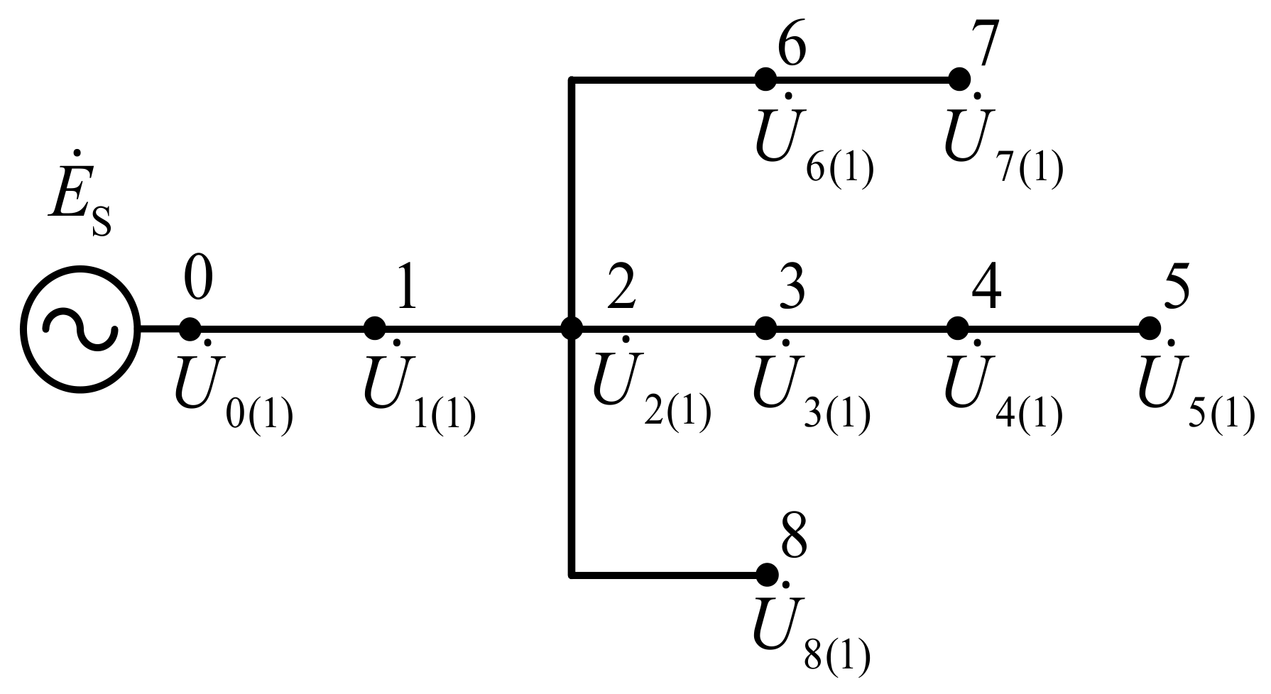
To analyze the variation pattern of the NPSVMD with respect to fault location after a fault occurs, this paper uses the 9-node radial distribution network shown in Figure 1 as an example. Under normal system operating conditions, Node 0 serves as the reference node, while nodes 1 through 8 are the network nodes.

Under normal system operating conditions, the current balance equations for Nodes 1 through 8 can be formulated in accordance with Kirchhoff’s Current Law (KCL).

$$\left\{\begin{array}{l}{\dot{I}}_{1(1)}={\displaystyle \frac{{\dot{U}}_{0(1)}-{\dot{U}}_{1(1)}}{Z_0}}-{\displaystyle \frac{{\dot{U}}_{1(1)}-{\dot{U}}_{2(1)}}{Z_{1\text{-}2}}}\hfill \\ {\dot{I}}_{2(1)}={\displaystyle \frac{{\dot{U}}_{1(1)}-{\dot{U}}_{2(1)}}{Z_{1\text{-}2}}}-{\displaystyle \frac{{\dot{U}}_{2(1)}-{\dot{U}}_{3(1)}}{Z_{2\text{-}3}}}-{\displaystyle \frac{{\dot{U}}_{2(1)}-{\dot{U}}_{8(1)}}{Z_{2\text{-}8}}}-{\displaystyle \frac{{\dot{U}}_{2(1)}-{\dot{U}}_{6(1)}}{Z_{2\text{-}6}}}\hfill \\ {\dot{I}}_{3(1)}={\displaystyle \frac{{\dot{U}}_{2(1)}-{\dot{U}}_{3(1)}}{Z_{2\text{-}3}}}-{\displaystyle \frac{{\dot{U}}_{3(1)}-{\dot{U}}_{4(1)}}{Z_{3\text{-}4}}}\hfill \\ {\dot{I}}_{4(1)}={\displaystyle \frac{{\dot{U}}_{3(1)}-{\dot{U}}_{4(1)}}{Z_{3\text{-}4}}}-{\displaystyle \frac{{\dot{U}}_{4(1)}-{\dot{U}}_{5(1)}}{Z_{4\text{-}5}}}\hfill \\ {\dot{I}}_{5(1)}={\displaystyle \frac{{\dot{U}}_{4(1)}-{\dot{U}}_{5(1)}}{Z_{4\text{-}5}}}\hfill \\ {\dot{I}}_{6(1)}={\displaystyle \frac{{\dot{U}}_{2(1)}-{\dot{U}}_{6(1)}}{Z_{2\text{-}6}}}-{\displaystyle \frac{{\dot{U}}_{6(1)}-{\dot{U}}_{7(1)}}{Z_{6\text{-}7}}}\hfill \\ {\dot{I}}_{7(1)}={\displaystyle \frac{{\dot{U}}_{6(1)}-{\dot{U}}_{7(1)}}{Z_{6\text{-}7}}}\hfill \\ {\dot{I}}_{8(1)}={\displaystyle \frac{{\dot{U}}_{2(1)}-{\dot{U}}_{8(1)}}{Z_{2\text{-}8}}}\hfill \end{array}\right.$$

(1)

where ${\dot{U}}_{i(1)}$ denotes the NPSV at node i, ${\dot{I}}_{i(1)}$ denotes the NPSC injected into node i, Z₀ represents the equivalent positive-sequence impedance (EPSI) between the system source and Node 0, and Z_1-2, Z_2-3, Z_3-4, Z_4-5, Z_2-6, Z_6-7 and Z_2-8 denote the line positive-sequence impedance values(LPSIV) between the corresponding node pairs, respectively.

After rearrangement, the NPSV can be expressed as:

$$\left\{\begin{array}{l}{\dot{U}}_{1(1)}-{\dot{U}}_{0(1)}=-Z_0{\dot{A}}_1\hfill \\ {\dot{U}}_{2(1)}-{\dot{U}}_{0(1)}=-Z_0{\dot{A}}_1-Z_{1\text{-}2}{\dot{A}}_2\hfill \\ {\dot{U}}_{3(1)}-{\dot{U}}_{0(1)}=-Z_0{\dot{A}}_1-Z_{1\text{-}2}{\dot{A}}_2-Z_{2\text{-}3}{\dot{A}}_3\hfill \\ {\dot{U}}_{4(1)}-{\dot{U}}_{0(1)}=-Z_0{\dot{A}}_1-Z_{1\text{-}2}{\dot{A}}_2-Z_{2\text{-}3}{\dot{A}}_3-Z_{3\text{-}4}{\dot{A}}_4\hfill \\ {\dot{U}}_{5(1)}-{\dot{U}}_{0(1)}=-Z_0{\dot{A}}_1-Z_{1\text{-}2}{\dot{A}}_2-Z_{2\text{-}3}{\dot{A}}_3-Z_{3\text{-}4}{\dot{A}}_4-Z_{4\text{-}5}{\dot{A}}_5\hfill \\ {\dot{U}}_{6(1)}-{\dot{U}}_{0(1)}=-Z_0{\dot{A}}_1-Z_{1\text{-}2}{\dot{A}}_2-Z_{2\text{-}6}{\dot{A}}_6\hfill \\ {\dot{U}}_{7(1)}-{\dot{U}}_{0(1)}=-Z_0{\dot{A}}_1-Z_{1\text{-}2}{\dot{A}}_2-Z_{2\text{-}6}{\dot{A}}_6-Z_{6\text{-}7}{\dot{A}}_7\hfill \\ {\dot{U}}_{8(1)}-{\dot{U}}_{0(1)}=-Z_0{\dot{A}}_1-Z_{1\text{-}2}{\dot{A}}_2-Z_{2\text{-}8}{\dot{A}}_8\hfill \end{array}\right.$$

(2)

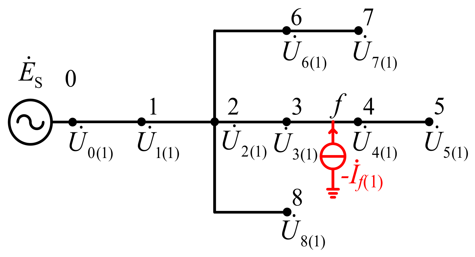
when a fault occurs on a line between nodes in the distribution network, a fault node must be added to the system’s original topology, which causes both the order and the elements of the PSIM to change. If a fault occurs on the line between Node 3 and Node 4, the distribution network model at that time is shown in Figure 2.

After a fault occurs, given the known fault location, the KCL equations for each node in the system are:

$$\left\{\begin{array}{l}{\dot{I}}_{1(1)}^{\prime }={\displaystyle \frac{{\dot{U}}_{0(1)}^{\prime }-{\dot{U}}_{1(1)}^{\prime }}{Z_0}}-{\displaystyle \frac{{\dot{U}}_{1(1)}^{\prime }-{\dot{U}}_{2(1)}^{\prime }}{Z_{1\text{-}2}}}\hfill \\ {\dot{I}}_{2(1)}^{\prime }={\displaystyle \frac{{\dot{U}}_{1(1)}^{\prime }-{\dot{U}}_{2(1)}^{\prime }}{Z_{1\text{-}2}}}-{\displaystyle \frac{{\dot{U}}_{2(1)}^{\prime }-{\dot{U}}_{3(1)}^{\prime }}{Z_{2\text{-}3}}}-{\displaystyle \frac{{\dot{U}}_{2(1)}^{\prime }-U_{8(1)}^{\prime }}{Z_{2\text{-}8}}}-{\displaystyle \frac{{\dot{U}}_{2(1)}^{\prime }-U_{6(1)}^{\prime }}{Z_{2\text{-}6}}}\hfill \\ \begin{array}{l}{\dot{I}}_{3(1)}^{\prime }={\displaystyle \frac{{\dot{U}}_{2(1)}^{\prime }-{\dot{U}}_{3(1)}^{\prime }}{Z_{2\text{-}3}}}-{\displaystyle \frac{{\dot{U}}_{3(1)}^{\prime }-{\dot{U}}_{f(1)}}{Z_{3\text{-}f}}}\\ {\dot{I}}_{f(1)}={\displaystyle \frac{{\dot{U}}_{3(1)}^{\prime }-{\dot{U}}_{f(1)}}{Z_{3\text{-}f}}}-{\displaystyle \frac{{\dot{U}}_{f(1)}-{\dot{U}}_{4(1)}^{\prime }}{Z_{f\text{-}4}}}\end{array}\hfill \\ {\dot{I}}_{4(1)}^{\prime }={\displaystyle \frac{{\dot{U}}_{f(1)}-{\dot{U}}_{4(1)}^{\prime }}{Z_{f\text{-}4}}}-{\displaystyle \frac{{\dot{U}}_{4(1)}^{\prime }-{\dot{U}}_{5(1)}^{\prime }}{Z_{4\text{-}5}}}\hfill \\ {\dot{I}}_{5(1)}^{\prime }={\displaystyle \frac{{\dot{U}}_{4(1)}^{\prime }-{\dot{U}}_{5(1)}^{\prime }}{Z_{4\text{-}5}}}\hfill \\ {\dot{I}}_{6(1)}^{\prime }={\displaystyle \frac{{\dot{U}}_{2(1)}^{\prime }-{\dot{U}}_{6(1)}^{\prime }}{Z_{2\text{-}6}}}-{\displaystyle \frac{{\dot{U}}_{6(1)}^{\prime }-{\dot{U}}_{7(1)}^{\prime }}{Z_{6\text{-}7}}}\hfill \\ {\dot{I}}_{7(1)}^{\prime }={\displaystyle \frac{{\dot{U}}_{6(1)}^{\prime }-{\dot{U}}_{7(1)}^{\prime }}{Z_{6\text{-}7}}}\hfill \\ {\dot{I}}_{8(1)}^{\prime }={\displaystyle \frac{{\dot{U}}_{2(1)}^{\prime }-{\dot{U}}_{8(1)}^{\prime }}{Z_{2\text{-}8}}}\hfill \end{array}\right.$$

(3)

where ${\dot{U}}_{i(1)}^{\prime }$ denotes the NPSV at node i after the fault, ${{\dot{I}}^{\prime }}_{i(1)}$ denotes the measured NPSC at node i after the fault, Z_3-f denotes the LPSIV between Node 3 and the fault point f, Z_f-4 denotes the LPSIV between the fault point f and Node 4, and ${\dot{U}}_{f(1)}$ and ${\dot{I}}_{f(1)}$ denote the NPSV and NPSC at the fault location, respectively.

After rearrangement, the NPSV following the fault can be expressed as:

$$\left\{\begin{array}{l}{\dot{U}}_{1(1)}^{\prime }-{\dot{U}}_{0(1)}^{\prime }=-Z_{0\text{-}1}({\dot{A}}_1^{\prime }+{\dot{I}}_{f(1)})\hfill \\ {\dot{U}}_{2(1)}^{\prime }-{\dot{U}}_{0(1)}^{\prime }=-Z_0({\dot{A}}_1^{\prime }+{\dot{I}}_{f(1)})-Z_{1\text{-}2}({\dot{A}}_2^{\prime }+{\dot{I}}_{f(1)})\hfill \\ {\dot{U}}_{3(1)}^{\prime }-{\dot{U}}_{0(1)}^{\prime }=-Z_0({\dot{A}}_1^{\prime }+{\dot{I}}_{f(1)})-Z_{1\text{-}2}({\dot{A}}_2^{\prime }+{\dot{I}}_{f(1)})-Z_{2\text{-}3}({\dot{A}}_3^{\prime }+{\dot{I}}_{f(1)})\hfill \\ {\dot{U}}_{f(1)}^{\prime }-{\dot{U}}_{0(1)}^{\prime }=-Z_0({\dot{A}}_1^{\prime }+{\dot{I}}_{f(1)})-Z_{1\text{-}2}({\dot{A}}_2^{\prime }+{\dot{I}}_{f(1)})-Z_{2\text{-}3}({\dot{A}}_3^{\prime }+{\dot{I}}_{f(1)})-Z_{3\text{-}f}({\dot{I}}_{f(1)}+{\dot{A}}_4^{\prime })\hfill \\ \begin{array}{ll}{\dot{U}}_{4(1)}^{\prime }-{\dot{U}}_{0(1)}^{\prime }=& -Z_0({\dot{A}}_1^{\prime }+{\dot{I}}_{f(1)})-Z_{1\text{-}2}({\dot{A}}_2^{\prime }+{\dot{I}}_{f(1)})-Z_{2\text{-}3}({\dot{A}}_3^{\prime }+{\dot{I}}_{f(1)})-Z_{3\text{-}f}({\dot{I}}_{f(1)}+{\dot{A}}_4^{\prime })\\ & -Z_{f\text{-}4}{\dot{A}}_4^{\prime }\end{array}\hfill \\ \begin{array}{ll}{\dot{U}}_{5(1)}^{\prime }-{\dot{U}}_{0(1)}^{\prime }=& -Z_0({\dot{A}}_1^{\prime }+{\dot{I}}_{f(1)})-Z_{1\text{-}2}({\dot{A}}_2^{\prime }+{\dot{I}}_{f(1)})-Z_{2\text{-}3}({\dot{A}}_3^{\prime }+{\dot{I}}_{f(1)})-Z_{3\text{-}f}({\dot{I}}_{f(1)}+{\dot{A}}_4^{\prime })\\ & -Z_{f\text{-}4}{\dot{A}}_4^{\prime }-Z_{45}{\dot{A}}_5^{\prime }\end{array}\hfill \\ {\dot{U}}_{6(1)}^{\prime }-{\dot{U}}_{0(1)}^{\prime }=-Z_0({\dot{A}}_1^{\prime }+{\dot{I}}_{f(1)})-Z_{1\text{-}2}({\dot{A}}_2^{\prime }+{\dot{I}}_{f(1)})-Z_{2\text{-}6}{\dot{A}}_6^{\prime }\hfill \\ {\dot{U}}_{7(1)}^{\prime }-{\dot{U}}_{0(1)}^{\prime }=-Z_0({\dot{A}}_1^{\prime }+{\dot{I}}_{f(1)})-Z_{1\text{-}2}({\dot{A}}_2^{\prime }+{\dot{I}}_{f(1)})-Z_{2\text{-}6}{\dot{A}}_6^{\prime }-Z_{6\text{-}7}{\dot{A}}_7^{\prime }\hfill \\ {\dot{U}}_{8(1)}^{\prime }-{\dot{U}}_{0(1)}^{\prime }=-Z_0({\dot{A}}_1^{\prime }+{\dot{I}}_{f(1)})-Z_{1\text{-}2}({\dot{A}}_2^{\prime }+{\dot{I}}_{f(1)})-Z_{2\text{-}8}{\dot{A}}_8^{\prime }\hfill \end{array}\right.$$

(4)

$$\left\{\begin{array}{l}{\dot{I}}_{1(1)}^{\prime }={\displaystyle \frac{{\dot{U}}_{0(1)}^{″}-{\dot{U}}_{1(1)}^{″}}{Z_0}}-{\displaystyle \frac{{\dot{U}}_{1(1)}^{″}-{\dot{U}}_{2(1)}^{″}}{Z_{1\text{-}2}}}\hfill \\ {\dot{I}}_{2(1)}^{\prime }={\displaystyle \frac{{\dot{U}}_{1(1)}^{″}-{\dot{U}}_{2(1)}^{″}}{Z_{1\text{-}2}}}-{\displaystyle \frac{{\dot{U}}_{2(1)}^{″}-{\dot{U}}_{3(1)}^{″}}{Z_{2\text{-}3}}}-{\displaystyle \frac{{\dot{U}}_{2(1)}^{″}-U_{8(1)}^{\prime }}{Z_{2\text{-}8}}}-{\displaystyle \frac{{\dot{U}}_{2(1)}^{″}-U_{6(1)}^{\prime }}{Z_{2\text{-}6}}}\hfill \\ {\dot{I}}_{3(1)}^{\prime }={\displaystyle \frac{{\dot{U}}_{2(1)}^{″}-{\dot{U}}_{3(1)}^{″}}{Z_{2\text{-}3}}}-{\displaystyle \frac{{\dot{U}}_{3(1)}^{″}-{\dot{U}}_{4(1)}^{″}}{Z_{3\text{-}4}}}\hfill \\ {\dot{I}}_{4(1)}^{\prime }={\displaystyle \frac{{\dot{U}}_{3(1)}^{″}-{\dot{U}}_{4(1)}^{″}}{Z_{f\text{-}4}}}-{\displaystyle \frac{{\dot{U}}_{4(1)}^{″}-{\dot{U}}_{5(1)}^{″}}{Z_{4\text{-}5}}}\hfill \\ {\dot{I}}_{5(1)}^{\prime }={\displaystyle \frac{{\dot{U}}_{4(1)}^{″}-{\dot{U}}_{5(1)}^{″}}{Z_{4\text{-}5}}}\hfill \\ {\dot{I}}_{6(1)}^{\prime }={\displaystyle \frac{{\dot{U}}_{2(1)}^{″}-{\dot{U}}_{6(1)}^{″}}{Z_{2\text{-}6}}}-{\displaystyle \frac{{\dot{U}}_{6(1)}^{″}-{\dot{U}}_{7(1)}^{″}}{Z_{6\text{-}7}}}\hfill \\ {\dot{I}}_{7(1)}^{\prime }={\displaystyle \frac{{\dot{U}}_{6(1)}^{″}-{\dot{U}}_{7(1)}^{″}}{Z_{6\text{-}7}}}\hfill \\ {\dot{I}}_{8(1)}^{\prime }={\displaystyle \frac{{\dot{U}}_{2(1)}^{″}-{\dot{U}}_{8(1)}^{″}}{Z_{2\text{-}8}}}\hfill \end{array}\right.$$

(5)

As shown in Equation (4), given the known fault location, the current balance equations for each node can be formulated to determine the NPSV. However, since the relative relationship between the fault location and the nodes is unknown prior to fault location, it is impossible to establish a new impedance relationship among the nodes after the fault, nor is it possible to directly obtain the voltage and current measurement data at the fault location. Therefore, only the measured NPSC values after the fault can be utilized, in conjunction with the pre-fault PSIM of the system under normal operating conditions, to derive the IMNPSV. After the fault occurs, the original nodes of the system still satisfy KCL, and the corresponding KCL equations can be expressed as Equation (5).

As shown in Equation (5), ${\dot{U}}_{i(1)}^{″}$ is defined as the IMNPSV after the fault (i = 1~8). Node 0 is the reference node; therefore, ${\dot{U}}_{0(1)}^{″}$ is a known quantity and ${\dot{U}}_{0(1)}^{″}={\dot{U}}_{0(1)}^{\prime }$.

Rearranging yields Equation (6):

$$\left\{\begin{array}{l}{\dot{U}}_{1(1)}^{″}-{\dot{U}}_{0(1)}^{″}=-Z_0{\dot{A}}_1^{\prime }\hfill \\ {\dot{U}}_{2(1)}^{″}-{\dot{U}}_{0(1)}^{″}=-Z_0{\dot{A}}_1^{\prime }\text{-}{Z}_{12}{\dot{A}}_2^{\prime }\hfill \\ {\dot{U}}_{3(1)}^{″}-{\dot{U}}_{0(1)}^{″}=-Z_0{\dot{A}}_1^{\prime }-Z_{12}{\dot{A}}_2^{\prime }-Z_{23}{\dot{A}}_3^{\prime }\hfill \\ {\dot{U}}_{4(1)}^{″}-{\dot{U}}_{0(1)}^{″}=-Z_0{\dot{A}}_1^{\prime }-Z_{12}{\dot{A}}_2^{\prime }-Z_{23}{\dot{A}}_3^{\prime }-Z_{34}{\dot{A}}_4^{\prime }\hfill \\ \begin{array}{l}{\dot{U}}_{5(1)}^{″}-{\dot{U}}_{0(1)}^{″}=-Z_0{\dot{A}}_1^{\prime }-Z_{12}{\dot{A}}_2^{\prime }-Z_{23}{\dot{A}}_3^{\prime }-Z_{34}{\dot{A}}_4^{\prime }-Z_{45}{\dot{A}}_5^{\prime }\\ {\dot{U}}_{6(1)}^{″}-{\dot{U}}_{0(1)}^{″}=-Z_0{\dot{A}}_1^{\prime }-Z_{12}{\dot{A}}_2^{\prime }-Z_{26}{\dot{A}}_6^{\prime }\end{array}\hfill \\ {\dot{U}}_{7(1)}^{″}-{\dot{U}}_{0(1)}^{″}=-Z_0{\dot{A}}_1^{\prime }-Z_{12}{\dot{A}}_2^{\prime }-Z_{26}{\dot{A}}_6^{\prime }-Z_{67}{\dot{A}}_7^{\prime }\hfill \\ {\dot{U}}_{8(1)}^{″}-{\dot{U}}_{0(1)}^{″}=-Z_0{\dot{A}}_1^{\prime }-Z_{12}{\dot{A}}_2^{\prime }-Z_{28}{\dot{A}}_8^{\prime }\hfill \end{array}\right.$$

(6)

Subtracting Equation (4) from Equation (6), comparing the IMNPSV after the fault with their corresponding direct measurements, yields a difference that is NPSVMD. The result is given by:

$$\left\{\begin{array}{l}\left[{\dot{U}}_{1(1)}^{″}-{\dot{U}}_{0(1)}^{″}\right]-\left[{\dot{U}}_{1(1)}^{\prime }-{\dot{U}}_{0(1)}^{\prime }\right]=Z_0{\dot{I}}_{f(1)}\hfill \\ \left[{\dot{U}}_{2(1)}^{″}-{\dot{U}}_{0(1)}^{″}\right]-\left[{\dot{U}}_{2(1)}^{\prime }-{\dot{U}}_{0(1)}^{\prime }\right]=(Z_0+Z_{1\text{-}2}){\dot{I}}_{f(1)}\hfill \\ \left[{\dot{U}}_{3(1)}^{″}-{\dot{U}}_{0(1)}^{″}\right]-\left[{\dot{U}}_{3(1)}^{\prime }-{\dot{U}}_{0(1)}^{\prime }\right]=(Z_0+Z_{1\text{-}2}+Z_{2\text{-}3}){\dot{I}}_{f(1)}\hfill \\ \left[{\dot{U}}_{4(1)}^{″}-{\dot{U}}_{0(1)}^{″}\right]-\left[{\dot{U}}_{4(1)}^{\prime }-{\dot{U}}_{0(1)}^{\prime }\right]=(Z_0+Z_{1\text{-}2}+Z_{2\text{-}3}+Z_{3\text{-}f}){\dot{I}}_{f(1)}\hfill \\ \left[{\dot{U}}_{5(1)}^{″}-{\dot{U}}_{0(1)}^{″}\right]-\left[{\dot{U}}_{5(1)}^{\prime }-{\dot{U}}_{0(1)}^{\prime }\right]=(Z_0+Z_{1\text{-}2}+Z_{2\text{-}3}+Z_{3\text{-}f}){\dot{I}}_{f(1)}\hfill \\ \left[{\dot{U}}_{6(1)}^{″}-{\dot{U}}_{0(1)}^{″}\right]-\left[{\dot{U}}_{6(1)}^{\prime }-{\dot{U}}_{0(1)}^{\prime }\right]=(Z_0+Z_{1\text{-}2}){\dot{I}}_{f(1)}\hfill \\ \left[{\dot{U}}_{7(1)}^{″}-{\dot{U}}_{0(1)}^{″}\right]-\left[{\dot{U}}_{7(1)}^{\prime }-{\dot{U}}_{0(1)}^{\prime }\right]=(Z_0+Z_{1\text{-}2}){\dot{I}}_{f(1)}\hfill \\ \left[{\dot{U}}_{8(1)}^{″}-{\dot{U}}_{0(1)}^{″}\right]-\left[{\dot{U}}_{8(1)}^{\prime }-{\dot{U}}_{0(1)}^{\prime }\right]=(Z_0+Z_{1\text{-}2}){\dot{I}}_{f(1)}\hfill \end{array}\right.$$

(7)

In this context, the indirect measurement is obtained by computing the DMNPSV together with the impedance matrix of the system under normal operating conditions, whereas the direct measurement refers to the data acquired directly from the measurement device. As shown in Equation (7), when a fault occurs on the line between Node 3 and Node 4, the NPSVMD at Node 4 and Node 5 are equal, and both are greater than those at Nodes 1, 2, 3, 6, 7, and 8.

For a radial distribution network with a single source node s, if a single short-circuit fault occurs at point f, the NPSVMDs of all nodes located downstream of f are identical and attain the maximum value among all nodes, provided that the network is represented by a positive-sequence radial equivalent model and the line positive-sequence impedances have non-negative resistance and reactance.

For any node i, there exists a unique path P(s,i) from the source node to node i. Let P(s,f) denote the unique path from the source node to the fault point f. In a radial network, the positive-sequence mutual impedance between node i and the fault point f is equal to the accumulated impedance along the common part of P(s,i) and P(s,f), namely:

$$Z_{if}^c={\displaystyle \sum _{e\in P(s,i)\cap P(s,f)}{z}_e},$$

(8)

where z_e is the positive-sequence impedance of line section e.

Under the equivalent positive-sequence fault-current injection model, the NPSVMD at node iii can be expressed as:

$$D_i=\left|I_f{Z}_{if}^c\right|$$

(9)

where I_f is the equivalent positive-sequence fault current. Therefore, the relative magnitude of D_i is determined by the common-path impedance $Z_{if}^c$.

If node i is located downstream of the fault point fff, the source-to-fault path P(s,f) is completely contained in the source-to-node path P(s,i).

$$P(s,i)\cap P(s,f)=P(s,f)$$

(10)

Therefore, the common-path impedance of downstream node i is:

$$Z_{i\mathrm{f}}^c=Z_{sf}$$

(11)

Thus, for any downstream node i of the fault point, we have:

$$D_i=\mid I_f{Z}_{sf}\mid ,$$

(12)

where Z_sf is the accumulated positive-sequence impedance from the source node to the fault point. This result is independent of the specific downstream node i. Thus, all downstream nodes have identical NPSVMD values.

For a node k located upstream of the fault point or on another lateral branch, the common path between P(s,k) and P(s,f) is only a proper subset of P(s,f). Let b be the end node of their common path, then we have:

$$Z_{kf}^c=Z_{sb},Z_{sf}=Z_{sb}+Z_{bf}$$

(13)

where Z_bf is the accumulated impedance from b to the fault point. Since the resistance and reactance of the line positive-sequence impedance are non-negative, and there are no zero-impedance branches in the path, the cumulative path impedance increases monotonically along the feeder direction, that is:

$$\mid Z_{kf}^c\mid <\mid Z_{sf}\mid$$

(14)

Thus, we obtain:

$$D_k<\mid I_f{Z}_{sf}\mid$$

(15)

Therefore, the NPSVMDs of downstream nodes are equal and larger than those of upstream or lateral-branch nodes. This proves the equal-and-maximum NPSVMD property for a general radial distribution network under the stated assumptions.

Under the stated radial-network assumptions, the NPSVMD values of nodes downstream of the fault point are theoretically equal and attain the maximum value, because these nodes share the same source-to-fault common path impedance. For upstream nodes or nodes located on other lateral branches, the common-path impedance is only a proper subset of the source-to-fault path impedance, resulting in smaller NPSVMD values.

3. Data Self-Synchronization Issues Between Different Measurement Terminals

Although the above analysis lays a theoretical foundation, in practical μPMU data acquisition, even small synchronization errors can be amplified and destroy the relative magnitudes of the features. Therefore, a rigorous data self-synchronization calibration mechanism must be established before faulted line selection and distance estimation.

3.1. Analysis of Measurement Errors in the μPMU

Sinusoidal quantities are typically represented as complex-valued phasors, with the modulus denoting the signal amplitude and the argument representing its initial phase. Synchronous phasors, obtained by synchronously sampling voltage and current signals at different nodes under a unified time reference, ensure temporal phase consistency across measuring points. Since there are definite phase relationships between the voltages and currents at different nodes in a power distribution network, obtaining synchronous phasors using a unified time reference can more accurately reflect the system’s operating state.

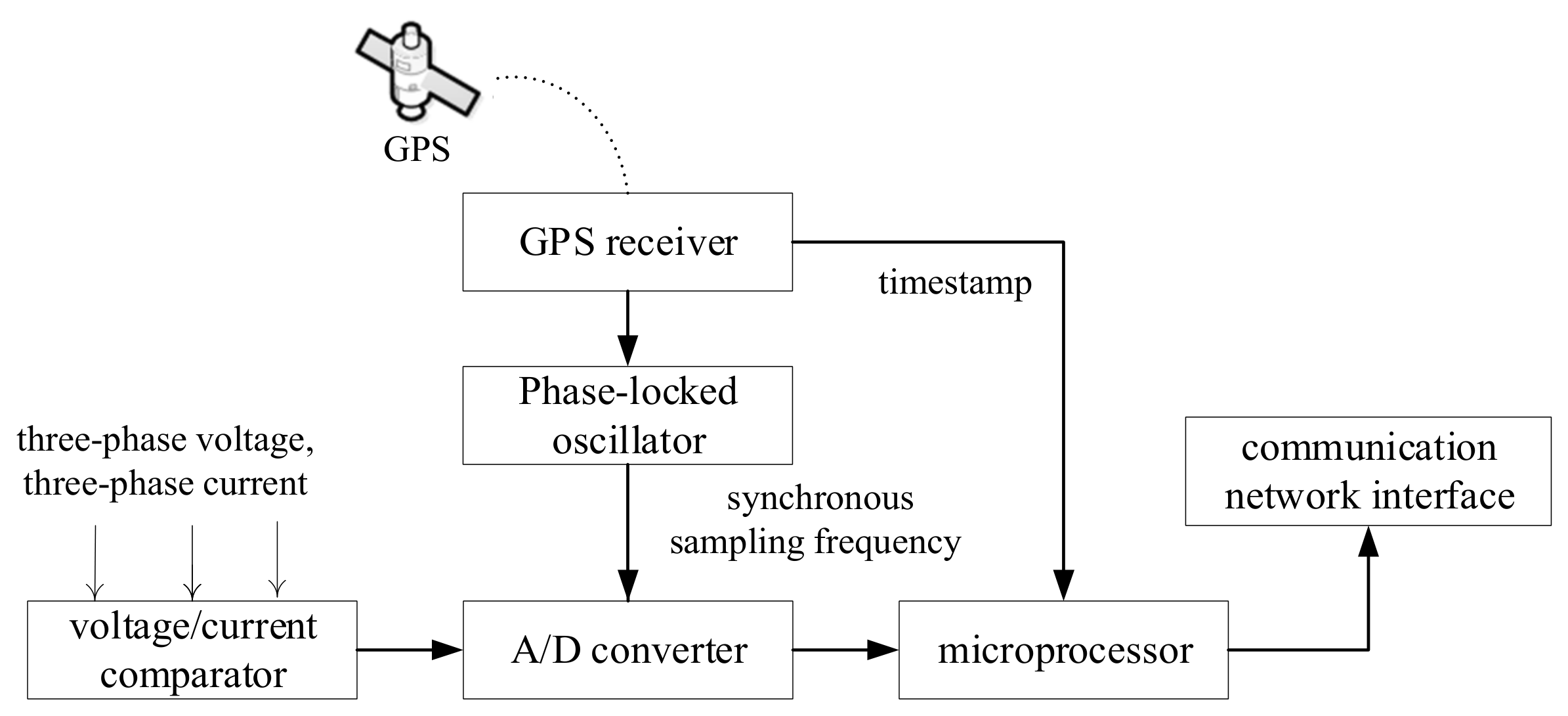
The μPMU is a dedicated device for synchronous phasor measurement and output, with additional dynamic process recording functionality. As illustrated in Figure 3, its hardware architecture comprises four main units: signal conversion, data sampling, data processing, and communication. In operation, voltage and current signals from the distribution network are scaled via voltage and current transformers before being fed to the A/D converter, which performs synchronous sampling triggered by GPS synchronization pulses. The resulting digital signals are then processed in a microprocessor-based unit for phasor calculation and feature extraction. Finally, the processed data is either transmitted to the central control center over the communication network or stored and displayed locally.

Although μPMUs offer high measurement accuracy, measurement errors are inevitable in practical applications. The measurement accuracy of μPMUs is influenced by a variety of factors, including hardware components, data sampling, timing systems, and phasor estimation algorithms. Since the fault location methods discussed later in this paper rely on the phasor relationships between voltage and current at multiple measurement nodes, it is necessary to analyze the various sources of error.

The measurement errors of μPMU can be classified into four categories: sensor error, data sampling and analog-to-digital conversion error, synchronization system error, and phasor estimation algorithm error. Different types of errors affect measurement results in different ways; some errors primarily affect amplitude measurements, while others mainly manifest as phase angle deviations.

Sensor error is a major source of measurement errors in μPMU. The voltage and current signals in distribution networks need to be converted through voltage transformers, current transformers and signal conditioning circuits. The transformer ratio error, phase delay error, and parameter deviation of devices in the conditioning circuit will cause deviations in the amplitude and phase angle of input signals from their true values. Since sensor errors directly act on the original measured signals, they are generally one of the main factors affecting the measurement accuracy of μPMU.

Data sampling and analog-to-digital conversion can introduce inherent errors. Insufficient sampling frequency, sampling time jitter and limited quantization bits all degrade the measurement accuracy. Nevertheless, most A/D converters adopt 14-bit or 16-bit devices; their quantization error is far smaller than sensor error and algorithmic error, and is not a dominant factor in the context of this study.

Synchronization system errors are mainly manifested as a phase angle offset caused by time deviation. The core of synchronous phasor measurement lies in a unified time reference. Time timing deviation, communication delay and other factors will lead to asynchronous outputs among multiple μPMUs, thereby resulting in phase angle deviations. Under normal timing conditions, the synchronization error of a single device is small. However, fault location in distribution networks relies on phasor relationships of multiple measuring points; even minor synchronization errors can be amplified, affecting location accuracy, and thus require special attention.

Phasor estimation algorithm error is also a critical influencing factor. Common phasor calculation methods include the zero-crossing detection method, least squares method, discrete Fourier transform method, and so on. Among them, the discrete Fourier transform method is widely applied due to its strong robustness and convenient engineering implementation. Algorithm errors are closely related to the operating state of the power grid. In the presence of frequency offset, harmonic interference and other disturbances, the accuracy of amplitude and phase angle will deteriorate, which constitutes an important component of μPMU systematic errors.

In summary, the main sources of μPMU measurement errors include sensor errors, synchronization system errors, and phasor estimation algorithm errors. Among them, sensor errors directly affect the measurement accuracy of both amplitude and phase angle; algorithm errors are closely related to signal quality and operating conditions; while synchronization system errors are mainly reflected in the phase inconsistency among different measuring points.

For the fault location method proposed in this paper, the relative relationship of phasors among multiple measuring points is more critical than the measurement accuracy of a single point. Therefore, the synchronization deviation between different measurement terminals deserves special attention. To facilitate the subsequent analysis, the error ranges of current and voltage measurements are specified in

Table 1. Current measurement error.

Measured Current	$0.01{\mathit{I}}_{\mathit{n}}<\mathit{I}<0.2{\mathit{I}}_{\mathit{n}}$	$0.2{\mathit{I}}_{\mathit{n}}<\mathit{I}<0.5{\mathit{I}}_{\mathit{n}}$	$0.5{\mathit{I}}_{\mathit{n}}<\mathit{I}<1.2{\mathit{I}}_{\mathit{n}}$
Maximum error of current amplitude	1.0%	0.5%	0.2%
Maximum error of current phase angle	1°	0.05°	0.5°

and

Table 2. Voltage measurement error.

Measured Current	$0.01{\mathit{U}}_{\mathit{n}}<\mathit{U}<0.2{\mathit{U}}_{\mathit{n}}$	$0.2{\mathit{U}}_{\mathit{n}}<\mathit{U}<0.5{\mathit{U}}_{\mathit{n}}$	$0.5{\mathit{U}}_{\mathit{n}}<\mathit{U}<1.2{\mathit{U}}_{\mathit{n}}$
Maximum error of current amplitude	1.0%	0.5%	0.2%
Maximum error of current phase angle	0.5°	0.5°	0.5°

, respectively.

3.2. Data Synchronization Issues Between Different Measurement Terminals

The fault location method proposed in this paper relies on synchronous measurement data of voltage and current phasors at multiple measuring points, thus imposing high requirements on the time consistency of data from different measuring points. However, in practical applications, affected by factors such as time synchronization deviation, communication delay, or internal device processing errors, there may be certain synchronization deviations between data from different measuring points, which further manifest as phase angle errors.

Given that the synchronization accuracy of existing measurement devices typically keeps errors within 1°, this paper takes into account the synchronization error between data from both ends during method analysis and application. It proposes a self-synchronization method that uses station-end data as the reference to correct synchronization errors between different measurement terminals.

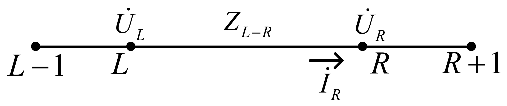
To illustrate the basic principle of the proposed method, the two-port network shown in Figure 4 is taken as an example for analysis. The left and right end nodes of the section are denoted as L and R, respectively. The voltages at the left and right ends are ${\dot{U}}_L$ and ${\dot{U}}_R$, and the measured current at the right end is ${\dot{I}}_R$. The line impedance between nodes L and R is Z_L-R, and the synchronization error angle between the voltage and current phasors at the start and end of the section is $\theta$. According to the voltage drop relationship of the two-port network, an equality relationship between the measurements at both ends of the section can be established.

If the data at both ends are perfectly synchronized, the section relational expression constructed from the line parameters and measured phasors should strictly satisfy the physical constraints of the circuit; when there is a synchronization deviation between the two ends, this constraint relationship will be violated.

Based on this, using the phase angle information of the left-hand-side vector as a reference, the right-hand-side measured vector is uniformly multiplied by the synchronization error correction factor, thereby explicitly introducing the unknown synchronization error angle into the section equation. Since, in theory, both ends of the section should satisfy the same circuit relationship, an equation for solving the synchronization error angle can be established from the corrected equation.

$${\dot{U}}_L-{\dot{U}}_R{e}^{j\theta }=Z_{L-R}{\dot{I}}_R{e}^{j\theta }$$

(16)

Therefore, we can obtain:

$${\displaystyle \frac{{\dot{U}}_L-{\dot{U}}_R{e}^{j\theta }}{Z_{L-R}{\dot{I}}_R{e}^{j\theta }}}=1$$

(17)

Furthermore, since the imaginary part of the expression on the left-hand side of the equation must be zero, the phase error angle between the phasors at the beginning and end of the section can be calculated, thereby enabling phase correction of the measurement data downstream of the section.

$$\mathrm{Im}\left({\displaystyle \frac{{\dot{U}}_L-{\dot{U}}_R{e}^{j\theta }}{Z_{L-R}{\dot{I}}_R{e}^{j\theta }}}\right)=0$$

(18)

Given that distribution networks typically have a radial or weakly looped structure, this paper employs a method of self-synchronization across the entire network by using a reference node as the baseline and performing recursive correction node by node in the downstream direction. Specifically, a measurement point on the substation side or the main power supply side can be selected as the reference node, assuming that the time reference of its measurement data is reliable. Then, based on the network topology, the synchronization error between adjacent measurement nodes is calculated along the line direction, and the phasor data of downstream nodes is calibrated sequentially. Through this process, measurement data from multiple points across the entire network can be unified under a single time reference, thereby reducing the impact of synchronization errors between measurement devices on fault location.

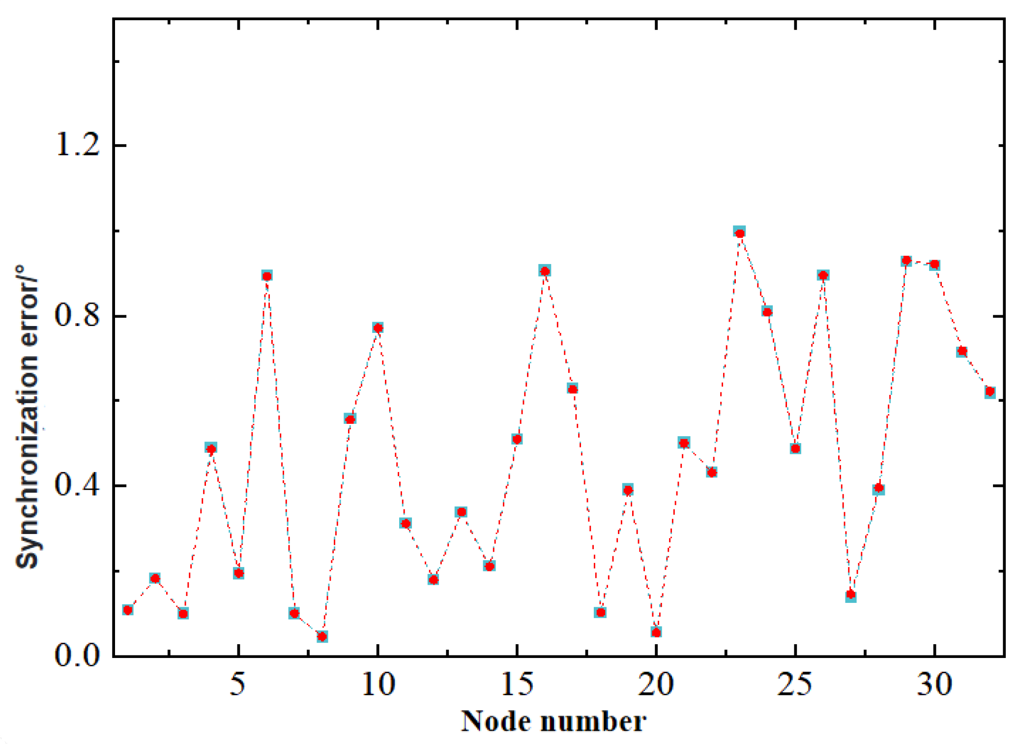
To verify the effectiveness of the proposed self-synchronization method, this paper conducts a simulation analysis using the IEEE 33-node distribution network as an example. Synchronization errors within the range of 0–1° were introduced into the electrical quantities of nodes 1 through 32, and self-synchronization calibration was performed using node 0 as the reference node. Figure 5 shows a comparison of the input values and calculated values when synchronization errors were introduced into all nodes. The green line represents the set value, while the red line represents the calculated value.

As shown in Figure 5, the synchronization error angles of each node calculated by the proposed method are generally consistent with the set values, indicating that the method can accurately estimate the synchronization deviations between different measuring points and correct them.

Table 3. Synchronization error angle after correction.

	Average Synchronization Error/°	Corrected Error/°
Set value	0.46563	0.00015
Calculated value	0.46548

presents the synchronization error angle data after correction. It can be seen that the average synchronization error of the system is reduced from 0.46563° to 0.00015° after calibration, indicating that the proposed method can effectively suppress the synchronization errors between different measurement terminals and provide a more consistent and reliable measurement data foundation for subsequent fault location.

4. Principles for Faulted Line Determination Under Limited Measurement Information

By constructing the relationship between the NPSVMD and the fault location using voltage and current information acquired at each node, fault section location and distance estimation can be achieved.

In practical engineering applications, however, the deployment of measurement devices is typically insufficient to cover all nodes and is generally restricted to critical nodes. Even when the number of measurement nodes is reduced, the magnitude pattern of the NPSVMD among the measurement nodes remains valid; consequently, faulted line identification can still be performed. Nevertheless, a measurement point may not exist upstream of the faulted line. Therefore, an equivalent calculation method for the fault current is introduced, and a distance estimation function is formulated by combining the NPSVMD values from measurement nodes upstream and downstream of the fault location, thereby enabling accurate fault location.

4.1. Principle of Line Identification

In actual distribution networks, it is impractical to install μPMUs at all nodes due to constraints imposed by device cost, communication bandwidth, and maintenance workload. Consequently, in engineering applications, measurement devices are typically deployed only at a subset of critical nodes, rendering the full sequence of deviation magnitudes {D_i} across all nodes unavailable. With the reduced number of measurement nodes, the NPSVMD relationships are no longer established for every node in the system; instead, an NPSVMD analysis model is formulated exclusively for those nodes equipped with μPMUs. Let the set of nodes in the system equipped with μPMUs be denoted as:

$$\mathcal{M}=\left\{m_1,m_2,\cdots ,m_s\right\}$$

(19)

where v denotes the total number of measurement nodes equipped with μPMUs, and v ≤ N.

Under the condition of a reduced number of measurement devices, nodes without installed measurement devices are no longer treated as independently observable nodes. Instead, the nodes equipped with measurement devices form a new v × v impedance matrix Z_m among themselves. The elements of the impedance matrix Z_m no longer represent the local impedance relationship between adjacent physical nodes, but rather denote the equivalent cumulative impedance relationship between the corresponding measurement nodes.

Under the condition of a reduced number of measurement nodes, for any measurement point $m_r\in \mathcal{M}$, its NPSVMD can still be defined as:

$$D_{m_r}=\left|{\dot{U}}_{m_r(1)}^{″}-{\dot{U}}_{m_r(1)}^{\prime }\right|=\left|{\left[Z_{m(1)}{\dot{I}}_{m(1)}^{\prime }\right]}_{m_r}-{\dot{U}}_{m_r(1)}^{\prime }\right|$$

(20)

where ${\dot{U}}_{m_r(1)}^{″}$ and ${\dot{U}}_{m_r(1)}^{\prime }$ denote the IMNPSV and the DMNPSV at measurement point m_r, respectively. $Z_{m(1)}$ represents the PSIM between measurement nodes, and ${\dot{I}}_{m(1)}^{\prime }$ denotes the NPSC.

When a fault occurs, the fault location f lies between two measurement nodes; that is, there exist upstream and downstream measurement nodes relative to the fault position. Therefore, Equation (20) can be simplified to Equation (21).

$$D_{m_r}=\left|{\dot{U}}_{m_r(1)}^{″}-{\dot{U}}_{m_r(1)}^{\prime }\right|=\left|{\displaystyle \sum _{j=1}^N(Z_{m_r{m}_j(1)}-Z_{m_r{m}_j(1)}^{\prime }){\dot{I}}_{m_j(1)}^{\prime }}-Z_{m_{r}f(1)}^{\prime }{\dot{I}}_{f(1)},m_r\in \mathcal{M}\right|$$

(21)

where $Z_{m_r{m}_j(1)}$ denotes the mutual impedance between measurement nodes m_r and m_j within the PSIM Z_m(1) under normal system operating conditions; $Z_{m_r{m}_j(1)}^{\prime }$ denotes the mutual impedance between measurement point m_r and measurement point m_j within the PSIM $Z_{m(1)}^{\prime }$ that relates measurement nodes to the fault location after the fault occurs; and ${\dot{I}}_{m_j(1)}^{\prime }$ denotes the NPSC at measurement point m_j after the fault.

When the measurement point m_r is located upstream of the fault location f, the path from the reference node m_s to the measurement point m_r does not traverse the fault location. Therefore, the mutual impedance between the measurement point m_r and the fault location depends solely on the EPSI $Z_{m_s{m}_r(1)}$ between the measurement point m_r and the reference node m_s. Consequently, its NPSVMD can be expressed as:

$$D_{m_r}=\left|-Z_{m_s{m}_r(1)}{\dot{I}}_{f(1)}\right|,m_r\in {\mathcal{M}}_u$$

(22)

where ${\mathcal{M}}_u$ denotes the set of measurement nodes located upstream of the fault, and $Z_{si(1)}$ represents the EPSI from the reference node m_s to the measurement point m_r.

When the measurement point m_r is located downstream of the fault location f, the path from the reference node m_s to the measurement point m_r inevitably passes through the fault location. Therefore, the mutual impedance between the measurement point m_r and the fault location f depends solely on the EPSI $Z_{m_{s}f(1)}$ between the fault location f and the reference node m_s. By the same reasoning, the mutual impedance between any measurement point downstream of the fault and the fault location f is also determined by $Z_{m_{s}f(1)}$. Consequently, the NPSVMD corresponding to these measurement nodes is equal and can be expressed as:

$$D_{m_r}=\left|-Z_{m_{s}f(1)}{\dot{I}}_{f(1)}\right|,m_r\in {\mathcal{M}}_d$$

(23)

where ${\mathcal{M}}_d$ denotes the set of nodes downstream of the fault point, and $Z_{sf(1)}$ represents the EPSI from reference node m_s to the fault point f.

Therefore, under the condition of a reduced number of measurement nodes, the relationship between the NPSVMD at each measurement point and the fault location remains valid.

The NPSVMD at the measurement nodes m_r satisfies:

$$D_{m_r}=\left|\delta U_{m_r}\right|=\left\{\begin{array}{c}\left|Z_{m_s{m}_r(1)}{\dot{I}}_{f(1)}\right|,m_r\in {\mathcal{M}}_u\\ \left|Z_{m_{o}f(1)}{\dot{I}}_{f(1)}\right|,m_r\in {\mathcal{M}}_d\end{array}\right.$$

(24)

It can be observed from Equation (24) that for measurement nodes located downstream of the fault location, their NPSVMD should reach the global maximum or a value close to the global maximum, whereas for measurement nodes located upstream of the fault location, their deviations are relatively smaller. Based on this pattern, this paper utilizes the distribution characteristics of the NPSVMD at the measurement nodes under the condition of limited measurement information to identify the candidate branch where the fault is located, thereby performing faulted line identification. The algorithm involves only simple numerical calculations and path search, resulting in low computational complexity, which can meet the real-time computing requirements of large-scale distribution networks.

4.2. Principle of Measurement Device Placement

To distinguish the NPSVMD between measurement nodes upstream and downstream of the fault location, the deployment of measurement devices should adhere to the following principles:

(1)

Mandatory installation nodes: ① The outgoing node of the reference source in the distribution network, to ensure the accuracy of the system voltage reference; ② Nodes with three or more branches, to enhance the observability of fault location; ③ Terminal nodes of the network, to guarantee the integrity of the line coverage.

(2)

Optional installation nodes: For nodes on relatively short branch lines, or at the connection points between cable lines and overhead lines, measurement devices may be deployed as appropriate. This helps to mitigate the impact of line parameter variations on fault location accuracy and enhances the capability for local fault detection.

The proposed measurement point placement rule aims to achieve an optimal trade-off between the deployment cost of measuring devices and the fault location accuracy. Although the traditional optimal measurement point configuration strategy can realize the full-network observability, it usually requires a measurement point penetration rate higher than 30% and relies on complex optimization solution processes. Conversely, while concentrating μPMUs solely at feeder terminals can further reduce equipment investment, it significantly weakens the observability of the internal topology of the distribution network, resulting in a marked decline in fault location resolution.

In contrast, the proposed placement strategy preferentially covers the junction nodes of main and branch feeders as well as critical load nodes. In the IEEE 33-bus system, only 8 μPMUs are required. Without solving complex optimization matrices, the proposed strategy can realize accurate fault line identification and high-precision fault location, which remarkably reduces equipment investment and operation maintenance costs. More importantly, relying on the common path search mechanism of NPSVMD, even if the number of measurement nodes is further reduced due to budget constraints in cost-sensitive distribution networks, the proposed algorithm can effectively avoid multiple solutions, misjudgments and location failure. It only degrades the localization resolution steadily from the precise line level to the unique main section level. The proposed placement scheme integrates superior topological distinguishability, low investment cost and high operational reliability, exhibiting comprehensive application advantages.

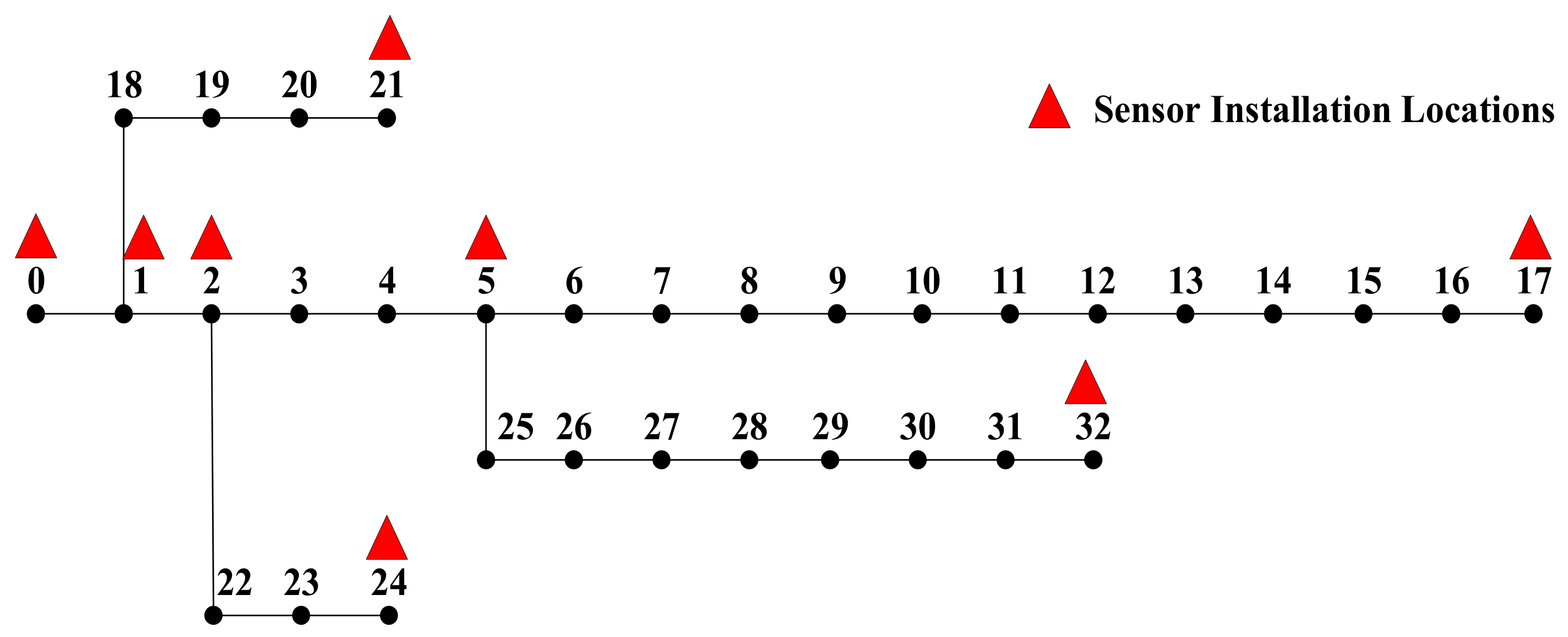
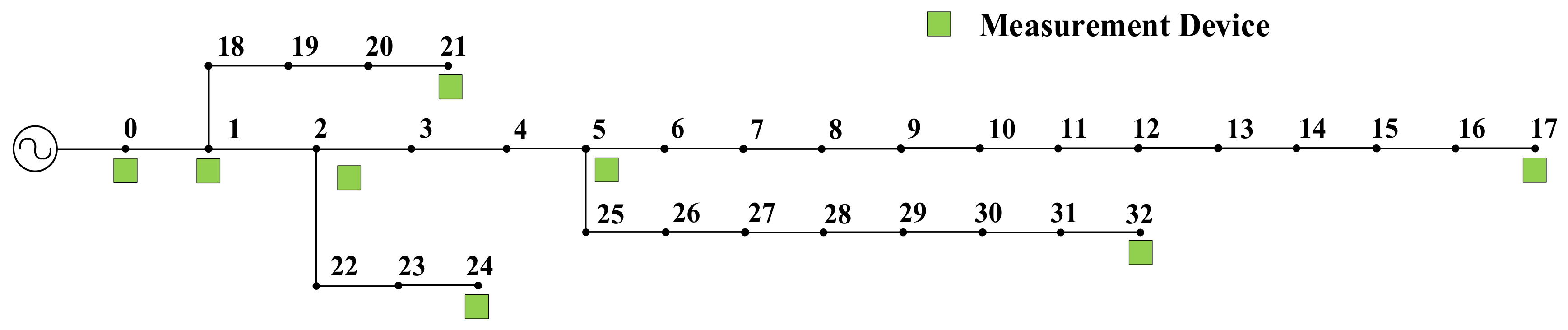
Taking the IEEE 33-node topology shown in Figure 6 as an example and considering a single fault scenario, the mandatory installation nodes that satisfy the principles for measurement device deployment are as follows: ① The outgoing node of the reference source in the distribution network: Node 0; ② Nodes with three or more branches: Nodes 1, 2, and 5; ③ Terminal nodes of the network: Nodes 17, 21, 24, and 32.

To characterize the distribution of the NPSVMD across all measurement nodes, the maximum value among the measurement point deviations is defined as:

$$D_{\max }=\underset{m_r\in \mathcal{M}}{\max }{D}_{m_r}$$

(25)

Considering the influence of measurement errors, parameter inaccuracies, and load fluctuations, a relative margin coefficient $\delta$ is introduced, and the set of measurement nodes with the maximum NPSVMD is defined as:

$${\mathcal{M}}_{\max }=\left\{m_r\in \mathcal{M}|{\displaystyle \frac{\mid D_{m_r}-D_{\max }\mid }{D_{\max }}}\le \delta \right\}$$

(26)

As shown in Equation (26), any measurement point whose NPSVMD value falls within a relative tolerance range of the maximum deviation is considered a maximum deviation measurement point. Since these measurement nodes are all located downstream of the fault, the common path between them and the reference power source can be used to further identify candidate fault branches.

For any maximum deviation measurement point $m_r\in {\mathcal{M}}_{max}$ in a radial distribution network, there exists a unique path $P_{m_r}$ from the reference source node to the measurement point m_r.

When multiple measurement nodes exist in ${\mathcal{M}}_{max}$, it indicates that all of these points are located downstream of the fault location. Consequently, the unique paths originating from the reference source node to these maximum deviation measurement nodes must share a common path segment. The terminal measurement point of this common path can be regarded as the downstream node of the candidate fault section. The common path shared by all paths of the maximum deviation measurement nodes is denoted as:

$$P_{com}={\displaystyle \underset{m_r\in {\mathcal{M}}_{\max }}{\cap }{P}_{m_r}}$$

(27)

The upstream node of the candidate fault section can then be defined as the terminal measurement point along the common path:

$$m_d=last\left(P_{com}\right)$$

(28)

where last(·) denotes the terminal measurement point of the common path.

The physical interpretation of the above determination principle is as follows: when one or more measurement nodes simultaneously exhibit NPSVMD values that are largest in the entire system, this indicates that these points are all located within the high-value plateau region downstream of the fault point. Since the path from any measurement point to the reference source node in a radial distribution network is unique, the unique paths of all maximum deviation measurement nodes must necessarily coincide in the segment upstream of the faulted line. The terminal measurement point corresponding to this coincident segment is precisely the boundary measurement point at which the downstream high-value plateau begins. Therefore, it can be designated as the downstream measurement point of the candidate faulted line.

Furthermore, let the nearest upstream measurement node relative to measurement point m_d be denoted as measurement point m_u. Then, the line segment between measurement point m_u and measurement point m_d can be designated as the candidate faulted line. Consequently, under the condition of a limited number of measurement nodes, the downstream observable range of the fault can first be determined from the set of maximum deviation measurement nodes, after which the specific faulted line m_u-m_d can be identified by incorporating the relationship with its upstream branching nodes.

It should be noted that the common path extraction method defined in Equation (27) can provide a mathematically unique downstream boundary for the fault point, fundamentally eliminating any ambiguity that may exist in faulted line identification. In addition, the proposed criterion realizes fault identification based on the relative amplitude order of NPSVMD decomposition results, rather than relying on a fixed absolute voltage threshold. This enables the feature extraction to maintain inherent stability under different line lengths and network scales. Meanwhile, the margin coefficient $\delta$ introduced in Equation (26) provides crucial robustness for the algorithm. It ensures that the maximum deviation set can be reliably identified even under asymmetric measurement point placement and bounded measurement uncertainty.

5. Fault Localization Under Limited Measurement Information

5.1. Principle of Fault Location

To enhance applicability under the condition of a reduced number of measurement nodes, this section derives an equivalent calculation of the fault current using the NVVE before and after the fault occurrence. Furthermore, a distance estimation function is formulated by combining the NPSVMD at the measurement nodes on both sides of the faulted line, thereby enabling fault location.

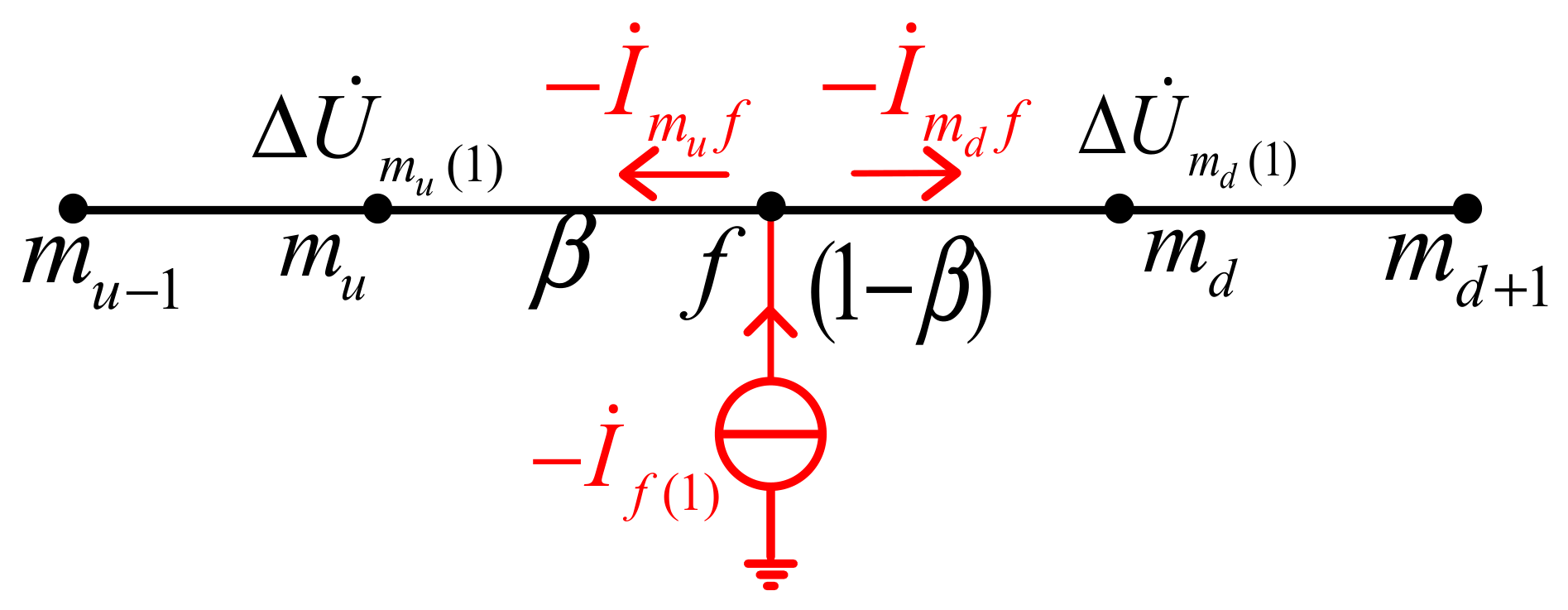
For a two-port network corresponding to a known measurement point section mu-md, as shown in Figure 7, the positive-sequence impedance of the line is denoted by $Z_{m_u{m}_d}$. After a fault occurs, the fault point f divides the line into two segments, muf and md f, whose length ratio is $\beta :1-\beta$.

After the fault occurs, the NPSVMD at the measurement nodes on both sides of the line is calculated according to the method described previously, as expressed in Equation (29).

$$\left\{\begin{array}{l}{D}_{m_u}=\left|\delta U_{m_u}\right|=\left|Z_{m_s{m}_u(1)}{\dot{I}}_{f(1)}\right|\\ D_{m_d}=\left|\delta U_{m_d}\right|=\left|Z_{m_{s}f(1)}{\dot{I}}_{f(1)}\right|\end{array}\right.$$

(29)

where $Z_{m_s{m}_u(1)}$ denotes the EPSI between the measurement point m_u and the reference node, and $Z_{m_{s}f(1)}$ denotes the EPSI between the fault location and the reference node.

Subtracting the two terms in Equation (29) yields:

$$\begin{array}{ll}{D}_{m_u}-D_{m_d}& =\left|\delta U_{m_u}\right|-\left|\delta U_{m_d}\right|\\ & =\left|Z_{m_s{m}_u(1)}{\dot{I}}_{f(1)}-Z_{m_{s}f(1)}{\dot{I}}_{f(1)}\right|\\ & =\left|{\dot{I}}_{f(1)}\left(Z_{m_s{m}_u(1)}-Z_{m_{s}f(1)}\right)\right|\\ & =\left|{\dot{I}}_{f(1)}{Z}_{m_{u}f(1)}\right|\end{array}$$

(30)

The NPSVMD at measurement nodes m_u and m_d, presented in Equations (29) and (30), are derived theoretically. In practice, both can be calculated from the NPSV and NPSC measurements acquired at each measurement point, as shown in Equation (31).

$$\left\{\begin{array}{l}\delta U_{m_u}={\displaystyle \sum _{i=1}^s\left(Z_{m_u{m}_i(1)}{\dot{I}}_{m_i(1)}^{\prime }-{\dot{U}}_{m_u(1)}^{\prime }\right)}\\ \delta U_{m_d}={\displaystyle \sum _{i=1}^s\left(Z_{m_d{m}_i(1)}{\dot{I}}_{m_i(1)}^{\prime }-{\dot{U}}_{m_d(1)}^{\prime }\right)}\end{array}\right.$$

(31)

Similarly, subtracting the two terms in Equation (31) yields:

$$\begin{array}{ll}{D}_{m_u}-D_{m_d}& =\left|\delta U_{m_u}\right|-\left|\delta U_{m_d}\right|\\ & =\left|\delta U_{m_d}-\delta U_{m_u}\right|\\ & =\left|{\displaystyle \sum _{i=1}^s\left((Z_{m_d{m}_i(1)}-Z_{m_u{m}_i(1)}){\dot{I}}_{m_i(1)}^{\prime }\right)}-\left({\dot{U}}_{m_d(1)}^{\prime }-{\dot{U}}_{m_u(1)}^{\prime }\right)\right|\end{array}$$

(32)

It can be inferred from Equations (30) and (32) that, for a given candidate fault location α, the NPSVMD calculated from the measurement data should be consistent with the theoretical value derived from the line parameters. Based on this, this paper constructs a distance function r(α) to characterize the degree of deviation between the two.

$$\begin{array}{ll}r(\alpha )& =\left|{\displaystyle \sum _{i=1}^s\left((Z_{m_d{m}_i(1)}-Z_{m_u{m}_i(1)}){\dot{I}}_{m_i(1)}^{\prime }-\left({\dot{U}}_{m_d(1)}^{\prime }-{\dot{U}}_{m_u(1)}^{\prime }\right)\right)}\right|-\left|{\dot{I}}_{f(1)}{Z}_{m_{u}f(1)}\right|\\ & =\left|{\displaystyle \sum _{i=1}^s\left((Z_{m_d{m}_i(1)}-Z_{m_u{m}_i(1)}){\dot{I}}_{m_i(1)}^{\prime }\right)}-\left({\dot{U}}_{m_d(1)}^{\prime }-{\dot{U}}_{m_u(1)}^{\prime }\right)\right|-\alpha \left|{\dot{I}}_{f(1)}{Z}_{m_u{m}_d(1)}\right|\end{array}$$

(33)

where 0 < α < 1.

For the true fault location, the theoretical calculation result most closely matches the measurement result; therefore, the distance estimation function attains its minimum value. The fault location can then be expressed as:

$$\alpha =\arg \underset{\alpha \in \left(0,1\right)}{\min }r(\alpha )$$

(34)

As can be seen from Equation (33) that, aside from the current and voltage information obtained from measurements and the line parameters, the fault current ${\dot{I}}_{f(1)}$ remains unknown in the distance estimation function. Therefore, it is necessary to seek a method for determining ${\dot{I}}_{f(1)}$.

The variation in the NPSV before and after the fault can be equivalently regarded as the voltage response caused by the injection of a current source at the fault point. Accordingly, measurement nodes m_u and m_d satisfy Equation (35).

$$\begin{array}{l}\Delta {\dot{I}}_{m_u(1)}={\displaystyle \sum _{i=1}^s{Y}_{m_{u}i(1)}\Delta {\dot{U}}_{i(1)}}\\ \Delta {\dot{I}}_{m_d(1)}={\displaystyle \sum _{i=1}^N{Y}_{m_{d}i(1)}\Delta {\dot{U}}_{i(1)}}\end{array}$$

(35)

where $\Delta {\dot{I}}_{m_u(1)}$ and $\Delta {\dot{I}}_{m_d(1)}$ denote the nodal current variations at measurement nodes m_u and m_d, respectively; $Y_{m_{u}i(1)}$ and $Y_{m_{d}i(1)}$ represent the positive-sequence mutual admittances between measurement point m_u, m_d and node i; and $\Delta {\dot{U}}_{i(1)}$ denotes the positive-sequence voltage variation at node i before and after the fault. Rearranging Equation (35) yields:

$$\begin{array}{ll}\Delta {\dot{I}}_{m_u(1)}={\displaystyle {\displaystyle \sum _{i=1}^s}{Y}_{m_{u}i(1)}\Delta {\dot{U}}_{i(1)}}=& {\displaystyle {\displaystyle \sum _{i\ne m_u,i\ne m_d}^s}-Y_{m_{u}i(1)}(\Delta {\dot{U}}_{m_u(1)}-\Delta {\dot{U}}_{i(1)}})+{\displaystyle {\displaystyle \sum _{i=1}^s}{Y}_{m_{u}i(1)}\Delta {\dot{U}}_{m_u(1)}}\\ & -Y_{m_u{m}_d(1)}(\Delta {\dot{U}}_{m_u(1)}-\Delta {\dot{U}}_{m_d(1)})\\ \Delta {\dot{I}}_{m_d(1)}={\displaystyle {\displaystyle \sum _{i=1}^N}{Y}_{m_{d}i(1)}\Delta {\dot{U}}_{i(1)}}=& {\displaystyle {\displaystyle \sum _{i\ne m_u,i\ne m_d}^N}-Y_{mi(1)}(\Delta {\dot{U}}_{m_d(1)}-\Delta {\dot{U}}_{i(1)}})+{\displaystyle {\displaystyle \sum _{i=1}^N}{Y}_{m_{d}i(1)}\Delta {\dot{U}}_{m_d(1)}}\\ & -Y_{m_d{m}_u(1)}(\Delta {\dot{U}}_{m_d(1)}-\Delta {\dot{U}}_{m_u(1)})\end{array}$$

(36)

The forward network model is shown in Figure 8. As can be seen from Figure 8, measurement nodes m_u and m_d also satisfy KCL:

$$\begin{array}{l}{\displaystyle {\displaystyle \sum _{i\ne m_u,i\ne m_d}^s}-Y_{m_{u}i}(\Delta {\dot{U}}_{m_u(1)}-\Delta {\dot{U}}_{i(1)}})+{\displaystyle {\displaystyle \sum _{i=1}^s}{Y}_{m_{u}i}\Delta {\dot{U}}_{m_u(1)}}-Y_{m_u{m}_d}(\Delta {\dot{U}}_{m_u(1)}-\Delta {\dot{U}}_{i(1)})/\beta =0\\ {\displaystyle {\displaystyle \sum _{i\ne m_u,i\ne m}^N}-Y_{mi}(\Delta {\dot{U}}_{m_d(1)}-\Delta {\dot{U}}_{i(1)}})+{\displaystyle {\displaystyle \sum _{i=1}^N}{Y}_{m_{d}i}\Delta {\dot{U}}_{m_d(1)}}-Y_{m_d{m}_u}(\Delta {\dot{U}}_{m_d(1)}-\Delta {\dot{U}}_{i(1)})/(1-\beta )=0\end{array}$$

(37)

where from left to right, the first part represents the sum of the currents flowing from the measurement point m_u (m_d) to its adjacent measurement nodes, excluding the measurement point m_u (m_d); the second part represents the shunt current to ground at the measurement point m_u (m_d); and the third part represents the current ${\dot{I}}_{m_{u}f}$(${\dot{I}}_{m_{d}f}$) flowing from the measurement point m_u(m_d) to the fault point f.

In summary, by eliminating the common terms in Equations (36) and (37), the following can be obtained:

$$\left\{\begin{array}{l}\Delta {\dot{I}}_{m_u(1)}=Y_{m_u{m}_d(1)}(\Delta {\dot{U}}_{m_u(1)}-\Delta {\dot{U}}_{f(1)})/\beta -Y_{m_u{m}_d(1)}(\Delta {\dot{U}}_{m_u(1)}-\Delta {\dot{U}}_{m_d(1)})\hfill \\ \Delta {\dot{I}}_{m_d(1)}=Y_{m_d{m}_u(1)}(\Delta {\dot{U}}_{m_d(1)}-\Delta {\dot{U}}_{f(1)})/(1-\beta )-Y_{m_d{m}_u(1)}(\Delta {\dot{U}}_{m_d(1)}-\Delta {\dot{U}}_{m_u(1)})\hfill \end{array}\right.$$

(38)

Meanwhile, the fault point f in Figure 4 also satisfies KCL, with the fault current flowing from the fault point to both sides:

$$\begin{array}{ll}-{\dot{I}}_{f(1)}& =-{\dot{I}}_{m_{u}f}-{\dot{I}}_{m_{d}f}=-Y_{m_u{m}_d}(\Delta {\dot{U}}_{m_u(1)}-\Delta {\dot{U}}_{f(1)})/\beta -Y_{m_d{m}_u}(\Delta {\dot{U}}_{m_d(1)}-\Delta {\dot{U}}_{f(1)})/(1-\beta )\\ & =-\left[\Delta {\dot{I}}_{m_u(1)}+Y_{m_u{m}_d(1)}(\Delta {\dot{U}}_{m_u(1)}-\Delta {\dot{U}}_{m_d(1)})+\Delta {\dot{I}}_{m_d(1)}+Y_{m_d{m}_u(1)}(\Delta {\dot{U}}_{m_d(1)}-\Delta {\dot{U}}_{m_u(1)})\right]\\ & =-\left(\Delta {\dot{I}}_{m_u(1)}+\Delta {\dot{I}}_{m_d(1)}\right)\end{array}$$

(39)

Simplifying yields:

$${\dot{I}}_{f(1)}=\Delta {\dot{I}}_{m_u(1)}+\Delta {\dot{I}}_{m_d(1)}$$

(40)

As shown in Equation (40), the fault current ${\dot{I}}_{f(1)}$ can be calculated equivalently by determining the change in current at the measurement nodes at both ends of the faulted line.

Substituting Equation (40) into Equation (33) yields:

$$\begin{array}{ll}r(\alpha )& =\left|{\displaystyle \sum _{i=1}^s\left(\left(Z_{m_d{m}_i(1)}-Z_{m_u{m}_i(1)}\right){{\dot{I}}^{\prime }}_{m_i(1)}-\left({{\dot{U}}^{\prime }}_{m_d(1)}-{{\dot{U}}^{\prime }}_{m_u(1)}\right)\right)}\right|-\left|{\dot{I}}_{f(1)}{Z}_{m_{u}f(1)}\right|\\ & =\left|{\displaystyle \sum _{i=1}^s\left(\left(Z_{m_d{m}_i(1)}-Z_{m_u{m}_i(1)}\right){{\dot{I}}^{\prime }}_{m_i(1)}-\left({{\dot{U}}^{\prime }}_{m_d(1)}-{{\dot{U}}^{\prime }}_{m_u(1)}\right)\right)}\right|-\alpha \left|{\dot{I}}_{f(1)}{Z}_{m_u{m}_d(1)}\right|\\ & =\left|{\displaystyle \sum _{i=1}^s\left(\left(Z_{m_d{m}_i(1)}-Z_{m_u{m}_i(1)}\right){{\dot{I}}^{\prime }}_{m_i(1)}-\left({{\dot{U}}^{\prime }}_{m_d(1)}-{{\dot{U}}^{\prime }}_{m_u(1)}\right)\right)}\right|-\alpha \left|\left(\Delta {\dot{I}}_{m_u(1)}+\Delta {\dot{I}}_{m_d(1)}\right)Z_{m_u{m}_d(1)}\right|\end{array}$$

(41)

Since the fault point is necessarily located within the identified faulted line segment m_u-m_d, the fault distance coefficient α must satisfy the sectional constraint. Based on this, the determination of the fault distance coefficient can be formulated as the following constrained optimization problem subject to 0 < α < 1:

$$\underset{\alpha }{\min }r(\alpha )=\underset{\alpha }{\min }\left|\left|{\displaystyle \sum _{i=1}^s\left(\left(Z_{m_d{m}_i(1)}-Z_{m_u{m}_i(1)}\right){\dot{I}}_{m_i(1)}^{\prime }-\left({\dot{U}}_{m_d(1)}^{\prime }-{\dot{U}}_{m_u(1)}^{\prime }\right)\right)}\right|-\alpha \left|\left(\Delta {\dot{I}}_{m_u(1)}+\Delta {\dot{I}}_{m_d(1)}\right)Z_{m_u{m}_d(1)}\right|\right|$$

(42)

To make the fault distance calculation procedure reproducible, the numerical implementation of Equation (42) is further described as follows.

The solution of the fault distance coefficient α in Equation (42) is essentially a one-dimensional bounded minimization problem over the interval (0,1). Since the candidate faulted measurement section m_u-m_d has already been identified in the preceding stage, the fault location does not need to be searched over the entire network. Instead, only the normalized position of the fault point within the identified measurement section needs to be determined.

In this paper, a two-stage deterministic search strategy is adopted to solve α. First, a coarse search is performed over the interval (0,1) with a step size of Δα₁ = 10⁻³, namely:

$${\alpha }_k=k\Delta {\alpha }_1,k=1,2,\cdots ,{\displaystyle \frac{1}{\Delta {\alpha }_1}}-1.$$

(43)

The value of r(α_k) is calculated for each candidate point, and the coarse optimal solution is obtained as:

$${\alpha }_c=arg\underset{{\alpha }_k\in (0,1)}{min}r({\alpha }_k)$$

(44)

Then, a refined local search interval is constructed around α_c, which can be expressed as:

$$\alpha \in [max(0,{\alpha }_c-\Delta {\alpha }_1),min(1,{\alpha }_c+\Delta {\alpha }_1)]$$

(45)

Within this local interval, a finer step size of Δα₂ = 10⁻⁵ is used to further search for the minimum of r(α). The final estimated fault distance coefficient is determined by:

$$\alpha \ast =arg\underset{\alpha \in [max(0,{\alpha }_c-\Delta {\alpha }_1),(1,{\alpha }_c+\Delta {\alpha }_1)]}{min}r(\alpha ).$$

(46)

The search process is terminated when the search resolution reaches the preset accuracy or when the variation between two successive estimates satisfies:

$$\mid {\alpha }^{(t)}-{\alpha }^{(t-1)}\mid <{10}^{-5}.$$

(47)

The obtained α represents the normalized fault location with respect to the identified measurement section m_u-m_d, rather than the relative position within the original physical line section.

From the computational perspective, the optimization in Equation (42) involves only one scalar variable. Each evaluation of r(α) requires only algebraic calculations using the measured voltage and current phasors, the known line parameters, and the equivalent fault current. No repeated power-flow calculation or large-scale matrix inversion is required. Therefore, the computational complexity is mainly determined by the number of search points. With the adopted search resolution, approximately 10³ function evaluations are required in the coarse search, while the refined search is conducted only in a small local interval around the coarse optimum. Since the search is performed only within the identified candidate measurement section, the computational burden is low, and the proposed distance estimation procedure is suitable for online or quasi-real-time implementation.

5.2. Steps for Distribution Network Fault Location with Limited Measurement Information

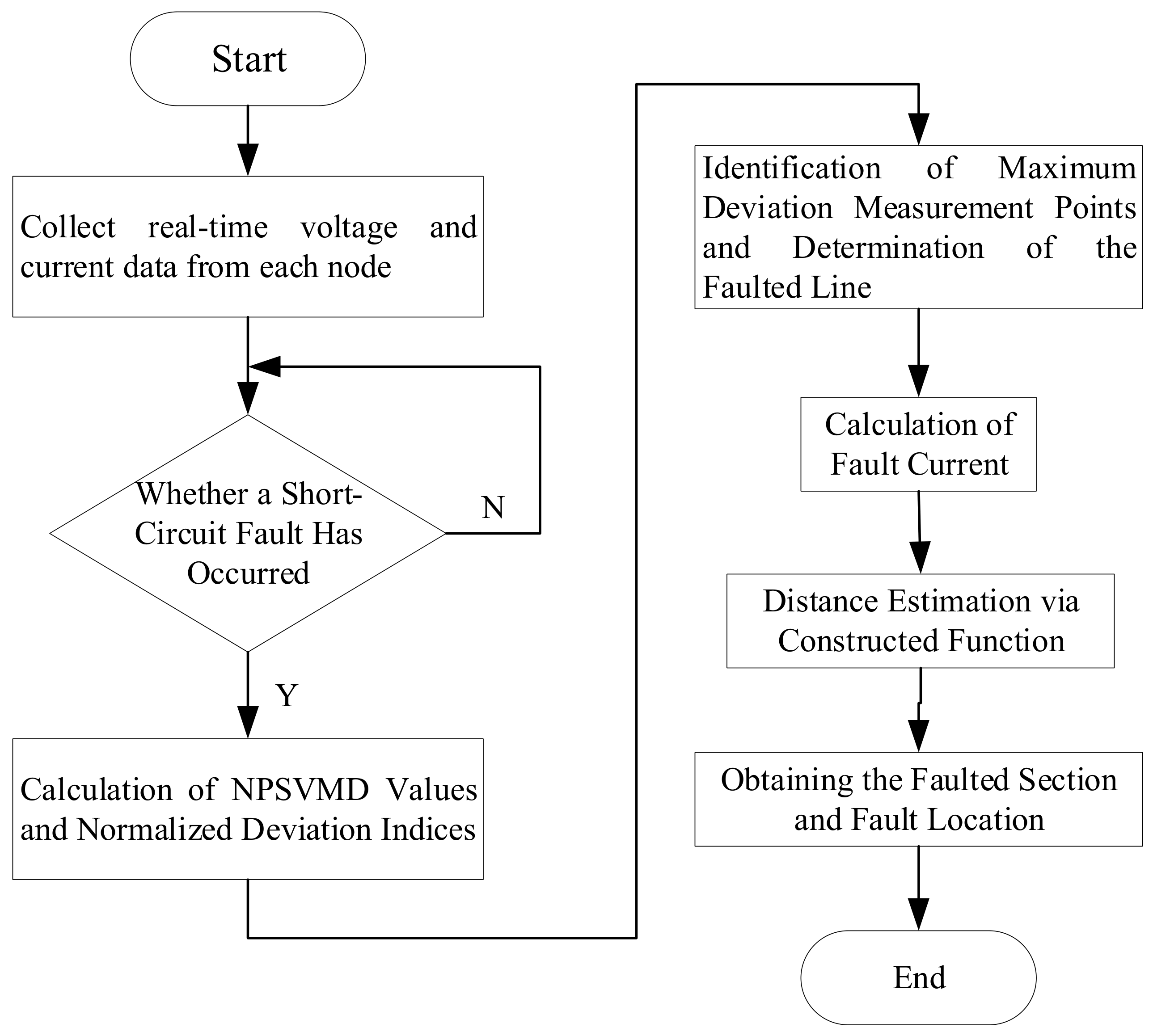
The fault location method adopted in this paper comprises four stages: fault detection, data preprocessing, fault section identification, and fault distance calculation. By continuously monitoring the NPSV and NPSC information of the distribution network, it is determined whether a fault has occurred in the system. Following a fault event, the pre-fault and post-fault measurement data are preprocessed to construct the magnitude of the NPSVMD, which is subsequently normalized. Based on the path relationship between the measurement point exhibiting the maximum NPSVMD and the reference node, the faulted line is identified. Finally, the fault current is equivalently derived using the NPSV variation equations at the measurement nodes located at both ends of the faulted line, and a distance estimation function is formulated by incorporating the NPSVMD values at these two measurement nodes, thereby achieving accurate fault location.

The flowchart of the distribution network fault location method based on limited measurement information is illustrated in Figure 9.

(1)

During system operation, the voltage and current data at each node are acquired in real time. Based on the collected nodal voltage and current information, a preliminary assessment is made to determine whether a short-circuit fault has occurred in the distribution network. When Equation (48) remains satisfied for a continuous period, the data windows corresponding to the pre-fault and post-fault intervals are recorded, and the subsequent fault location calculation process is initiated.

$$\left\{\begin{array}{l}\left|{\dot{U}}_i\right|\le U_{zd•i}\hfill \\ \left|{\dot{I}}_i\right|\ge I_{zd•i}\hfill \end{array}\right.$$

(48)

where ${\dot{U}}_i$ and ${\dot{I}}_i$ denote the measured voltage and current values at node i, respectively. The threshold values $U_{zd•i}$ and $I_{zd•i}$ can be selected based on practical conditions as $U_{zd•i}=(0.2~0.8)U_{N•i}$ and $I_{zd•i}=(1.2~1.5)I_{N•i}$, with $U_{N•i}$ representing the rated voltage at node i and $I_{N•i}$ representing the rated current at node i.

(2)

Select a data window during a period of stable system operation prior to the fault, and use its mean value as the reference NPSV ${\dot{U}}_{i(1)}$ before the node fault. After the fault occurs, select a short-term data window and use its mean value or the first stable phasor value as the NPSV ${\dot{U}}_{i(1)}^{\prime }$ after the fault.

(3)

Based on the impedance matrix of the distribution network and the directly measured NPSV and NPSC data, the NPSVMD and the normalized deviation index at each measurement point are calculated. Then the faulted line is identified by determining the common path among the unique paths from all measurement nodes exhibiting the maximum deviation to the reference source.

(4)

The fault current is calculated based on the change in NPSV at measurement nodes on both sides of the faulted line, and a distance-calculation function is constructed using the NPSVMD at these points, thereby enabling fault location and determining the exact fault position.

6. Simulation Verification and Analysis

This paper employs the IEEE 33-node standard distribution network model as a test case, with its topology illustrated in Figure 10. In accordance with the proposed principles for measurement device deployment, and to demonstrate the feasibility of the proposed method under limited measurement conditions, measurement devices are installed exclusively at the mandatory installation nodes. The corresponding node numbers that satisfy these criteria are: 0, 1, 2, 5, 17, 21, 24, and 32. The proportion of each section relative to the simplified line is presented in

Table 4. The proportion of each section to the simplified line.

Line	Section	${\mathit{\alpha }}_1$	${\mathit{\alpha }}_2$	Line	Section	${\mathit{\alpha }}_1$	${\mathit{\alpha }}_2$
1–2	1–2	0	1	2–5	2–3	0	0.2139
1–21	1–18	0	0.0559		3–4	0.2139	0.4366
	18–19	0.0559	0.5550		4–5	0.4366	1
	19–20	0.5550	0.7103	5–17	5–6	0	0.0545
	20–21	0.7103	1.0000		6–7	0.0545	0.1177
2–24	2–22	0	0.1932		7–8	0.1177	0.2247
	22–23	0.1932	0.5978		8–9	0.2247	0.3326
	23–24	0.5978	1.0000		9–10	0.3326	0.3500
5–32	5–25	0	0.0375		10–11	0.3500	0.3833
	25–26	0.0375	0.0900		11–12	0.3833	0.5408
	26–27	0.0900	0.3223		12–13	0.5408	0.6163
	27–28	0.3223	0.4978		13–14	0.6163	0.6830
	28–29	0.4978	0.5915		14–15	0.6830	0.7610
	29–30	0.5915	0.8170		15–16	0.7610	0.9423
	30–31	0.8170	0.8954		16–17	0.9423	1.0000
	31–32	0.8954	1.0000

.

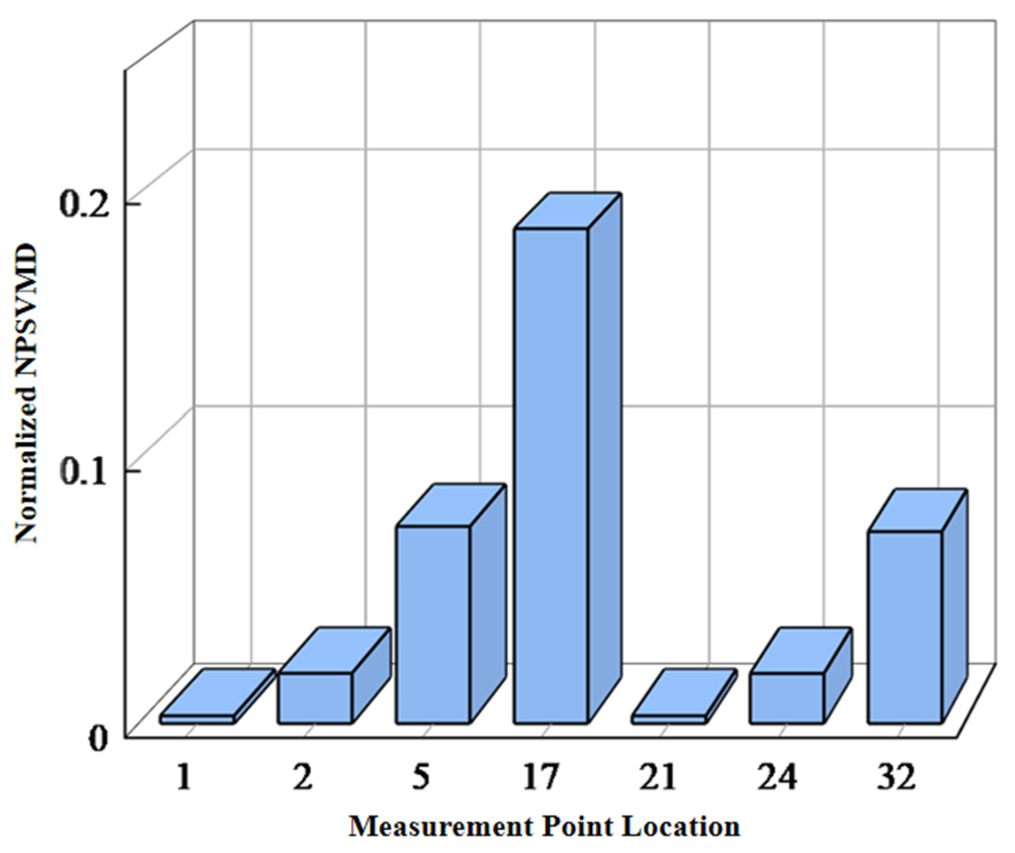
To better illustrate the principle and operational procedure of the fault location method proposed in this article, we will use the fault in the 9–10 section shown in Figure 10 as an example to provide a detailed explanation of the location process. The distance from the fault point to Node 9 accounts for 20% of the 9–10 section, which, after conversion, corresponds to 33.61% of the 5–17 line. The fault type is an AB-phase short circuit, with a ground resistance of 10 Ω. After the simulation run is completed, the NPSV and NPSC at each measurement point are extracted, and the NPSVMD at each measurement point is calculated. The results are presented in Figure 11.

As shown in Figure 11, the NPSVMD is greatest at measurement point 17, indicating that this point is located downstream of the fault. It is therefore inferred that the fault is located between lines 5 and 17. Next, a fault current distance function is constructed by calculating the change in forward-sequence voltage before and after the fault at measurement nodes 5 and 17 on either side of the line. Figure 8 shows the values of r(α) when 0 < α < 1.

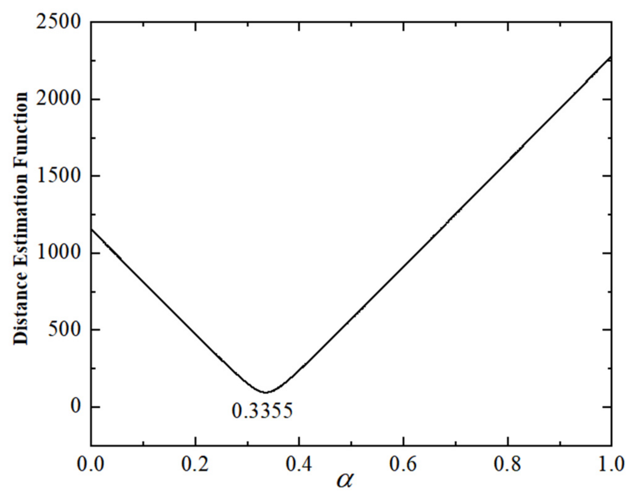
As shown in Figure 12, when the distance function is at its minimum, the corresponding fault distance coefficient is α = 0.3355. Referring to Table 1, it can be determined that the fault is located in the section 9–10 segment, with a localization error of 0.06%. To verify the accuracy and reliability of the method proposed in this article, the following section will test its localization performance under various fault conditions.

6.1. The Impact of Fault Locations

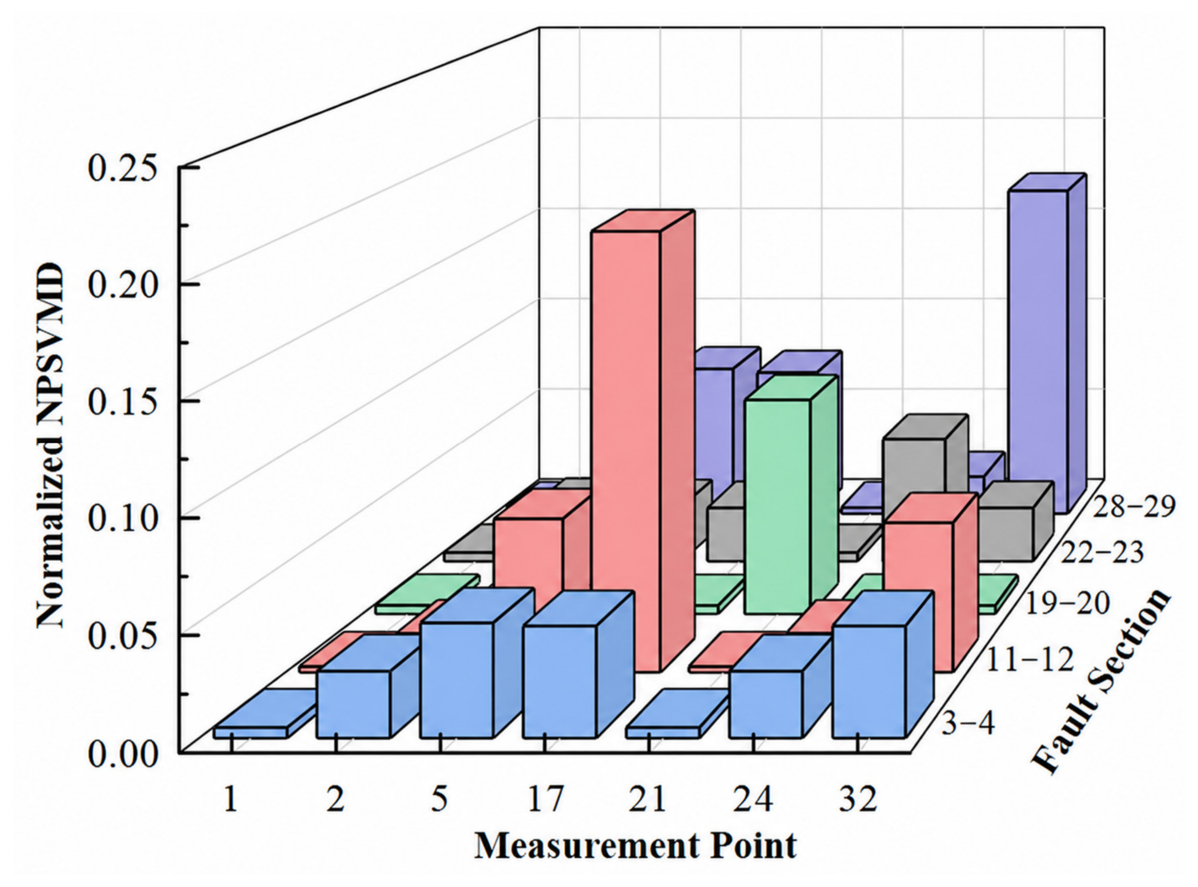
To evaluate the sensitivity of the proposed method to different fault locations, phase-A-to-phase-B short-circuit faults are set at 20% of the length of sections 3–4, 11–12, 19–20, 22–23, and 28–29, respectively, for testing purposes. The fault resistance is set to 10 Ω.

Figure 13 presents the processed results of D_i calculated from each set of experimental data. In the figure, the label “3–4” indicates that the fault occurs on section 3–4. Specifically, when the fault occurs on section 3–4, the NPSVMD values calculated at measurement nodes 5, 17, and 32 are equal and represent the maximum among all measurement nodes; therefore, it can be concluded that the fault is located on line 2–5. When the fault occurs on section 11–12, the NPSVMD calculated at measurement point 17 is the maximum among all measurement nodes; hence, the fault is identified as occurring on line 5–17. For the other test cases, the faulted line can also be accurately identified. Thus, the method proposed in this article remains effective for faulted line identification under different fault locations, even with a reduced number of measurement devices.

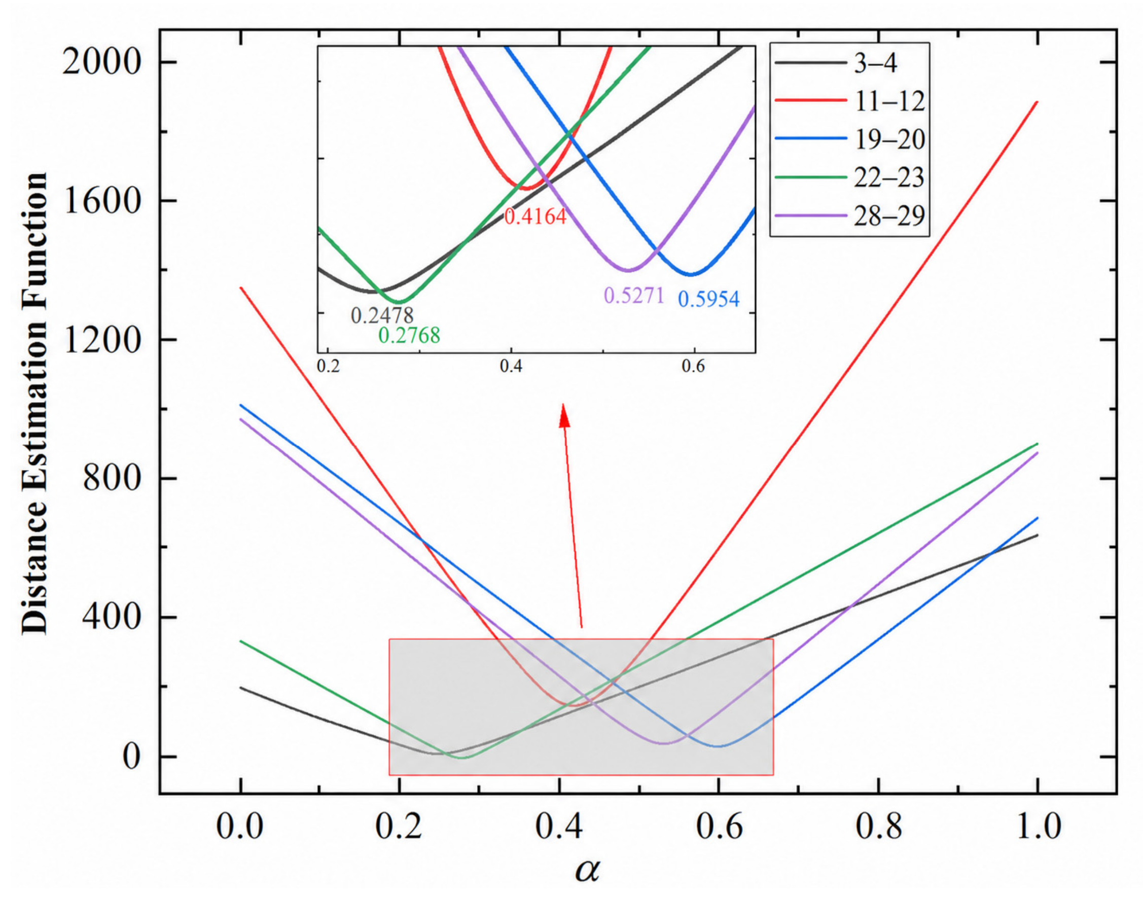
Next, by substituting the NPSV and NPSI data from each measurement point into the distance estimation function, the curves of r(α) under different fault locations can be obtained, as shown in Figure 14. It can be observed that in each test case, a value of α corresponding to the minimum of the distance estimation function can be identified, thereby enabling fault location in all scenarios.

By correlating the calculated fault distance coefficient with the data in Table 1, the specific faulted section for each test case can be determined. The location results and errors for the five test cases are shown in

Table 5. Positive sequence voltage measurement deviation at different fault locations.

Fault Section	Located Section	Set Fault Location	Identified Location	Location Error
3–4	3–4	0.2584	0.2478	1.06%
11–12	11–12	0.4148	0.4164	0.16%
19–20	19–20	0.5861	0.5954	0.93%
22–23	22–23	0.2741	0.2768	0.27%
28–29	28–29	0.5165	0.5271	1.05%

.

The results indicate that the method proposed in this article is capable of effectively locating faults in the tested sections of the distribution network.

6.2. The Impact of Equipment Measurement Errors

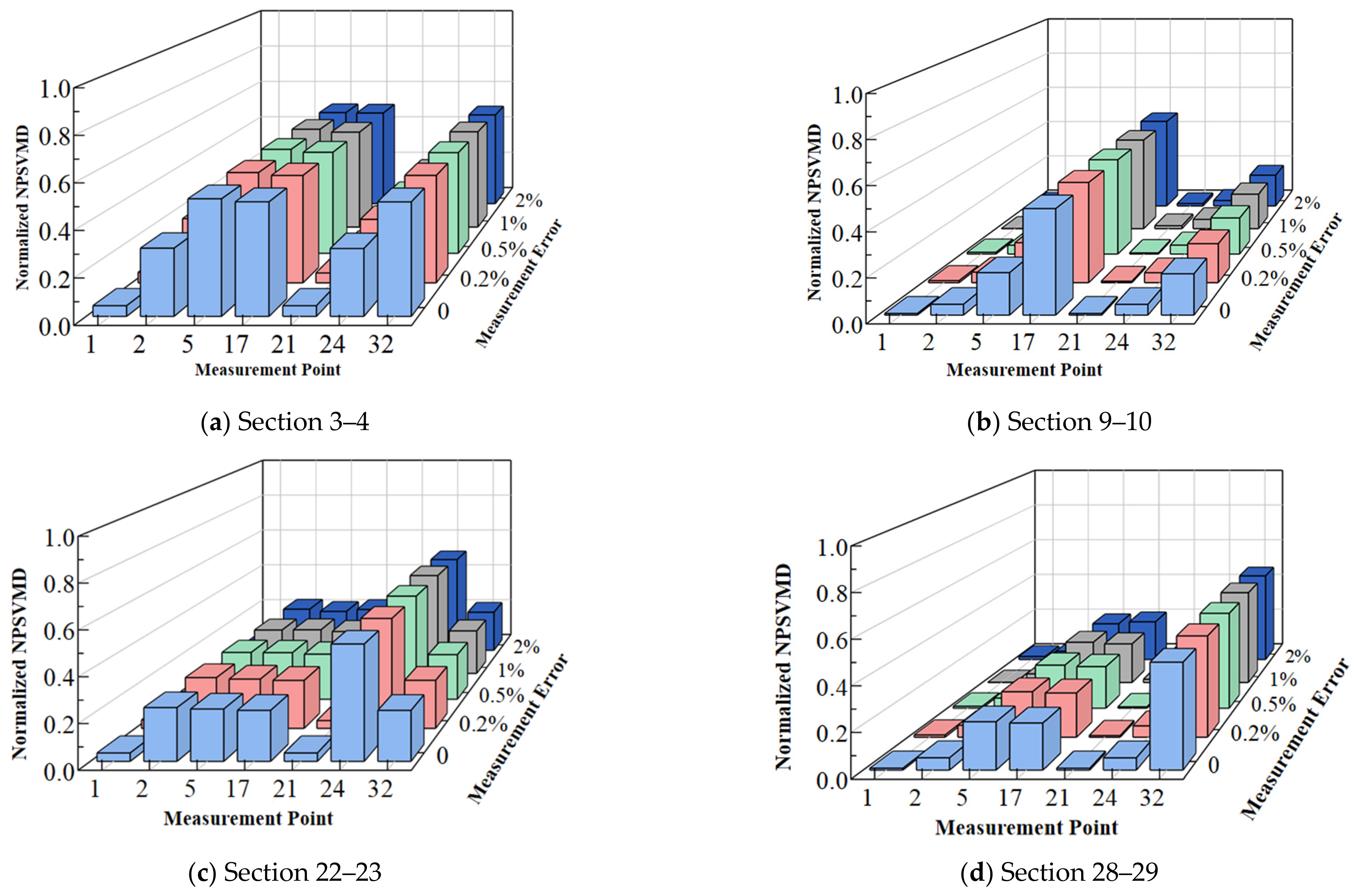
As indicated by the preceding analysis, measurement data from μPMU-type devices are typically subject to certain errors due to environmental interference and inherent limitations in measurement device accuracy. The magnitude error can generally be controlled within 0.5%. To evaluate the robustness of the proposed method in the presence of measurement errors, fault cases with a fault resistance of 10 Ω occurring at 20% of the length of sections 3–4, 9–10, 22–23, and 28–29 are selected as examples. Errors of 0.2%, 0.5%, 1%, and 2% are deliberately introduced into the measurement data at each node, and a condition without error is established as a reference for comparison, thereby enabling a systematic analysis of the method’s applicability. First, the NPSVMD at each measurement point is calculated based on the processed voltage and current data, as shown in Figure 15.

It can be observed from Figure 15 that as the measurement error increases, the normalized NPSVMD values at the respective measurement nodes exhibit relatively minor variations, and a maximum NPSVMD value is consistently present across all cases, enabling the identification of the faulted line 5–17. Moreover, when the fault occurs on section 3–4, multiple measurement nodes are located downstream of the fault, and it can still be observed that the NPSVMD values at several measurement nodes are approximately equal and represent the maximum. Therefore, the line identification principle proposed in this article demonstrates good applicability to measurement errors.

Next, the value of α is calculated at which the distance-to-fault function reaches its minimum in each test group and compared with the proportion of the faulted section relative to the corresponding line. The specific fault location results are shown in

Table 6. Positioning results under different measurement errors.

Fault Section	Measurement Error/%	Algorithm-Based Location	Standard Section	Locating the Faulted Area	Relative Fault Location Error/%
3–4	0	0.2501	(0.2154,0.4397)	3–4	0.83
	0.2	0.2483		3–4	1.01
	0.5	0.2580		3–4	0.04
	1	0.2638		3–4	0.54
	2	0.2475		3–4	1.10
9–10	0	0.3366	(0.3274,0.3443)	9–10	0.05
	0.2	0.3356		9–10	0.05
	0.5	0.3311		9–10	0.50
	1	0.3331		9–10	0.30
	2	0.3691		9–10	3.31
22–23	0	0.2770	(0.1933,0.5977)	22–23	0.28
	0.2	0.2739		22–23	0.02
	0.5	0.2825		22–23	0.84
	1	0.2935		22–23	1.94
	2	0.2750		22–23	0.09
28–29	0	0.5280	(0.5010,0.5942)	28–29	1.15
	0.2	0.5273		28–29	1.07
	0.5	0.5171		28–29	0.05
	1	0.5266		28–29	1.01
	2	0.5571		28–29	4.05

. The results indicate that as the measurement error increases, the location error exhibits a certain degree of increase, yet the overall error magnitude remains at a relatively low level. It is noteworthy that when the measurement error increases from 1% to 2%, the relative error of the fault distance calculation undergoes a significant abrupt change. However, given that the measurement error of μPMUs can be maintained within 1% under various operating conditions, the method proposed in this article demonstrates strong robustness even with limited measurement information when μPMUs are employed.

6.3. The Impact of Data Synchronization Errors

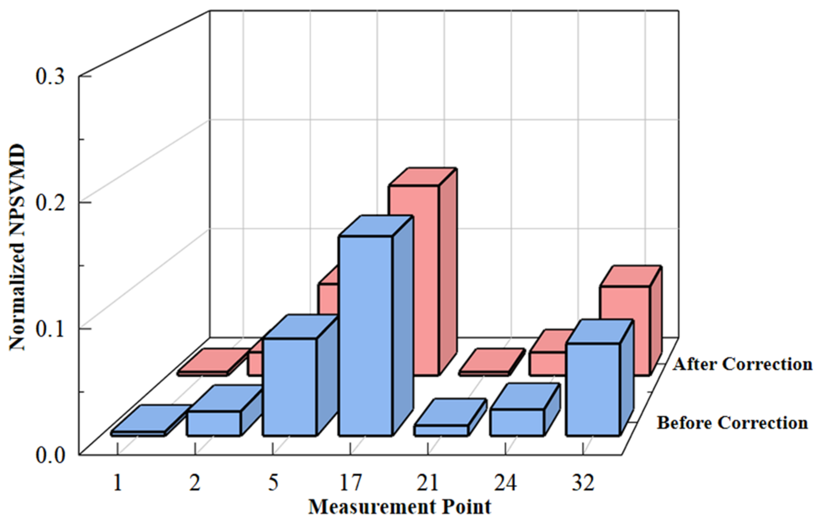
To evaluate the impact of synchronization error on the distance estimation performance of the proposed method, different types of faults are set at 20% of the length of section 8–9, with a fault resistance of 10 Ω. A synchronization error within the range of 0–1° is deliberately introduced into the phase angle of the electrical quantities measured at each node. Taking a two-phase short-circuit fault as an illustrative example, the difference in the NPSVMD before and after synchronization error correction is shown in Figure 16.

It can be seen that the relative magnitudes of the NPSVMD values at the respective measurement nodes remain unchanged before and after synchronization error correction. The measurement point corresponding to the maximum NPSVMD value is measurement Point 17, and its immediate upstream measurement point is measurement Point 5. Consequently, the fault is identified as being located on line 5–17, and the faulted line can be correctly identified in accordance with the faulted line identification principle.

Next, we will calculate the value of α at which the distance function reaches its minimum in each test group and compare it with the proportion of the actual fault location relative to the corresponding line. The specific results of the fault location are shown in

Table 7. Positioning results before and after correction of synchronization error.

Fault Type	Section Location	Distance Estimation Error Before Correction	Distance Estimation Error After Correction
AB	8–9	1.11%	0.61%
ABG	8–9	1.04%	0.61%
ABC	8–9	0.86%	0.61%

.

As shown in Table 7, synchronization errors have a significant impact on the location of two-phase short-circuit faults, but a relatively minor impact on other fault types. However, after processing using the self-synchronization correction method proposed in this paper, accurate fault location can be achieved for all types of faults. Therefore, under the synchronization measurement accuracy conditions of μPMU-type measurement devices, the method proposed in this article can achieve relatively accurate fault location.

6.4. The Impact of Distributed Energy Resources on the Grid

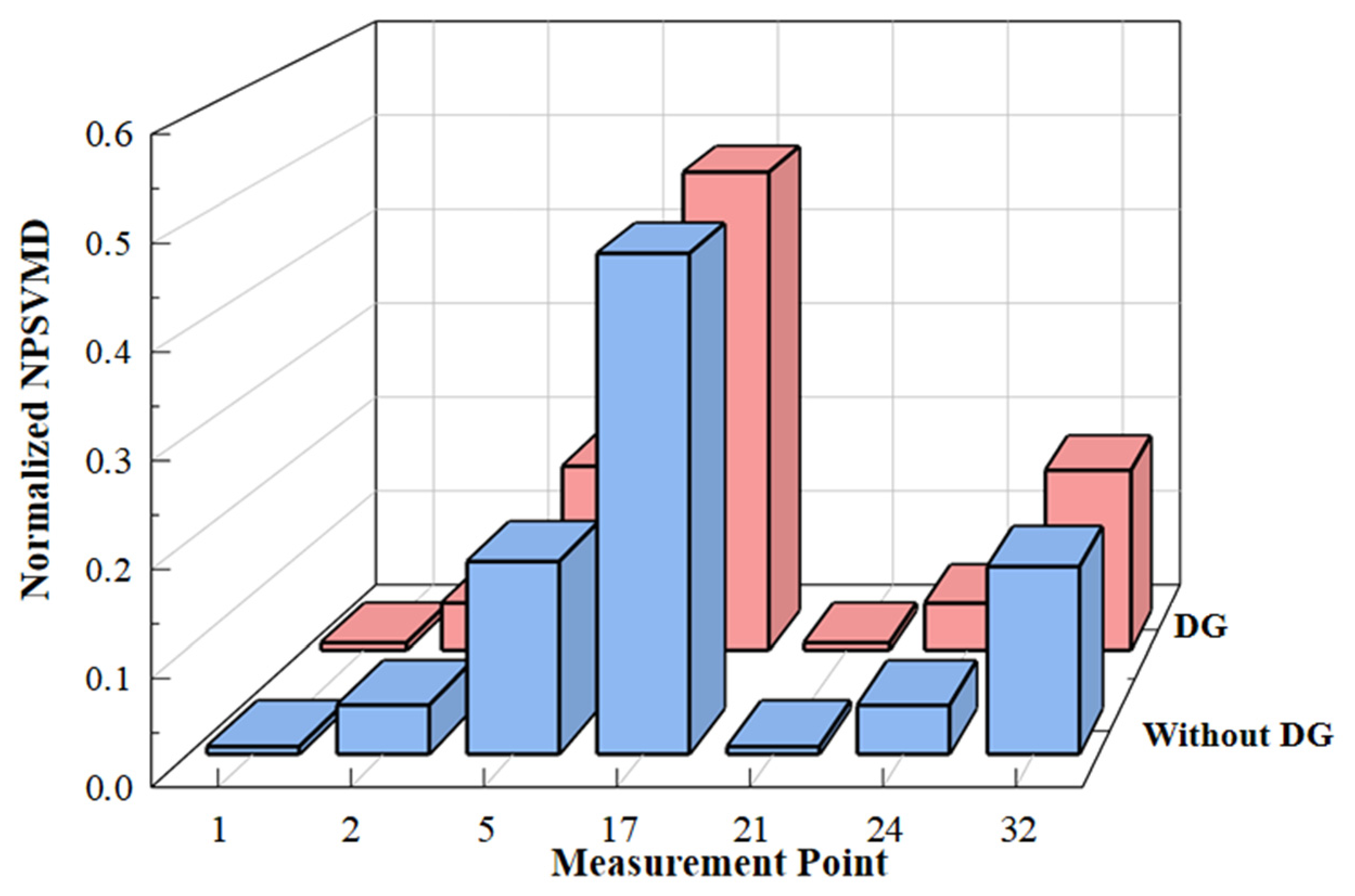
With the increasing penetration of complex active elements such as photovoltaic-electric vehicle microgrids in modern power systems [23], it is necessary to verify whether the proposed positioning method based on limited measurement information is affected by the integration of distributed generation (DG). Photovoltaic power sources with a capacity of 1 MW were connected at nodes 17 and 32. Taking a phase-to-phase short-circuit fault between phases A and B occurring at the 20% mark of the 10–11 section as an example, and using the same fault location without DG as a control test, D_i was calculated and normalized for each case. The results are shown in Figure 17.

After connecting to the DG, although the absolute values of the NPSVMD changed, the NPSVMD at measurement point 17 remained the largest among all measurement nodes. Therefore, it can be determined that the fault is located on line 5–17. Further calculation using the fault location equation yielded a fault distance coefficient of α = 0.350586641. Referring to Table 1, the fault is located in section 10–11, with a location error of 0.61%.

To verify the applicability of the fault location method proposed in this article under DG integration conditions, phase-A-to-phase-B short-circuit faults are separately set at 20% of the length of each section in the IEEE 33-node distribution network. The same fault locations without DG integration are used as control tests for comparison. The fault location results with and without DG integration are compared, as presented in

Table 8. Positioning results before and after DG access.

DG Integration Status	Correct Location Count	Incorrect Location Count	Average Distance Estimation Error
Not Connected	31	0	1.25%
Connected	31	0	2.56%

. The results indicate that after the integration of photovoltaic (PV) sources into the distribution network, the average location error increases from 1.25% to 2.56%, demonstrating that the impact of PV integration on the proposed method is relatively minor.

6.5. The Impact of Line Impedance Uncertainty and Topology Error

The proposed method relies on the pre-fault PSIM and the corresponding network topology. In practical distribution networks, however, line impedance parameters may deviate from their nominal values due to conductor temperature variations, aging effects, inaccurate line length records, and errors in engineering parameter databases. Therefore, it is necessary to evaluate the influence of line impedance uncertainty on the proposed fault location method.

To analyze the sensitivity of the proposed method to line parameter uncertainty, random perturbations were introduced into the positive-sequence impedance of each line section. The perturbed impedance can be expressed as:

$$z_{ij}^{\prime }=z_{ij}(1+{\epsilon }_{ij})$$

(49)

where z_ij is the nominal positive-sequence impedance of line section i−j, z_ij′ is the perturbed impedance used in the location calculation, and ε_ij is the relative impedance error. In the simulation, ε_ij was randomly generated within [−10%,10%] to represent different levels of parameter uncertainty. AB-phase short-circuit faults with a transition resistance of 10 Ω are set at 20% of the line length in section 9–10. The NPSVMD distribution and fault location results under different impedance deviation levels are obtained and compared with those under the ideal condition, and the specific data are shown in

Table 9. Fault location results under line impedance parameter deviations.

Line Impedance Systematic Error	Identified Measurement Section	$\mathbf{\alpha }$	Located Section	Relative Fault Location Error
0% (basic)	5–17	0.3355	9–10	0.05%
+2%	5–17	0.3381	9–10	0.20%
+5%	5–17	0.3435	9–10	0.74%
+10%	5–17	0.3521	10–11	1.60%
−2%	5–17	0.3338	9–10	0.23%
−5%	5–17	0.3291	8–9	0.70%
−10%	5–17	0.3185	8–9	1.76%

.

As shown in Table 9, under different line impedance parameter deviations, the proposed method can consistently identify the faulted measurement section as 5–17. This indicates that the impedance parameter deviation does not significantly change the relative distribution of the maximum NPSVMD measurement nodes, and the faulted measurement-section identification remains stable. However, as the impedance deviation increases, the estimated distance coefficient gradually deviates from the actual value, indicating that line parameter errors directly affect the minimum point of the distance function r(α) and thus influence the fault distance calculation accuracy.

It should be noted that the normalized interval corresponding to section 9–10 within the measurement section 5–17 is relatively narrow, and the preset fault location α = 0.3361 is close to the boundary of adjacent sections. Therefore, when the impedance deviation increases to +10%, −5%, or −10%, the estimated α crosses the boundary of adjacent physical sections and is mapped to section 10–11 or 8–9. Nevertheless, the relative fault location error remains within 2%, indicating that the proposed method has acceptable adaptability to line impedance parameter deviations within a certain range. Overall, line impedance errors mainly affect the accuracy of fault distance calculation, while their influence on faulted measurement-section identification is relatively limited.

Topology errors have a more fundamental influence on the proposed method than line impedance errors. The proposed faulted line identification principle is based on the unique path property of radial distribution networks. If the actual switch status or feeder topology is inconsistent with the pre-fault network model used for calculation, the common path extracted from the model may deviate from the actual electrical path. In this case, the maximum NPSVMD measurement nodes may be mapped to an incorrect candidate section, which may cause faulted line misidentification. Therefore, the proposed method requires that the pre-fault topology model be consistent with the actual operating topology during the fault location time window.

In practical implementation, this requirement can be satisfied by integrating the proposed method with the distribution automation system, supervisory control and data acquisition system, or feeder terminal units, so that the switch status and network topology can be updated before the fault location calculation. In addition, topology consistency checking can be performed using the measured voltage and current phasors before applying the proposed algorithm. Once topology inconsistency is detected, the network model should be updated before constructing the impedance matrix and performing the common path search.

In summary, line impedance uncertainty mainly affects the accuracy of fault distance calculation, while severe topology errors may affect the correctness of faulted line identification. Therefore, the proposed method is robust to moderate line parameter uncertainty but requires a reliable and updated pre-fault topology model. Improving online parameter identification and topology verification will be considered in future work to further enhance the engineering applicability of the proposed method.

7. Conclusions

To address the difficulties of full-coverage measurement deployment and the limited availability of fault information in practical distribution networks, this paper proposes a fault location method based on limited measurement information. The proposed method takes the node positive-sequence voltage measurement deviation (NPSVMD) as the key feature. By analyzing the spatial distribution characteristics of NPSVMD after a fault occurs, a faulted section identification principle based on the common-path property between the maximum-deviation measurement nodes and the reference node is established. Furthermore, the fault current is equivalently derived using the nodal voltage variation equations, and a distance estimation function is constructed to determine the fault location. The main conclusions are summarized as follows.

(1)

Based on the unique-path property of radial distribution networks, this paper proves that, under the assumptions of a single-source radial network, a single short-circuit fault, and non-negative line positive-sequence impedances, the NPSVMDs of the nodes located downstream of the fault point are theoretically identical and attain the maximum value. In contrast, the NPSVMDs of upstream nodes and lateral-branch nodes are relatively smaller. This property provides a clear theoretical basis for faulted section identification under limited measurement conditions, rather than relying only on observations from a specific example.

(2)

For practical engineering scenarios in which only a limited number of μPMUs can be installed, a faulted line identification and distance estimation method based on key measurement nodes is developed. The proposed method does not require measurement devices at all network nodes. Instead, equivalent measurement sections are formed using a small number of critical measurement nodes, and the candidate faulted section is determined by extracting the common path of the maximum NPSVMD measurement-point set. In addition, the fault distance coefficient α is formulated as a one-dimensional bounded minimization problem over the interval (0,1). Each function evaluation only involves algebraic calculations using measured phasors, line parameters, and the equivalent fault current. No repeated power-flow calculation or large-scale matrix inversion is required, indicating low computational complexity and potential for online implementation.

(3)

Simulation results on the IEEE 33-node distribution system demonstrate that the proposed method can effectively identify the faulted measurement section and further map the estimated fault location to the corresponding physical line section with only a limited number of measurement nodes. The effectiveness and robustness of the proposed method are verified under different fault locations, equipment measurement errors, data synchronization errors, and distributed generation integration. In particular, after synchronization error correction, the fault distance calculation accuracy is improved, which indicates that the proposed method can adapt to practical μPMU measurement environments with certain error disturbances.

(4)

From the perspective of engineering application, the proposed method achieves a favorable balance between measurement cost and fault location performance. It has clear physical interpretability, lightweight computation, and no dependence on training samples, making it suitable for fault location in distribution networks with sparse measurements and complex structures.

(5)

Future work will focus on the following aspects: first, incorporating online parameter identification to improve the adaptability of the method to line parameter uncertainty caused by conductor temperature variation, aging effects, and inaccurate parameter records; second, developing adaptive fault location strategies under dynamic topology and network reconfiguration conditions; third, integrating multi-source measurements and advanced state estimation techniques to enhance robustness under communication delays, data packet loss, and partial loss of key measurement nodes; and fourth, extending the validation framework from offline simulation to hardware-in-the-loop testing platforms or field measurement data, so as to further verify the engineering applicability of the proposed method in practical distribution networks.