Energy-Efficient Topology Optimization of Wireless Sensor Networks Using a Modified Genetic Algorithm

Abstract

This paper addresses the challenge of WSN topology optimisation through the development and implementation of a modified genetic algorithm (MGA). Unlike classical approaches, the proposed method is based on the assessment of sensor node distribution density, employing an adaptive penalty system and considering the minimum inter-node distance to determine optimal configurations during the evolutionary selection process. A software module has been developed in Python (version 3.12.1) for the simulation of WSN functionality, accounting for dynamic topology changes and limited network resources. A comparative analysis of the proposed approach’s effectiveness was conducted against greedy, random, and uniform algorithms, varying sensor ranges (20, 30 and 40 m) and minimum inter-node distance constraints. Simulation results for scenarios involving 25 and 100 sensor nodes demonstrate that the proposed MGA consistently outperforms traditional approaches, including uniform (mesh), greedy, and random search algorithms. Unlike these methods, which either result in significant overlap (up to 13.23%) or fail to deploy all nodes, the MGA achieves 100% node placement with near-zero overlap. Furthermore, the proposed method exhibits stable convergence and high reliability, maintaining consistent performance across multiple runs with diverse initial conditions. The proposed Integrated Energy Efficiency Metric (IEEM) establishes a relationship between the spatial distribution of sensor nodes and the overall energy consumption of a WSN. By linking topology formation with energy costs, this metric enables a comprehensive assessment of deployment efficiency. Simulation results across various deployment scenarios demonstrate that the proposed MGA consistently achieves the lowest IEEM values compared to Mesh, Greedy, and Random placement strategies. The observed improvements range from 4.76% to 31.38%, confirming a substantial reduction in total energy losses. The proposed approach is particularly well-suited for dense deployments and resource-constrained environments, where effective coverage and minimal energy consumption are critical.

1. Introduction

The rapid expansion of WSNs within the Internet of Things paradigm has fundamentally transformed data collection approaches in environmental monitoring, smart agriculture, and infrastructure security systems. However, the operational efficiency of such networks remains constrained by the finite energy resources of individual sensor nodes [1,2]. Since radio communication typically accounts for the largest share of total power consumption, the spatial configuration of the network—its topology—is a critical factor influencing the system’s “lifetime”. Optimised node placement not only ensures maximum area coverage but also minimises the power required for multi-hop data transmission by maintaining rational inter-node distances.

Achieving a balance between integral coverage and energy conservation remains a challenging task, particularly in heterogeneous environments [3]. Random deployment often results in “coverage holes” or excessive node clustering, leading to rapid battery depletion in high-traffic zones (the “energy hole” problem). The problem of optimal sensor node placement belongs to the class of NP-hard combinatorial optimisation tasks, as it requires the simultaneous consideration of multiple interdependent criteria: maximising study area coverage, ensuring full or k-connectivity of the network, maintaining minimum inter-node distances, and accounting for sensing ranges and limited energy resources. The task becomes particularly complex when integrating new nodes into an existing topology, where a balance between deployment density and energy load uniformity must be preserved.

Traditional optimisation methods often fail to cope with the NP-hard nature of large-scale WSN deployment tasks. Metaheuristic approaches, specifically Genetic Algorithms (GAs), have proven to be powerful tools for exploring complex solution spaces. Analysis of scholarly works in the field of evolutionary WSN topology optimisation [4,5,6,7,8,9] indicates the widespread use of multi-objective genetic algorithms to resolve the trade-off between coverage area and energy efficiency. However, most known solutions (particularly those based on Pareto optimisation) are characterised by high computational complexity, limiting their real-time application for large node arrays.

Furthermore, a significant portion of existing multi-objective approaches focuses on optimising the network’s integral characteristics (such as total coverage or average energy efficiency), often ignoring the local spatial correlation between neighbouring nodes. This leads to zones with critically high device density, provoking excessive interference and uneven energy depletion within individual clusters.

To address these issues, this paper proposes an approach for sensor node placement based on a modified genetic algorithm to minimise redundant overlap across various sensing ranges on a plane. The primary contribution of this research is the development of a modified genetic algorithm that evaluates the distribution density of sensor nodes using constraints and minimum inter-node distances to determine optimal configurations during the evolutionary selection process.

The paper is structured as follows. Section 2 reviews existing works dedicated to the optimisation of sensor node deployment using evolutionary and bio-inspired algorithms. Section 3 presents the author’s approach for optimal sensor node placement based on the modified genetic algorithm. Section 4 provides flowcharts of the existing approaches (uniform, greedy, and random search) selected for comparison with the author’s method. Section 5 presents the results of experimental studies on stochastic sensor node deployment with variable sensing ranges (20, 30, and 40 m) and corresponding adjustments to minimum inter-node distance constraints. Section 6 concludes the study and outlines directions for future research.

2. Related Works

The operational efficiency of a WSN largely depends on its spatial deployment strategy, as the network topology directly determines energy consumption, communication reliability, and monitoring quality. Contemporary research emphasises that radio transmission is the most energy-intensive process in a sensor’s life cycle. Thus, forming an optimal topology is not merely a matter of ensuring the necessary area coverage, but also a task of minimising inter-node interference and eliminating redundant sensing overlap. The latter factor is critical: overlapping coverage zones lead to data duplication and irrational use of energy resources, thereby reducing the overall network “lifetime”. Since finding optimal coordinates for sensor placement to maximise coverage with minimal energy expenditure is an NP-hard problem, traditional gradient-based methods are increasingly being replaced by metaheuristic approaches. In recent years, researchers have focused on evolutionary and bio-inspired algorithms capable of efficiently processing multidimensional solution spaces and finding trade-offs between conflicting design objectives.

Paper [10] addresses the problem of ensuring stable monitoring point coverage in WSNs while minimising energy consumption. The central contribution is the development of an Improved Grey Wolf Optimiser (IGWO), aimed at overcoming the premature convergence issues characteristic of standard evolutionary methods. The authors modified the algorithm by implementing a “best point set” method for more rational population initialisation, alongside a non-linear convergence strategy and adaptive mutation mechanisms. This allows the algorithm to avoid local extrema more effectively during the search for optimal coordinates. Experimental studies, conducted using a mathematical energy consumption model, confirmed the superiority of the IGWO method over classical genetic algorithms and Flower Pollination Algorithms (FPA).

Article [11] solves the problem of relay node placement optimisation in WSNs. The authors introduced an Improved Genetic Algorithm for Relay Node Deployment (IGA-RNDP), which effectively tackles node placement in complex network environments where traditional methods suffer from local extrema and slow convergence rates. The study describes the integration of an elitist preservation mechanism and an enhanced search strategy, allowing the algorithm to maintain high population diversity and find sub-optimal solutions more rapidly. Experimental testing of the IGA-RNDP algorithm against existing optimisation methods demonstrated high performance in terms of processing speed and topology quality.

The authors of [12] developed a modified algorithm based on the Bron-Kerbosch method (MBK-SD), integrating graph theory with computational geometry. In the first stage, the algorithm models target objects as graph vertices, where edges denote the possibility of joint coverage by a single sensor. The use of a modified maximum clique search allows targets to be grouped into optimal clusters. In the second stage, an iterative circle intersection method is implemented to mathematically determine precise sensor coordinates, ensuring the maximum number of objects is covered within the sensing range. Comparative analysis with existing heuristic and greedy algorithms confirmed the advantage of the MBK-SD method: the approach demonstrated the ability to provide 100% target coverage using significantly fewer active devices.

Paper [13] presents an approach for WSN deployment in complex heterogeneous environments, considering the stochastic nature of radio wave propagation, particularly Rayleigh fading effects. A mathematical framework was developed to minimise total network energy consumption while ensuring that the probability of communication outage on each link remains below a specified critical threshold. The authors account for both large-scale path loss and small-scale signal fluctuations caused by multi-path propagation. A key feature is the inclusion of the exponential dependence of transmission power on data rates, making the algorithm adaptive to specific application requirements. Simulation results confirmed that accounting for failure probability during topology planning leads to substantial energy savings compared to existing heuristic methods.

In [14], the application of a modern metaheuristic algorithm—the Nutcracker Optimiser (NO)—is considered. This algorithm mimics the complex behaviour of birds during food searching and storage to minimise localization errors for unknown nodes in a WSN structure. The primary contribution lies in adapting NO strategies (searching, collecting, and spatial orientation) for the iterative refinement of node coordinates based on anchor (reference) point data. The methodology involves using inter-node distances to formulate a fitness function, which the algorithm optimises by simulating two main behavioural phases: cache laying and subsequent retrieval. This enables the system to effectively avoid local optima, a typical problem for classical localization methods, ensuring high accuracy even in noisy data environments. The effectiveness of the approach was validated through experiments in a specific geospatial scenario in Istanbul. Comparative analysis with well-known algorithms, such as Particle Swarm Optimisation (PSO) and Artificial Bee Colony (ABC), demonstrated a significant advantage for the NO method in terms of root mean square error and convergence speed.

The authors in [15] introduced the application of graph theory concepts, specifically the Grundy number, to precisely determine the minimum required number of sensors and their optimal spatial coordinates in complex three-dimensional landscapes. The primary contribution of the work is the development of a deterministic Grundy Number-based Deployment algorithm (GN-DSD) that addresses the Q-coverage problem. Unlike stochastic methods, this algorithm analyses the spatial coordinates of targets and constructs an adjacency graph, where the Grundy number calculation allows for the identification of independent sets of objects for efficient coverage. To ensure stable network connectivity, the authors further proposed a relay node placement method based on the Breadth-First Search (BFS) algorithm, guaranteeing seamless transmission of collected data to the base station. The effectiveness of the proposed approach was validated through a series of simulations, demonstrating its ability to minimise the number of nodes utilised while maintaining a specified level of coverage reliability. Comparison with existing evolutionary methods showed the superiority of the developed solution in reducing computational complexity and eliminating sensor redundancy.

Work [16] is dedicated to the Dynamic Multi-Packet Adaptive Grey Wolf Optimiser (DMPA-GWO++), specifically designed for the rapid recovery of network connectivity and coverage following cascading device failures. A fundamental feature of the proposed approach is the division of the algorithm’s population into several independent “packs”, which significantly expands the search space for optimal solutions and prevents premature stagnation of the computational process. The DMPA-GWO++ model integrates adaptive control parameters that dynamically adjust the topology restoration trajectory depending on the number of lost nodes and the priority of monitoring zones. This ensures intelligent network reconfiguration, where the new coordinates of active elements are calculated considering the minimisation of energy consumption for data forwarding under altered conditions. Practical validation of the method in a smart farm environment demonstrated its high efficiency in restoring IoT infrastructure functionality compared to standard versions of evolutionary algorithms.

The authors in [17] presented an enhanced global optimisation and deployment strategy for WSNs—the Multi-strategy Exchange Demand-Supply Optimiser (MESDO), which substantially improves the balance between the exploration of the solution space and the exploitation of discovered results. The central element is the implementation of three innovative mechanisms: chaotic initialisation based on a logistic mapping, the Lévy flight strategy, and the opposition-based learning method. This allows the algorithm to generate a more diverse initial population and effectively “jump” across local extrema zones. In the context of WSNs, the developed MESDO approach is applied to maximise the coverage ratio of the target area while ensuring the rational use of node energy resources, which is critical for autonomous monitoring systems. The experimental part of the work includes testing on a wide range of standard benchmark functions and real-world simulation of sensor deployment scenarios. Comparative analysis with state-of-the-art algorithms, such as the Whale Optimisation Algorithm (WOA) and the GWO, confirmed the statistically significant superiority of MESDO in terms of accuracy and stability.

Work [18] focuses on the creation of a Chaotic Quantum Leader Honey Badger Algorithm (CQLHBA), which significantly enhances network performance by integrating quantum computing mechanisms and chaotic mappings into the classic honey badger behaviour model. The authors detailed the implementation of three enhancement strategies: chaotic initialisation based on a logistic mapping to increase population diversity, a leader strategy to strengthen the algorithm’s ability to escape local extrema traps, and quantum operators to refine the search for optimal coordinates. In the WSN context, the CQLHBA method is employed to solve the task of maximising the coverage area with a minimum number of active sensors, enabling the rational use of the limited energy resources of autonomous devices and extending the system’s lifespan. The experimental part of the study involves large-scale testing on 23 classic benchmark functions and 30 CEC2017 functions, where CQLHBA demonstrated a significant advantage in accuracy and stability compared to leading optimisation algorithms such as WOA, GWO, and the original HBA.

In [11], an enhanced relay node placement strategy is proposed for wireless sensor networks based on an improved genetic algorithm combined with particle swarm optimisation (IGA-RNDP-PSO). Unlike traditional deployment methods, the authors focus on a two-layer network architecture in which additional relay nodes are introduced to improve connectivity, fault tolerance, and communication reliability. The proposed algorithm was compared against the IGA-RNDP, NSGA-II, IBEA, and MOPSO algorithms in terms of relay node placement using real-world traffic datasets to verify its effectiveness. Based on the simulation results, it is demonstrated that the investigated method achieved 100% coverage and lower coverage redundancy with fewer relay nodes in a shorter execution time.

In [19], a novel coverage area calculation method using a genetic algorithm is presented, based on counting discrete points within the Region of Interest (ROI). The primary advantage of this approach is a significant reduction in computational time when analysing the overlapping sensing zones of nodes compared to traditional mathematical and image processing methods. Simulation results demonstrate that as the number of iterations increases, the coverage ratio approaches its maximum; however, the computation time increases proportionally.

The authors of [20] introduced a hybrid metaheuristic approach titled nodeWSNsec, aimed at addressing the complex challenges of reliable and energy-efficient node deployment in wireless sensor networks. The authors integrate the global search capabilities of a GA with the local optimisation mechanisms of PSO to achieve an optimal balance between maximising coverage area, ensuring continuous connectivity, and minimising node energy consumption. To evaluate the effectiveness of nodeWSNsec, it was compared against GA, PSO, and CMOMPA across various network areas and with different sensing and communication radii. The simulation results confirmed the efficiency of the proposed approach for WSN applications.

An analysis of existing research [10,11,12,13,14,15,16,17,18] indicates substantial progress in the development of bio-inspired algorithms for WSN optimization. While the proposed approaches demonstrate high efficiency in coverage, routing, and energy conservation tasks, the majority are oriented toward static deployment scenarios. These models often fail to sufficiently account for the dynamic integration of new nodes into an established topology without compromising its structural consistency and energy efficiency.

Furthermore, a significant portion of contemporary multi-objective GAs focuses primarily on global coverage metrics, overlooking local spatial constraints. Specifically, the issue of sensing range overlap is inadequately addressed, leading to the formation of high-density clusters, redundant data acquisition, and inefficient use of energy resources.

Further evaluation of GA-based approaches confirms the existence of diverging conceptual frameworks regarding fitness function formulation. In [11], redundancy is treated as a positive factor, quantified by the degree of overlap between sensor sensing zones and relay nodes. This approach aims to enhance network reliability through data path duplication. However, such an interpretation of redundancy disregards the energy constraints of sensor nodes, potentially leading to excessive power consumption, increased data traffic, and degradation of overall network resource efficiency.

In contrast, our proposed MGA treats sensing zone overlap as a detrimental phenomenon that must be minimized. The primary focus is on preventing excessive node concentration within local network regions. To achieve this, a specialized fitness function is introduced, based on minimizing the overlap index and the number of discretized grid cells containing more than one sensor node. This approach ensures a more uniform spatial distribution, subsequently reducing energy consumption and extending the network’s operational lifetime.

A fundamental distinction of the proposed method is the introduction of a strict minimum inter-node distance constraint. In [11], such a constraint is absent, allowing for the formation of excessively dense node clusters. Conversely, the MGA method utilizes inter-node distance control to prevent sensor crowding, establishing a more balanced topological structure during the deployment phase.

Comparison with the approach in [19] reveals a fundamental difference in fitness function design. In the cited work, efficiency is evaluated based on the total number of covered points, which orients the algorithm toward maximizing coverage area without considering local node density. The proposed MGA, however, introduces a “spatial congestion” metric implemented via a matrix model of the discretized domain. The fitness function calculation involves analyzing the cumulative occupancy of grid cells, allowing the algorithm to penalize excessive node concentration within specific areas.

Finally, distinct differences in algorithmic implementation must be noted. Recent studies, such as [20], widely employ hybrid metaheuristics that combine GAs with other optimization techniques (e.g., PSO) to achieve multi-objective Quality of Service (QoS) optimization. Although these approaches are highly effective, they are characterized by significant computational complexity and high resource requirements. In contrast, the proposed MGA implements a more lightweight computational model based on adaptive swap mutation combined with tournament selection. This enables a reduction in computational overhead while maintaining high-quality optimization results.

Consequently, existing approaches either prioritize coverage maximization or accept redundancy as a factor for enhancing reliability, yet they fail to sufficiently account for the necessity of controlling spatial distribution uniformity and minimizing sensing range overlaps. This underscores the relevance of developing new methods aimed at ensuring a balanced topological structure for WSNs.

3. Proposed Approach for Sensor Node Placement on a Plane Based on a Modified Genetic Algorithm

To avoid redundant overlapping of sensor sensing ranges and uneven distribution of the energy load, an approach for sensor node placement based on an MGA is proposed. This solution is based on the simulation of natural selection to identify the most viable topological configurations. The use of a GA ensures the optimal integration of new elements into the network due to its ability to adapt to dynamic changes, minimising disruptions to network regularity and increasing overall operational efficiency. The GA explores the solution space by creating new individuals (candidate solutions) within a population, each representing a specific configuration. Initially, the population may contain diverse and potentially inefficient solutions. Over several generations, through selection, crossover, and mutation, the algorithm generates new individuals with potentially superior characteristics [21,22]. It should be noted that for the optimal sensor node placement task, the solution space consists of all possible configurations for positioning such nodes on the study plane. The proposed approach utilises an evolutionary search based on genetic operators to determine the optimal distribution of sensor nodes on a plane divided into equal-sized grid squares. For each potential configuration, a fitness function is calculated, which quantitatively reflects the “congestion” level of the squares, i.e., the degree to which the uniformity of the sensor node distribution is violated. Thus, the proposed approach aims to find configurations that minimise the number of congested squares, facilitating a more uniform sensor arrangement across the plane and reducing the probability of forming excessive density zones.

Consider the study area $\left[L_{\mathrm{s}\mathrm{i}\mathrm{z}\mathrm{e}}\times L_{\mathrm{s}\mathrm{i}\mathrm{z}\mathrm{e}}\right]$ $\subset {\mathbb{R}}^2$ ($L_{\mathrm{s}\mathrm{i}\mathrm{z}\mathrm{e}}$ is the side length of the territory, ${\mathbb{R}}^2$ is the two-dimensional Euclidean space), where sensor nodes $V=\left\{v_1,\cdots ,v_N\right\}$ are deployed. Each node is characterised by coordinates $\left(x_i,y_i\right)$, a sensing range $r_i$ and a minimum inter-node distance $i_{n_{\mathrm{d}\mathrm{i}\mathrm{s}\mathrm{t}}}$.

$$v_i=\left(x_i,y_i\right) \in D, i=1,\cdots ,N,$$

(1)

where $N$ is the total number of nodes, and $D$ is the set of all discrete points (the centres of the grid cells of the study plane). For each node, a sensing range $r_i$ is specified, which defines the area it covers:

$$C_i=\left\{\left(x,y\right) \in D{\left|(x-x_i)\right.}^2+(y-y_i{)}^2\le r_i^2\right\},$$

(2)

where $C_i$ is the set of points located within a circle centred at $\left(x_i,y_i\right)$ with a radius $r_i$.

The total coverage can be represented as $C\left(X\right)={\displaystyle {\bigcup }_{i=1}^N}{C}_i$, where $C\left(X\right)$ denotes all points within the study area covered by the given sensor deployment $X.$ To prevent excessive node clustering, the following condition must be satisfied for any two nodes: $‖x_i-x_j‖\ge i_{n_{\mathrm{d}\mathrm{i}\mathrm{s}\mathrm{t}}}, \forall i\ne j$. The coverage density at point $\left(x,y\right)$ is defined as $n\left(x,y\right)={\displaystyle {\sum }_{i=1}^N}{1}_{C_i}\left(x,y\right),$ where $1_{C_i}\left(x,y\right)$ is the indicator function:

$$1_{C_i}\left(x,y\right)=\left\{\begin{array}{c} 1, \mathrm{if} \left(x,y\right)\in C_i,\hfill \\ 0, \mathrm{otherwise}.\hfill \end{array}\right..$$

(3)

The penalty function is defined as the total number of redundant overlaps across all points in the field. If a point is covered by only one node, no penalty is applied. However, if a point falls within the sensing regions of two or more nodes, only the “excess” coverage beyond the single required level is accounted for:

$$O\left(X\right)=\sum _{x,y \in D}\max \left(0,n\left(x,y\right)-1\right).$$

(4)

The value indicates how many sensors simultaneously cover a specific point. If $n\left(x,y\right)=0,$ the point is uncovered; $n\left(x,y\right)=1$ represents optimal coverage (by a single sensor), and $n\left(x,y\right)>1$ denotes redundant coverage.

Thus, the function $O\left(X\right)$ attains a minimum value of 0 when no point in the field belongs to more than one sensing region. As the number of overlaps increases, the value of the penalty function grows proportionally to the number of redundant overlaps. This ensures that the genetic algorithm is guided toward configurations with a more uniform spatial distribution of nodes and minimal overlap of their sensing zones.

Consequently, the general optimisation function can be represented as:

$$\underset{X \in D^N}{\min }f\left(X\right)=O\left(X\right),$$

(5)

where $O\left(X\right)$ denotes the overlapping of node sensing zones, and X represents the node configuration.

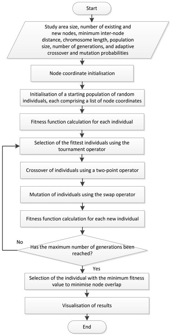
Thus, the optimal sensor node placement task is formulated as a minimisation problem, $\underset{\mathit{X} \in D^N}{\min }f\left(X\right),$ the solution to which ensures a balance between minimising redundant overlap and adhering to the minimum inter-node distance constraint for nodes with varying sensing ranges. The general structure and sequence of steps for the MGA, designed to optimise node placement, are presented in Figure 1.

Figure 1. The Proposed MGA.

The initial implementation phase involves the configuration of the input parameters shown in Figure 1.

In the subsequent stage, $\left(x,y\right)$ coordinates are randomly assigned to the network nodes. This is followed by the formation of chromosomes (individuals), each of which consists of a list of coordinates $[x_1,y_1;x_2,y_2;\cdots ,x_n,y_n]$, where each pair, $x_n,y_n$, represents the coordinates of a single node on the plane. Consequently, each chromosome within the population represents a potential node placement configuration. To determine the suitability of each individual, a fitness function is calculated to evaluate the “congestion” of the grid squares within the study plane. Accordingly, the number of nodes in each square is determined by summing the matrices for new and existing nodes.

For existing nodes, the matrix consists of 0 s and 1 s (where 1 indicates the presence of a node in a given square and 0 indicates its absence). For new nodes, the values range from 0 to $k$, where $k$ represents the number of nodes simultaneously located within a single square. If more than one node is present in a square, a value of 1 is subtracted from the total count to identify the excess. Consequently, the GA seeks solutions that minimise the number of congested squares, thereby reducing the instances of multiple nodes being placed within the same square. This ensures a more uniform distribution of nodes across the entire field, which is vital for optimal network performance. The fitness function $f\left(t_{\mathrm{n}\mathrm{e}\mathrm{t}}\right)$ can be represented as:

$$f\left(t_{\mathrm{n}\mathrm{e}\mathrm{t}}\right)={\displaystyle \sum _{i=1}^N}\mathrm{m}\mathrm{a}\mathrm{x}(0,{val}_{\mathrm{m}\mathrm{a}\mathrm{t}\mathrm{r}}\left(i\right)-1),$$

(6)

where $va{l}_{\mathrm{m}\mathrm{a}\mathrm{t}\mathrm{r}}\left(i\right)$ is the value in the matrix for each square $i$, and $N$ is the total number of squares in the study field.

Equation (6) minimises the number of redundant objects within each cell. A lower value of $f\left(t_{\mathrm{n}\mathrm{e}\mathrm{t}}\right)$ is preferable, as it indicates a more uniform distribution of objects across the squares. Once the fitness value for each individual in the initial population has been determined, they undergo modification through the following genetic operators:

• Selection stage: Tournament selection;
• Crossover stage: Two-point crossover;
• Mutation stage: Swap mutation (exchange mutation).

Subsequently, the newly formed individuals are evaluated for their suitability in solving the stated problem using (6). The termination criterion for the algorithm is the completion of a predefined number of generations, after which the individual with the lowest fitness value is selected.

Let us consider the stages of implementation of the modified GA from a programming point of view.

1. Configuration of core parameters based on the input data from Figure 1.

The application of a minimum allowable distance between nodes is intended to ensure superior area coverage and enhance network efficiency. Furthermore, this parameter prevents excessive overlapping of node sensing ranges, which could lead to redundant energy consumption and diminished network performance due to excessive data duplication and transmission conflicts. Consequently, accounting for the minimum inter-node distance is vital when planning and deploying sensor nodes to achieve optimal coverage and network functionality.

2. Development of the get_locations() function to generate a set of coordinates where sensor nodes can potentially be positioned. The objective of this stage is to define distributed points on the plane that can be utilised for subsequent optimisation via the GA.

3. Development of the get_lim_counts() function to generate random node coordinates while considering constraints for each individual node. Let the set of coordinates for potential node placement ${Loc}_{\mathrm{n}\mathrm{o}\mathrm{d}\mathrm{e}\mathrm{s}}$ be:

$${Loc}_{\mathrm{n}\mathrm{o}\mathrm{d}\mathrm{e}\mathrm{s}}=\left\{(x_i,y_i)\left|i=1,\dots ,n\right.\right\},$$

(7)

where $n$ is the number of new nodes. A subset of coordinates is randomly selected to define the initial node locations. Subsequently, the constraints for the network nodes are calculated. For each node with coordinates $(x_i,y_i)$, the following boundaries are computed:

$$x_{\mathrm{m}\mathrm{i}\mathrm{n}}=\max \left(1, x_i-\mathrm{i}\mathrm{n}\mathrm{t}\mathrm{e}{\mathrm{r}}_{\mathrm{d}\mathrm{i}\mathrm{s}\mathrm{t}\left(i\right)}\right), x_{\mathrm{m}\mathrm{a}\mathrm{x}}=\min \left(f_{\mathrm{s}\mathrm{i}\mathrm{z}\mathrm{e}}+1,x_i+\mathrm{i}\mathrm{n}\mathrm{t}\mathrm{e}{\mathrm{r}}_{\mathrm{d}\mathrm{i}\mathrm{s}\mathrm{t}\left(i\right)}+1\right),$$

(8)

$$y_{\mathrm{m}\mathrm{i}\mathrm{n}}=\max \left(1, y_i-\mathrm{i}\mathrm{n}\mathrm{t}\mathrm{e}{\mathrm{r}}_{\mathrm{d}\mathrm{i}\mathrm{s}\mathrm{t}\left(i\right)}\right), y_{\mathrm{m}\mathrm{a}\mathrm{x}}=\min \left(f_{\mathrm{s}\mathrm{i}\mathrm{z}\mathrm{e}}+1,y_i+\mathrm{i}\mathrm{n}\mathrm{t}\mathrm{e}{\mathrm{r}}_{\mathrm{d}\mathrm{i}\mathrm{s}\mathrm{t}\left(i\right)}+1\right),$$

(9)

where $i$ is the node index, $\mathrm{i}\mathrm{n}\mathrm{t}\mathrm{e}{\mathrm{r}}_{\mathrm{d}\mathrm{i}\mathrm{s}\mathrm{t}\left(i\right)}$ is the minimum inter-node distance constraint, and $f_{\mathrm{s}\mathrm{i}\mathrm{z}\mathrm{e}}$ is the dimension of the study field. These boundaries define a square area within which the coverage region of each node is situated. A grid of points falling within the node’s coverage area is then computed:

$$x_{\mathrm{r}\mathrm{a}\mathrm{n}\mathrm{g}\mathrm{e}}=\left\{x ϵ Z\left|x_{\mathrm{m}\mathrm{i}\mathrm{n}}\le x\le x_{\mathrm{m}\mathrm{a}\mathrm{x}}\right.\right\},y_{\mathrm{r}\mathrm{a}\mathrm{n}\mathrm{g}\mathrm{e}}=\left\{y ϵ Z\left|y_{\mathrm{m}\mathrm{i}\mathrm{n}}\le y\le y_{\mathrm{m}\mathrm{a}\mathrm{x}}\right.\right\}.$$

(10)

Subsequently, it is determined which points within the square also belong to the node’s circular area, taking into account the $\mathrm{i}\mathrm{n}\mathrm{t}\mathrm{e}{\mathrm{r}}_{\mathrm{d}\mathrm{i}\mathrm{s}\mathrm{t}\left(i\right)}$:

$$\mathrm{m}\mathrm{a}\mathrm{s}\mathrm{k}=\left\{\left(x,y\right)|(x_i-x{)}^2+{(y_i-y)}^2\le {{\mathrm{i}\mathrm{n}\mathrm{t}\mathrm{e}\mathrm{r}}_{\mathrm{d}\mathrm{i}\mathrm{s}\mathrm{t}\left(i\right)}}^2\right\}.$$

(11)

The coverage matrix ${\mathrm{l}\mathrm{i}\mathrm{m}}_{\mathrm{c}\mathrm{o}\mathrm{u}\mathrm{n}\mathrm{t}\mathrm{s}}$ is updated to define the frequency with which a specific point on the study plane falls within the coverage area of the nodes.

4. Initial population generation using the DEAP library, where each individual represents a potential node deployment configuration on the plane.

5. Definition of the fitness function $f\left(t_{\mathrm{n}\mathrm{e}\mathrm{t}}\right)$ to evaluate the quality of each individual; according to this function, a lower number of node overlaps indicates a superior placement configuration.

6. Configuration of genetic operators as illustrated in Figure 1.

Selection operator:

$$S=\mathrm{s}\mathrm{e}\mathrm{l}\mathrm{e}\mathrm{c}\mathrm{t}\left(P,T\right),$$

(12)

where $P$ is the current population, $T$ is the tournament size, and $S$ is the subset of individuals selected for crossover.

Crossover operator:

$$C_i=\mathrm{c}\mathrm{r}\mathrm{o}\mathrm{s}\mathrm{s}\mathrm{o}\mathrm{v}\mathrm{e}\mathrm{r}\left(P_i,P_j\right),$$

(13)

where $P_i,P_j$ are the parent individuals, and $C_i$ is the offspring (new individual) produced as a result of the crossover.

The mutation operator modifies gene values within individuals with an adaptive probability. This is achieved by selecting two random positions within an individual and subsequently swapping their values. After all GA operators have been applied, the population is updated with the new individuals:

$$P_{t+1}=S+M\left(C_i\right),$$

(14)

where $P_{t+1}$ is the updated population for the subsequent iteration of the algorithm, $S$ represents the superior individuals following selection, and $M\left(C_i\right)$ denotes the individuals after crossover and mutation.

7. Execution of the GA. The process is repeated until the predefined number of generations is reached.

8. Visualisation of the results: node placement on the plane, their sensing ranges, the minimum inter-node distance, and node “overlap” (if present).

In this study, the term “overlap” refers to the intersection of zones defined by the minimum inter-node distance radius of the sensor nodes. For each node, these zones are modelled as circles, where the centres correspond to the node coordinates and the radii correspond to the specified minimum distance value. The intersection of two or more such zones is interpreted as an overlap, which is visualised in red on the graphical representation of the node deployment. The process of determining overlap is implemented by discretizing the study area, where each metre is represented as an individual point. For each point, the algorithm determines the number of coverage zones within which it is located. If a point belongs to more than one zone, it is recorded as an instance of overlap. To represent the total amount of such overlaps across the entire study area, the overlap index $I_{\mathrm{o}\mathrm{v}\mathrm{e}\mathrm{r}\mathrm{l}\mathrm{a}\mathrm{p}}$ is used, which is defined as:

$$I_{\mathrm{o}\mathrm{v}\mathrm{e}\mathrm{r}\mathrm{l}\mathrm{a}\mathrm{p}}=\sum _{p \in P}\max \left(0,c\left(p\right)-1\right),$$

(15)

where $c\left(p\right)={\displaystyle {\sum }_{k=1}^N}{1}_{p \in C_k}$ is the coverage function at point $p$, $1$ is an indicator function, and $C_k$ is the set of points covered by the $k$-th node. If $I_{\mathrm{o}\mathrm{v}\mathrm{e}\mathrm{r}\mathrm{l}\mathrm{a}\mathrm{p}}=0,$ there is no overlap between the defined zones. Otherwise, there are points within the study area covered by more than one node, and the value of $I_{\mathrm{o}\mathrm{v}\mathrm{e}\mathrm{r}\mathrm{l}\mathrm{a}\mathrm{p}}$ represents the total number of such points.

In conclusion, the described algorithmic stages enable the optimisation of node placement within a sensor network, specifically aimed at minimising the overlap of their sensing ranges.

In the proposed method, overlap minimization is considered as one component of an integrated energy-efficient topology optimization criterion. When a specific area is simultaneously covered by multiple sensor nodes, redundant sensing and duplicate data transmissions inevitably occur. This increases the density of active nodes performing sensing and communication tasks, leading to avoidable energy expenditure in both environmental monitoring and wireless data exchange. Consequently, reducing overlap directly mitigates redundant power consumption, thereby extending the operational lifetime of the network.

To explicitly account for this relationship, we introduced the Integrated Energy Efficiency Metric (IEEM), which directly links the spatial arrangement of sensor nodes with the network energy cost:

$$F_{\mathrm{I}\mathrm{E}\mathrm{E}\mathrm{M}}=\mathrm{A}\mathrm{C}\mathrm{E}·\left(1+{\alpha ·P}_{\mathrm{o}\mathrm{v}\mathrm{e}\mathrm{r}\mathrm{l}\mathrm{a}\mathrm{p}}+{\beta ·P}_{\mathrm{m}\mathrm{i}\mathrm{s}\mathrm{s}\mathrm{i}\mathrm{n}\mathrm{g}}\right),$$

(16)

where $\mathrm{A}\mathrm{C}\mathrm{E}$ is the Average Communication Energy (average energy consumption during transmission between neighbouring nodes), $P_{\mathrm{o}\mathrm{v}\mathrm{e}\mathrm{r}\mathrm{l}\mathrm{a}\mathrm{p}}$ is the overlap fraction of node coverage areas, $P_{\mathrm{m}\mathrm{i}\mathrm{s}\mathrm{s}\mathrm{s}\mathrm{i}\mathrm{n}\mathrm{g}}$ is the fraction of unplaced nodes, and $\alpha ,\beta$ are weighting factors that determine the relative contribution of redundant sensing overlap and unplaced nodes to the overall metric value.

Increasing the value of $\alpha$ leads to a higher penalty for redundant coverage, which encourages the algorithm to form a more uniform spatial distribution of nodes and reduce excessive energy consumption. Similarly, an increase in $\beta$ raises the penalty for configurations in which some nodes cannot be deployed within the study area. In this work, the values are set to $\alpha =1$ and $\beta =1$. This choice avoids a biased optimization shift toward either solely minimizing overlap or solely maximizing node deployment. In general, the values of $\alpha$ and $\beta$ can be adapted according to the specific requirements of the WSN application.

$$\mathrm{A}\mathrm{C}\mathrm{E}={\displaystyle \frac{1}{\left|L\right|}}\sum _{\left(i,j\right) \in L}{d}_{ij}^2,$$

(17)

where $L$ is the set of all pairs of nodes that are directly connected to each other, $d_{ij}$ is the distance between nodes $i$ and $j$, $d_{ij}^2$ is the proportional energy consumption for data transmission, and $\left|L\right|$ is the number of edges.

The set $L$ is defined as the collection of all pairs of nodes $\left(i,j\right)$ between which a direct connection exists:

$$L=\left\{\left(i,j\right)\left|i\ne j, d_{ij}\ne 1000\right.\right\},$$

(18)

where $d_{ij}$ is the distance between nodes $i$ and $j$, and the value 1000 is used as a service marker indicating the absence of a direct link. Thus, nodes $i$ and $j$ are considered directly connected if a communication channel exists between them and the distance between them does not exceed the allowable communication radius. Pairs where $d_{ij}=0$ are excluded, as they represent the distance from a node to itself.

$$P_{\mathrm{o}\mathrm{v}\mathrm{e}\mathrm{r}\mathrm{l}\mathrm{a}\mathrm{p}}={\displaystyle \frac{A_{\mathrm{o}\mathrm{v}}}{A_{\mathrm{t}\mathrm{o}\mathrm{t}\mathrm{a}\mathrm{l}}}},$$

(19)

where $A_{\mathrm{o}\mathrm{v}}$ is the number of areas covered by more than one node, and $A_{total}$ is the total coverage area.

$$P_{\mathrm{m}\mathrm{i}\mathrm{s}\mathrm{s}\mathrm{i}\mathrm{n}\mathrm{g}}={\displaystyle \frac{N_{\mathrm{m}\mathrm{i}\mathrm{s}\mathrm{s}}}{N_{\mathrm{t}\mathrm{o}\mathrm{t}\mathrm{a}\mathrm{l}}}},$$

(20)

where $N_{\mathrm{m}\mathrm{i}\mathrm{s}\mathrm{s}}$ is the number of nodes that could not be placed, and $N_{\mathrm{t}\mathrm{o}\mathrm{t}\mathrm{a}\mathrm{l}}$ is the total number of nodes.

Minimizing $F_{\mathrm{I}\mathrm{E}\mathrm{E}\mathrm{M}}$ reduces routing and transmission energy costs, while the multiplicative factor $\left(1+{\alpha ·P}_{\mathrm{o}\mathrm{v}\mathrm{e}\mathrm{r}\mathrm{l}\mathrm{a}\mathrm{p}}+{\beta ·P}_{\mathrm{m}\mathrm{i}\mathrm{s}\mathrm{s}\mathrm{i}\mathrm{n}\mathrm{g}}\right)$ penalizes excessive overlap and incomplete deployment.

Thus, overlap reduction is treated as one of several contributors to energy efficiency within the IEEM objective function.

4. Analysis of the Functional Characteristics of Existing Sensor Node Placement Algorithms

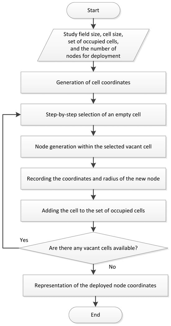
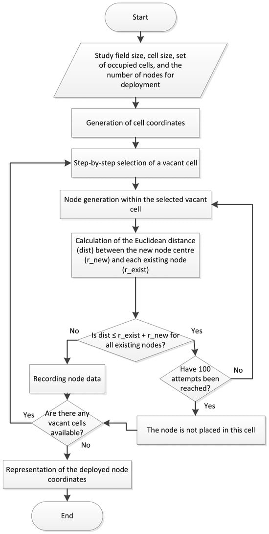
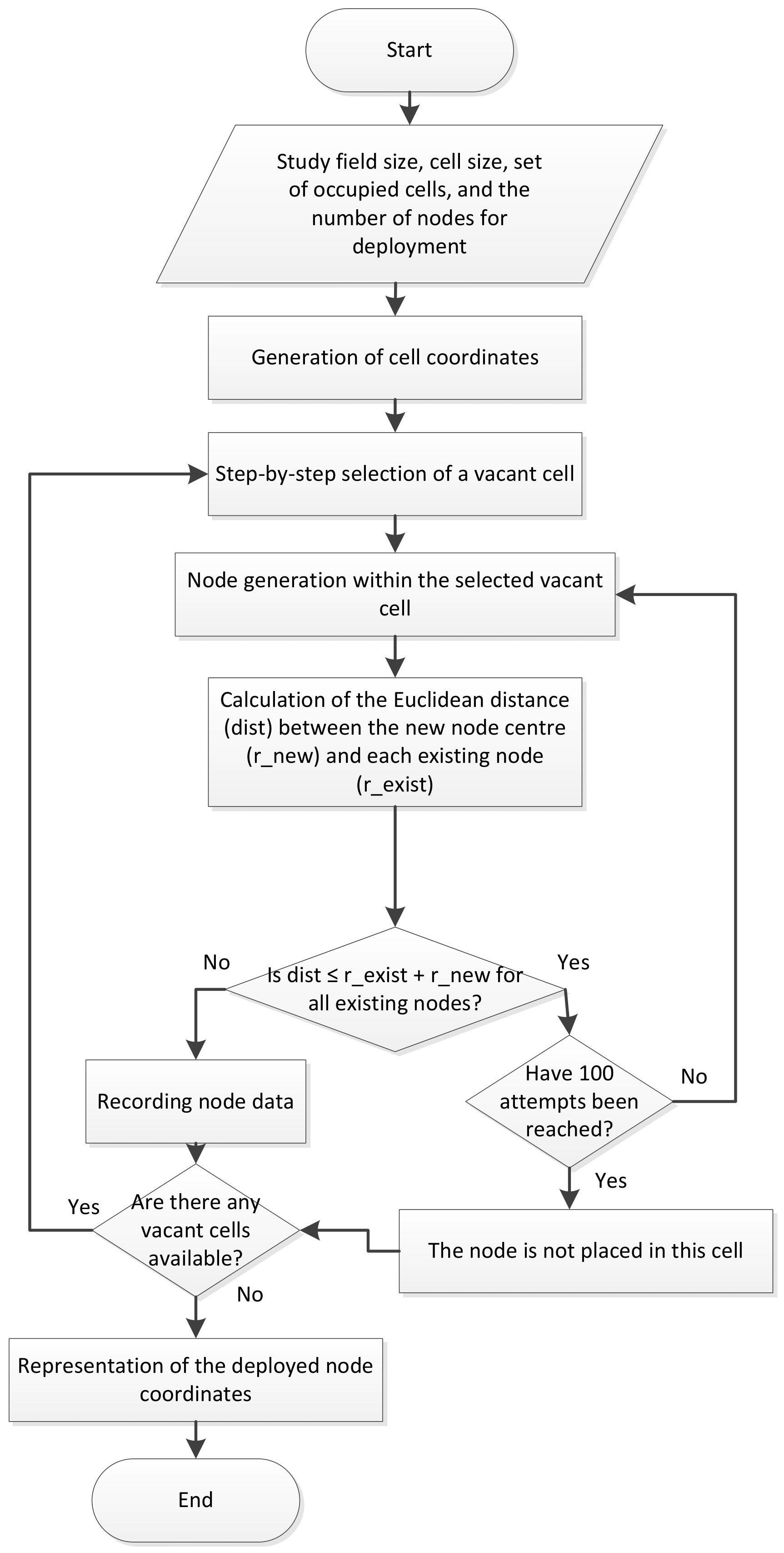
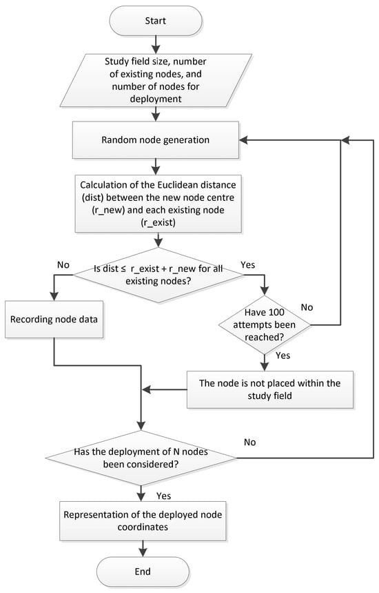
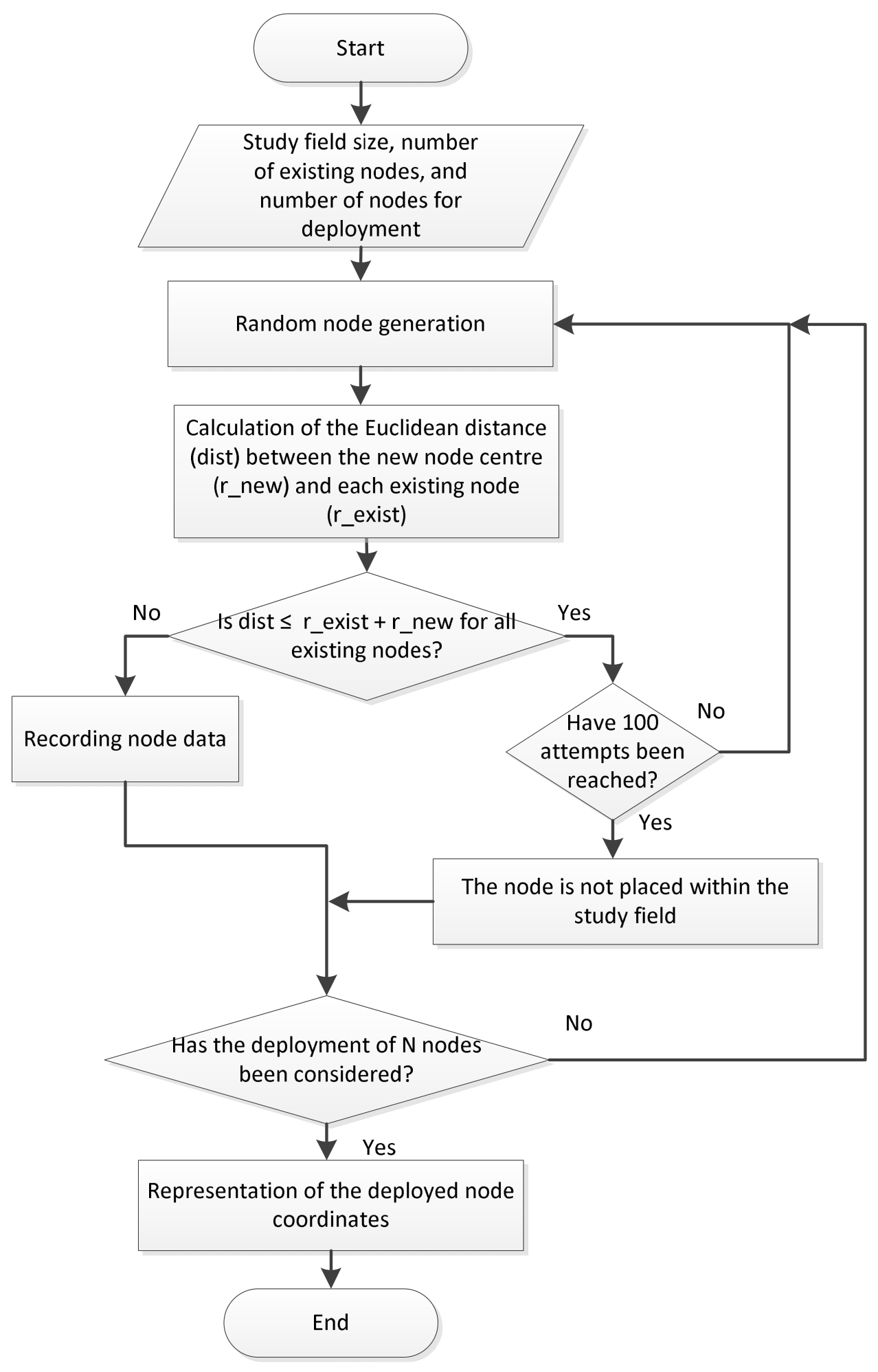
To evaluate the effectiveness of the proposed solution for WSN node deployment, a comparative analysis was conducted against representative baseline deployment strategies. These strategies reflect various approaches to WSN topology formation, namely: uniform search (mesh), greedy search, and random search [23,24,25,26]. To implement these strategies, specialized software algorithms were developed to account for the specific characteristics of WSNs; the corresponding flowcharts are presented in Figure 2, Figure 3 and Figure 4.

Figure 2. Generalised flowchart of the uniform search algorithm for WSN node placement.

Figure 3. Generalised flowchart of the greedy search algorithm for WSN node placement.

Figure 4. Generalised flowchart of the random search algorithm for WSN node placement.

The uniform search (mesh) algorithm implements regular coverage of the area by filling the discretized space; however, it does not account for constraints on the minimum inter-node distance. This is a deliberate choice, as the classical form of this approach focuses on maximizing coverage rather than optimizing the network’s spatial structure. Omitting the minimum distance check allows for the demonstration of a characteristic drawback of this approach—redundant sensing overlap.

The greedy search and random search algorithms represent a different class of strategies that apply a strict feasibility constraint: the total absence of overlap between nodes. This enables the evaluation of an opposite scenario, where overlap is completely eliminated, but at the cost of failing to deploy all nodes within the given area. This, in turn, leads to coverage loss and reduced resource efficiency.

Thus, the algorithms utilized deliberately encompass two extreme approaches to the WSN deployment problem:

-

Uniform search—full coverage with potential redundant overlap;

-

Greedy/random search—zero overlap but with incomplete node placement.

-

Consequently, the differences in the feasibility criteria of the considered algorithms provide a more comprehensive demonstration of the advantages of the proposed approach across various deployment strategies.

In the uniform search approach, the study field is partitioned into cells, within each of which a single node is randomly positioned. The objective of the algorithm is to occupy all vacant cells with a node at corresponding coordinates.

It should be noted that there is no verification of the minimum inter-node distance; while this facilitates faster deployment, it may lead to excessive node density in certain areas.

The greedy search algorithm makes sequential decisions by selecting a vacant cell and generating a node within its boundaries. The aim is to minimise overlap with other nodes by calculating the Euclidean distance between the centre of the new node and each of the existing ones.

Random search is one of the simplest approaches to implement, as it is based on the stochastic generation of node placement coordinates. Each generated node undergoes a feasibility check based on the criterion of zero overlap with existing nodes. This is determined by calculating the Euclidean distance between the centre of the potential new node and the centres of all currently deployed nodes.

5. Investigation of Stochastic Sensor Node Placement

To conduct the research, a software module was developed for the simulation and analysis of the proposed methods in WSNs, accounting for dynamically changing topologies and constrained energy and network resources. The primary objective of the module is the implementation of a GA to identify optimal spatial deployment patterns that ensure efficient coverage of a specified area. The software module was implemented using the Python programming language along with the following libraries: random for stochastic process modelling; matplotlib for data plotting and visualisation; numpy for multidimensional arrays, matrices, and mathematical operations; networkx for graph and network analysis; PyQt5 for graphical user interface development; math for mathematical functions; time for time management; DEAP for GA implementation; and sys for system and interpreter interaction.

This section presents the research results for sensor node deployment across various sensing ranges: 20, 30, and 40 m. The minimum inter-node distance constraint was adjusted accordingly. Since this constraint was modified based on its baseline value, results demonstrating the algorithm’s performance for a 25-node scenario are presented first. This approach provides a clearer visualisation of node distribution as the inter-node distance constraint varies. In Section 5.4, this case will be referred to as Case 1.

For the scenarios involving 25 nodes, the MGA was performed using the parameters specified below: a population size of 600, a maximum of 200 generations, and dynamic adjustment ranges for crossover and mutation probabilities set at [0.5; 0.8] and [0.05; 0.2], respectively [26].

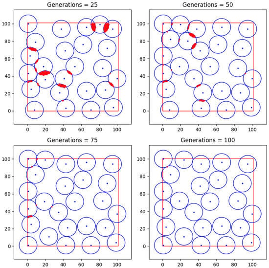
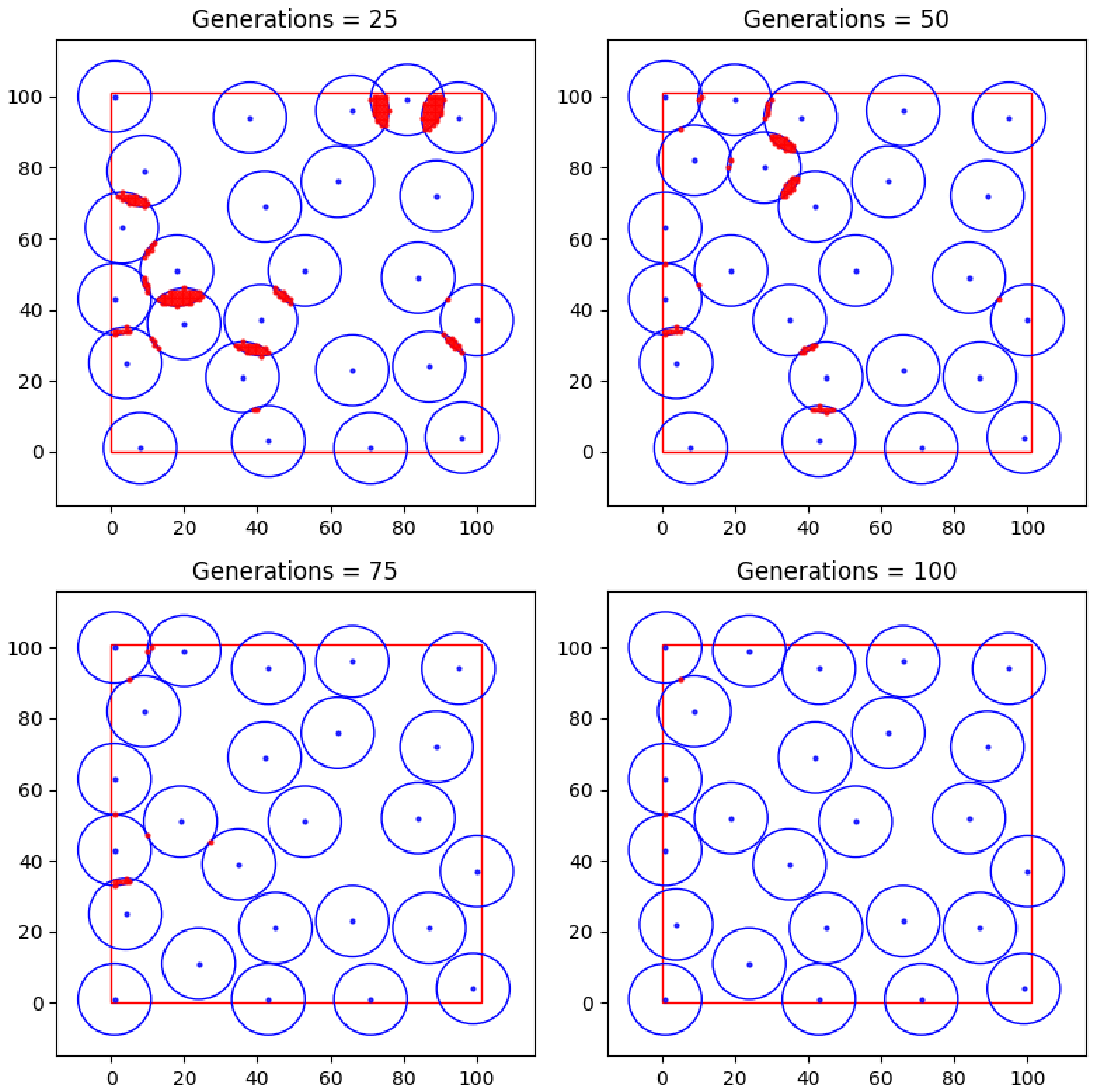
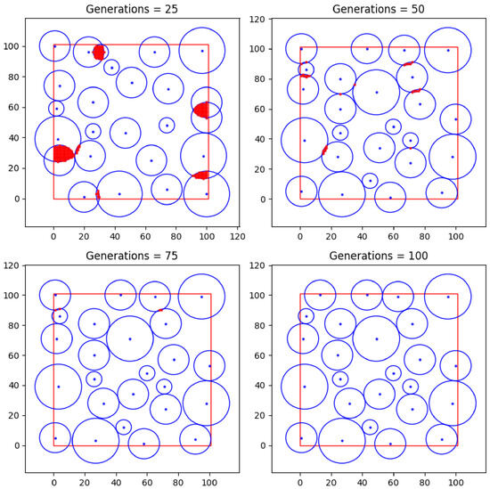
Figure 5 illustrates the step-by-step results of the proposed GA for the deployment of 25 network nodes with a minimum inter-node distance of 20 m (10 m per individual node) and a sensing range of 30 m.

Figure 5. Step-by-step performance results of the proposed algorithm for 25 network nodes.

As illustrated in Figure 5, the specified number of generations did not yield a configuration for the 25 nodes entirely free of sensing range overlaps.

The square area formed by red lines indicates the boundaries of the investigated sensor network deployment field (Figure 5). Blue circles within this area represent the sensing ranges of the sensor nodes. The central dot in each circle corresponds to the spatial position (coordinates) of the sensor node. Red intersection areas between the circles denote overlap zones of the sensing ranges of neighboring nodes, characterizing redundant coverage. These graphical notations are consistent for all similar figures presented in this work.

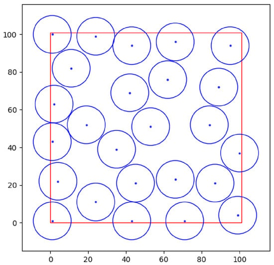
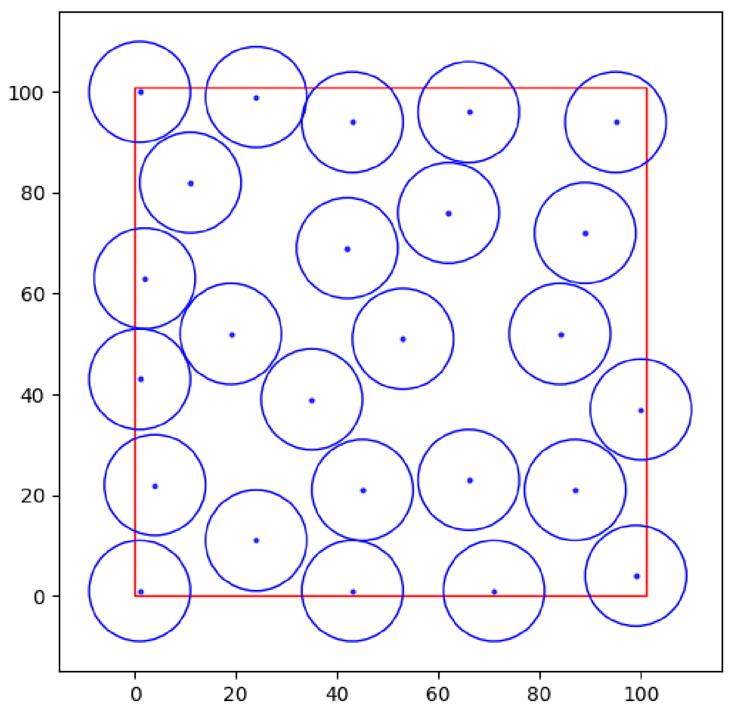
Figure 6 demonstrates the attainment of an optimal deployment for 25 nodes at $G=159$.

Figure 6. Optimal deployment of 25 nodes.

The resulting chromosome is represented as follows: [35, 39; 95, 94; 84, 52; 62, 76; 24, 11; 71, 1; 100, 37; 66, 23; 1, 1; 1, 43; 11, 82; 2, 63; 19, 52; 87, 21; 53, 51; 42, 69; 89, 72; 43, 1; 1, 100; 4, 22; 24, 99; 99, 4; 66, 96; 43, 94; 45, 21].

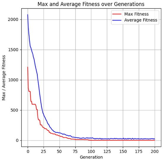
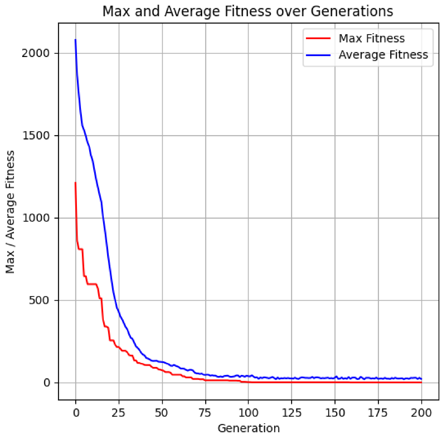
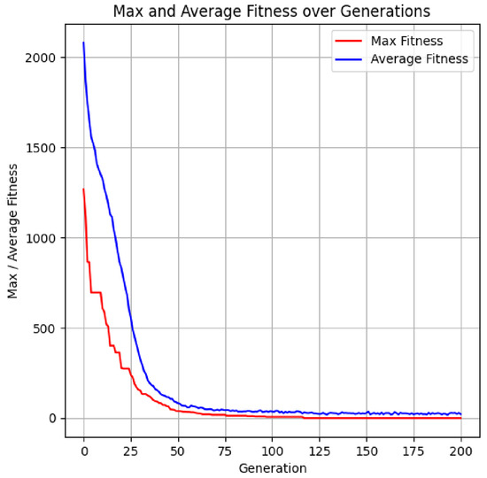
Figure 7 illustrates the impact of the number of generations on the fitness function value.

Figure 7. Influence of the number of generations on the fitness function value for 25 sensor nodes with an identical sensing range.

The illustrated graph (Figure 7) demonstrates the attainment of the optimal objective function value for the defined task.

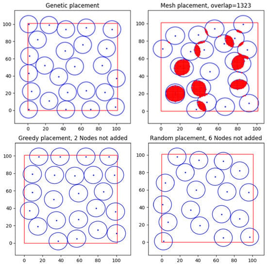
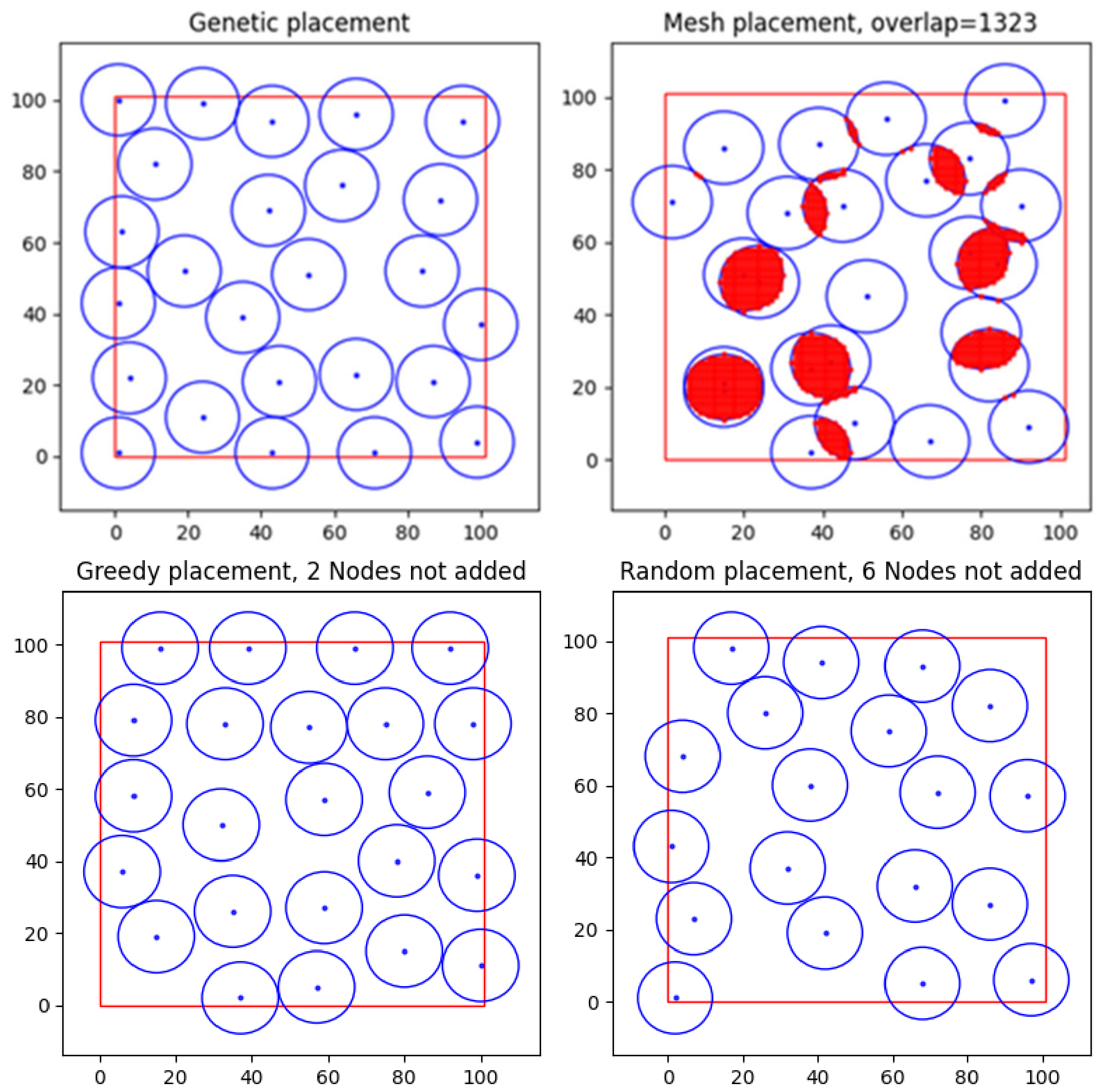
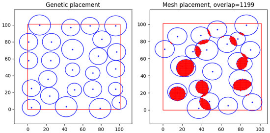
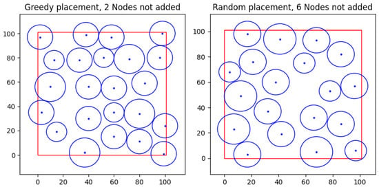
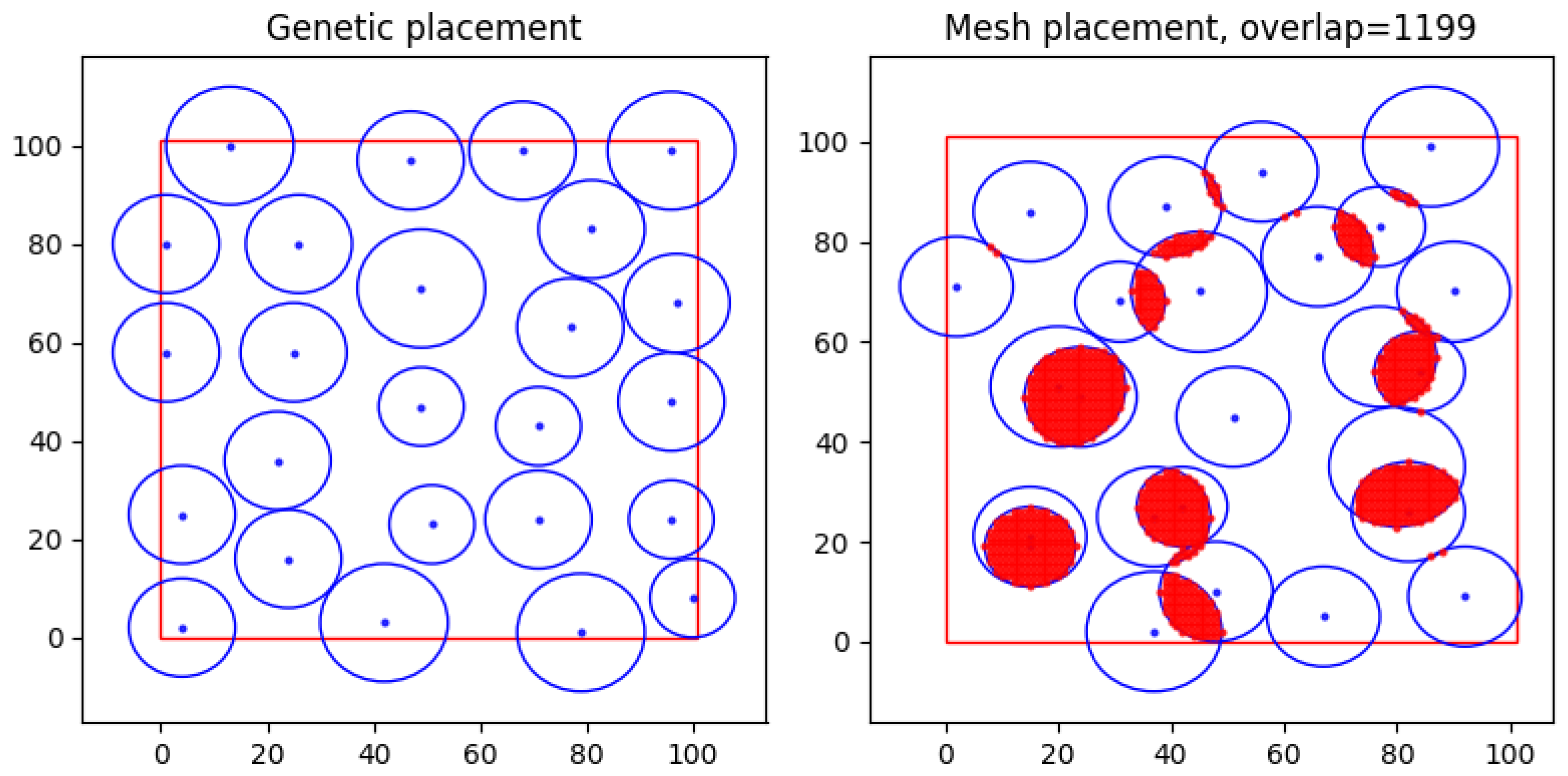
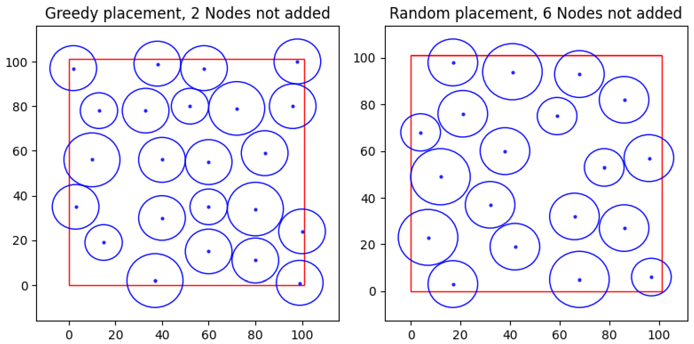
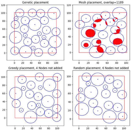
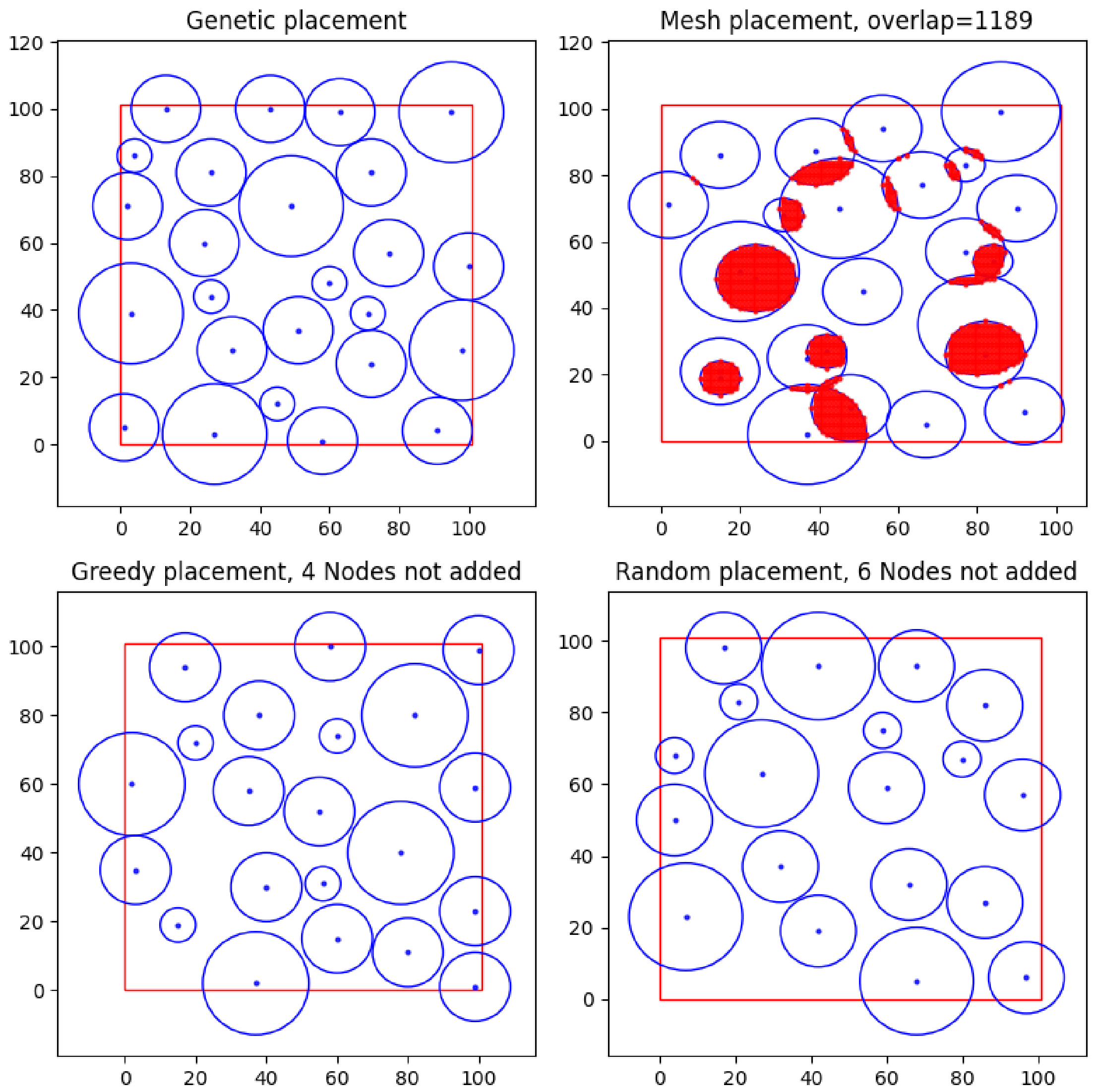
Figure 8 presents the deployment results for 25 new sensor nodes achieved using the developed Genetic algorithm, as well as the Uniform (hereinafter referred to as Mesh in the figures), Greedy, and Random algorithms.

Figure 8. Performance results of the placement algorithms for 25 new sensor nodes.

As observed in Figure 8, the developed solution successfully deployed 25 new sensor nodes within the study area under the specified conditions. The Uniform search (Mesh) is characterised by the presence of sensor node overlap zones, accounting for 13.23% of the total area. Although the Greedy and Random search methods resulted in zero overlap, they demonstrated lower efficiency during the deployment process of the 25 new nodes: the Greedy algorithm failed to place 2 nodes, while the Random search failed to place 6 nodes.

To enhance the clarity and objectivity of the comparative analysis, the simulation results are further summarized in Table 1.

Table 1. Results of the deployment of 25 sensor nodes with an identical sensing radius.

Algorithm Performance Metrics	Developed GA	Uniform Search (Mesh)	Greedy Search	Random Search
Number of deployed nodes	25	25	23	19
Node overlap area, %	-	13.23	-	-

To ensure the reproducibility of the results and to evaluate the convergence stability of the MGA, a series of experimental runs was conducted using different values for the initialization seed parameter. Varying the seed value accounts for the stochastic nature of the GA and allows for verifying the robustness of the obtained solutions against random factors affecting the initial population and the evolutionary process.

The obtained results are summarized and presented in Table 2, allowing for an assessment of the results’ variability and confirming the stability of the proposed solution. Specifically, the Seed parameter varied from 10 to 100 with a step of 10, allowing for an evaluation of the stochastic initialization’s impact on the evolutionary optimization process. The Gen parameter in the table represents the generation number at which the best fitness function value was achieved for each corresponding Seed value.

Table 2. MGA run results with different seed values.

Seed	10	20	30	40	50	60	70	80	90	100
Gen	114	200	139	159	100	144	95	119	104	148
Penalty	0	1	0	0	0	0	0	0	0	0
Overlap	0	0.0001	0	0	0	0	0	0	0	0
Missing	0	0	0	0	0	0	0	0	0	0
IEEM	522.62	537.65	541.28	507.69	531.89	548.07	576.65	535.93	539.12	526.75

The obtained results confirm the robustness of the MGA performance.

5.1. Minimum Inter-Node Distance Variation (±2 m) for 25 Sensors with Different Sensing Ranges

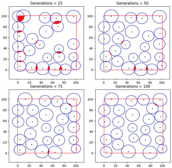
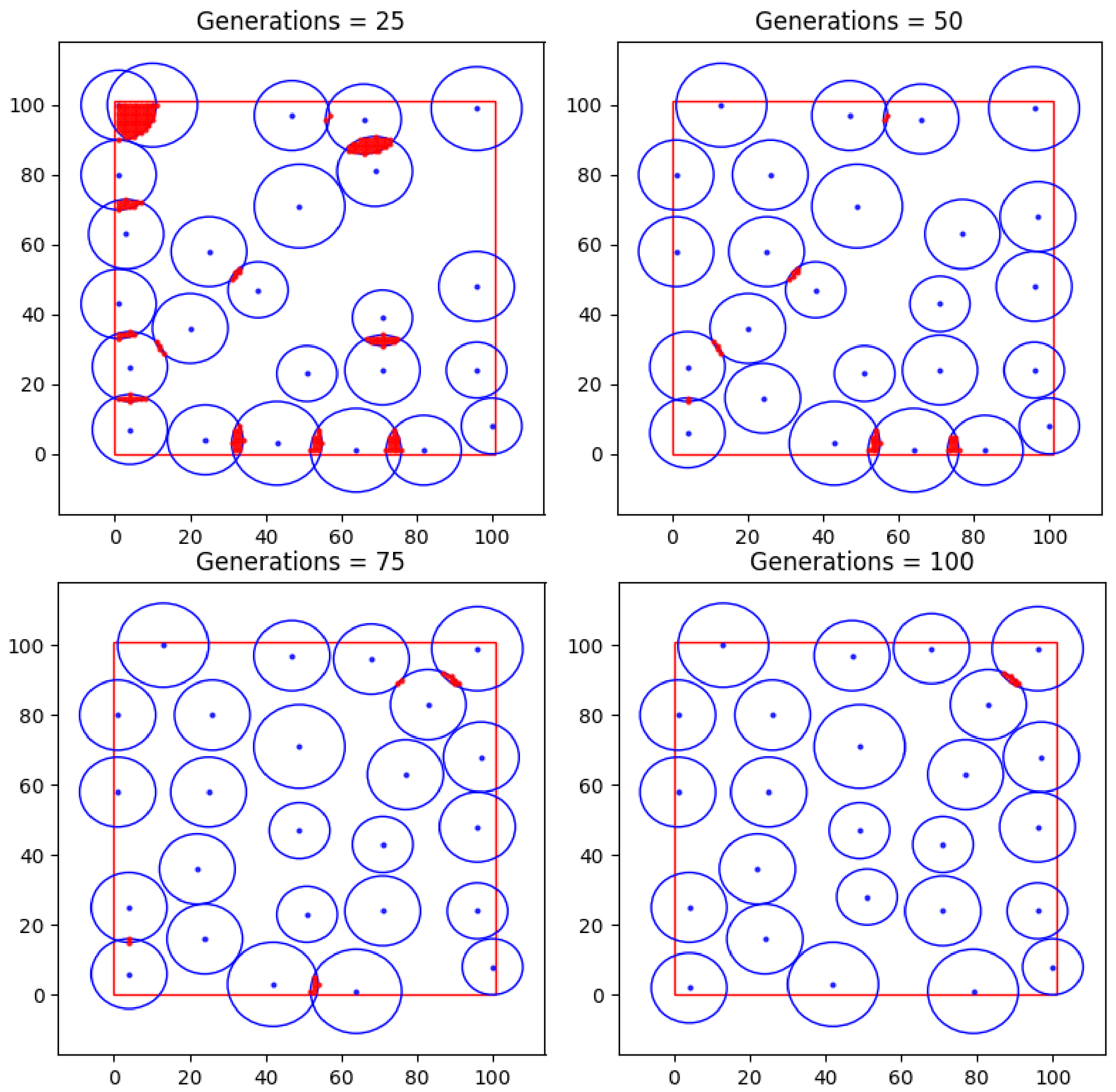
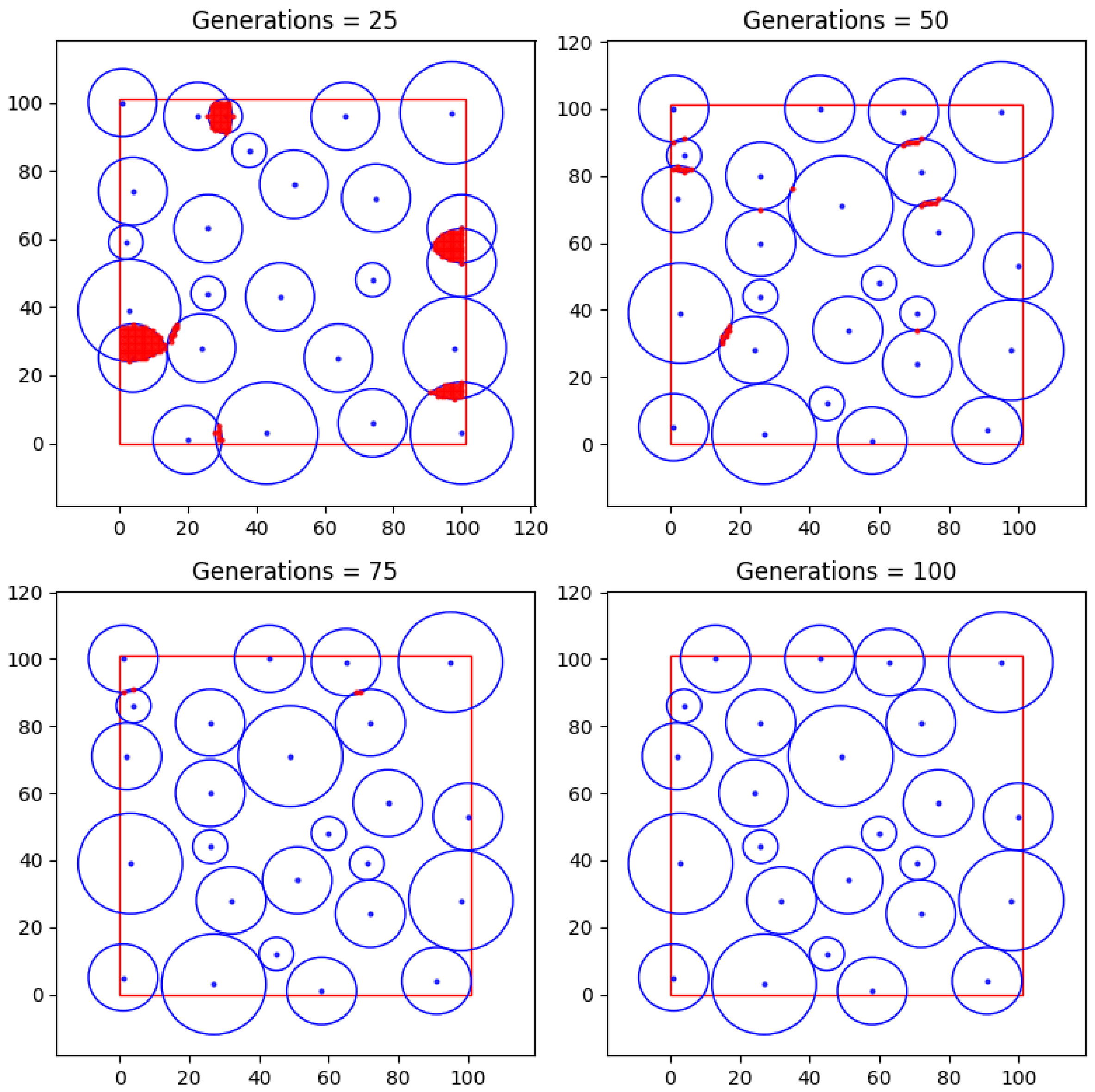
Figure 9 presents the step-by-step performance results of the proposed algorithm for the deployment of 25 network nodes, with minimum inter-node distance constraints of 8, 10, and 12 m corresponding to sensing ranges of 20, 30, and 40 m, respectively. In Section 5.4, this case will be referred to as Case 2.

Figure 9. Step-by-step performance results of the proposed algorithm for 25 network nodes with minimum inter-node distance constraints of 8, 10, and 12 m, respectively.

The presented results (Figure 9) indicate that as the number of generations increases, the algorithm’s performance is characterised by enhanced efficiency, as evidenced by the reduction in sensing range overlaps.

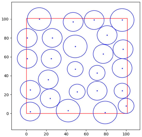
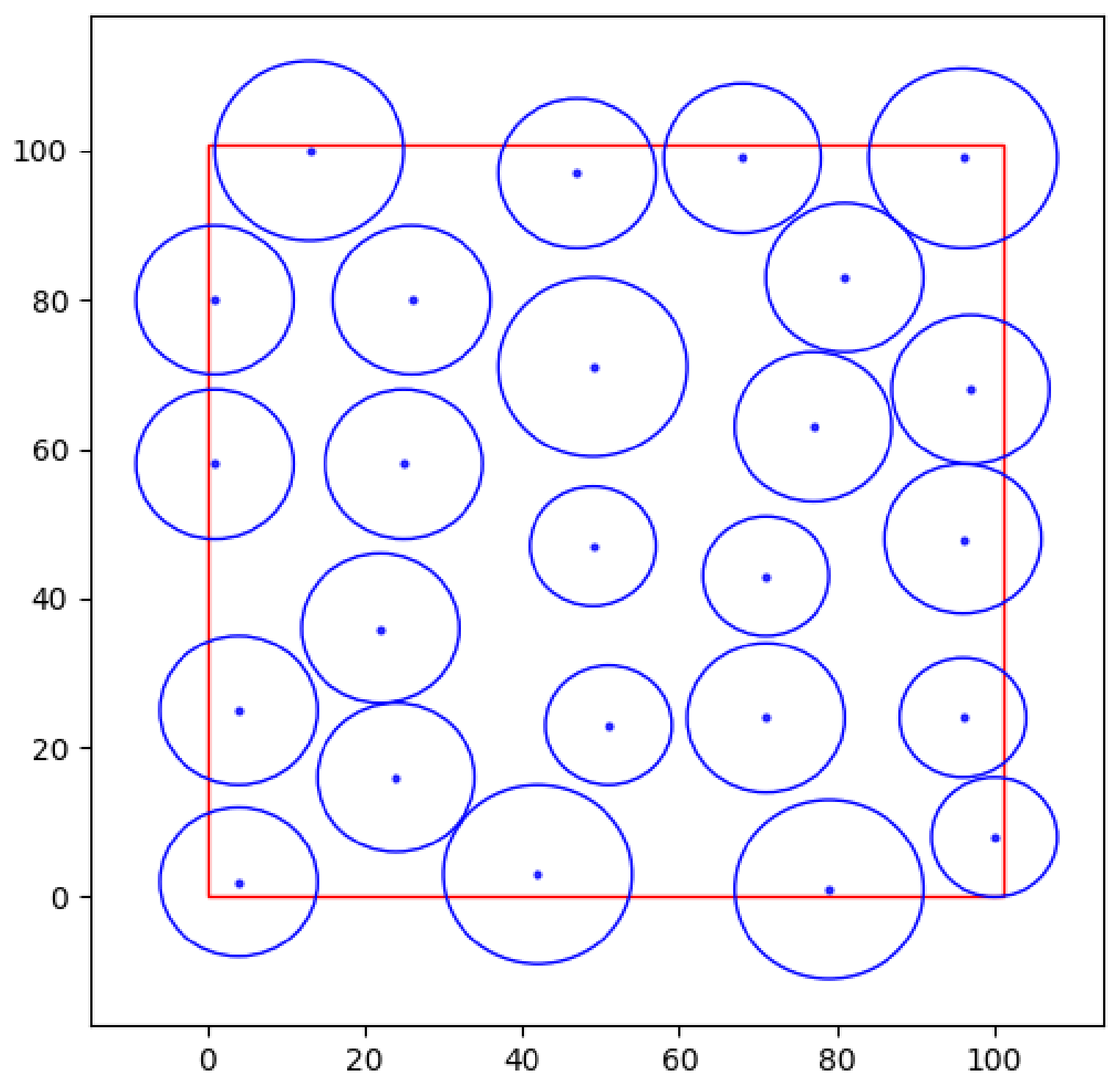
The global optimum was attained at $G=117$ (Figure 10). The resulting chromosome for this number of generations is as follows: [71, 43; 49, 71; 77, 63; 26, 80; 97, 68; 71, 24; 47, 97; 100, 8; 79, 1; 1, 80; 13, 100; 25, 58; 24, 16; 81, 83; 96, 24; 4, 2; 51, 23; 42, 3; 1, 58; 4, 25; 22, 36; 96, 48; 68, 99; 49, 47; 96, 99].

Figure 10. Optimal deployment of 25 nodes with minimum inter-node distance constraints of 8, 10, and 12 m.

To analyse the efficiency and temporal behaviour of the algorithm, Figure 11 illustrates the influence of the number of generations on the fitness function value.

Figure 11. Influence of the number of generations on the fitness function value for 25 sensor nodes with minimum inter-node distance constraints of 8, 10, and 12 m.

Figure 12 presents the deployment results for 25 new sensor nodes achieved using the developed Genetic, Mesh, Greedy, and Random algorithms, with minimum inter-node distance constraints set to 8, 10, and 12 m, respectively.

Figure 12. Performance results of the placement algorithms for 25 new sensor nodes (sensing radii of 20, 30, and 40 m) with minimum inter-node distances of 8, 10, and 12 m.

As observed in Figure 12, the developed solution successfully deployed 25 new sensor nodes within the study area under the specified conditions. The Uniform search is characterised by the presence of sensor node overlap zones, accounting for 11.99% of the total area. Although the Greedy and Random search methods resulted in zero overlap, they demonstrated lower efficiency during the deployment of the 25 new nodes: the Greedy algorithm failed to place 2 nodes, whereas the Random search failed to place 6 nodes.

5.2. Minimum Inter-Node Distance Variation (±5 m) for 25 Sensors with Different Sensing Ranges

Figure 13 illustrates the step-by-step performance results of the proposed algorithm for the deployment of 25 network nodes, with minimum inter-node distance constraints of 5, 10, and 15 m, applied to nodes with sensing ranges of 20, 30, and 40 m, respectively. In Section 5.4, this case will be referred to as Case 3.

Figure 13. Performance results of the developed placement algorithm for 25 sensor nodes with minimum inter-node distances of 5, 10, and 15 m.

As illustrated in Figure 13, within the specified number of generations, the algorithm achieved the optimal deployment of 25 nodes, accounting for the defined constraints. However, precision in reaching the global optimum is critical for this study (intermediate results are presented with a step of 25 generations).

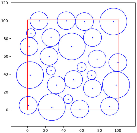
Figure 14 demonstrates its attainment at $G=90.$ The resulting chromosome is as follows: [71, 39; 49, 71; 77, 57; 26, 81; 72, 81; 72, 24; 91, 4; 26, 44; 3, 39; 100, 53; 98, 28; 43, 100; 1, 5; 2, 71; 60, 48; 51, 34; 45, 12; 27, 3; 13, 100; 63, 99; 58, 1; 32, 28; 24, 60; 4, 86; 95, 99].

Figure 14. Optimal deployment of 25 nodes with minimum inter-node distance constraints of 5, 10, and 15 m.

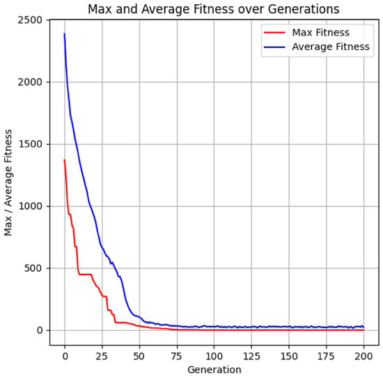
To evaluate the algorithm’s performance, the convergence rate was analysed, as shown in Figure 15.

Figure 15. Influence of the number of generations on the fitness function value for 25 sensor nodes with minimum inter-node distance constraints of 5, 10, and 15 m.

Clearly, the faster the algorithm reaches the optimum, the less time and computational resources are consumed.

The simulation results confirm the efficiency of the developed GA for the optimal deployment of sensor nodes with heterogeneous sensing ranges. These visualisations are crucial for validating the achieved convergence and objectively evaluating the quality of the identified solution, which serves as the basis for deciding whether to terminate the algorithm or proceed with further parametric optimisation.

Figure 16 presents the deployment results for 25 new sensor nodes achieved using the developed Genetic algorithm, as well as the Uniform (Mesh), Greedy, and Random search algorithms, under minimum inter-node distance constraints of 5, 10, and 15 m.

Figure 16. Performance results of the placement algorithms for 25 new sensor nodes (sensing radii of 20, 30, and 40 m) with minimum inter-node distance constraints of 5, 10, and 15 m, respectively.

As observed in Figure 16, the developed solution successfully deployed 25 new sensor nodes within the study area under the specified conditions. The Uniform search is characterised by the presence of sensor node overlap zones, accounting for 11.89% of the total area. Although the Greedy and Random search methods resulted in zero overlap, they demonstrated lower efficiency during the deployment of the 25 new nodes: the Greedy algorithm failed to place 4 nodes, whereas the Random search failed to place 6 nodes. For better clarity in comparing the performance of the considered algorithms, the obtained simulation results are presented in Table 3.

Table 3. Deployment results for 25 sensor nodes with different sensing ranges using the considered algorithms.

Deployment of 25 New Sensor Nodes with Sensing Ranges of 20, 30, and 40 m and Minimum Inter-Node Distances of 8, 10, and 12 m, Respectively
Algorithm Performance Metrics	Developed GA	Uniform Search (Mesh)	Greedy Search	Random Search
Number of deployed nodes	25	25	23	19
Node overlap area, %	-	11.99	-	-
Deployment of 25 new sensor nodes with sensing ranges of 20, 30, and 40 m and minimum inter-node distances of 5, 10, and 15 m, respectively
Algorithm performance metrics	Developed GA	Uniform Search (Mesh)	Greedy Search	Random Search
Number of deployed nodes	25	25	21	19
Node overlap area, %	-	11.89	-	-

Thus, the results of the performance evaluation for the developed algorithm in scenarios involving the deployment of 25 new sensor nodes with varying sensing radii and minimum inter-node distances demonstrate its superiority over the considered methods.

To evaluate the convergence stability of the proposed MGA, multiple trials were conducted with different initial seed values. The results obtained for 25 sensor nodes with varying sensing radii are presented in Table 4.

Table 4. MGA run results with different seed values for 25 nodes.

For 25 Sensor Nodes with Sensing Radii of 20, 30, and 40 m and Minimum Inter-Node Distances of 8, 10, and 12 m
Seed	10	20	30	40	50	60	70	80	90	100
Gen	114	70	100	117	135	192	93	118	122	72
Penalty	0	0	0	0	0	0	0	0	0	0
Overlap	0	0	0	0	0	0	0	0	0	0
Missing	0	0	0	0	0	0	0	0	0	0
IEEM	562.77	547.29	540.82	555.85	547.92	573.28	553.20	530.32	559.80	558.13
For 25 sensor nodes with sensing radii of 20, 30, and 40 m and minimum inter-node distances of 5, 10, and 15 m
Seed	10	20	30	40	50	60	70	80	90	100
Gen	160	98	117	90	94	75	95	125	80	129
Penalty	0	0	0	0	0	0	0	0	0	0
Overlap	0	0	0	0	0	0	0	0	0	0
Missing	0	0	0	0	0	0	0	0	0	0
IEEM	590.95	568.40	528.29	561.78	552.92	529.11	551.42	569.08	570.01	556.99

The data in Table 4 validate the convergence capabilities of the MGA under varying conditions.

5.3. Minimum Inter-Node Distance Variation (±2 m) for 100 Sensors with Different Sensing Ranges

To evaluate the scalability of the proposed MGA, an additional investigation was conducted involving the deployment of 100 sensor nodes. The study was performed on a square area of 200 × 200 m. The following GA parameters were used throughout the simulation: a population size of 600, a maximum of 1000 generations, and dynamic adjustment ranges for crossover and mutation probabilities set at [0.5; 0.8] and [0.05; 0.2], respectively. Three groups of sensors were considered, with sensing radii of 25, 30, and 35 m. In Section 5.4, this case will be referred to as Case 4.

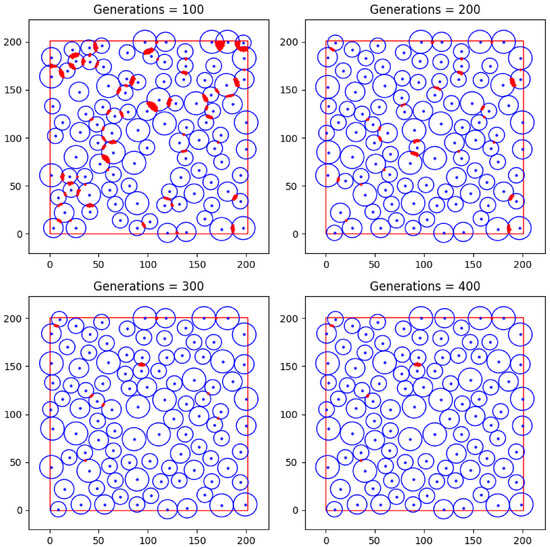
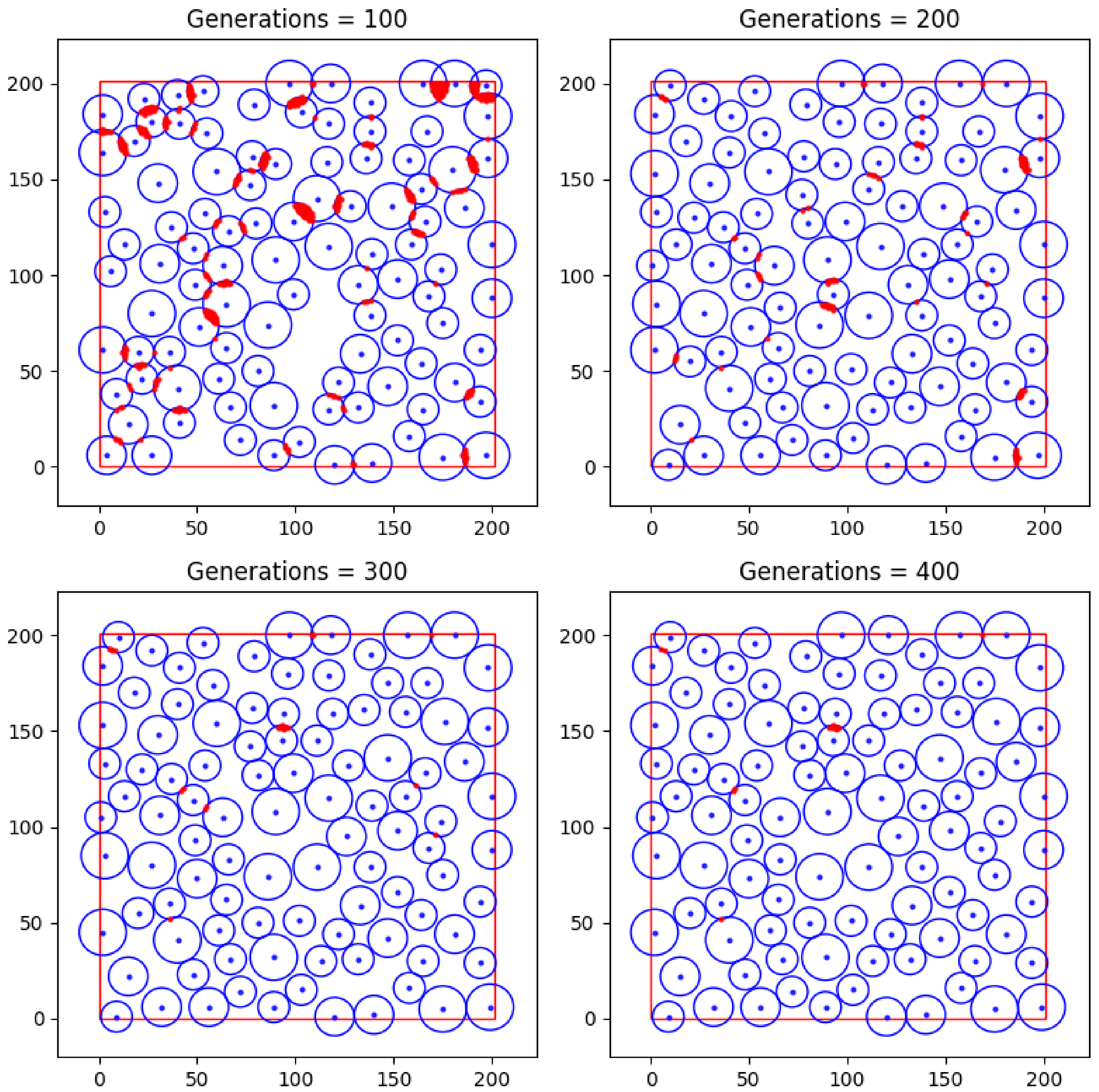
Figure 17 presents a visualisation of intermediate MGA results with an interval of 100 generations, allowing for the observation of the network topological structure formation dynamics.

Figure 17. Performance results of the developed placement algorithm for 100 new sensor nodes (sensing ranges of 25, 30, and 35 m) with minimum inter-node distance constraints of 8, 10, and 12 m at different numbers of generations.

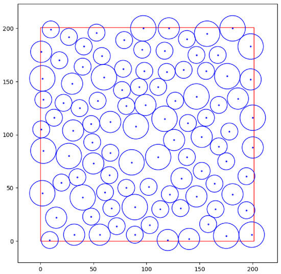
Analysis of the presented spatial configurations (Figure 17) indicates that the highest level of redundant overlap occurs at 100 generations. This is attributed to the population being in the stage of active search space exploration. However, with further iterative processing, there is a steady trend towards topological ordering: the number of sensing zone overlaps decreases monotonically. Figure 18 illustrates the attainment of the global optimum at $G=672$. The resulting chromosome is as follows: [157, 195, 121, 200, 48, 23, 168, 128, 127, 132, 198, 183, 32, 6, 54, 132, 175, 75, 164, 54, 176, 155, 126, 95, 168, 89, 138, 79, 138, 190, 27, 80, 200, 88, 93, 145, 113, 30, 119, 159, 2, 153, 99, 128, 158, 16, 77, 142, 81, 127, 200, 116, 147, 42, 41, 183, 132, 31, 20, 55, 86, 74, 66, 112, 78, 162, 152, 66, 135, 161, 199, 6, 186, 134, 49, 93, 67, 31, 147, 175, 60, 154, 140, 2, 165, 30, 79, 189, 122, 44, 40, 41, 50, 73, 22, 130, 9, 1, 13, 116, 181, 200, 120, 1, 65, 62, 27, 192, 103, 15, 97, 200, 30, 148, 111, 145, 178, 103, 18, 170, 117, 115, 152, 98, 102, 51, 40, 164, 48, 110, 175, 5, 1, 178, 72, 14, 167, 175, 156, 160, 111, 79, 15, 22, 1, 105, 35, 60, 194, 61, 90, 108, 198, 152, 37, 125, 89, 6, 53, 196, 147, 136, 56, 6, 194, 29, 3, 133, 139, 111, 3, 85, 133, 59, 10, 199, 58, 174, 98, 160, 2, 45, 31, 104, 61, 46, 81, 50, 117, 179, 89, 32, 181, 44, 156, 116, 96, 180, 66, 83].

Figure 18. Optimal deployment of 100 sensor nodes.

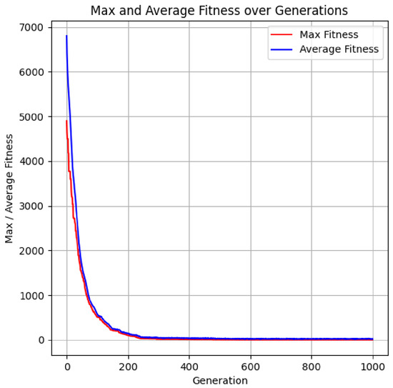
A crucial metric for evaluating the performance of the proposed method is its convergence rate. Figure 19 demonstrates the impact of the number of generations on the dynamics of the fitness function values.

Figure 19. Influence of the number of generations on the fitness function value for100 sensor nodes with minimum inter-node distance constraints of 8, 10, and 12 m.

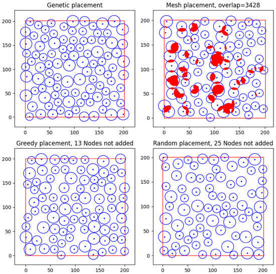
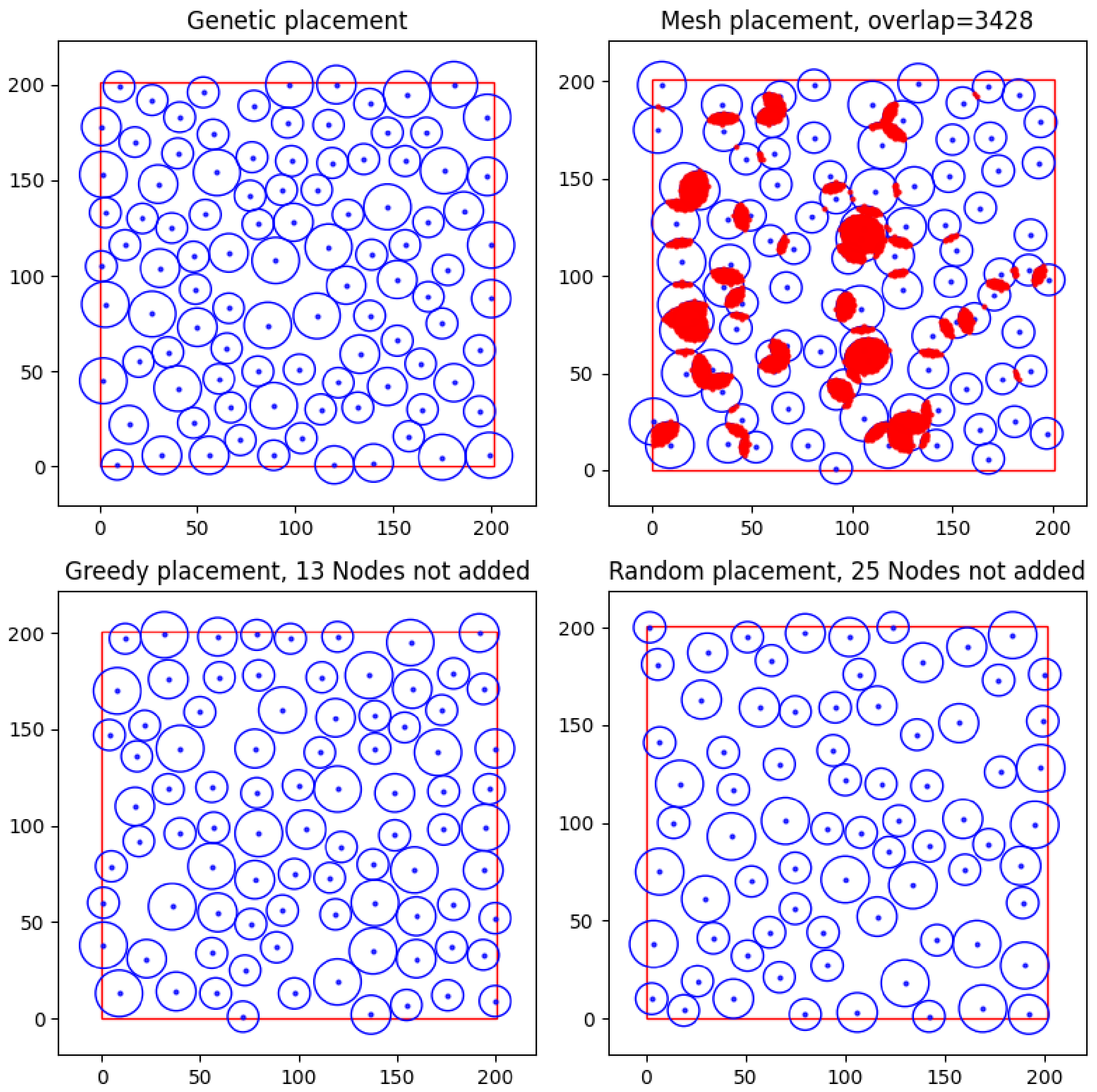
Figure 20 presents the deployment results for 100 new sensor nodes achieved using the developed GA, as well as the Uniform (Mesh), Greedy, and Random search algorithms, under minimum inter-node distance constraints of 8, 10, and 12 m.

Figure 20. Performance results of the placement algorithms for 100 new sensor nodes (sensing ranges of 25, 30, and 35 m) with minimum inter-node distances of 8, 10, and 12 m.

Analysis of the obtained results (Figure 20) confirms the high scalability and efficiency of the developed MGA method. The algorithm ensures the full integration of a specified number of sensor nodes within the study area, while adhering to the defined constraints on minimum inter-node distance and sensing ranges. This demonstrates the algorithm’s capability to form a topologically consistent network structure, even under conditions of high deployment density.

Comparative analysis shows that the Uniform Search (Mesh) algorithm, despite ensuring full node deployment, is characterised by a significant level of redundant sensing overlap, amounting to 34.28% of the total monitoring area. This result indicates an inefficient use of spatial and energy resources, as a substantial portion of the sensor nodes duplicate each other’s functions.

In turn, the Greedy Search and Random Search algorithms demonstrate an opposite trend: the absence of sensing overlap (0%) is achieved at the expense of incomplete node deployment. Specifically, the Greedy algorithm fails to integrate 13 nodes, while the Random Search fails to place 25 nodes. This indicates their limited ability to simultaneously utilise the available area effectively and adhere to the specified spatial constraints.

To summarise and provide a clearer comparison of the performance of the considered algorithms, the corresponding simulation results are presented in Table 5.

Table 5. Deployment of 100 new sensor nodes with sensing ranges of 25, 30, and 35 m and minimum inter-node distances of 8, 10, and 12 m, respectively.

Algorithm Performance Metrics	Developed GA	Uniform Search (Mesh)	Greedy Search	Random Search
Number of deployed nodes	100	100	87	75
Node overlap area, %	–	8.57	–	–

The robustness of the MGA’s convergence was assessed by performing a series of independent runs, each initialized with a distinct random seed. Table 6 summarizes the findings for a 100-node network configuration characterized by varying sensing radii.

Table 6. MGA run results with different seed values for 100 nodes.

Seed	10	20	30	40	50	60	70	80	90	100
Gen	1000	1000	1000	1000	748	1000	1000	672	1000	1000
Penalty	4	3	2	4	0	7	6	0	4	4
Overlap	0.0001	0.000075	0.00005	0.0001	0	0.000175	0.00015	0	0.0001	0.0001
Missing	0	0	0	0	0	0	0	0	0	0
IEEM	496.30	502.77	489.22	493.98	503.04	500.02	483.47	479.85	495.35	492.64

Thus, the results demonstrate that the proposed MGA achieves a balance between the completeness of node deployment and the minimisation of sensing overlap, ensuring more efficient use of network resources. This confirms the suitability of the algorithm for WSN deployment tasks, particularly in resource-constrained environments where uniform spatial coverage is required.

5.4. Energy Efficiency Assessment of Network Topologies

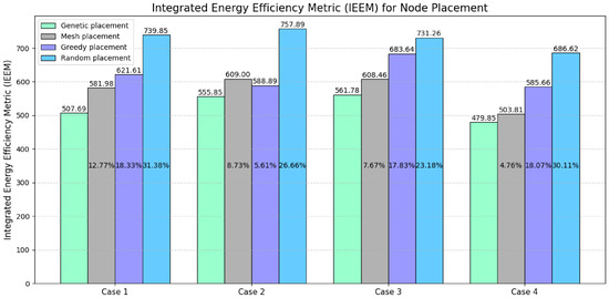
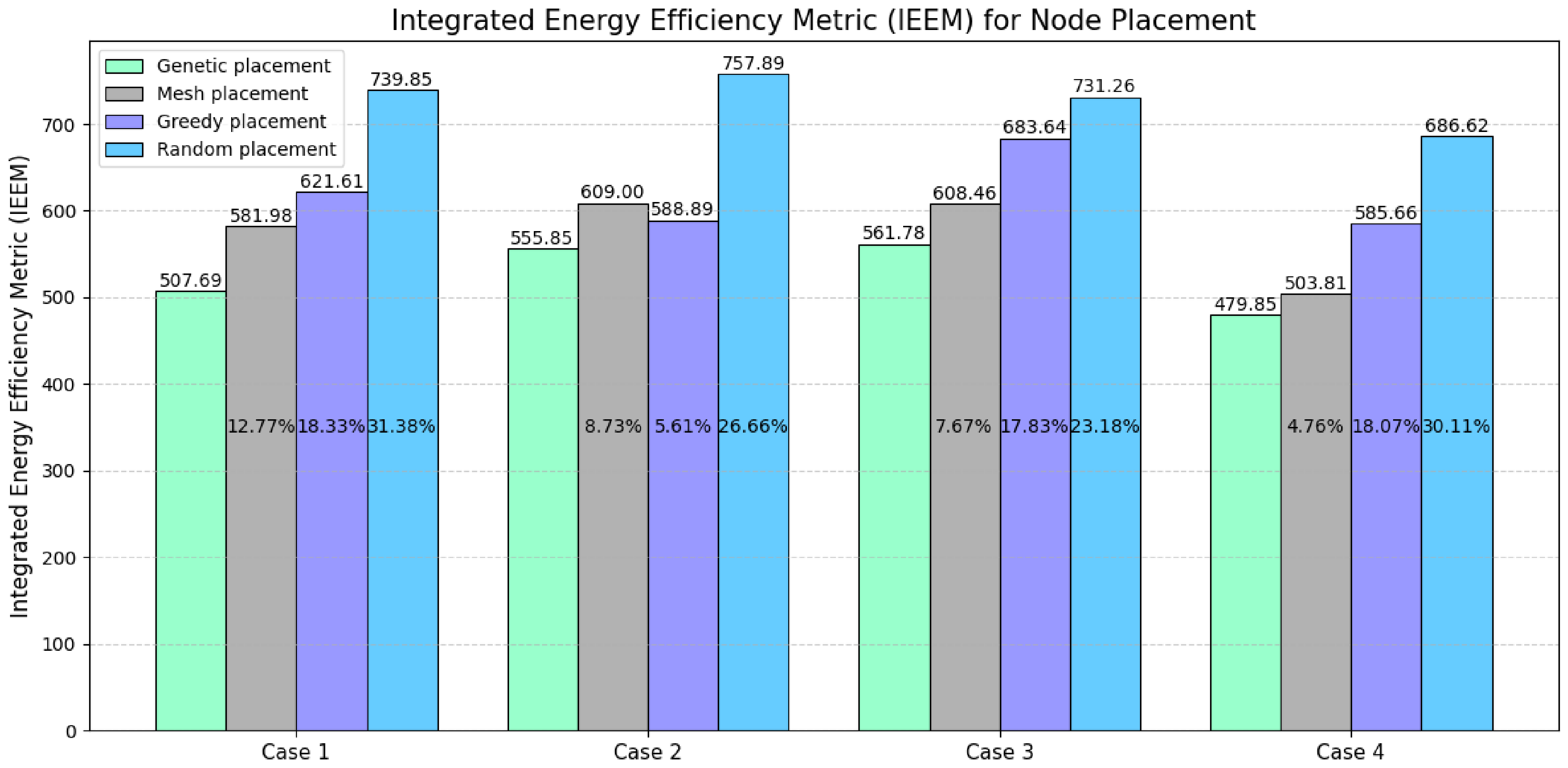
The effectiveness of the proposed MGA was evaluated by comparing it against the aforementioned methods across three WSN deployment scenarios. For each scenario, the integral energy efficiency metric was calculated, where lower values indicate higher energy efficiency of the network topology. The simulation results are presented in Figure 21.

Figure 21. Energy efficiency of topologies generated by different algorithms based on the IEEM.

As shown in Figure 21, the proposed GA outperforms all other examined methods, consistently achieving the lowest possible values of the integral energy efficiency metric across all scenarios. In contrast, the Mesh, Greedy, and Random node placement algorithms demonstrated significant energy losses. Specifically, performance metrics for these algorithms ranged from 12.77% to 31.38% in the first case, from 5.61% to 26.66% in the second, from 7.67% to 23.18% in the third, and from 4.76% to 30.11% in the fourth.

Consequently, in all studied cases, the proposed GA demonstrates a near-total minimization of redundant coverage and ensures the successful deployment of the planned number of sensor nodes. This performance significantly surpasses that of the other algorithms, which fail to avoid energy losses stemming from either spatial redundancy or incomplete coverage of the target area.

Thus, the results confirm that the proposed MGA is well-suited for topology optimization in WSN and can be effectively applied under conditions of high node density and strict spatial constraints.

6. Discussion and Conclusions

This work addresses the problem of optimal sensor node deployment without overlapping sensing ranges, utilizing a GA to enhance network efficiency. The authors have developed an MGA that evaluates the deployment area through node density metrics and a penalty-based fitness function to identify balanced configurations. This approach optimizes coverage within the study area while accounting for heterogeneous sensing radii and minimum inter-node distance constraints.

The experimental results confirm the superior efficiency of the proposed approach in WSN deployment compared to existing methods. An analysis of Greedy and Random search strategies revealed their fundamental inability to ensure full network deployment under the specified conditions.

In the investigated scenarios involving 25 sensor nodes, the Greedy algorithm failed to deploy two nodes in Scenarios 1 and 2, and four nodes in Scenario 3, whereas the Random Search algorithm failed to deploy six nodes in each scenario. From an optimization theory perspective, the Greedy search’s failure stems from its tendency to get trapped in local optima by making locally optimal decisions early on, leading to a spatial deficit for subsequent nodes. Random search, conversely, demonstrates poor performance in solution spaces with stringent constraints. The MGA, through its crossover and mutation operators, successfully overcomes local optima, ensuring global convergence and placing 100% (25 out of 25) of the nodes despite varying radii and distances.

A key finding is the comparison with the Uniform (Mesh) search. Although the Uniform search also placed all 25 nodes in both scenarios, it generated redundant overlaps of 11.99% and 11.89% of the area. The proposed GA achieved a zero-overlap (0%) metric.

To evaluate the performance of the MGA as the problem dimensionality increases, a scenario involving the deployment of 100 sensor nodes was examined, allowing for an analysis of the method’s stability under increased network density. Simulation results demonstrate that the MGA achieved full placement of all nodes, whereas Greedy Search and Random Search only managed to place 87 and 75 nodes, respectively. Although Uniform Search (Mesh) also ensured full placement, it resulted in significant redundant coverage, accounting for 8.57% of the monitored area. Thus, the proposed MGA simultaneously satisfied two critical requirements: complete node placement and the absence of substantial coverage duplication.

Analysis of repeated algorithm runs with varying initial seeds showed that the MGA is characterized by high robustness and reproducibility of results. In all ten independent trials for the 100-node scenario, full node placement was achieved, with overlap values remaining virtually zero and never exceeding 0.000175.

In this study, an Integrated Energy Efficiency Metric (IEEM) is developed, which formalizes the analytical relationship between the spatial configuration of nodes and the total energy consumption of the network.

The IEEM combines the Average Communication Energy (ACE) with penalty terms accounting for redundant coverage and incomplete node deployment. This formulation enables simultaneous control of communication cost, sensing redundancy, and deployment feasibility. The inclusion of weighting factors provides flexibility for adapting the optimization process to application-specific requirements.

Simulation results across multiple deployment scenarios demonstrate that the proposed modified genetic algorithm (MGA) consistently achieves the lowest IEEM values compared to Mesh, Greedy, and Random placement strategies. The observed improvements range from 4.76% to 31.38%, depending on the scenario, indicating substantial reductions in energy losses. These gains are primarily attributed to effective suppression of coverage overlap and complete utilization of available sensor nodes.

Consequently, the study confirms that the proposed MGA is a scalable and robust method for the node placement problem in wireless sensor networks. The algorithm maintains high solution quality even as the node count increases, ensuring full coverage, minimal overlap, and consistent results regardless of the initial seed value.

Future development of this approach will focus on extending the functional capabilities of the MGA to three-dimensional (3D) spaces, enabling optimized WSN deployment in complex terrains and multi-storey architectural structures, and next-generation 5G communication environments [27].

References

- Muthukkumar, M.S.; Arun Kumar, C.M. Enhancing Sensor Node Energy Efficiency in Wireless Sensor Networks through an Adaptable Power Allocation Framework. Int. J. Wirel. Microw. Technol. 2025, 15, 1–9. [Google Scholar] [CrossRef] [Scilit]
- Yadava, R.R.; Ranvijay, R. Green Optimization with Load balancing in Wireless Sensor Network using Elephant Herding Optimization. Int. J. Comput. Netw. Inf. Secur. 2024, 16, 120–129. [Google Scholar] [CrossRef] [Scilit]
- Singh, S.; Chand, S.; Kumar, B. Performance Evaluation of Distributed Protocols Using Different Levels of Heterogeneity Models in Wireless Sensor Networks. Int. J. Comput. Netw. Inf. Secur. 2015, 7, 38–45. [Google Scholar] [CrossRef] [Scilit]
- Kapoor, M.; Pathak, B.K.; Kuamr, R. Enhanced NSGA-II Algorithm for Solving Real-world Multi-objective Optimization Problems. Int. J. Intell. Syst. Appl. 2025, 17, 105–117. [Google Scholar] [CrossRef] [Scilit]
- Pyrih, Y.; Klymash, M.; Pyrih, Y. Genetic Approach for Balanced Placement of Wireless Sensor Network Nodes. In Proceedings of the 2025 IEEE 13th International Conference on Intelligent Data Acquisition and Advanced Computing Systems: Technology and Applications (IDAACS), Gliwice, Poland, 4–6 September 2025; pp. 1–5. [Google Scholar] [CrossRef] [Scilit]
- Gupta, S.K.; Kuila, P.; Jana, P.K. Genetic Algorithm for k-Connected Relay Node Placement in Wireless Sensor Networks. In Proceedings of the Second International Conference on Computer and Communication Technologies; Advances in Intelligent Systems and Computing; Springer: Singapore, 2016; Volume 379, pp. 1–12. [Google Scholar]
- Fischer, C.; Berndt, M.; Krummacker, D.; Zemitis, J.; Fraunholz, D.; Schotten, H.D. Industrial Network Topology Generation with Genetic Algorithms. In Proceedings of the 2020 International Young Engineers Forum (YEF-ECE), Costa da Caparica, Portugal, 2–3 July 2020; pp. 25–32. [Google Scholar] [CrossRef] [Scilit]
- Abdulelah Abbas, S.; Farzinvash, L.; Zolfy, M. A Two-Phase Genetic Algorithm Approach for Sleep Scheduling, Routing, and Clustering in Heterogeneous Wireless Sensor Networks. Network 2025, 5, 50. [Google Scholar] [CrossRef] [Scilit]
- Wang, Z.-J.; Zhan, Z.-H.; Zhang, J. Solving the Energy Efficient Coverage Problem in Wireless Sensor Networks: A Distributed Genetic Algorithm Approach with Hierarchical Fitness Evaluation. Energies 2018, 11, 3526. [Google Scholar] [CrossRef] [Scilit]
- Jia, R.; Zhang, H. Wireless Sensor Network (WSN) Model Targeting Energy Efficient Wireless Sensor Networks Node Coverage. IEEE Access 2024, 12, 27596–27610. [Google Scholar] [CrossRef] [Scilit]
- Xu, S.; Zhong, C. Optimization of Relay Node Deployment in Wireless Sensor Communication Networks Based on IGA-RNDP Algorithm. IEEE Access 2025, 13, 139506–139523. [Google Scholar] [CrossRef] [Scilit]
- Bharathi, P.S.; Pavithra, R. Modified Bron–Kerbosch-Based Sensor Deployment Algorithm for Target Coverage in Wireless Sensor Networks. IEEE Access 2025, 13, 95692–95705. [Google Scholar] [CrossRef] [Scilit]
- Karimi-Bidhendi, S.; Jafarkhani, H. Outage-Aware Deployment in Heterogeneous Rayleigh Fading Wireless Sensor Networks. IEEE Trans. Commun. 2024, 72, 1146–1161. [Google Scholar] [CrossRef] [Scilit]
- Neggaz, N.; Seyyedabbasi, A.; Hussien, A.G.; Rahim, M.; Beşkirli, M. Optimal Nodes Localization in Wireless Sensor Networks Using Nutcracker Optimizer Algorithms: Istanbul Area. IEEE Access 2024, 12, 67986–68002. [Google Scholar] [CrossRef] [Scilit]
- Afizudeen, S.; Pavithra, R. Grundy Number-Based Optimal Sensor Placement in 3D Wireless Sensor Network. IEEE Access 2024, 12, 148502–148515. [Google Scholar] [CrossRef] [Scilit]
- Kashyap, A.; Sahu, K.; Verma, L.; Jaiswal, K. DMPA–GWO++: A Dynamic Multi-Pack Adaptive Grey Wolf Optimizer for IoT Sensor Network Recovery in Smart Farms. Eng. Proc. 2025, 110, 6. [Google Scholar] [CrossRef] [Scilit]
- Wang, B.; Yan, Y.; Zhu, L.; Yin, S.; Yang, Y. MESDO: A Multi-Strategy Supply Demand Optimization for Global Optimization and Deployment of Wireless Sensor Network. Mathematics 2025, 13, 3727. [Google Scholar] [CrossRef] [Scilit]
- Yang, X.; Zhang, M. CQLHBA: Node Coverage Optimization Using Chaotic Quantum-Inspired Leader Honey Badger Algorithm. Biomimetics 2025, 10, 850. [Google Scholar] [CrossRef] [Scilit] [PubMed]
- Birtane Akar, S.; Korkmaz, H.; Sahingoz, O.K. Efficient Deployment of Wireless Sensor Nodes with Evolutionary Approaches. In Proceedings of the 2022 International Congress on Human-Computer Interaction, Optimization and Robotic Applications (HORA), Ankara, Turkey, 19–21 May 2022; pp. 1–7. [Google Scholar] [CrossRef] [Scilit]
- Mishra, R.; Jha, S.K.; Kshetri, N.; Bhusal, B.; Rahman, M.M.; Rana, M.M.; Eli, A.A.; Islam, K.A.; Pokharel, B.P. NodeWSNsec: A Hybrid Metaheuristic Approach for Reliable Security and Node Deployment in Wireless Sensor Networks. Int. J. Adv. Comput. Sci. Appl. 2025, 16, 814. [Google Scholar] [CrossRef] [Scilit]
- Pyrih, Y.; Masiuk, A.; Pyrih, Y.; Urikova, O. Investigation of a Genetic Algorithm for Solving the Travelling Salesman Problem. In Digital Ecosystems: Interconnecting Advanced Networks with AI Applications; Luntovskyy, A., Klymash, M., Melnyk, I., Beshley, M., Schill, A., Eds.; Springer: Cham, Switzerland, 2024; Volume 1198, pp. 410–427. [Google Scholar] [CrossRef] [Scilit]
- Bečejac, V.; Šošić, D.; Savić, A. Graph-Guided Genetic Algorithm for Optimal PMU Placement Ensuring Topological and Numerical Observability. Energies 2026, 19, 927. [Google Scholar] [CrossRef] [Scilit]
- Kukade, M.S.; Hande, K.N. Analysis of Uniform Distribution of Storage Nodes in Wireless Sensor Network. Int. J. Comput. Sci. Eng. 2014, 2, 43–47. [Google Scholar]
- Tiwari, J.K.; Bhardwaj, N. Improved coverage of node placement using greedy approach on scent marking of territorial predator. Int. J. Adv. Eng. Res. Dev. 2018, 5, 264–270. [Google Scholar]
- Anand, N.; Ranjan, R.; Rai, B.S.; Varma, S. A novel computational geometry-based node deployment scheme in 3D wireless sensor network. Int. J. Sens. Netw. 2017, 25, 135–145. [Google Scholar] [CrossRef] [Scilit]
- Pyrih, Y.; Klymash, M.; Pyrih, Y.; Hordiichuk-Bublivska, O. Genetic Algorithm for Routing in Sensor Networks with Dynamic Topology. In Networks and Sustainability; Luntovskyy, A., Klymash, M., Melnyk, I., Beshley, M., Gütter, D., Eds.; Springer: Cham, Switzerland, 2025; Volume 1473, pp. 410–427. [Google Scholar] [CrossRef] [Scilit]
- Przystupa, K.; Beshley, M. IBN and Service Management for 5G and Beyond; Routledge: London, UK, 2025. [Google Scholar]
Disclaimer/Publisher’s Note: The statements, opinions and data contained in all publications are solely those of the individual author(s) and contributor(s) and not of MDPI and/or the editor(s). MDPI and/or the editor(s) disclaim responsibility for any injury to people or property resulting from any ideas, methods, instructions or products referred to in the content. |
© 2026 by the authors. Licensee MDPI, Basel, Switzerland. This article is an open access article distributed under the terms and conditions of the Creative Commons Attribution (CC BY) license.