


Abstract
Ocular diseases can range in severity, with some being more serious than others. As a matter of fact, there are several common and severe eye diseases, for instance, glaucoma, i.e., a group of eye conditions that damage the optic nerve, often associated with elevated intraocular pressure. Effective management and prevention strategies require a multifaceted approach, involving healthcare providers, public health officials and community education. Regular screenings and early interventions are crucial in reducing the impact of eye diseases on individuals and populations. In this paper, we propose a method aimed to detect the presence of ocular disease from the automatic analysis of eye fundus photographs. We consider deep learning; in detail, we adopt several convolutional neural networks aimed to train several models to be able to discriminate between different eye diseases. Furthermore, to boost the application of deep learning in real-world everyday medical practice, we adopt a method to understand which areas of the images are of interest from the model’s point of view; this allows us to detect disease by providing in this way disease localization by explainability. In the experimental analysis, we provide a set of four different experiments: in the first one, we propose a model to discern between age-related macular degenerations and normal fundus (obtaining an accuracy of 0.91); in the second one, the model is able to discriminate between cataract and normal fundus (obtaining an accuracy of 0.92); the third experiment is related to a model aimed to discriminate between glaucoma and normal ocular fundus (obtaining an accuracy of 0.88); and the last experiment is related to a model aimed to discern between pathological myopia and normal ocular fundus (obtaining an accuracy of 0.95). Thus, the experimental analysis confirms the effectiveness of the proposed method from a quantitative point of view (analysis aimed at understanding whether the model is able to correctly identify the disease) but also from a qualitative one, with a detailed and reasoned analysis aimed at understanding whether the model is able to correctly localize the disease.
1. Introduction
Eye diseases affect 18.6% of the Italian population and 2.2 billion people in the world population, according to OMS [1]. This percentage is destined to increase due to the many risk factors such as diet, genetic factors, age, exposure to UV rays, increasing use of electronic devices, hypertension and others. Among the most widespread pathologies, there are pathological myopia, cataracts, diabetic retinopathy, age-related macular degeneration (AMD) and glaucoma, which, if not treated promptly, represent the main causes of blindness.
Generally speaking, we talk about ocular pathologies when we refer to damage that can affect different regions of the eye, such as the optic disc, macula and optic nerve, which can remain unnoticed for a long time and, if not treated promptly, can lead to disorders increasingly severe to the point of blindness, hence the importance of prevention and early diagnosis.
A cataract is a pathology due to the compromised transparency and conformation of the lens caused by a loss of balance between its structural and biochemical characteristics, perceived by the patient through a blurred and obscured vision of objects. The condition is initially unnoticeable but visible from the fundus image. Once the crystalline lens is completely opaque, a condition of total blindness sets in [2].
Another important pathological condition, very widespread and causing many complications, is diabetes, which can lead to the development of diabetic retinopathy. This is a pathological condition determined by a weakening of the walls of the vessels, caused by their exposure to a high quantity of sugars. The pathology originates in its non-proliferative condition and then progresses towards the proliferative condition, so nicknamed due to the anomalous proliferation of vascular structures, which could lead to hemorrhages up to a total detachment of the retina and consequently to blindness [3].
Another very common vision disorder is myopia, which becomes pathological when six diopters are exceeded, as there is a posterior elongation of the eyeball which, by compromising the structure of the retina, contributes to increasing the risk of choroidal neoformations and the formation of retinal holes until it causes a total detachment of the retina which leads to blindness [4].
Age has been reported among the main causes of eye diseases, which not only affects the development of cataracts but can also determine the onset of AMD degeneration. This is a pathology due to cell death that affects the macula area, resulting in a loss of central vision [5].
The second cause of blindness in industrialized countries, however, is represented by glaucoma: a degenerative pathology caused by an accumulation of liquids which is generated due to an imbalance in the production and disposal of aqueous humor which leads to damage to the optic nerve and, consequently, to the visual field with the alteration of the optic disc to the point of determining a significant reduction in the visual field such as to totally lose peripheral vision [6].
From the overview carried out, relating to the main ocular pathologies, the need for timely intervention emerges to avoid a worsening of the pathological conditions. Certainly, among the main reasons that determine a late diagnosis of these pathologies are the long waiting times due to the large number of patients who undergo eye examinations and who may not have pathologies; however, the time required for a specialist to verify that is the same for each visit. As a result, the diagnosis of potentially risky pathologies for other subjects is delayed; therefore, it is essential to reduce the time necessary for diagnosis.
To reduce the risk of blindness associated with the failure to treat these pathological conditions in a timely manner, a Computer-Aided Diagnosis (CAD) system has been proposed. It is a system aimed at supporting the diagnostic process through two main phases: pre-processing and post-processing; the latter aims at extrapolating significant features or characteristics from the data in order to recognize a pattern and, therefore, identify a pathology. Widely used to solve pattern recognition problems is deep learning [7,8], with particular regard to computer vision. As a matter of fact, these model types are often implemented using neural networks: bio-inspired models capable of learning from starting data during training, minimizing the prediction error and adapting their operation to new input data.
The main limitation in the real-world application of these techniques is the mistrust of doctors and medical staff, since the classifier is able to output the diagnosis starting from the observation of the input data, but the process that allows this is not known; for this reason, it is often talked about as a black box.
Starting from these considerations, in this paper, we propose a method aimed to automatically detect and localize ocular disease starting from eye image analysis. We exploit deep learning, and in particular we consider a set of convolutional neural networks (CNNs), to discover the presence of ocular disease. Moreover, we take into account a pre-processing step aimed to provide a kind of explainability behind the prediction performed by models.
The proposed method allows us to overcome the limitation that limits the adoption of deep learning in everyday medical practice due to the introduction of explainability, i.e., the ability of the deep learning model to explain why certain decisions are made and present the reason for these choices to the doctor.
This process is carried out using heatmaps, i.e., maps that highlight the areas that most influence the decision-making process. In particular, in this paper, we resort to the viridis colormap, covering a wide perceptual range in brightness and blue-yellow.
Thus, by adoption explainability, doctors and medical staff, but also patients, will be able to know the pathological areas identified by the network and associated with a specific pathology; consequently, it will be possible to reduce the time necessary for diagnosis and allow specialists to concentrate for longer on the most delicate cases, which require greater attention. However, these techniques are currently used only in academic research. We therefore want to propose an innovation relating to the addition of explainability in order to expand the use of deep learning in the diagnostic field.
In the following, we itemize the main contributions of the paper:
- We design and develop a deep learning network specifically designed for ocular disease detection, composed of only 14 layers;
- We take into account a method aimed to localize the disease area, thus providing not only the diagnosis but also the disease localization;
- We provide visual explainability by highlighting the areas of the image under analysis related to ocular disease; in this way, the medical staff (but also patients) can easily and immediately understand which areas of the images are symptomatic of a certain ocular disease;
- With the aim of showing the effectiveness of the proposed deep learning model, we evaluate several state-of-the-art CNNs (composed of a lot of layers if compared with the proposed network) typically exploited for medical image classification;
- We propose a set of experiments with machine learning methods with the aim of showing that deep learning is able to obtain better performances with respect to machine learning;
- We provide a state-of-the-art comparison related to a several research papers published in the range from 2019 to 2023. Moreover, we directly compare these works with our proposal in terms of databases exploited for the experimental analysis, in terms of explainability (which is one of the distinctive features of the proposed method), in terms of classification (i.e., multiclass or binary, for example) and in terms of neural networks exploited;
- To show the effectiveness of the proposed model for ocular disease detection, we consider four different experiments for eight classifications;
- We experiment with a dataset, freely available for experiment replicability, composed of ocular fundus images related to 5000 healthy patients and subjects affected by several ocular diseases.
This paper proceeds as follows: in the next section, an overview the state-of-the-art literature in the context of the proposed method is shown; in Section 3, the proposed method is presented and explained; in Section 4, the experimental analysis results are discussed; and, finally, conclusions and future research lines are drawn in the last section.
2. Related Work
In this section, we review and compare the start-of-the-art literature related to ocular and non-ocular disease diagnosis through deep learning. As a matter of fact, given the characteristics and performance of the model we proposed, we want to evaluate its advantages compared to previous work which involved the use of deep learning for the diagnosis of ocular and non-ocular pathologies.
From Table 1, it is possible to observe a report of various studies conducted and published from 2019 to 2023, in which, for those relating to ocular pathologies, the same dataset for our study was used, i.e., ODIR 5K [9].
Table 1.
This table compares different works published from 2019 to 2023, reporting year of publication, disease, database, whether there is explainability, performance, method and neural network (from this, it is possible to know the Complexity of the model and thus the Response Time, which is greater if the network is more complex). For the works that involved binary classifications, the performances relating to the best cases are reported.
It is noted that all the works cited in Table 1 obtain very high accuracy, but we highlight that explainability is only present in some works. We then proceed by analyzing the main characteristics of the studies reported in the table.
The first article presented concerns a case study conducted in 2019 by Md. Tariqul Islam et al. [22]. The model was trained and tested with a high-end graphics processing unit (GPU) on a brand-new dataset. The model achieved a cogent F-score of approx. 85%, Kappa score of 31% and an AUC value of 80.5%.
The first part of the CAD system defined in this case involves the following:
- -
- Pre-processing aimed at improving the quality of the image, based on the CLAHE algorithm: it can enhance the visibility of the local details of an image by increasing the contrast of local regions by the modification of the intensity distribution of the histogram to give a linear trend to the cumulative probability function related to the image.
- -
- Subsequent data augmentation with the aim of balancing the dataset, as carried out in our case.
Data augmentation is a process that allows you to increase the number of images by making changes to those that you already have available, such as rotation, flip, etc., with the aim of balancing the dataset of images used for the training. During the training of the classifier, for each case, there could be a greater number of normal fundus images and a smaller quantity of pathological images, which could lead the neural network to be better trained in the recognition of normal backgrounds and consequently provide prediction errors; to overcome this, the number of pathological images is increased by making changes that do not affect the presence of the pathology in the image itself but which allow the network to train on a greater number of pathological cases. The network used is a CNN, and an important factor is the type of classification, as a multiclass classification is carried out.
Observing the performance of this network, we note that the accuracy is high, but it is lower than that of other works.
The second work by Md Shakib Khanet al. [23] was published in 2022, and it differs from the previous one both in the pre-processing, which is based on resizing the images in a 224 × 224 format in such a way as to homologate them, and in the approach method used, which is based on the use of a VGGNet.
We note, therefore, that while the first study is similar to ours in the data augmentation process and in the network architecture, the second is similar in the pre-processing performed on the images and in the type of classification, since, also in this case, the multiclass classification is replaced by multiple binary classifications. Hence, we have another advantage, namely, that of being able to balance the image dataset for each case of binary classification performed.
The best performances are related to the classification of pathological myopia vs. normal fundus, which allows us to obtain an accuracy of 98.10%, while the classification that determines the least accuracy is that relating to the case of other diseases vs. normal fundus.
Another important study conducted by Kuldeep Vayadande et al. [24] was published in 2022. Specifically, this study involves standard CNN, VGG19 and Inception V3 to compare their performance in the classification of cataract vs. normal fundus. The best performances were obtained by using a VGG-19 architecture. In this case, an accuracy of 95.9% is observed.
An interesting turning point came in 2023 with the work of Amit Bhati et al. [25], which adds explainability, maintaining a very high accuracy, equal to 99.7% through a DCKNet.
This study, therefore, differs from ours in terms of the network architecture and the type of classification; in fact, in this case, a multiclass classification is envisioned.
Furthermore, explainability is carried out through attention maps, which, unlike heatmaps, allow us to explain decisions already made by the model; attention maps are based on improving performance, so they will highlight the areas that allow us to optimize them. They are obtained during the training process, slowing it down and increasing the computational complexity and the risk of overfitting. Furthermore, greater complexity can be observed in the interpretation of attention maps, especially if there are multiple levels of attention. Therefore, the question relating to explainability remains open in order to improve this capacity of the model.
In 2023, Keya Wang et al. [26] published their work focused on the use of a different model, namely, MbsaNet, which combines standard CNNs with a self-attention mechanism. However, when a multiclass classification was carried out, the accuracy obtained was lower. We note, in common with our study, a pre-processing phase consisting of resizing the images to 224 × 224 dimensions and data augmentation.
After pre-processing, the images were provided to the model.
The MbsaNet model combines the CNN mechanism with the SA, i.e., the attention block, given its better ability to extrapolate the most significant features, proven by previous works [27].
From the comparison with a standard CNN, it emerged that MBSaNet offers better performance with an AUC value of 0.878, a Kappa value of 0.411 and an F1 score of 0.884.
Artificial intelligence techniques have also been used for the diagnosis of diseases different than ocular ones, as in the study published in 2020 by Tariq Sadad et al. [28]. They conducted a series of experiments applying machine learning with the aim of identifying different types of brain tumors by carrying out a multiclass classification starting from the Figshare dataset.
This study also sees a pre-processing phase which consists of resizing the images in a 224 × 224 format and applying a contrast enhancement filter to increase the quality of the MR images and data augmentation. By comparing the performances obtained from different network architectures, the optimal condition was reached with an accuracy of 99.6% using NASNet.
The work of Kiran Jabeen et al. [29], published in 2022, however, is related to the identification of breast cancer using ultrasound images. Also, in this case, an initial data augmentation mechanism is observed and then retrained using a DarkNet-53 deep learning model. Throughout the experimentation phase, the following hyperparameters were used: learning rate of 0.001, batch size of 16 and 200 epochs.
The peculiarity of this approach is represented by the fact that the features extracted through global max pooling are perfected using reformed feature optimization techniques, such as the reformed differential evolution and reformed gray wolf algorithms.
The selected features were finally fused using machine learning algorithms. Several experiments were performed and, using feature fusion and the CSVM classifier, they obtained the best accuracy of 99.1%. Another example taken into consideration for the high accuracy obtained is the work published in 2019 by Albahar, Marwan Ali, focused on the identification of skin lesions [30].
In this case, the pre-processing is different, as the images were resized to 300 × 300 and subsequently modified using the power law transformation, usually used to improve the visualization of details in the data. The proposed CNN model, used for this binary classification, was tested on several use cases and produced better AUC-ROC results than other methods. A particular aspect is that, in this case, to evaluate the performance of the model considering the problem of the unbalanced dataset, weighted accuracy was used.
In the following figure, we can see the architecture of the CNN used in this work.
To reduce the complexity of the model, a regularizer is embedded in each convolution layer. A regularizer is a technique used in the training phase to prevent overfitting by adjusting the complexity of the network. The adjustment method used is based on the standard deviation of the classifier weight matrix, in particular, of the convolution kernel. Therefore, we penalize the dispersion of the values of the weight matrix beyond the defined standard deviation, ensuring that the weight values are very close and that their difference does not increase beyond the standard deviation. A study by Mini Han Wang et al. published in 2023 introduced the use of explainability in deep learning algorithms involved in the diagnosis of AMD [31]. Also, in this case, as for our proposal, the objective was to use the Grad-CAM technique to obtain heatmaps and provide explainability. The aspect that differentiates our work from the one cited is its proposal to apply the algorithm to different diagnostic images, i.e., colorful fundus photography (CFP), optical coherence tomography (OCT), ultra-wide fundus (UWF) images and fluorescein angiography fundus (FAF).
In this regard, different datasets were used for each of the image sets, of which China Aier hospital dataset images were added to those mentioned in the table.
Due to an imbalance in the OCT dataset, the images were subjected to pre-processing which involved, following scaling, obtaining images of dimensions 512*512, rotations and the generation of data through a conditional generative adversarial network (CGAN) to increase the number of positive samples. Furthermore, some datasets were also subjected to ROI extraction algorithms.
In order to optimize the proposed DL algorithm, a VGG16 was used initially and then improved by adding self-attention and skip connection mechanisms, which led to an improvement in performance, obtaining an average testing accuracy of 95.448%, an average AUC of 94.574% and an average explainability index of 0.84, but the average testing time per image was longer, with an average of 0.182.
In this study, a cutoff value of 0.6 was employed to measure the interpretability of models. From the following figure, one can see that some results of certain layers are not interpretable; for this reason, it was decided to include skip connections.
The presented work, therefore, uses heatmaps for explainability, as in our case, but focuses more on a single pathology: AMD; furthermore, the network is more complex than a standard CNN. The challenge we propose, in fact, is to use a network with less computational complexity and greater performance.
A different approach to underlining the pathological areas in a fundus image was proposed in 2022 by Sposami Nawaz et al. [32]. This work involves the use of the ORIGA dataset [18] containing already annotated images to localize the main structures of the eye that may present anomalies due to a specific pathology, in this specific case, glaucoma.
A DL-based approach using EfficientDet-D0 with EfficientNet-B0 as a backbone was presented. There are three phases for the localization and classification of glaucoma:
- -
- The extrapolation of the significant features using EfficientNet-B0;
- -
- The Bidirectional Feature Pyramid Network (BiFPN) of EfficientDet-D0 takes the features calculated by EfficientNet-B0 and performs the fusion of the top-down and bottom-up key points several times;
- -
- In the last step, the resulting localized area containing the glaucomatous lesion with the associated class is predicted.
The advantage offered by EfficientNet-B0 is that it is able to extrapolate the significant features of the image with a limited number of parameters, which in turn improves the detection precision while also minimizing the calculation time. However, being a two-stage detector, it offers an improvement in performance but an increase in computational complexity and execution times, which makes its use in a real environment inefficient.
EfficientDet then directly calculates the location of the lesion along with the size of the Bbox and the associated lesion class with an accuracy and precision equal to 0.97.
Even if the approach highlights a greater accuracy compared to our specific case of glaucoma, the limit due to the computational complexity which makes the process unexecutable in real time is highlighted; furthermore, the black box problem is not overcome because there is not any explainability, but the approach highlights the pathological areas starting from a dataset of already annotated images; hence, we have the other limitation of the present work.
In 2023, Bader Aldughayfiq et al. provided an alternative approach to deriving the explainability and explained the results of the classifier implemented using the InceptionV3 model for the classification of retinoblastoma. They obtained an accuracy equal to 97% using images from MathWorks Retinoblastoma Dataset, Google Images and Messidor.
The InceptionV3 network was made more complex by adding more layers [19].
It is noted that, although the techniques highlight pathological areas, the outputs are less clear than the Grad-CAM technique proposed by us; furthermore, the times and costs of the latter are lower than the previous ones, so as to allow its use in real time, unlike LIME and SHAP.
The work of Mijung Kim et al. presented in 2019 allows for very high performance; in fact, they obtain accuracy and sensitivity values of 96% and a high specificity of 100% for the Optic Disc (OD) Dataset [21].
This is a study very similar to the one we proposed in which a CNN is used and, for explainability, the Grad-CAM technique is used, which allows us to obtain the heatmaps.
An important turning point presented by this work is the creation of Medinoid, which could be a useful starting point to use as a future development of our technique. However, a substantial difference is noted, as the dataset for which the very high performances reported above were obtained is a dataset of images with uniform characteristics, as they are images acquired with the same camera and same angle characteristics, in which only the optic disc is cut out—an area in which the anomalies related to glaucoma are appreciated. This is unlike the varied dataset composed of complete images of the ocular fundus used in our work which allows the model to recognize, with high performance, multiple anomalies in images acquired with different cameras, in order to effectively support the doctor with those levels of accuracy and precision, regardless of the type of acquisition and the type of pathology.
In conclusion, it can be said that the works for which a lower accuracy was obtained are those that involved a multiclass and non-binary classification, as in our case. Furthermore, the explainability introduced in the previous work was carried out with different techniques. In fact, we have seen that, from the explanatory point of view of the decision-making processes taken by the model, in the medical field, the technique proposed in our methodology based on heatmaps is certainly more useful, unlike the attention maps used in previous work focused on the diagnosis of the same ocular pathologies. Only one other work has been seen which allowed high performance to be obtained with the use of a less complex network than the others (CNN) and the application of the Grad-CAM technique, but it applied only to the case of glaucoma and on sets of uniform images bearing only the optic disc. The only other work that involved explainability, however, involved the use of more complex and computationally expensive techniques, which, requiring more time to execute, would not be applicable in a real environment.
In the following, we discuss the related work from the point of view of the architecture exploited. As a matter of fact, as emerging from the state-of-the-art comparison in Table 1, the following neural networks are exploited in the state-of-the-art research, i.e., CNN (the architecture considered by the following proposal), VGG-19, VGG-16, DarkNet53, EfficientNet and Inception. In the following, we compare these network models in terms of Complexity, Response Time, Network Complexity and Computation Cost, to understand the advantages and weaknesses of these different models:
- CNN:
- −
- Complexity: Basic CNNs have fewer layers and simpler architecture compared to specialized versions. They consist of convolutional layers, pooling layers and fully connected layers.
- −
- Response Time: generally faster due to fewer layers and simpler operations.
- −
- Network Complexity: low to moderate, depending on the number of layers and filters.
- −
- Computation Cost: lower than that of more complex models like VGG or EfficientNet.
- VGG-16 and VGG-19:
- −
- Complexity: VGG-16 has 16 weight layers, and VGG-19 has 19 weight layers. Both use small 3 × 3 convolution filters and are deeper than basic CNNs.
- −
- Response Time: slower due to the higher number of layers and parameters.
- −
- Network Complexity: high, given the depth and the number of parameters (138 million for VGG-16 and 144 million for VGG-19).
- −
- Computation Cost: high, with significant memory and computational requirements.
- DarkNet53:
- −
- Complexity: comprises 53 convolutional layers, designed for YOLO (You Only Look Once) object detection.
- −
- Response Time: faster than VGG models due to its optimized architecture for detection tasks.
- −
- Network Complexity: high, but optimized for specific tasks like object detection.
- −
- Computation Cost: high, but more efficient than VGG models for specific applications.
- EfficientNet:
- −
- Complexity: uses a compound scaling method to balance depth, width and resolution, resulting in highly efficient models.
- −
- Response Time: efficient in terms of computation and inference time, scaling well across different model sizes (from EfficientNet-B0 to B7).
- −
- Network Complexity: high, but designed to be more efficient in terms of parameter usage.
- −
- Computation Cost: moderate to high, depending on the model size, but more efficient than VGG and Inception in terms of performance per parameter.
- Inception:
- −
- Complexity: Known for its Inception modules, which allow for convolution operations at different scales. Inception-v3 and later versions also include factorized convolutions and auxiliary classifiers.
- −
- Response Time: efficient due to parallel operations within Inception modules.
- −
- Network Complexity: high, with complex modules but optimized for computational efficiency.
- −
- Computation Cost: moderate to high, but optimized to be more efficient compared to VGG models.
In Table 2, we directly compare each discussed network model in terms of layers, parameters, FLoating point Operations Per Second (FLOPs), inference time, memory usage and efficiency.
Table 2.
The deep learning models’ comparison in terms of layers, parameters (approx.), FLOPs (approx.), inference time, memory usage and efficiency.
To summarize, we have the following:
- Basic CNNs are the least complex and computationally inexpensive but may not perform as well as deeper, more specialized networks.
- VGG models are highly complex and computationally expensive, with slower inference times due to their depth and number of parameters.
- DarkNet53 balances depth and efficiency, particularly in object detection tasks.
- EfficientNet models are designed for scalability and efficiency, offering high performance with optimized parameter usage.
- Inception models are highly efficient due to their multi-scale convolutional approach and factorized convolutions, offering a good balance between Complexity and Computational Cost.
From this analysis, it emerges that CNNs are the least complex and computationally inexpensive models if compared with the others ones adopted from the state-of-the-art literature, and, as shown from the experimental analysis results, we demonstrate that they are able to obtain interesting performances in the detection of different ocular diseases: these are the reasons why we resorted to this type of network architecture.
In general, therefore, the work we propose is the only one that would ensure high performance in the prediction of many ocular pathologies using varied image datasets and keeping computational complexity and execution times relatively low, providing the basis for the development of an application that can be used in real time by doctors regardless of the type of acquisition performed.
3. The Method
In this section, we introduce the approach we devised for the explainable automatic diagnosis of ocular disease.
Figure 1 illustrates the workflow of the proposed approach.
Figure 1.
The workflow of the proposed method for explainable ocular disease detection.
The proposed method comprises five distinct steps:
- Data collection: Initially, we gather a meticulously labeled dataset consisting of healthy eye images and those affected by ocular disease. Ensuring the dataset’s diversity is crucial, as different imaging setups and settings can influence image characteristics. Therefore, variability in the dataset aids in creating a more generalizable classifier. Following data acquisition, pre-processing standardizes the images, irrespective of the acquisition machine or settings.
- Choice of deep learning models: Subsequently, we select suitable DL models. While evaluating models based on prediction accuracy is pivotal, we also prioritize explainability. Hyperparameters such as the number of epochs, batch size and learning rate require configuration. We consider various CNN architectures, including a custom-designed model termed STANDARD_CNN, alongside established models like VGG16 and ALEX_NET. Further details about the VGG16 and the ALEX_NET network architectures can be found in the literature [33,34]; this is the reason why in the following we discuss the architecture of the designed STANDARD_CNN model, shown in Table 3.The STANDARD_CNN model, developed by the authors, consists of 14 distinct layers. In summary, it employs a combination of the following layer types:
- −
- Conv2D: This layer is a 2D convolutional layer, performing spatial convolution over images. Its purpose is to generate a convolution kernel that convolves with the layer input to produce a tensor of outputs.
- −
- MaxPooling2D: this layer conducts maximum pooling operations for 2D spatial data, downsampling the input along its spatial dimensions (height and width) to obtain the maximum value over an input window (defined by pool_size) for each input channel.
- −
- Flatten: This layer is utilized to “flatten” the input, essentially transforming multidimensional input to a single-dimensional format, typically during the transition from the convolutional layer to the fully connected one. Importantly, this layer does not affect the batch size.
- −
- Dropout: This layer applies Dropout to the input, randomly setting input units to 0 with a frequency determined by the rate parameter during training. Its purpose is to prevent overfitting, with inputs not set to 0 being scaled up by 1/(1 − rate) to maintain the sum over all inputs.
- −
- Dense: The dense layer is deeply connected, with each neuron receiving input from all neurons of its preceding layer. Widely used in deep learning models for classification tasks, this layer performs matrix-vector multiplication, with the values in the matrix serving as trainable parameters updated through backpropagation.
These layers collectively constitute the architecture of the STANDARD_CNN model, designed to facilitate effective learning and classification tasks in deep learning applications. - Model training and testing: With defined models, we proceed with training and testing. Performance evaluation involves computing metrics like accuracy, precision, recall, F-measure and Area Under the Curve (AUC). If the results are unsatisfactory, we iterate over different hyperparameter configurations and models until we achieve desired outcomes.
- Generation of heatmaps: Following model evaluation, we employ the Gradient-weighted Class Activation Mapping (Grad-CAM) algorithm to generate heatmaps. This step aims to provide visual explanations for the model’s predictions. Grad-CAM extracts gradients from the CNN’s convolutional layers, highlighting areas within input images that significantly influence classification decisions. This visual representation enhances understanding by revealing which image regions contribute most to the model’s decisions.
Table 3.
The STANDARD_CNN architecture.
These steps collectively form the main workflow of the proposed ocular disease diagnosis method, integrating data preparation, model selection, training and testing and the visual interpretation of results.
Grad-CAM is a technique within deep learning that sheds light on the decision-making process of CNNs in image classification tasks [35]. Essentially, it reveals which specific areas of an image capture the network’s attention when it is making predictions, thus adding a layer of interpretability to the model’s decisions.
This method is primarily leveraged for interpretability, addressing the common challenge of deep neural networks being perceived as opaque due to their intricate architectures. Grad-CAM lifts this veil by pinpointing the image regions crucial for a particular prediction. Moreover, it aids in model debugging by providing insights into potential errors or biases. By visualizing the salient regions contributing to a prediction, researchers can scrutinize and rectify misclassifications.
Furthermore, Grad-CAM fosters trust and transparency, especially in critical domains like healthcare or autonomous driving, where understanding the rationale behind a model’s decisions is paramount. By furnishing interpretable explanations for model outputs, Grad-CAM bolsters the reliability and comprehensibility of AI systems.
Overall, Grad-CAM provides insights into the decision-making process of CNNs by highlighting the regions in the input image that are influential for specific class predictions. It is a valuable tool for interpreting and understanding the behavior of deep learning models, especially in tasks like image classification and object localization.
In the following, we describe the procedural aspects of Grad-CAM:
- Forward pass: initially, the input image undergoes forwardpropagation through the CNN to produce the final convolutional feature maps.
- Backpropagation: during training, gradients are computed concerning the predicted class score in the CNN’s final layer, typically achieved through backpropagation.
- Gradient aggregation: These gradients are aggregated to determine the importance of each feature map in the final prediction. This involves averaging the gradients of the target class across all spatial locations within the feature maps.
- Weighted combination: the computed gradients are then utilized to weigh the feature maps, accentuating the regions within each map that are most relevant to the predicted class.
- Activation map generation: finally, the weighted combination of feature maps undergoes ReLU activation to yield the Grad-CAM activation map.
To provide a formal definition, let us define the following:
- -
- is the k-th convolutional feature map, ranging from 1 to the total number of feature maps.
- -
- is the weight associated with the k-th feature map for class c.
- -
- is the importance score for the k-th feature map in predicting class c.
- -
- is the final output score for class c.
The Grad-CAM technique computes the importance scores for each feature map as follows:
Here, denotes the gradient of the class score concerning the activation of the k-th feature map at spatial location and Z serves as a normalization factor.
Subsequently, the Grad-CAM activation map for class c emerges from the weighted combination of the feature maps :
where ReLU stands for Rectified Linear Unit, which is a type of activation function commonly used in neural networks and deep learning models. It is defined mathematically as:
This means that if the input x is positive, the output is x; if the input x is negative, the output is 0.
This formulation encapsulates the essence of Grad-CAM’s mechanism for highlighting predictive areas within an image.
As explained, the Grad-CAM algorithm needs some parameters, i.e., the convolutional layer (the proposed method exploits the last one to capture high-level features and have spatial dimensions) and the colormap, where we applied the viridis colormap. We considered the viridis colormap because is designed to be perceptually uniform, meaning that equal steps in data are perceived as equal steps in color space. This makes it a good choice for visualizations where accurate data representation is important. The colors in the viridis colormap transition smoothly from dark purple to bright yellow, representing different intensity levels. The smooth transition between colors helps in identifying gradients and subtle variations in the data, which is particularly useful in scientific and medical imaging applications; in particular, the viridis colormap exploits the following colors:
- Dark purple: indicates regions with low gradient values, implying these regions contribute little to the final prediction.
- Purple to blue: slightly higher gradient values, indicating regions with moderate importance.
- Blue to green: mid-range gradient values, representing regions that are more significant.
- Green to yellow: higher gradient values, marking regions with high importance. Bright yellow: the highest gradient values, highlighting the most critical regions for the model’s decision.
This gradient colormapping helps in identifying which parts of the image are most influential in the model’s decision-making process. The viridis colormap ensures that these interpretations are clear, consistent and accessible to a (nonexpert) wide audience.
From the point of view of the method implementation, we resort to the Python programming language (version 3.6.9) and the Tensorflow 2.4.4 library for model development, training and testing. To perform the experiment, we consider a machine with an i7 8th Generation Intel CPU and 16 GB RAM memory, equipped with Microsoft Windows 10 and running the Windows Subsystem for Linux.
4. Experimental Analysis
In this section, we present and discuss the results of the experimental analysis we carried out by taking into account a real-world dataset composed of ocular images with different pathologies. In particular, the analysis of the experimental results obtained from the application of the proposed method for various cases of binary classification of ocular pathologies is carried out below. As a matter of fact, a series of binary classifiers are proposed, aimed to discriminate between a certain ocular disease condition and healthy patients.
Specifically, an initial quantitative analysis will be carried out which involves the study of the metrics extracted from the confusion matrices returned by each binary classification performed through the proposed network model, with the aim of evaluating from a quantitative point of view how the proposed classifiers are able to correctly detect ocular pathologies. Later, the qualitative aspect will be treated by examining the heatmaps obtained following the application of the Grad-CAM technique, in order to evaluate the performance of the methodology presented on the basis of explainability.
For the work carried out, the ODIR 5K [9] dataset was used, containing images of the ocular fundus relating to both eyes of 5000 patients suffering from the most common pathologies mentioned previously and distributed in the dataset, as represented in Figure 2.
Figure 2.
A histogram of the distribution of the eight classes in the ODIR dataset.
The image shows the distribution of pathologies among the patients present in the dataset; the labels refer to eight distinct cases:
- Normal (N);
- Diabetes (D);
- Glaucoma (G);
- Cataract (C);
- Age-related macular degeneration (AMD);
- Hypertension (H);
- Pathological myopia (P);
- Other diseases/abnormalities (O).
We note the presence of a greater number of images showing a normal ocular fundus (i.e., healthy patients), followed by diabetes and by the O class related to other pathologies, which includes up to 12 different diseases. The number of images associated with the other five pathologies is considerably lower; therefore, we opted for a binary classification and a rebalancing of the dataset through a data augmentation process, carried out for each case of binary classification performed. As a matter of fact, machine learning models, to obtain good performances, require a balanced dataset.
The images were subjected to pre-processing aimed at resizing them so that they all had the same dimensions: 224 × 224 RGB.
In the dataset, patient IDs are available from 0 to 4784; therefore, the images selected for the dataset relate to both eyes of 4785 patients, for a total of 9570 images. The dataset was split in three parts: the first is the training dataset (with approximately the 73% of the instances), the second part is the validation dataset (with approximately 17% of the instances) and the last part, i.e., the third one, is represented by the testing dataset with the remaining 10% of the images. As a matter of fact, in deep learning, the proper handling of training, validation and testing datasets is crucial to ensure that the model generalizes well and performs reliably in real-world scenarios. The purpose of the training dataset is to teach the AI model by adjusting its parameters to minimize error in predictions, the purpose of the validation dataset is to tune hyperparameters and to evaluate the model’s performance during training, ensuring that it does not overfit, while the testing dataset evaluates the final model’s performance, providing an unbiased estimate of its accuracy on new ocular images.
The quantitative analysis starts from the evaluation of the confusion matrices, also known as misclassification tables, which show the values predicted by the classifier on the columns and the real values on the rows or vice versa. In both cases, the optimal situation is the one that presents the maximum values on the main diagonal, since there we will have the TPs (true positives) and TNs (true negatives).
In the following, we describe what we computed to evaluate the ocular disease models from a quantitative point of view.
- Specificity:
- −
- Definition: measures the proportion of true negatives out of the total actual negatives.
- −
- Formula: .
- −
- Description: specificity is useful for evaluating the model’s ability to correctly identify negative classes.
- Sensitivity or recall:
- −
- Definition: measures the proportion of true positives out of the total actual positives.
- −
- Formula: .
- −
- Description: sensitivity (or recall) indicates how well the model can correctly identify positive classes.
- Precision:
- −
- Definition: measures the proportion of true positives out of the total predicted positives.
- −
- Formula: .
- −
- Description: precision evaluates the accuracy of the model’s positive predictions.
- Accuracy:
- −
- Definition: measures the proportion of all correct predictions (both positives and negatives) out of the total predictions.
- −
- Formula: .
- −
- Description: accuracy provides an overall view of the model’s ability to make correct predictions.
- Jaccard similarity index (JSI):
- −
- Definition: measures the similarity between two sets, calculated as the ratio of the intersection to the union of the sets.
- −
- Formula: .
- −
- Description: the Jaccard index is used to evaluate the similarity between predicted sets and actual sets.
- F1 score:
- −
- Definition: it is the harmonic mean of precision and recall.
- −
- Formula: .
- −
- Description: the F1 score balances precision and recall and is useful when a balance between these two metrics is desired.
Eight different experiments were performed to verify the performance of the classifier in discriminating the normal fundus class from that indicative of each pathology. To be clearer, the following table provides a comparison between the metrics extrapolated from the confusion matrix of each classification experiment.
4.1. Experiment 1
The confusion matrix shown in Figure 3 highlights the results obtained by the model trained to classify an ocular image under analysis in the AMD or N (normal fundus) classes.
Figure 3.
Confusion matrix of classification between AMD and N.
From the confusion matrix shown in Figure 3, we obtain the following:
- -
- A total of 66 TPs;
- -
- A total of 54 TNs;
- -
- A total of 6 FPs;
- -
- A total of 6 FNs.
In Table 4, the first metric reported is the specificity, indicative of the model’s ability to predict negatives correctly; in fact, it compares the TNs with the totality of negative cases given by the sum of true negatives and false positives. The parameter in question appears to be slightly lower than the model’s ability to correctly predict positives, assessed through sensitivity.
Table 4.
This table summarizes the results obtained during the four conducted experiments, which will be explained in detail below. It is noted that some experiments involved multiple classifications, which, if carried out with different models, the results are reported and, otherwise, for those carried out with the same model.
The sensitivity and precision are high and have the same value of 91%. This implies that 91% of positives were classified correctly; furthermore, high precision indicates a 91% percentage of identifying true positives compared to the predicted positives given by the sum of true positives and false positives. In other words, when the model predicts an example to be positive, there is a 91% chance that it is actually positive. A fundamental parameter for the overall evaluation of the model’s performance is the accuracy, which represents the percentage of correct predictions compared to the total cases. According to the calculated value of 0.91, it can be stated that the model has achieved very high performance in the overall classification. This is followed by a Jaccard similarity index of 0.85, which indicates considerable overlap between the two sets. Overlay provides an opportunity to compare and analyze the differences and similarities between sets so as to identify distinguishing characteristics between them and better understand relationships. At last, an F1 score equal to 0.91 confirms the good balance between precision and recall, indicating its high ability to correctly identify true positive cases compared to the totality of positives predicted by the network (sensitivity) and to avoid mistakenly classifying negatives as positives (precision). This result is possible due to the fact that there is the same number of FPs and FNs.
As explained previously, a fundamental innovation brought about by the proposed model is the explainability, which offers the possibility of knowing the areas of the ocular fundus image that have been identified and classified as pathological by the model and which, therefore, has influenced the process of decision making, allowing the doctor to verify the correctness of the automatic diagnosis.
The image shown in Figure 4 represents an example of a heatmap relating to a pathological ocular fundus, obtained from the first experiment we conducted. It is noted that the most highlighted area is located at the level of the macula; in fact, as reported in the introduction, AMD is a pathology due precisely to a degeneration of cells located at the level of the macula, accompanied by localized retinal atrophy mostly in the aforementioned area and evident in the area highlighted by the heatmap.
Figure 4.
A heatmap highlighting the presence of AMD in the ocular fundus image.
The quality of the images is fundamental for the diagnosis, whether it is carried out by the doctor or through deep learning algorithms. In this regard, a blurred image is reported, probably due to a problem with the lens or focusing, which represents a case of a false negative, whereby the patient suffering from the pathology does not receive a diagnosis correctly.
Another false negative case is shown in Figure 5. In fact, we observe another reason which causes an erroneous diagnosis: AMD mainly affects the macula, in which, in fact, small drusen [36] are observed which are not identified, probably due to the mild entity of the pathology. From the heatmaps in Figure 6, we understand that the error lies in the fact that the area considered by the algorithm for the decision is the optic disc, which is usually not subject to anomalies due to the pathology.
Figure 5.
Pathological fundus image incorrectly classified as normal.
Figure 6.
Pathological fundus image incorrectly classified as normal.
Another error to be reduced is that of false positives, an example of which is shown in Figure 7. Another example of misclassification is reported in Figure 7.
Figure 7.
Normal fundus image where AMD was erroneously detected.
Another example of misclassification is reported in Figure 8.
Figure 8.
Another normal fundus image where AMD was erroneously detected.
Also, in this case, it can be noted that the error is due to the area of the ocular fundus that is taken into consideration, as the focus is on the optic disc, in which there appears to be anomalies such as hypopigmentation, which cannot be associated with AMD.
As a matter of fact, the heatmaps shown in Figure 7 highlight areas as pathological that the model probably mistakenly recognizes as indicative of hypo- and hyperpigmentation.
4.2. Experiment 2
The second experiment we performed concerns the classification of normal N background or C cataract. The results relating to the two aforementioned binary classifications are reported in the confusion matrix in Figure 9.
Figure 9.
Confusion matrix relating to classification between N and C classes.
The confusion matrix in Figure 9 reports the following:
- -
- A total of 41 TPs;
- -
- A total of 47 TNs;
- -
- A total of 7 FNs;
- -
- A total of 1 FP.
We conduct a second classification on the same dataset by obtaining the confusion matrix shown in Figure 10.
Figure 10.
The confusion matrix relating to the classification between the N and C classes related to the second model we exploited.
From the confusion matrix shown in Figure 10, the following can be seen:
- -
- A total of 42 TPs;
- -
- A total of 46 TNs;
- -
- A total of 6 FNs;
- -
- A total of 2 FPs.
From the extracted values, it can be deduced that the metrics evaluated will be almost similar and will allow the same conclusions to be drawn.
The two experiments, the results of which are respectively shown in the confusion matrices in Figure 9 and Figure 10, allow us to state that the network predicts negative outcomes correctly with a higher percentage than which positive ones are predicted correctly, having obtained a higher specificity than sensitivity, which is due to a greater number of FNs compared to FPs. Therefore, an unpromising aspect from a medical point of view is highlighted, as having a greater number of FNs compared to FPs leads to a failure to diagnose the pathology in patients affected by it, and, consequently, to not providing specific therapies.
However, it is important to note that the accuracy is high and equal to AMD’s classification, so, in general, it is possible to conclude that the classifier allows for really interesting performance in this case, too.
Overall, between the two experiments on the same set of images relating to the same pathology and between experiments conducted with the same model for the classification of different diseases, the network remains very high-performing.
We proceed by observing examples of areas of the fundus image that most influence the decision-making process. The first example is shown in Figure 11.
Figure 11.
Image of ocular fundus in case of cataract.
From Figure 11, we can note that the distinctive feature of a fundus with a cataract is diffuse blurring, as shown in the following figure.
However, there may be cases in which the opacity of the lens is not particularly marked enough to be clearly visible, as happens in the following figure, in which the optic disc is clearly visible and leads to an erroneous classification of normal background.
Figure 12 shows an example of a misclassified fundus image.
Figure 12.
A fundus image subject to misclassification. This is an example of an FN.
The opacity of the lens caused by cataracts may not be widespread throughout the entire ocular fundus; therefore, clearly distinguishable areas are detected, leading to the erroneous assumption that we are in the presence of a normal fundus, as in Figure 13.
Figure 13.
Fundus with cataract incorrectly classified as normal (example of FN).
Conversely, as shown in Figure 12, even an opacity that may be due to problems with the lens or the acquisition camera can lead to an incorrect classification, specifically to an untrue diagnosis of the pathology (as shown from the explainability results shown in Figure 14).
Figure 14.
A normal fundus image, misclassified as cataract. This is an example of an FP.
The following Figure 15 shows another case of misdiagnosis of cataract. The heatmaps explain that the area that influenced this diagnostic decision is an opaque spot and the optic disc. The stain appears to be superficial; therefore, it can be deduced that it is an opacity of the lens and not caused by the pathology. However, the optic disc is not recognized correctly due to the angle of the acquisition camera, which is misinterpreted as a failure to detect the structure caused by the pathology.
Figure 15.
A normal fundus image, misclassified as cataract. This is an other example of an FP.
However, it has been seen that this circumstance occurs fewer times than the previous one.
4.3. Experiment 3
The third experiment we conducted focuses on the classification of glaucoma, which was carried out during three experiments whose results are reported below and which all tests have in common.
Figure 16 shows the confusion matrix we obtained from the classification related to glaucoma and normal ocular fundus.
Figure 16.
The confusion matrix relating to the classification of glaucoma in the various experiments.
The following values are observed from the confusion matrix shown in Figure 16:
- -
- A total of 45 TPs;
- -
- A total of 39 TNs;
- -
- A total of 9 FPs;
- -
- A total of 3 FNs.
Once we obtained the metrics shown in Table 4, we noted that the binary classification between glaucoma and normal background allows true positives to be identified with a higher percentage of success than true negatives, since the sensitivity is greater than the specificity.
The precision is good but lower than in previous experiments, so in the automatic diagnosis of glaucoma, compared to the diagnosis of cataracts and AMD, the ratio between true positives compared to the total predicted positives is lower.
The accuracy is lower than in previous cases, confirming the fact that the overall performance of the model for this particular type of classification is lower than the classification of the other pathologies examined.
The results are probably also due to a lower Jaccard similarity index compared to the other two cases; therefore, there is a smaller understanding of the relationships between the two aforementioned classes. Even the F1 score, equal to 0.88, being lower, suggests that the model has a lower balance, compared to previous cases, between precision and recall, albeit high.
In the following, we discuss several cases of prediction explainability, as shown in Figure 17, an image related to the ocular fundus of a patient affected by glaucoma.
Figure 17.
An image of the ocular fundus of a patient affected by glaucoma.
Figure 17 shows one of the most frequent cases in which the hallmarks of glaucoma are identifiable at the level of the optic disc in terms of the fading of the optic nerve, neovascularization and variation in the shape and proportions of the disc.
A distinctive feature of glaucoma can also be a dark pigmentation on the retina, indicative of atrophy; however, a blackening due to the lighting used or defects in the lens could cause a false positive diagnosis, as shown in Figure 18.
Figure 18.
Example of false positive in glaucoma classification.
Figure 19 shows a case of an FP in which glaucoma is erroneously recognized because of the image fading at the optic disc.
Figure 19.
Example of false positive in glaucoma classification.
Figure 20 shows an example of a false negative related to the glaucoma classification model.
Figure 20.
Example of false negative in glaucoma classification.
In fact, Figure 20, however, reports a case of a false negative. The heatmap suggests that the classification was mainly influenced by the region near the disc and the optic nerve, which appears to show no pathological signs, probably due to the slight fading that does not allow anomalies in the optic disc to be detected. In the case shown in Figure 21, however, the pathology is not detected as it is mild and therefore complex to detect due to the lack of proportion between the area of the cup and that of the optic disc.
Figure 21.
Example of false negative in glaucoma classification.
4.4. Experiment 4
The last two experiments we conducted refer to the classification of pathological myopia, which, as can be observed from the confusion matrix shown in Figure 22, resulted in the following:
Figure 22.
Confusion matrix and respective normalization related to experiments conducted to identify pathological myopia.
- -
- A total of 44 TPs;
- -
- A total of 47 TNs;
- -
- A total of 4 FNs;
- -
- A total of 1 FP.
These last experiments provide the best results compared to previous classifications, an evaluation confirmed by the higher accuracy returned by the classifier.
Specificity and sensitivity are also very high, with an excellent balance between precision and recall.
One might think that this outcome is due to the fact that the distinctive characteristics of these pathologies are more marked in the images present in the dataset used and therefore more easily identifiable compared to the other pathological cases analyzed.
The similarity index, however, is higher than the value obtained in previous experiments; this indicates that there is a higher similarity between the two classes; therefore, the detail sought to identify the belonging of a piece of data to a classroom. On the other hand, training a classifier on sets of images with high similarity between the classes to be identified allows the model to understand even the most subtle distinctive signs between them, in order to perform as well as possible.
Diagnostic decisions related to the conducted experiment to identify cases of pathological myopia were influenced by the areas highlighted in the heatmaps shown in Figure 23, Figure 24, Figure 25 and Figure 26.
Figure 23.
An image of an ocular fundus for a case of pathological myopia.
Figure 24.
A fundus image for a case of undiagnosed pathological myopia (FN).
Figure 25.
Another example of a fundus image for a case of undiagnosed pathological myopia (FN).
Figure 26.
An image of a normal fundus recognized as pathological myopia (FP).
The classification is based on the detection of distinctive signs of the pathology, which, in this specific case, are the presence of isolated plaques due to atrophy, alterations of the optic nerve and a Fuchs spot, visible in the heatmap [4].
The reported heatmap in Figure 24 presents a case of a false negative; in fact, the ocular fundus is recognized as normal, probably due to the irradiation of the area highlighted in the heatmap which influenced the decision-making process, not recognized as a Fuchs spot.
The following Figure 25 is another example of an FN. Here, it is possible to observe a Fuchs spot indicative of pathological myopia, which, however, is not correctly detected, probably due to widespread opacity in the image, which leads the model to consider the spot as an area of opacity caused by the lens.
The only case of a false positive is reported below in Figure 26.
The ocular fundus shown is indicative of a normal condition but identified as pathological, a decision caused by the lower area of the ocular fundus highlighted in the heatmaps, in which the model evidently recognized a plaque on a vessel, often due to atrophy. Ultimately, from the analyses just conducted on the data obtained, it can be said that the model presents excellent performances for all the binary classifications for which it has been tested; therefore, the network architecture is sufficiently complex to evaluate even subtle differences.
As shown from the experimental analysis, AI adoption in ocular disease detection offers significant potential for improving diagnosis and treatment. However, there are several ethical considerations and potential biases that must be addressed to ensure these technologies are used responsibly and equitably.
In the following, we itemize a set of ethical considerations related to the adoption of AI in the medical context:
- Accuracy and reliability:
- −
- Diagnostic accuracy: AI systems must be highly accurate and reliable to avoid misdiagnoses that can lead to inappropriate treatments, which could harm patients.
- −
- Validation and testing: AI models must undergo rigorous validation and testing in diverse real-world settings to ensure they perform consistently across different populations and conditions.
- Bias and fairness:
- −
- Data bias: AI models are trained on datasets that may not be representative of the broader population. If the training data predominantly include certain demographic groups, the model may perform poorly for underrepresented groups.
- −
- Algorithmic bias: Biases can be introduced at multiple stages, from data collection to algorithm design. These biases can lead to disparities in diagnostic accuracy and treatment recommendations across different demographic groups.
- Privacy and consent:
- −
- Data privacy: The use of patient data for training AI models raises concerns about privacy and data security. It is essential to protect patient information and ensure data are anonymized and securely stored.
- −
- Informed consent: patients should be informed about how their data will be used and provide consent for its use in developing and deploying AI systems.
- Transparency and accountability:
- −
- Explainability: AI models, particularly deep learning models, can be complex and difficult to interpret. Ensuring that these models can provide understandable explanations for their decisions is crucial for building trust among clinicians and patients.
- −
- Responsibility: Clear lines of accountability must be established for decisions made by AI systems. This includes determining who is responsible for errors or adverse outcomes resulting from AI-driven diagnoses.
- Accessibility and equity:
- −
- Access to technology: Ensuring that AI-based diagnostic tools are accessible to all populations, including those in low-resource settings, is vital. This requires addressing barriers such as cost, infrastructure and digital literacy.
- −
- Health disparities: AI has the potential to either reduce or exacerbate existing health disparities. Efforts must be made to ensure these technologies benefit all patient groups equally and do not reinforce existing inequities.
Moreover, there are also several potential biases deriving from the adoption of AI models that we list in the following:
- Training data bias:
- −
- Demographic representation: if the training dataset lacks diversity in terms of age, race, gender or socio-economic status, the AI model may not generalize well to underrepresented groups.
- −
- Clinical variation: variability in disease presentation across different populations can lead to biases if the AI model is not trained on a sufficiently diverse dataset.
- −
- Labeling bias:
- −
- Subjectivity in diagnosis: Human experts provide the labels for training data, and their interpretations can be subjective. If the labeling process is biased, the AI model will learn and propagate these biases.
- −
- Algorithmic bias:
- −
- Feature selection: the features chosen for model development may inadvertently favor certain groups over others, leading to biased predictions.
- −
- Model complexity: complex models may pick up on subtle biases present in the training data that are not immediately apparent.
In order to mitigate these aspects, there are several practices to consider, for instance, the following:
- Diverse and representative data collection: collecting and using diverse datasets that represent a wide range of demographic and clinical variations can help reduce biases in AI models.
- Bias detection and correction: Implementing techniques to detect and correct biases during the model development process is crucial. This includes using fairness metrics and bias mitigation algorithms.
- Transparency and stakeholder involvement: engaging with a broad range of stakeholders, including ethicists, clinicians, patients and community representatives, can help identify and address ethical concerns and biases.
- Regulatory oversight and guidelines: establishing regulatory frameworks and guidelines for the development and deployment of AI in healthcare can ensure that these technologies meet ethical standards and are used responsibly.
To conclude, while AI has the potential to revolutionize ocular disease detection, addressing ethical considerations and biases is critical to ensure that these technologies are safe, effective and equitable. By proactively addressing these issues, developers and healthcare providers can maximize the benefits of AI while minimizing potential harms.
As a matter of fact, AI can support the medical domain by addressing several key challenges, thus improving patient care, operational efficiency and the overall healthcare system. Here are some specific challenges where AI can make a substantial impact:
- Diagnosis accuracy and speed
- −
- Enhanced diagnostic precision: AI algorithms can process large amounts of data quickly, identifying patterns and anomalies that might be missed by human eyes. For example, AI systems have demonstrated high accuracy in diagnosing conditions such as cancer, cardiovascular diseases and neurological disorders from medical images.
- −
- Early detection: AI can analyze data from various sources, including electronic health records (EHRs), wearables and medical imaging, to detect diseases at an early stage, when they are more treatable.
- Managing large volumes of data
- −
- Data integration: AI can integrate and analyze vast amounts of data from multiple sources, providing a comprehensive view of a patient’s health. This helps in making more informed clinical decisions.
- −
- EHR management: AI can streamline the management of electronic health records, reducing the time healthcare providers spend on documentation and allowing them to focus more on patient care.
- Resource allocation and efficiency
- −
- Optimizing workflows: AI can automate administrative tasks, such as appointment scheduling, billing and patient triage, improving the efficiency of healthcare operations.
- −
- Predictive maintenance: AI can predict the need for equipment maintenance and resource replenishment, ensuring that hospitals and clinics run smoothly without unexpected disruptions.
- Personalized medicine
- −
- Tailored treatment plans: AI can analyze individual patient data, including genetic information, to develop personalized treatment plans that are more effective and have fewer side effects.
- −
- Drug response prediction: AI can predict how different patients will respond to certain medications, helping to choose the most effective treatment for each individual.
- Chronic disease management
- −
- Continuous monitoring: AI can analyze data from wearable devices and remote monitoring tools to track the health of patients with chronic diseases in real time, enabling timely interventions.
- −
- Behavioral insights: AI can provide insights into lifestyle and behavior patterns that contribute to chronic diseases, helping in designing effective prevention and management strategies.
- Operational and financial efficiency
- −
- Cost reduction: AI can help reduce operational costs by optimizing resource utilization, reducing unnecessary tests and procedures and preventing hospital readmissions.
- −
- Fraud detection: AI can detect unusual patterns in billing and insurance claims, helping to identify and prevent fraudulent activities.
- Patient engagement and support
- −
- Virtual health assistants: AI-powered chatbots and virtual assistants can provide patients with 24/7 access to medical advice, appointment scheduling and medication reminders.
- −
- Educational resources: AI can deliver personalized health education to patients, helping them understand their conditions and the importance of adherence to treatment plans.
- Medical research and innovation
- −
- Accelerating drug discovery: AI can analyze biological data to identify potential new drug candidates, speeding up the drug discovery process.
- −
- Clinical trial optimization: AI can optimize the design of and recruitment for clinical trials, ensuring that they are conducted more efficiently and with a higher likelihood of success.
While AI offers numerous benefits, its implementation in the medical domain must overcome several challenges:
- Data quality and availability: high-quality, diverse and comprehensive datasets are crucial for training effective AI models.
- Regulatory compliance: AI solutions must comply with healthcare regulations to ensure patient safety and data privacy.
- Interoperability: AI systems need to work seamlessly with existing healthcare infrastructure and IT systems.
- Bias and fairness: ensuring that AI models are trained on diverse datasets to avoid biases that could lead to disparities in healthcare delivery.
- Ethical considerations: developing ethical guidelines for AI use in healthcare to ensure patient autonomy and informed consent.
- Acceptance and trust: building trust among healthcare providers and patients in the reliability and safety of AI systems.
Overall, by addressing these challenges, AI can significantly enhance the capabilities of the medical domain, leading to better patient outcomes, more efficient healthcare delivery and accelerated medical research and innovation.
5. Conclusions and Future Work
There are several diseases that can afflict eyes, and many of them can lead to blindness; this is the reason why it is crucial to diagnose these pathologies as soon as possible, so that doctors can intervene to try to stem the problem as much as possible. In this paper, we propose a method aimed to automatically detect and localize ocular disease by exploiting deep learning, with particular regard to convolutional neural networks. The proposed method also takes into account explainability, aimed to provide a kind of rationale behind the model prediction by highlighting the areas of the ocular image under analysis that, from the model’s point of view, are symptomatic of a certain disease. In this way, doctors, patients and, generally speaking, medical staff can trust in the model’s decision because they can understand the reason why the model predicted a specific disease. We propose a set of experiments, using real-world ocular images related to healthy patients and patients with diseases, obtaining an accuracy ranging from 0.88 to 0.95, confirming the effectiveness of the proposed method. Moreover, in the qualitative analysis, we show that the proposed explainability technique can effectively help in real-world daily medical activity and that medical staff can trust in the model’s decision.
As for future works, we plan to evaluate different models and computer vision techniques to understand whether it is possible to obtain better performances; as a matter of fact, we will experiment with object detection to understand whether it is possible to perform disease localization through bounding boxes. Moreover, we will continue to experiment with other algorithms for prediction explainability, for instance, Score-CAM and GradCAM++.
Author Contributions
Conceptualization, A.S., M.C., E.C., V.B. and F.M.; methodology, E.C. and F.M.; software, E.C. and F.M.; validation, E.C. and F.M.; formal analysis, A.S., M.C., E.C., V.B. and F.M.; methodology, E.C. and F.M.; investigation, A.S., M.C., E.C., V.B. and F.M.; methodology, E.C. and F.M.; resources, A.S., M.C., E.C., V.B. and F.M.; methodology, E.C. and F.M.; data curation, A.S., M.C., E.C., V.B. and F.M.; methodology, E.C. and F.M.; writing—original draft preparation, E.C. and F.M.; writing—review and editing, A.S., M.C., E.C., V.B. and F.M.; methodology, E.C. and F.M.; visualization, E.C. and F.M.; supervision, F.M. All authors have read and agreed to the published version of the manuscript.
Funding
This work has been partially supported by EU DUCA, EU CyberSecPro, SYNAPSE, PTR 22-24 P2.01 (Cybersecurity) and SERICS (PE00000014) under the MUR National Recovery and Resilience Plan funded by the EU—NextGenerationEU projects, by MUR—REASONING: foRmal mEthods for computAtional analySis for diagnOsis and progNosis in imagING—PRIN, e-DAI (digital ecosystem for integrated analysis of heterogeneous health data related to high-impact diseases: innovative model of care and research), Health Operational Plan, FSC 2014–2020, PRIN-MUR-Ministry of Health, D3 4 Health—Digital Driven Diagnostics, prognostics and therapeutics for sustainable Health care, project code: PNC0000001, CUP: B53C22006170001, funded under the National Plan for National Recovery and Resilience Plan (NRRP) Complementary Investments by the Italian Ministry of University and Research, Progetto MolisCTe, Ministero delle Imprese e del Made in Italy, Italy, CUP: D33B22000060001 and FORESEEN: FORmal mEthodS for attack dEtEction in autonomous driviNg systems CUP N.P2022WYAEW.
Data Availability Statement
The dataset exploited for the experimental analysis of the proposed method is freely available for research purposes from the Ocular Disease Recognition Kaggle repository https://www.kaggle.com/datasets/andrewmvd/ocular-disease-recognition-odir5k (accessed on 28 June 2024).
Conflicts of Interest
The authors declare no conflicts of interest.
Abbreviations
The following abbreviations are used in this manuscript:
| DL | deep learning |
| CAD | Computer-Aided Diagnosis |
| CNN | convolutional neural network (CNN) |
| AUC | Area Under the Curve |
| Grad-CAM | Gradient-weighted Class Activation Mapping |
| AI | artificial intelligence |
| CPU | Central Processing Unit |
| JSI | Jaccard similarity index |
| N | normal |
| D | diabetes |
| G | glaucoma |
| C | cataract |
| AMD | age-related macular degeneration |
| H | hypertension |
| P | pathological myopia |
| O | other diseases/abnormalities |
| RGB | red, green and blue |
| TP | true positive |
| TN | true negative |
| FN | false negative |
| FP | false positive |
References
- Prevenzione Dell’ipovisione e della Cecità. Available online: https://www.salute.gov.it/ (accessed on 18 June 2024).
- Giovanetti, A. Meccanismi Biologici Coinvolti Nell’Induzione di Cataratta. SOMMARIO 2012, 7. Available online: http://www.sirr2.it/uploads/Aprile-Agosto2012.pdf (accessed on 28 June 2024).
- Sasso, F.C.; Piacevole, A.; Ruocco, M.; Tagliaferri, G. La Retinopatia Diabetica dal Punto di Vista del Diabetologo. Available online: http://oftalmologiadomani.it/download/articoli2023/Set-Dic/sasso.pdf (accessed on 28 June 2024).
- Frongia, F.; Peiretti, E. La Miopia Patologica e le Sue Complicanze. Available online: https://associazionepazientiretina.it/lemma/la-miopia-e-le-sue-complicanze/ (accessed on 28 June 2024).
- Pennington, K.L.; DeAngelis, M.M. Epidemiology of age-related macular degeneration (AMD): Associations with cardiovascular disease phenotypes and lipid factors. Eye Vis. 2016, 3, 1–20. [Google Scholar] [CrossRef] [Scilit] [PubMed]
- Tribble, J.R.; Hui, F.; Quintero, H.; El Hajji, S.; Bell, K.; Di Polo, A.; Williams, P.A. Neuroprotection in glaucoma: Mechanisms beyond intraocular pressure lowering. Mol. Asp. Med. 2023, 92, 101193. [Google Scholar] [CrossRef] [Scilit] [PubMed]
- Zhou, X.; Tang, C.; Huang, P.; Mercaldo, F.; Santone, A.; Shao, Y. LPCANet: Classification of laryngeal cancer histopathological images using a CNN with position attention and channel attention mechanisms. Interdiscip. Sci. Comput. Life Sci. 2021, 13, 666–682. [Google Scholar] [CrossRef] [Scilit]
- Zhou, X.; Tang, C.; Huang, P.; Tian, S.; Mercaldo, F.; Santone, A. ASI-DBNet: An adaptive sparse interactive resnet-vision transformer dual-branch network for the grading of brain cancer histopathological images. Interdiscip. Sci. Comput. Life Sci. 2023, 15, 15–31. [Google Scholar] [CrossRef] [Scilit] [PubMed]
- Mvd, A. Ocular Disease Recognition (ODIR-5K). 2019. Available online: https://www.kaggle.com/datasets/andrewmvd/ocular-disease-recognition-odir5k (accessed on 28 June 2024).
- Khan, M. Brain Tumor Dataset. 2015. Available online: https://paperswithcode.com/dataset/brats-2015-1 (accessed on 12 June 2024).
- Dataset of Breast Ultrasound Images. Available online: https://www.kaggle.com/datasets/sabahesaraki/breast-ultrasound-images-dataset (accessed on 29 June 2024).
- (ISIC), T.I.S.I.C. ISIC Archive. 2018. Available online: https://challenge.isic-archive.com/data/#2018 (accessed on 28 June 2024).
- Mooney, P. Retinal OCT Images (Optical Coherence Tomography); Kaggle: San Francisco, CA, USA, 2018. [Google Scholar]
- Naren, O. Retinal OCT-C8; Kaggle: San Francisco, CA, USA, 2021. [Google Scholar]
- K-S-Sanjay-Nithish. Retinal Fundus Images; Kaggle: San Francisco, CA, USA, 2021. [Google Scholar]
- Larxel. Retinal Disease Classification; Kaggle: San Francisco, CA, USA, 2021. [Google Scholar]
- Larxel. Ocular Disease Recognition; Kaggle: San Francisco, CA, USA, 2020. [Google Scholar]
- Zhang, Z.; Yin, F.; Liu, J.; Wong, W.; Tan, N.; Lee, B.; Cheng, J.; Wong, T. ORIGA(-light): An online retinal fundus image database for glaucoma analysis and research. In Proceedings of the 2010 Annual International Conference of the IEEE Engineering in Medicine and Biology, Buenos Aires, Argentina, 31 August–4 September 2010; pp. 3065–3068. [Google Scholar] [CrossRef] [Scilit]
- Jeba, J. Retinoblastoma Dataset. 2023. Available online: https://www.medrxiv.org/content/10.1101/2023.05.02.23289419v1 (accessed on 10 April 2023).
- Lamard, M.; Biraben, A.; Dulaurent, T.; Chiquet, C. The MESSIDOR Database of Diabetic Retinopathy Images and Structures. In Proceedings of the 19th IEEE International Symposium on Computer-Based Medical Systems (CBMS), Salt Lake City, UT, USA, 22–23 June 2006; pp. 497–500. [Google Scholar] [CrossRef] [Scilit]
- Kim, M.; Han, J.C.; Hyun, S.H.; Janssens, O.; Van Hoecke, S.; Kee, C.; De Neve, W. Medinoid: Computer-aided diagnosis and localization of glaucoma using deep learning. Appl. Sci. 2019, 9, 3064. [Google Scholar] [CrossRef] [Scilit]
- Islam, M.T.; Imran, S.A.; Arefeen, A.; Hasan, M.; Shahnaz, C. Source and camera independent ophthalmic disease recognition from fundus image using neural network. In Proceedings of the 2019 IEEE International Conference on Signal Processing, Information, Communication & Systems (SPICSCON), Dhaka, Bangladesh, 28–30 November 2019; pp. 59–63. [Google Scholar]
- Ahmed, Z.; Panhwar, S.Q.; Baqai, A.; Umrani, F.A.; Ahmed, M.; Khan, A. Deep learning based automated detection of intraretinal cystoid fluid. Int. J. Imaging Syst. Technol. 2022, 32, 902–917. [Google Scholar] [CrossRef] [Scilit]
- Vayadande, K.; Ingale, V.; Verma, V.; Yeole, A.; Zawar, S.; Jamadar, Z. Ocular disease recognition using deep learning. In Proceedings of the 2022 International Conference on Signal and Information Processing (IConSIP), Pune, India, 26–27 August 2022; pp. 1–7. [Google Scholar]
- Bhati, A.; Gour, N.; Khanna, P.; Ojha, A. Discriminative kernel convolution network for multi-label ophthalmic disease detection on imbalanced fundus image dataset. Comput. Biol. Med. 2023, 153, 106519. [Google Scholar] [CrossRef] [Scilit] [PubMed]
- Wang, K.; Xu, C.; Li, G.; Zhang, Y.; Zheng, Y.; Sun, C. Combining convolutional neural networks and self-attention for fundus diseases identification. Sci. Rep. 2023, 13, 76. [Google Scholar] [CrossRef] [Scilit] [PubMed]
- Dai, Z.; Liu, H.; Le, Q.V.; Tan, M. Coatnet: Marrying convolution and attention for all data sizes. Adv. Neural Inf. Process. Syst. 2021, 34, 3965–3977. [Google Scholar]
- Sadad, T.; Rehman, A.; Munir, A.; Saba, T.; Tariq, U.; Ayesha, N.; Abbasi, R. Brain tumor detection and multi-classification using advanced deep learning techniques. Microsc. Res. Tech. 2021, 84, 1296–1308. [Google Scholar] [CrossRef] [Scilit] [PubMed]
- Jabeen, K.; Khan, M.A.; Alhaisoni, M.; Tariq, U.; Zhang, Y.D.; Hamza, A.; Mickus, A.; Damaševičius, R. Breast cancer classification from ultrasound images using probability-based optimal deep learning feature fusion. Sensors 2022, 22, 807. [Google Scholar] [CrossRef] [Scilit] [PubMed]
- Albahar, M.A. Skin Lesion Classification Using Convolutional Neural Network With Novel Regularizer. IEEE Access 2019, 7, 38306–38313. [Google Scholar] [CrossRef] [Scilit]
- Wang, M.H.; Chong, K.K.l.; Lin, Z.; Yu, X.; Pan, Y. An Explainable Artificial Intelligence-Based Robustness Optimization Approach for Age-Related Macular Degeneration Detection Based on Medical IOT Systems. Electronics 2023, 12, 2697. [Google Scholar] [CrossRef] [Scilit]
- Nawaz, M.; Nazir, T.; Javed, A.; Tariq, U.; Yong, H.S.; Khan, M.A.; Cha, J. An efficient deep learning approach to automatic glaucoma detection using optic disc and optic cup localization. Sensors 2022, 22, 434. [Google Scholar] [CrossRef] [Scilit] [PubMed]
- Ballester, P.; Araujo, R.M. On the performance of GoogLeNet and AlexNet applied to sketches. In Proceedings of the Thirtieth AAAI Conference on Artificial Intelligence, Phoenix, AZ, USA, 12–17 February 2016; Volume 30. No. 1. [Google Scholar]
- Mascarenhas, S.; Agarwal, M. A comparison between VGG16, VGG19 and ResNet50 architecture frameworks for Image Classification. In Proceedings of the 2021 International Conference on Disruptive Technologies for Multi-Disciplinary Research and Applications (CENTCON), Bengaluru, India, 19–21 November 2021; Volume 1, pp. 96–99. [Google Scholar]
- Selvaraju, R.R.; Cogswell, M.; Das, A.; Vedantam, R.; Parikh, D.; Batra, D. Grad-cam: Visual explanations from deep networks via gradient-based localization. In Proceedings of the IEEE International Conference on Computer Vision, Venice, Italy, 22–29 October 2017; pp. 618–626. [Google Scholar]
- Sarks, J.; Sarks, S.; Killingsworth, M. Evolution of soft drusen in age-related macular degeneration. Eye 1994, 8, 269–283. [Google Scholar] [CrossRef] [Scilit] [PubMed]
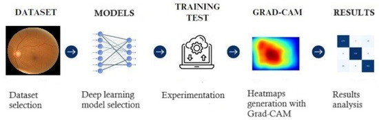
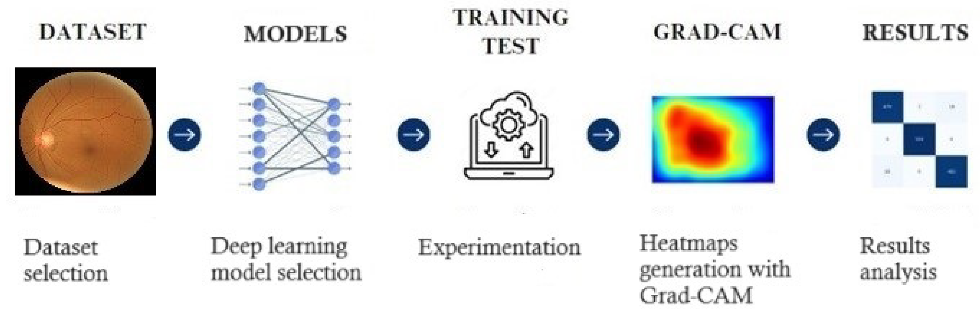
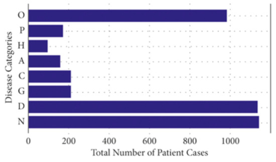
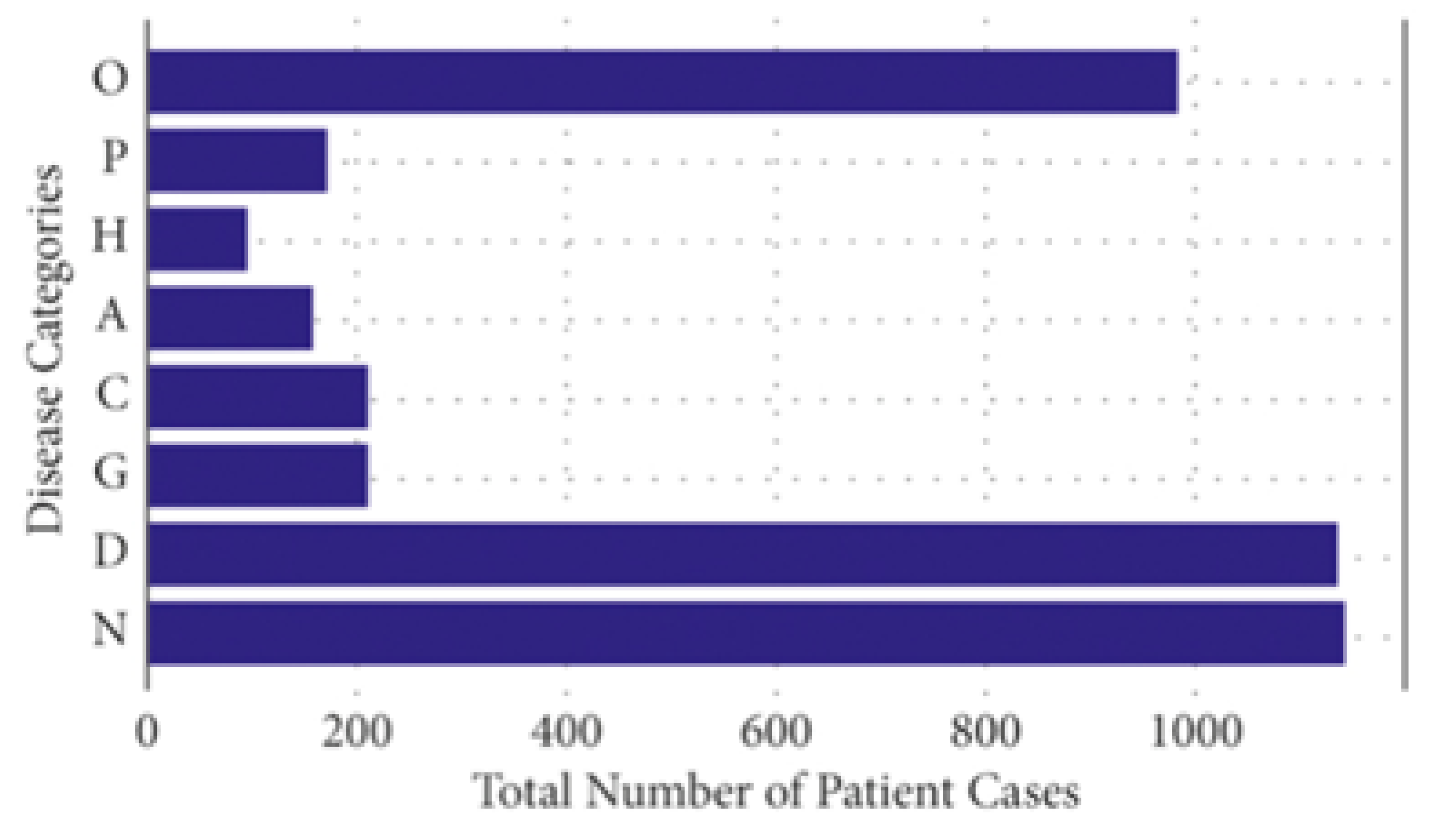
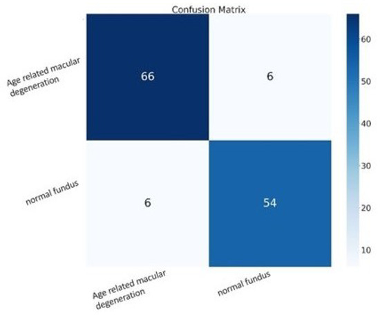
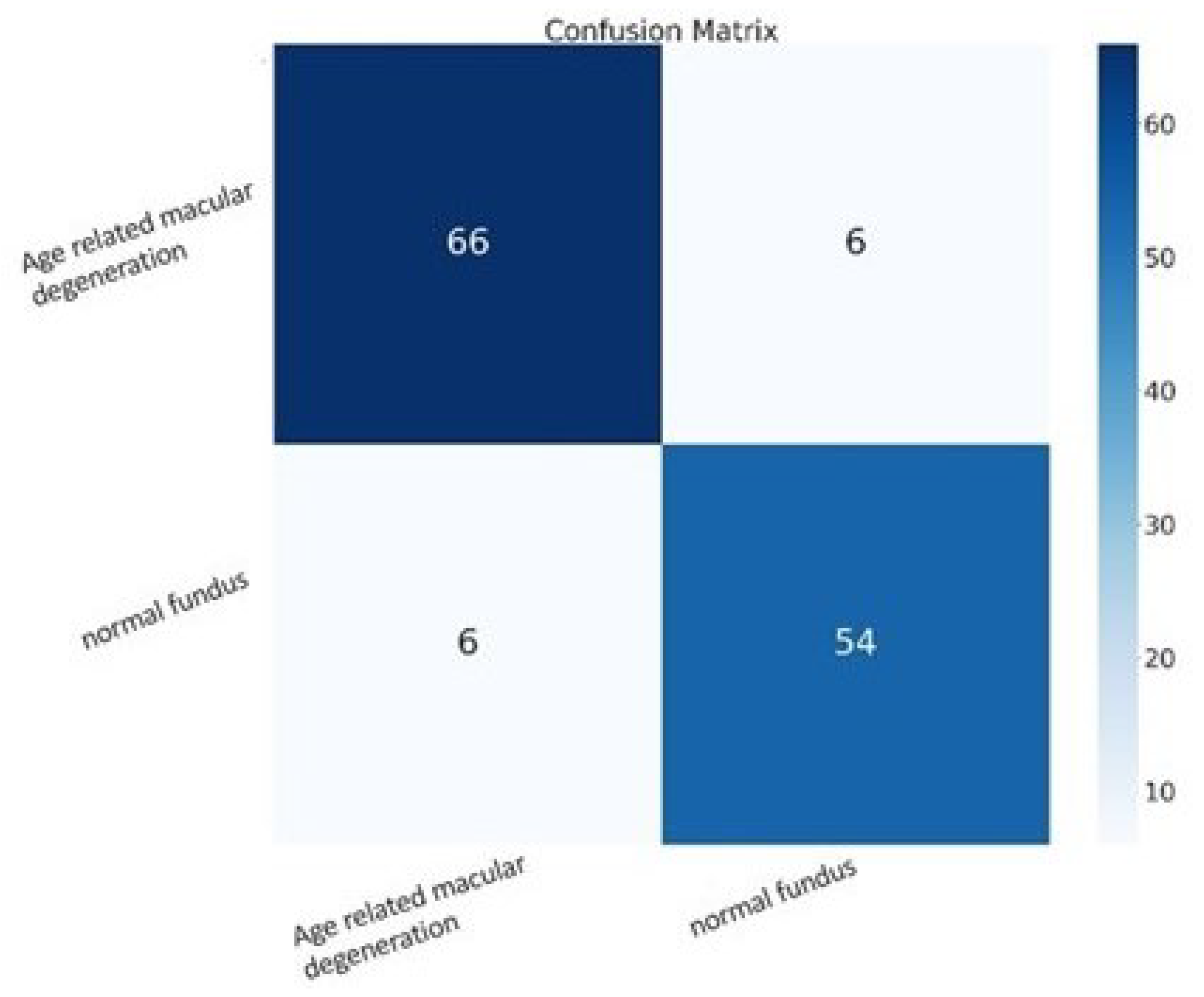
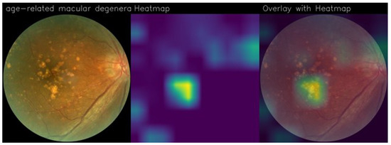
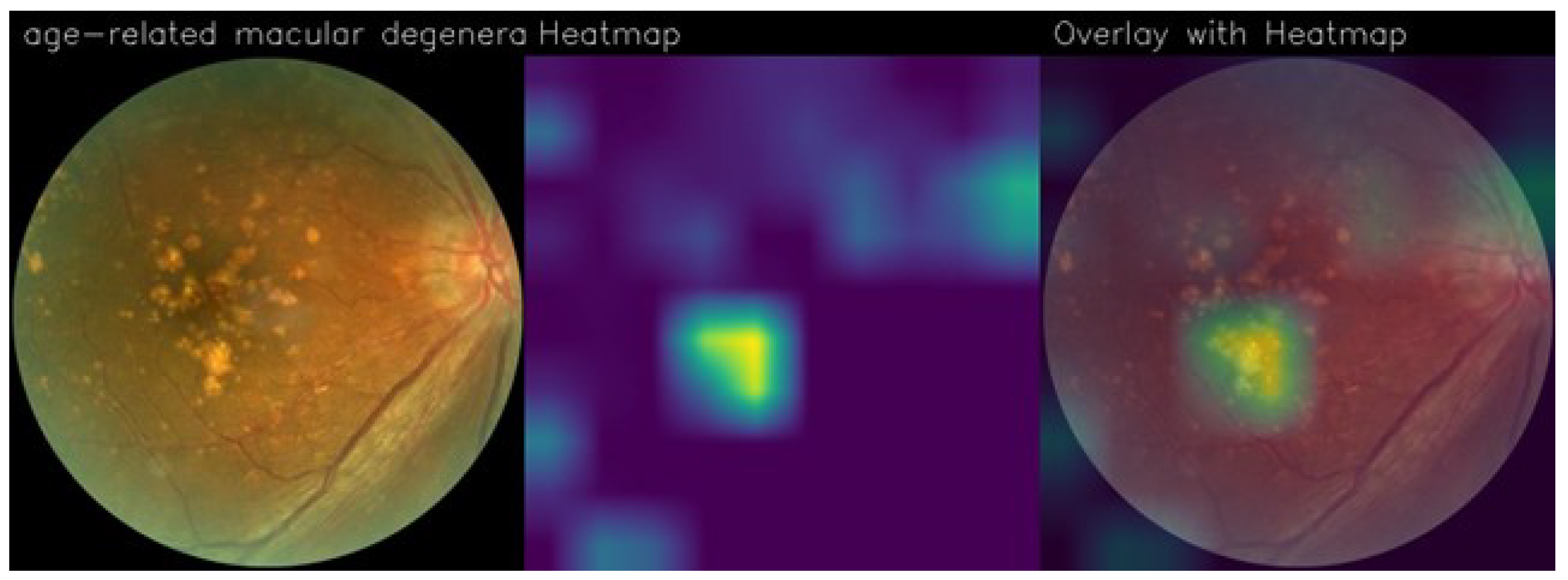
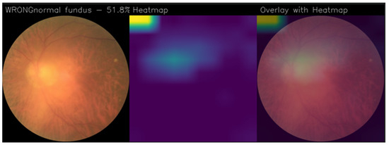
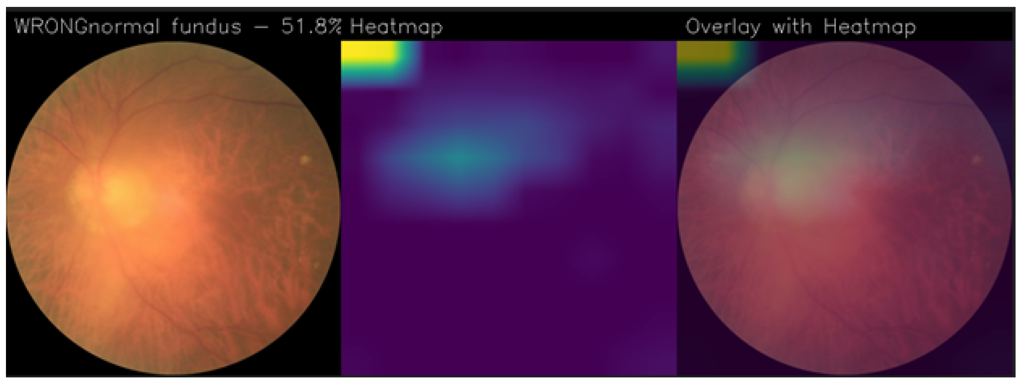
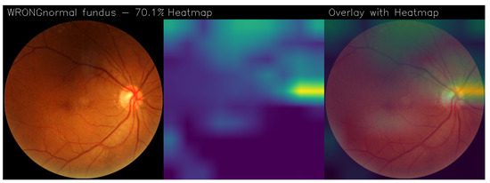
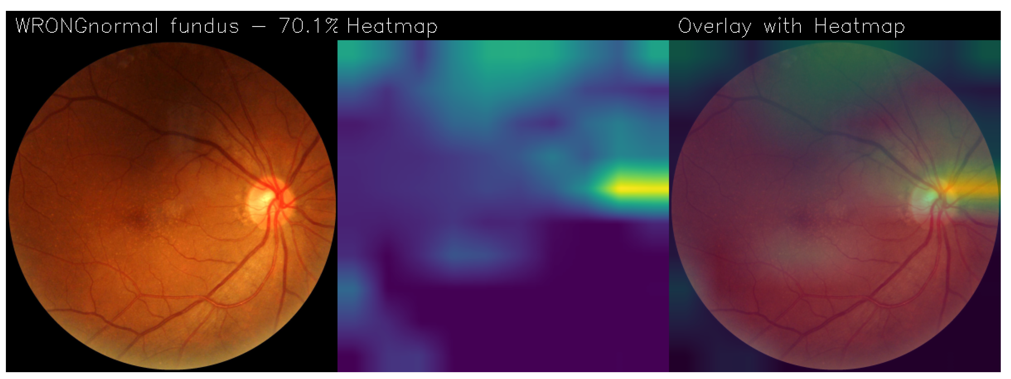
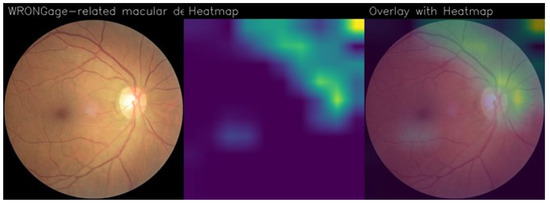
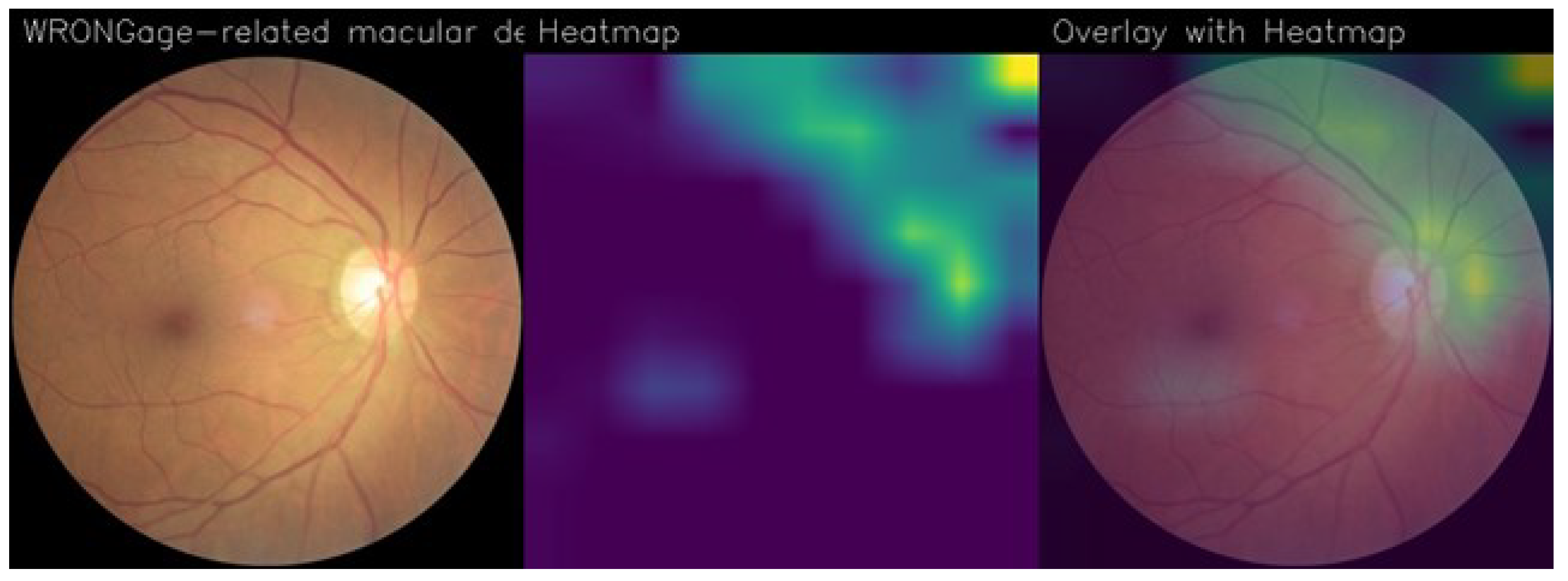
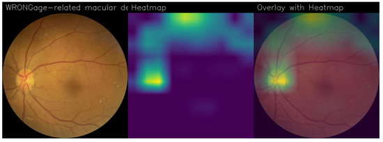
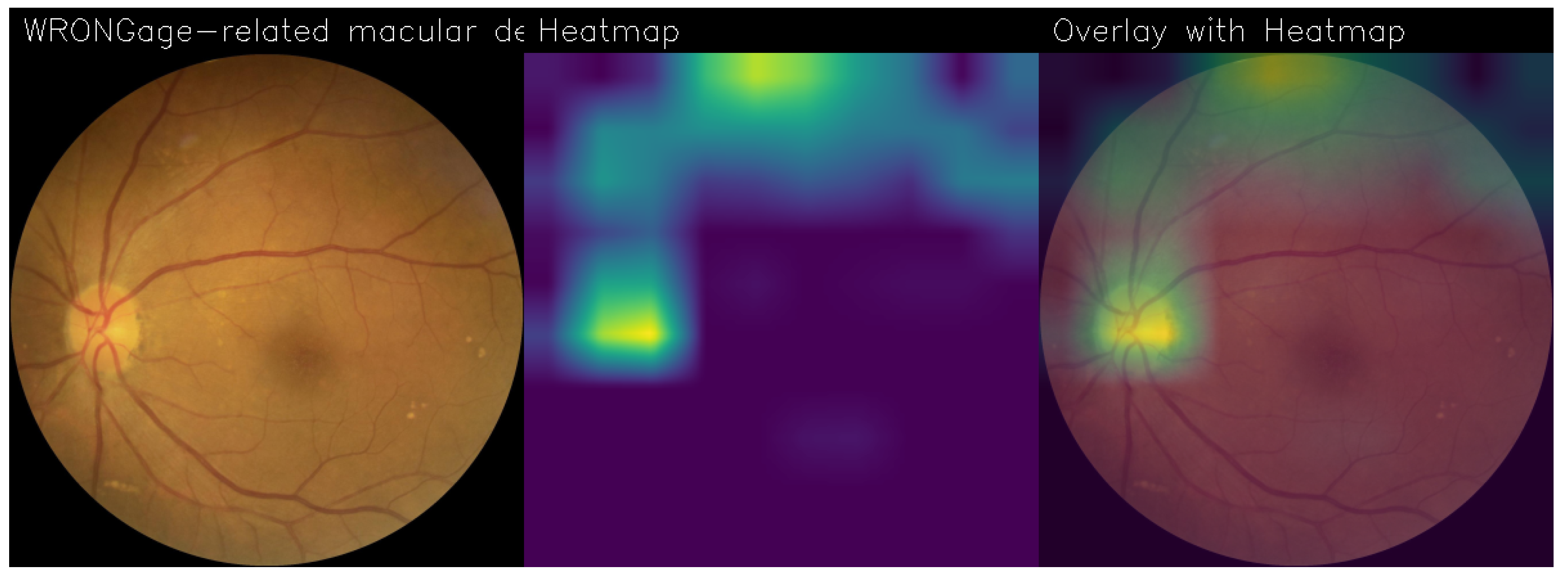
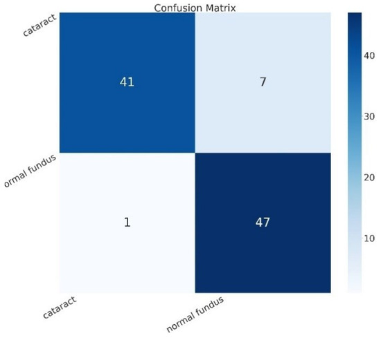
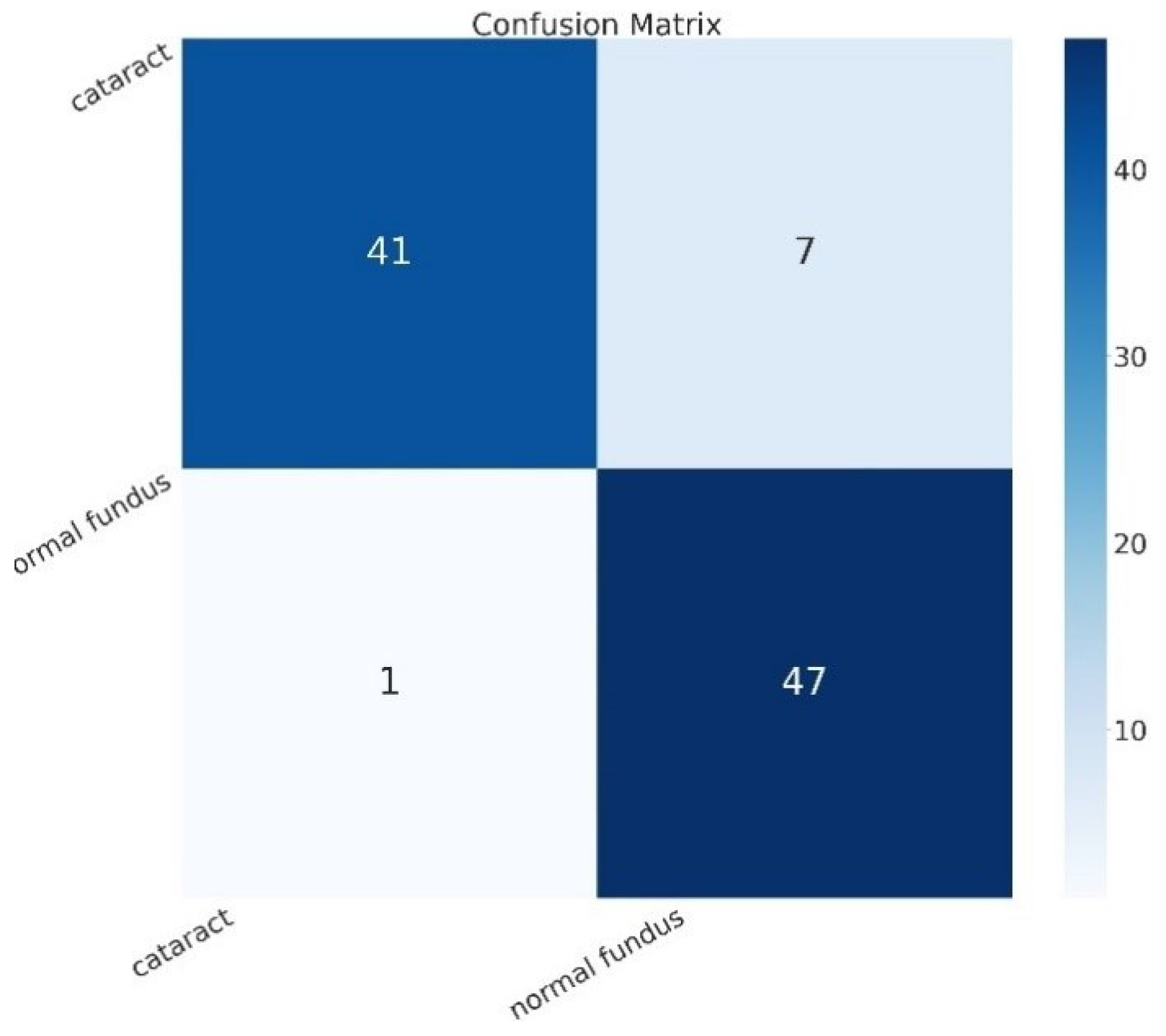
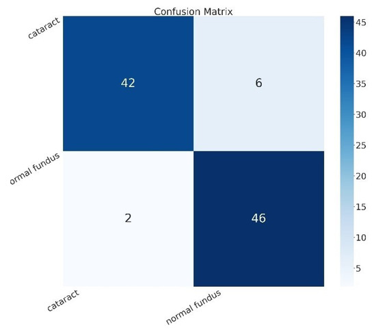
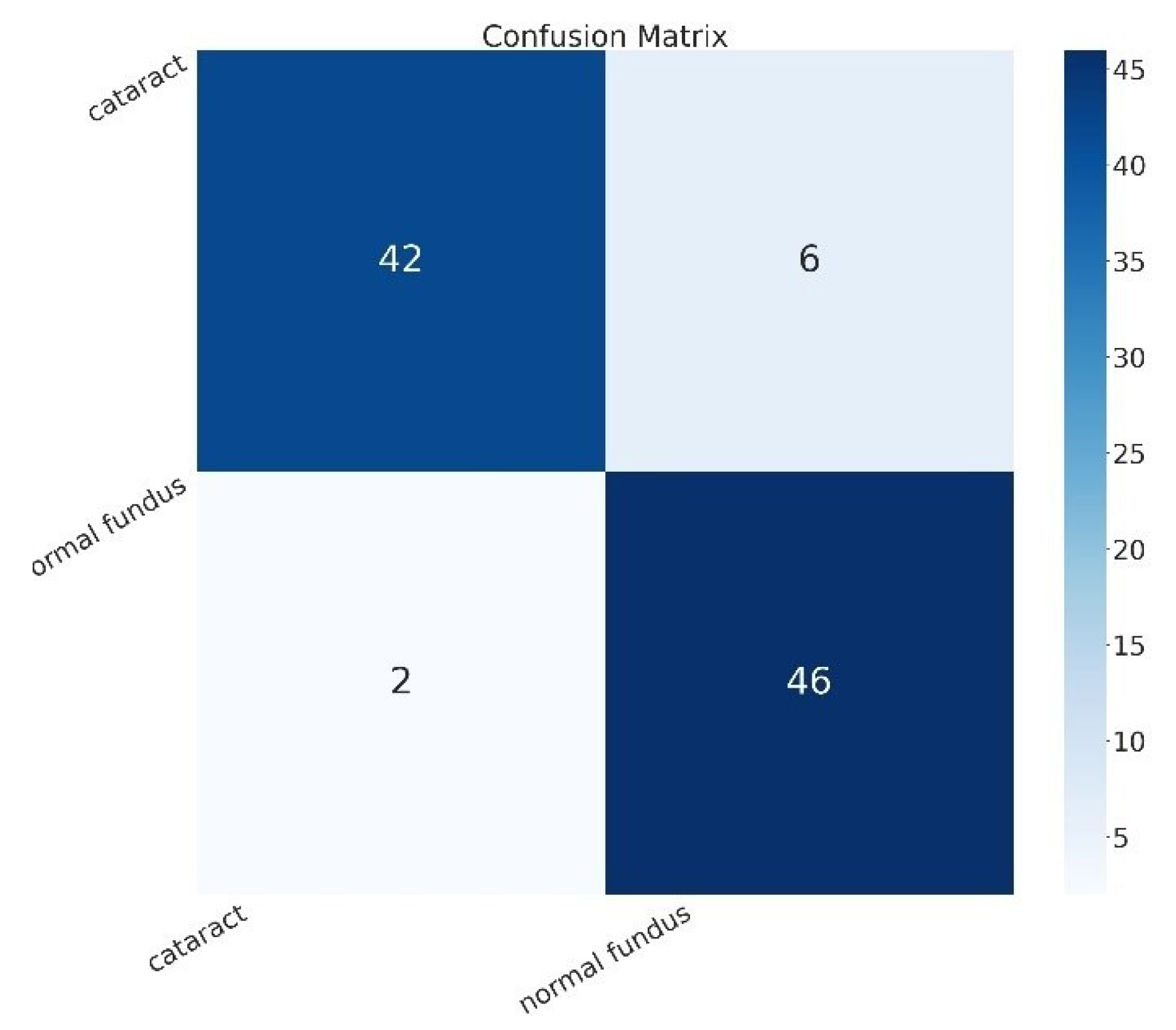
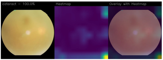
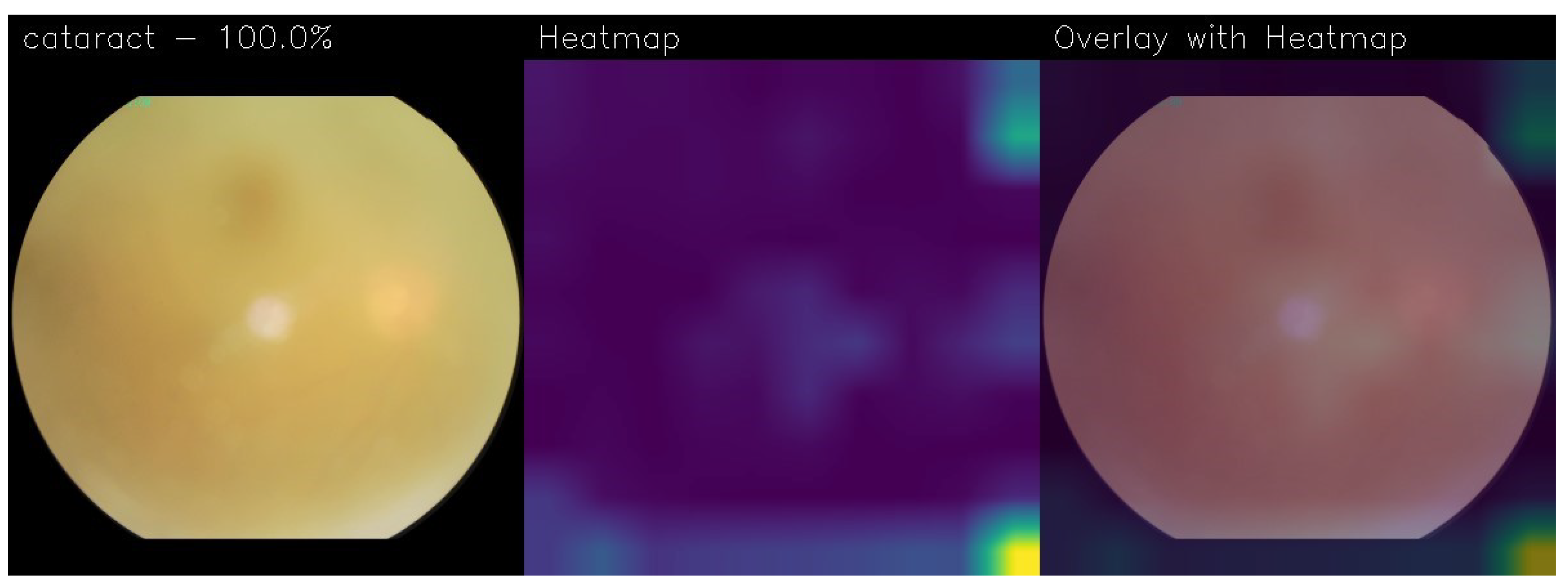
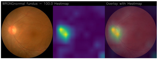
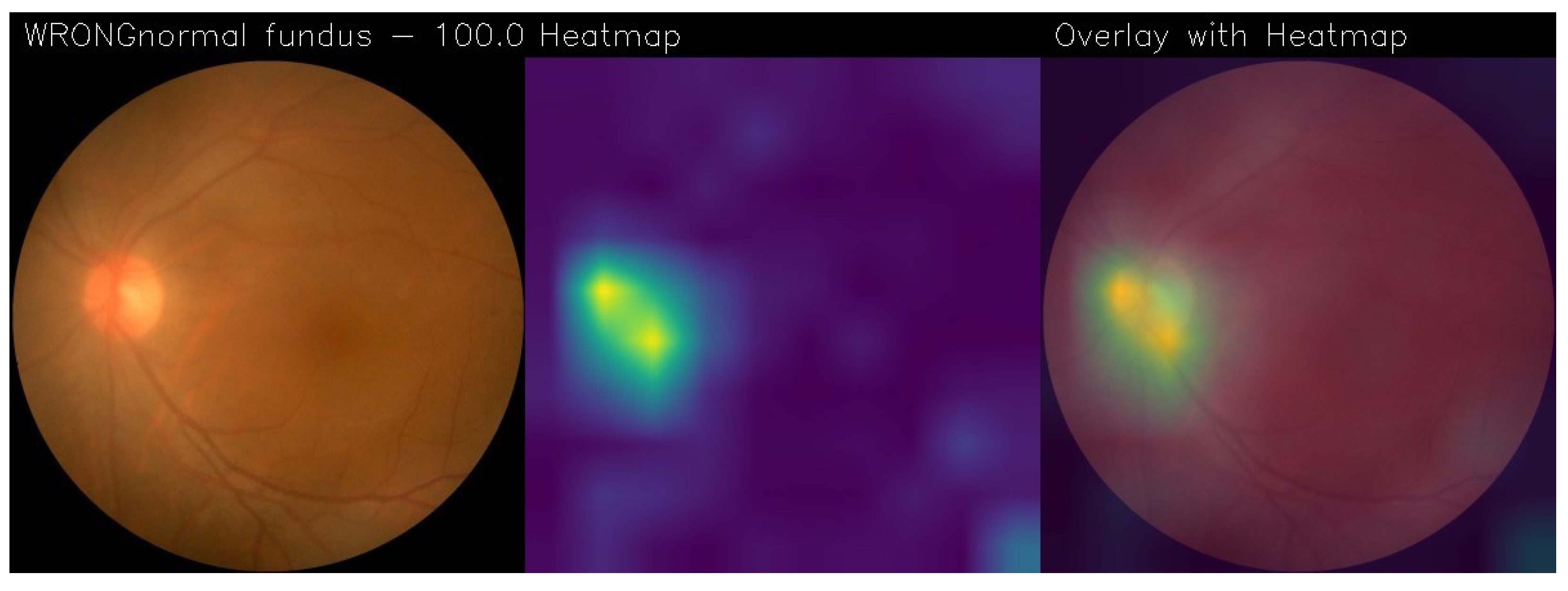
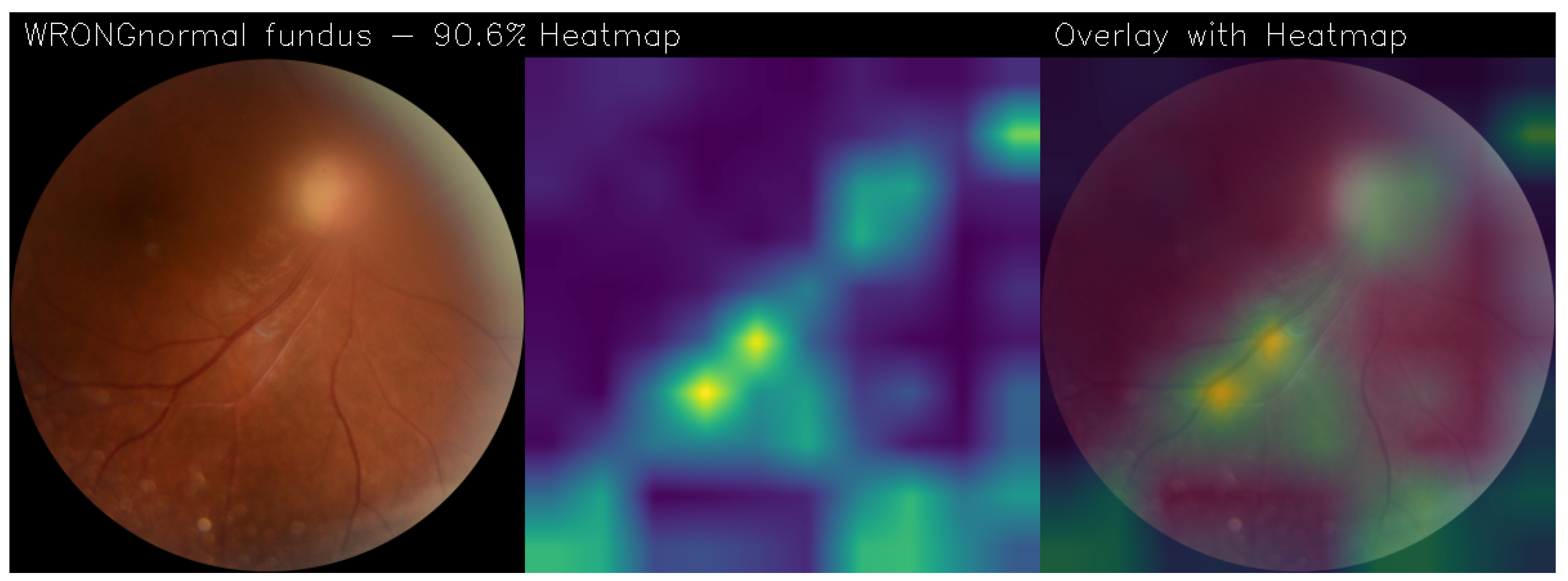
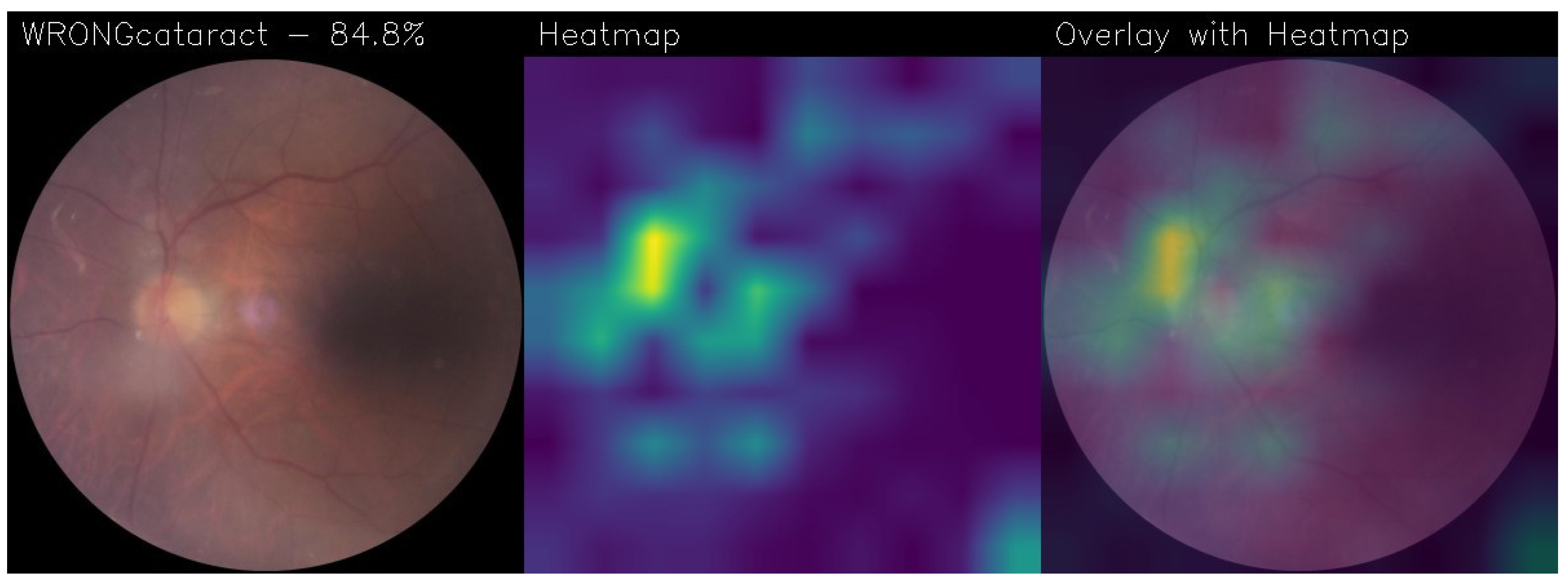
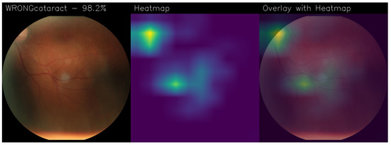
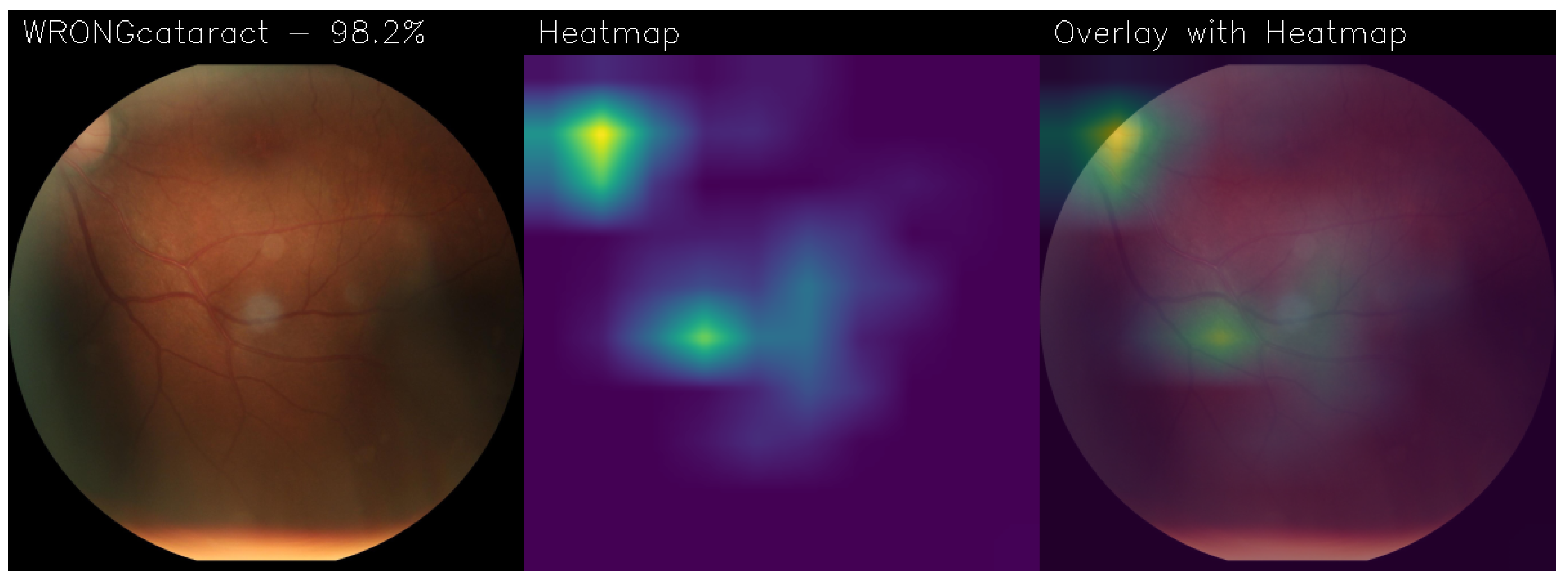
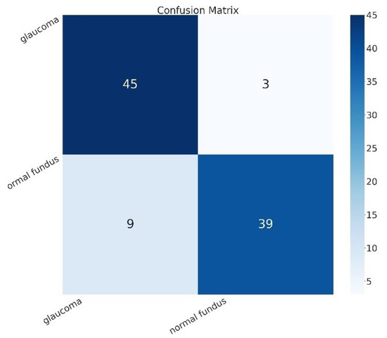
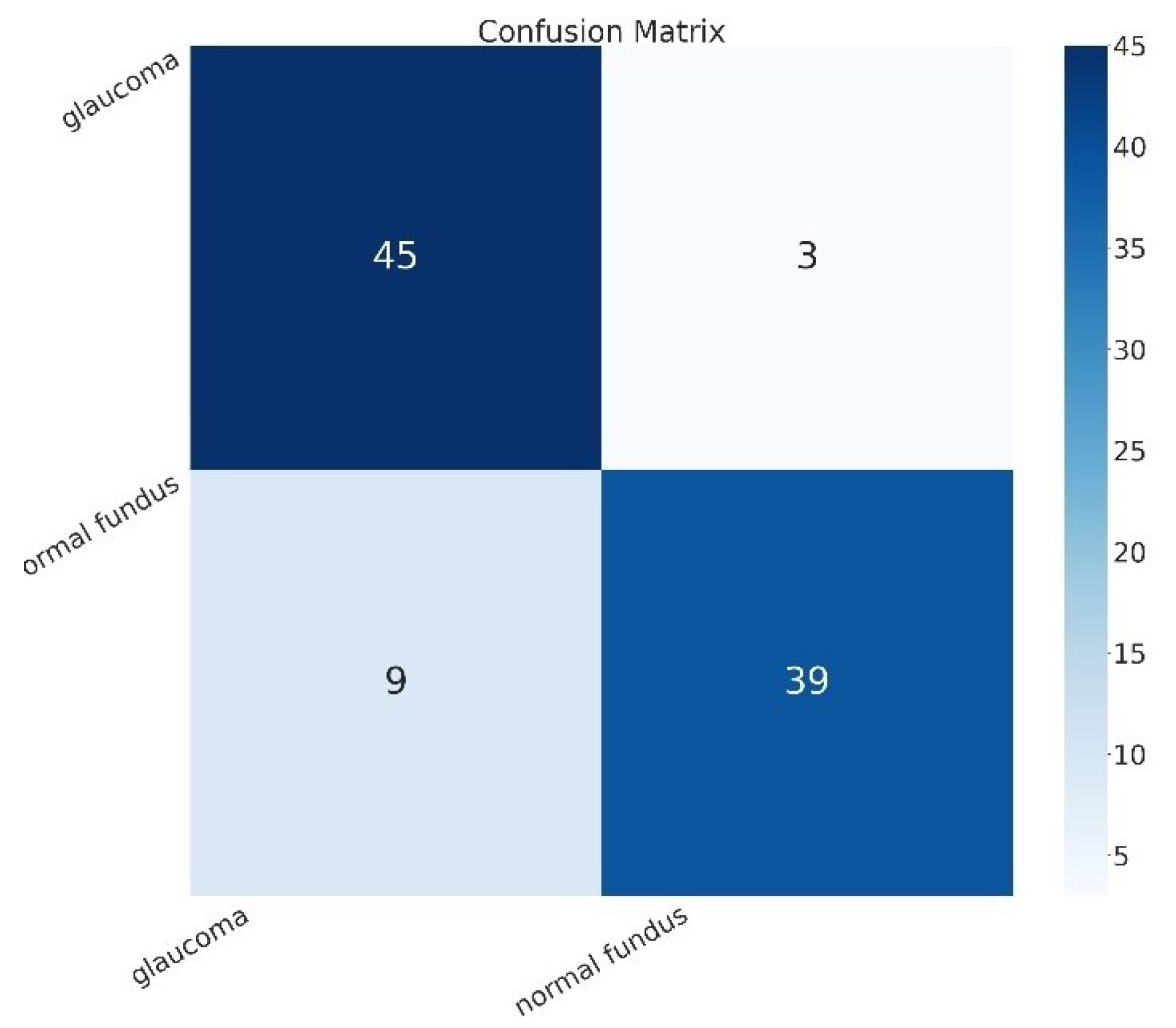
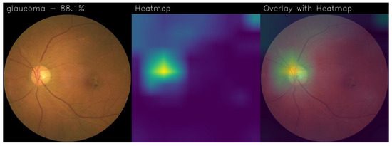
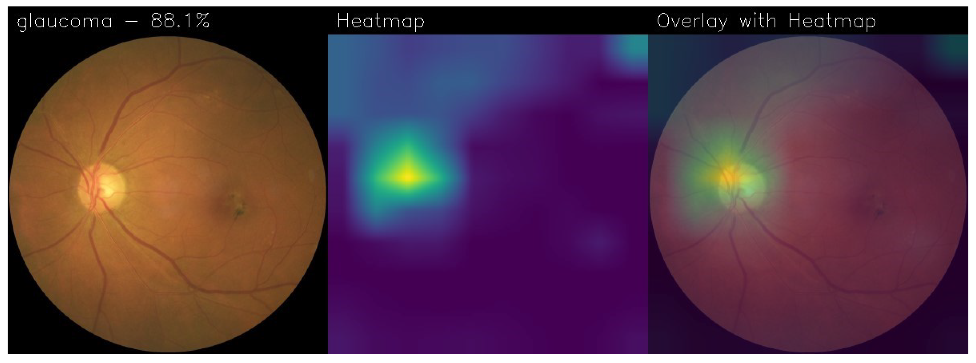
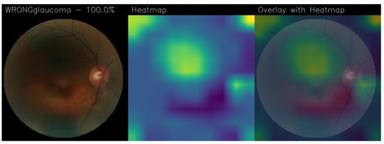
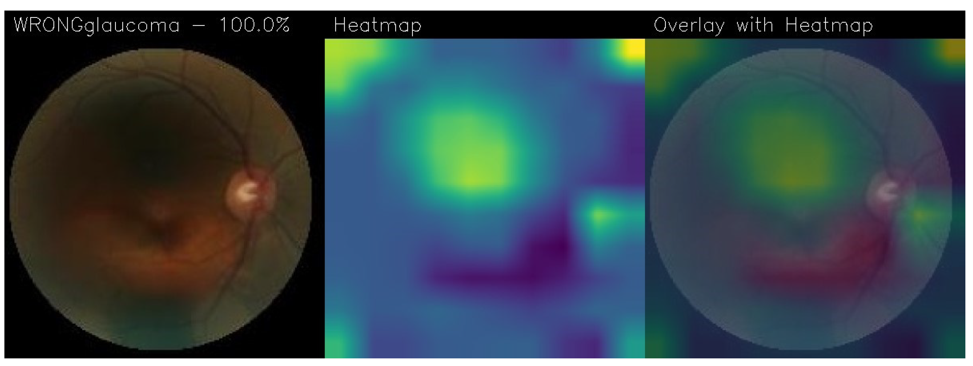
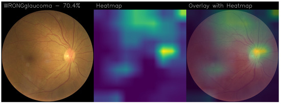
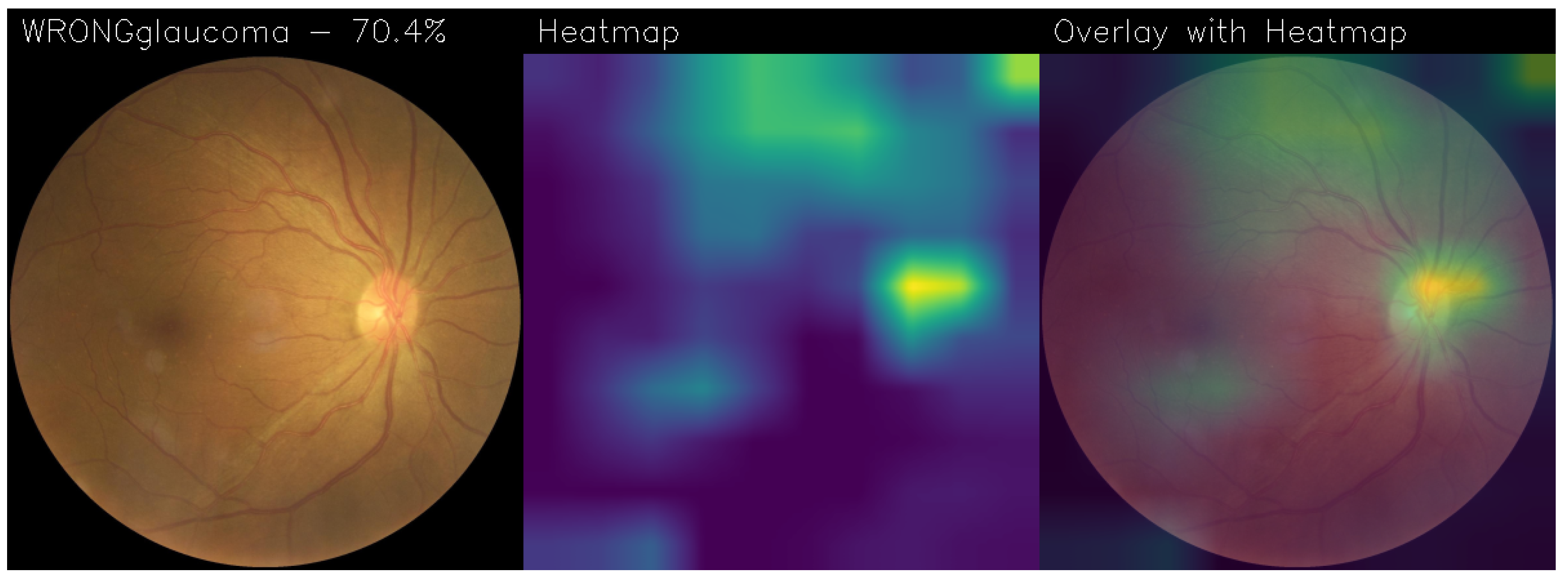
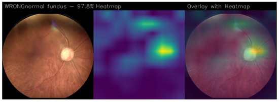
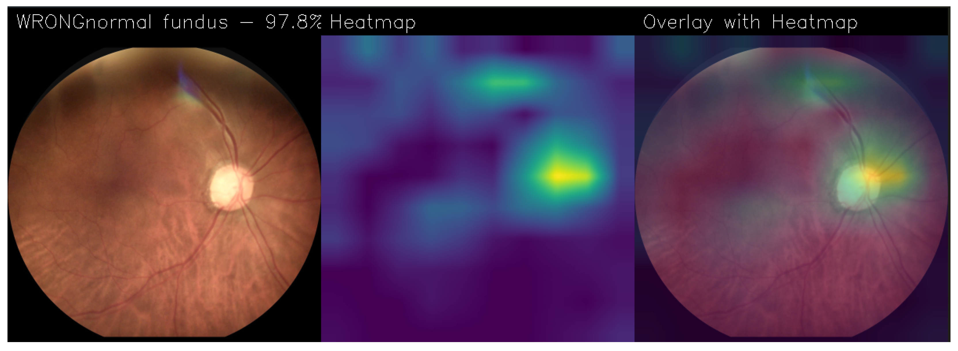
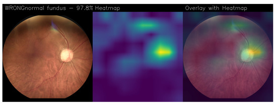
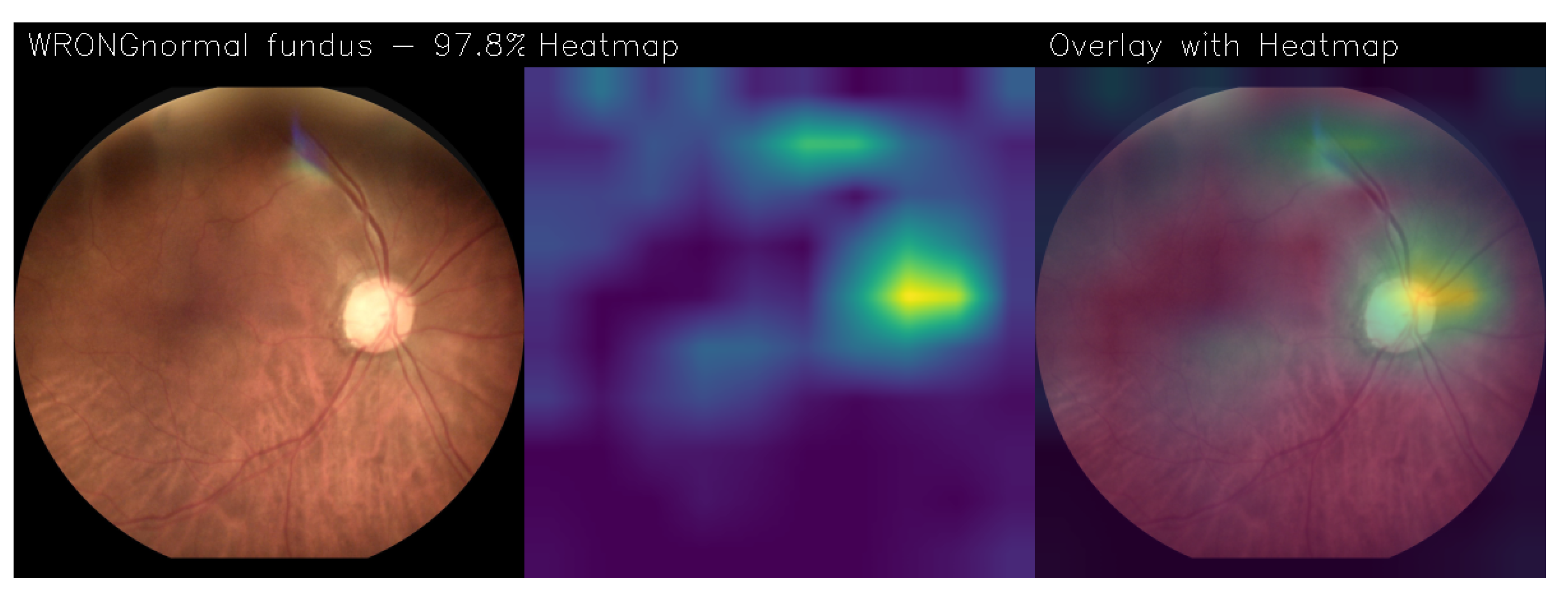
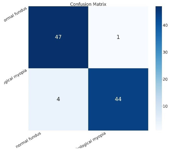
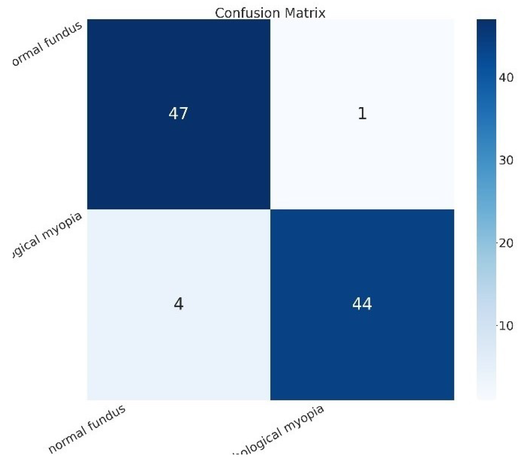
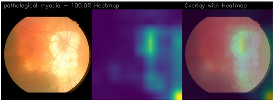
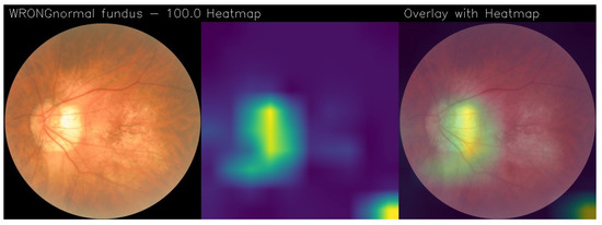
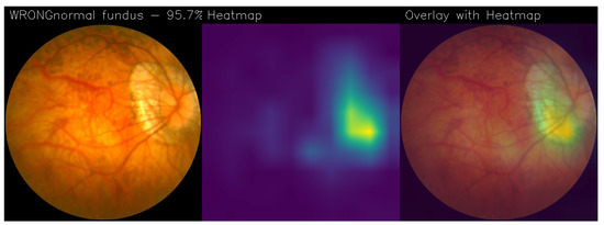
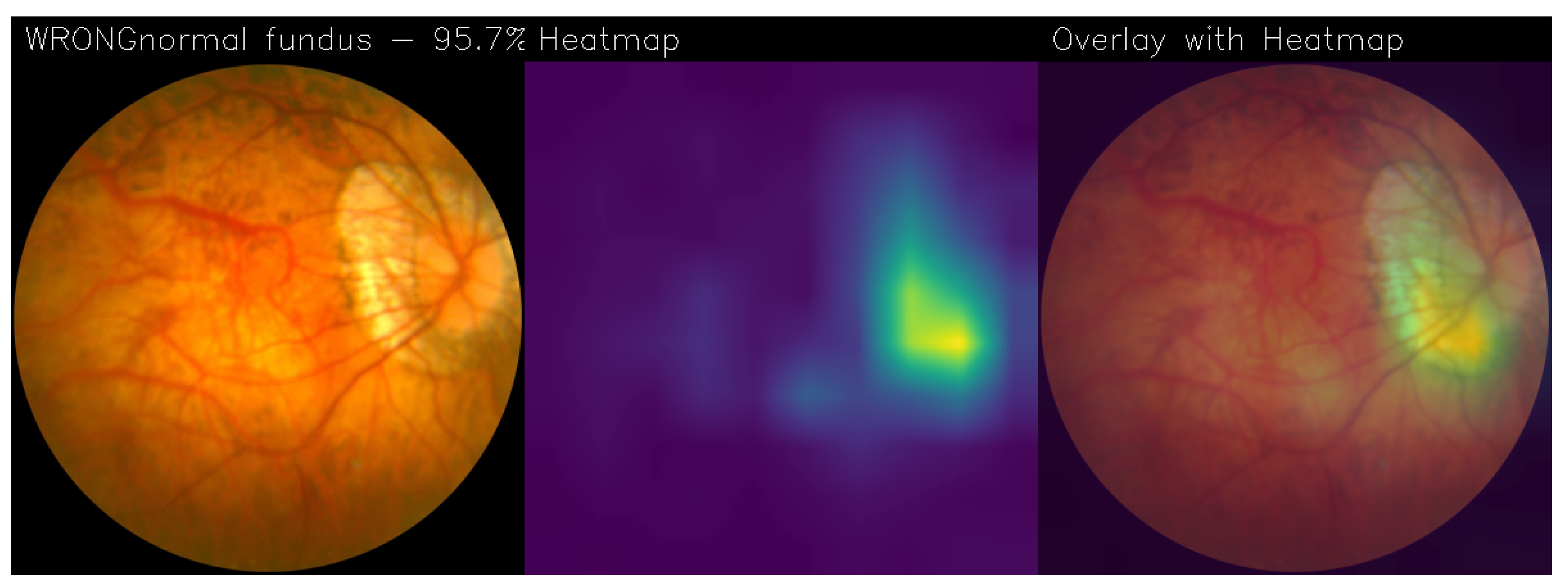
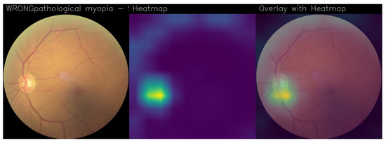
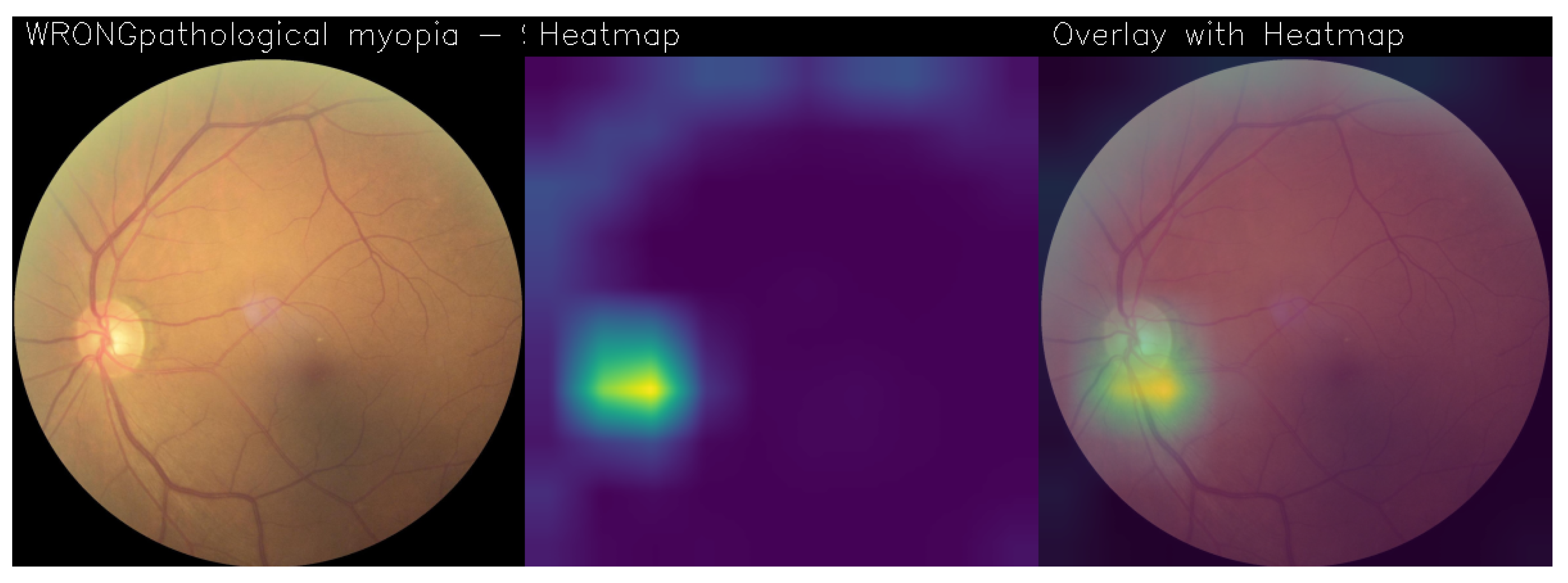

Disclaimer/Publisher’s Note: The statements, opinions and data contained in all publications are solely those of the individual author(s) and contributor(s) and not of MDPI and/or the editor(s). MDPI and/or the editor(s) disclaim responsibility for any injury to people or property resulting from any ideas, methods, instructions or products referred to in the content. |
© 2024 by the authors. Licensee MDPI, Basel, Switzerland. This article is an open access article distributed under the terms and conditions of the Creative Commons Attribution (CC BY) license (https://creativecommons.org/licenses/by/4.0/).