A Systems-Based Superior–Committee Group Decision-Support Method Under Linguistic Intuitionistic Fuzzy Uncertainty

Highlights

Please indicate how your work links to systems science via your contributions to systems practice, theory, and/or methodology.

• A two-stage superior–committee architecture models organizational decision systems in which formal responsibility and advisory expertise remain distinct.
• The framework integrates linguistic uncertainty, input consistency, prior expertise, certainty, agreement, and governance allocation within a unified criteria-weighting methodology.

What are the main findings and/or the implications of the main findings?

• The superior–committee formulation recovered the top criterion in all 300 admissible controlled-validation instances.
• The analyses clarify how expert weighting, inconsistent inputs, subgroup polarization, and the governance coefficient affect the resulting priorities.

Abstract

Decision-making in organizational and socio-technical systems often involves a responsible superior expert who must integrate committee judgments expressed under linguistic uncertainty, hesitation, and heterogeneous expertise. This paper proposes a systems-based superior–committee group decision-support method for criteria weighting under linguistic intuitionistic fuzzy uncertainty. First, the best–worst method is extended by using linguistic intuitionistic fuzzy numbers to represent pairwise preference information with linguistic membership, non-membership, and indeterminacy degrees. A utility transformation is then introduced to convert linguistic intuitionistic fuzzy comparisons into numerical preference values, enabling criteria weights to be derived through linear programming models. Second, a two-stage group decision-support framework is developed for superior–committee decision structures. In the first stage, committee expert influence is calculated by integrating prior expert weights obtained from the superior expert’s evaluation with judgment-derived expert weights based on certainty and agreement. In the second stage, the final criteria weights are obtained by combining the superior expert’s judgments with the weighted committee judgments. A constructed UAV criteria-weighting case and complementary numerical analyses are presented to illustrate the calculation process and examine the behavior of the proposed method. The results show that the framework provides a transparent mechanism for representing uncertain preferences, assigning expert influence, and deriving interpretable criteria weights in superior–committee group decision systems.

1. Introduction

Criteria weighting is central to multi-criteria decision-making (MCDM) because it determines how evaluation information is aggregated and interpreted [1]. Pairwise-comparison methods elicit relative importance directly from decision-makers. The analytic hierarchy process (AHP) requires $n(n-1)/2$ comparisons for n criteria [2]. The best–worst method (BWM) reduces this burden to $2n-3$ comparisons by using the best and worst criteria as references [3,4]. Subsequent studies have examined BWM consistency, priority analysis, analytical formulations, multiplicative models, and methodological developments [5,6,7,8,9,10].

Human judgments nevertheless remain uncertain. Decision-makers may express preferences linguistically, hesitate among adjacent assessments, or provide both supportive and opposing evaluations. Fuzzy, intuitionistic fuzzy, interval-valued intuitionistic fuzzy, stochastic fuzzy, intuitionistic linguistic, and hesitant fuzzy linguistic BWM variants address different aspects of this uncertainty [11,12,13,14,15,16,17,18,19,20,21,22]. Linguistic intuitionistic fuzzy numbers (LIFNs) record linguistic membership, non-membership, and indeterminacy within one assessment [23,24,25,26].

Group decisions add a second challenge. Committee members may differ in prior expertise, certainty, and agreement with other participants [27]. Existing research has developed aggregation, consensus-improvement, compromise-control, trust, and credibility mechanisms under fuzzy linguistic information [28,29,30,31,32]. These mechanisms usually represent the participants as a broadly symmetric group. Organizational decisions often have a different structure: a superior expert retains formal responsibility, while committee experts contribute advisory knowledge.

Table 1 summarizes the resulting methodological gap. Prior research has advanced uncertainty representation, hesitation modeling, group aggregation, consistency analysis, and expert weighting. The unresolved problem is their coordinated use in a role-differentiated structure. Such a structure must distinguish the superior expert’s prior assessment from properties of the current judgments. It must also retain separate superior and committee inputs and control their contributions explicitly.

Table 1. Comparison of representative BWM extensions and related group decision mechanisms.

Approach	Uncertainty Representation	Hesitation Modeling	Expert Weighting	Consensus or Agreement	Authority Structure	Consistency Assessment	Validation Evidence
Conventional BWM [3,4]	Crisp comparison ratios	Not represented	External or equal weights in group applications	Not inherent	Individual or symmetric group roles	Conventional BWM measures	Theory, numerical examples, and applications
Fuzzy BWM [11,12,13]	Triangular or interval-valued fuzzy numbers	Represented through fuzzy spread rather than explicit hesitation	Usually external	Not inherent	Individual or symmetric group roles	Fuzzy consistency measures	Numerical examples and applications
Intuitionistic fuzzy BWM [14,15,16,18,33]	Membership and non-membership degrees	Explicit intuitionistic hesitation	Equal, external, or model-specific	Group aggregation in selected variants	Individual or group roles	Intuitionistic fuzzy consistency measures	Numerical examples and applications
Interval-valued intuitionistic fuzzy BWM [17]	Interval-valued membership and non-membership	Interval-valued hesitation	Not central to the formulation	Not inherent	Individual role	Additive consistency	Numerical analysis
Intuitionistic 2-tuple linguistic BWM [21]	Intuitionistic 2-tuple linguistic assessments	Explicit intuitionistic linguistic hesitation	Not central to the formulation	Not inherent	Individual or group roles	Representation-specific measures	Numerical application
Hesitant fuzzy linguistic BWM [20,22]	Hesitant or double-hierarchy linguistic terms	Multiple possible linguistic terms	Equal or model-specific	Limited	Mainly symmetric group roles	Inconsistency repair or representation-specific measures	Numerical applications
Stochastic fuzzy BWM [19]	Fuzzy scenarios and stochastic comparisons	Scenario uncertainty rather than intuitionistic hesitation	Model-specific	Not inherent	Individual or symmetric group roles	Scenario-based stochastic measures	Numerical and comparative analysis
Group and consensus mechanisms [28,29,30]	Crisp or fuzzy group inputs	Representation-dependent	Equal, prior, or behavior-based	Explicit in selected models	Usually symmetric participation	Constituent or group measures	Case and simulation studies
Proposed linguistic intuitionistic fuzzy BWM (LIF-BWM)	LIFNs with membership and non-membership terms	Indeterminacy retained in LIFNs and incorporated through entropy	Prior and judgment-derived	Similarity-based agreement	Explicit superior and committee roles	Input-based $C{R}_I$ screening, separate from optimized residuals	Constructed case, controlled numerical analysis, benchmarks, ablation, and stress tests

This paper addresses the gap through a two-stage superior–committee LIF-BWM. Stage I integrates the superior expert’s prior evaluation with certainty and agreement derived from the committee’s current judgments. Stage II combines the superior criterion judgments and the weighted committee judgments through the governance coefficient $\mathsf{\Omega }$. The contribution is the integration of these components in a single decision architecture.

The main contributions are as follows:

(1)

LIFNs record linguistic membership, non-membership, and indeterminacy during preference elicitation.

(2)

An explicitly many-to-one utility transformation provides numerical ratios for linear weight optimization, while entropy retains indeterminacy in the certainty calculation.

(3)

Committee influence combines prior assessment with judgment-derived certainty and agreement through a multiplicative integration rule.

(4)

The final model preserves the distinct roles of the superior and committee and integrates their residual blocks through an explicit governance coefficient.

The numerical assessment includes a constructed unmanned aerial vehicle (UAV) case, controlled known-weight validation, harmonized fuzzy BWM comparisons, weighting ablation, stress tests, sensitivity analysis, and computational reporting. Section 2 presents the methodology, Section 3 reports the results, Section 4 discusses their implications, and Section 5 concludes the paper.

2. Methodology

2.1. Preliminaries

This subsection reviews linguistic term sets (LTSs), intuitionistic fuzzy sets (IFSs), and linguistic intuitionistic fuzzy sets (LIFSs).

Definition 1 

([34]). Let $S=\{s_0,s_1,s_2,\dots ,s_t\}$ be a finite, ordered, discrete term set with odd cardinality, where t is a positive integer. It is an LTS if the following properties hold for any $s_i,s_j\in S$:

1 

The set is ordered $s_i\ge s_j$ if and only if $i\ge j$, with maximum and minimum operators defined by

(a) 

$max(s_i,s_j)=s_i\iff s_i\ge s_j$;

(b) 

$min(s_i,s_j)=s_i\iff s_i\le s_j$.

2 

The negation operation is $neg\left(s_i\right)=s_j$, where $j=t-i$.

The term set $S=\{s_i\mid i=0,1,2,\dots ,t\}$ is discrete. Following Martínez and Herrera [34] and Zhang [23], intermediate calculations use the continuous set ${\overline{S}}_{[0,t]}=\{s_i\mid i\in [0,t]\}$. A term $s_i\in S$ is original, while $s_i\notin S$ is virtual. Decision-makers provide original terms, and virtual terms arise during calculation.

Definition 2 

([35]). Let X be a finite set. An intuitionistic fuzzy set (IFS) A in X is

$$\begin{array}{c}\hfill A=\{(x,{\mu }_A\left(x\right),{\nu }_A\left(x\right))\mid x\in X\}\end{array}$$

(1)

where ${\mu }_A:X\to [0,1]$ and ${\nu }_A:X\to [0,1]$ are the membership and non-membership functions. They satisfy ${\mu }_A\left(x\right)+{\nu }_A\left(x\right)\le 1$. The hesitation degree is ${\pi }_A\left(x\right)=1-{\mu }_A\left(x\right)-{\nu }_A\left(x\right)$, and $({\mu }_A\left(x\right),{\nu }_A\left(x\right))$ is an intuitionistic fuzzy number (IFN).

Definition 3 

([23]). Let $s_{\mu },s_{\nu }\in {\overline{S}}_{[0,t]}$, where ${\overline{S}}_{[0,t]}=\{s_i\mid i\in [0,t]\}$ is continuous. If $\mu +\nu \le t$, then $\phi =(s_{\mu },s_{\nu })$ is a linguistic intuitionistic fuzzy number (LIFN). The two components represent linguistic membership and non-membership, while $s_{t-\mu -\nu }$ represents linguistic indeterminacy.

Definition 4 

([23]). Let ${\phi }_1=(s_{{\mu }_1},s_{{\nu }_1})$ and ${\phi }_2=(s_{{\mu }_2},s_{{\nu }_2})$ be two LIFNs, and let $\lambda >0$. Their operational rules are

1. 

${\phi }_1\oplus {\phi }_2=\left(s_{{\mu }_1+{\mu }_2-{\displaystyle \frac{{\mu }_1{\mu }_2}{t}}},s_{{\displaystyle \frac{{\nu }_1{\nu }_2}{t}}}\right)$;

2. 

${\phi }_1\otimes {\phi }_2=\left(s_{{\displaystyle \frac{{\mu }_1{\mu }_2}{t}}},s_{{\nu }_1+{\nu }_2-{\displaystyle \frac{{\nu }_1{\nu }_2}{t}}}\right)$;

3. 

$\lambda {\phi }_1=\left(s_{t-t{\left(1-{\displaystyle \frac{{\mu }_1}{t}}\right)}^{\lambda }},s_{t{\left({\displaystyle \frac{{\nu }_1}{t}}\right)}^{\lambda }}\right)$;

4. 

${\phi }_1^{\lambda }=\left(s_{t{\left({\displaystyle \frac{{\mu }_1}{t}}\right)}^{\lambda }},s_{t-t{\left(1-{\displaystyle \frac{{\nu }_1}{t}}\right)}^{\lambda }}\right)$.

Definition 5 

([23]). For an LIFN $\phi =(s_{\mu },s_{\nu })$, the score function is

$$\begin{array}{c}\hfill S\left(\phi \right)=s_{{\displaystyle \frac{t+\mu -\nu }{2}}}\end{array}$$

(2)

and the accuracy function is

$$\begin{array}{c}\hfill H\left(\phi \right)=s_{\mu +\nu }\end{array}$$

(3)

Definition 6 

([23]). Let ${\phi }_1=(s_{{\mu }_1},s_{{\nu }_1})$ and ${\phi }_2=(s_{{\mu }_2},s_{{\nu }_2})$ be two LIFNs. Their ordering is defined as follows:

1. 

If $S\left({\phi }_1\right)>S\left({\phi }_2\right)$, then ${\phi }_1\succ {\phi }_2$.

2. 

If $S\left({\phi }_1\right)=S\left({\phi }_2\right)$, then

(a) 

If $H\left({\phi }_1\right)>H\left({\phi }_2\right)$, then ${\phi }_1\succ {\phi }_2$;

(b) 

If $H\left({\phi }_1\right)=H\left({\phi }_2\right)$, then ${\phi }_1={\phi }_2$.

Definition 7 

([36]). For an LIFN $\phi =(s_{\mu },s_{\nu })$, the entropy measure is

$$\begin{array}{c}\hfill E\left(\phi \right)={\displaystyle \frac{t-|\mu -\nu |+\pi }{t+\pi }}\end{array}$$

(4)

where $\pi =t-\mu -\nu$.

2.2. Linguistic Intuitionistic Fuzzy Best–Worst Method

BWM uses decision-maker preferences to derive criterion weights. Conventional BWM represents these preferences with crisp values, which may omit linguistic uncertainty and hesitation. LIF-BWM instead uses LIFNs during elicitation and converts them to numerical ratios for optimization.

2.2.1. LIF-BWM Steps

The LIF-BWM contains three main phases: (1) identify the reference criteria, (2) determine the preference comparisons, and (3) derive the optimal weights.

First, specify the criteria $\{C_1,C_2,\dots ,C_n\}$ and identify the best and worst criteria. The best criterion is the most important, and the worst criterion is the least important. BWM then compares these two reference criteria with the remaining criteria.

Second, express the comparisons as LIFNs. The best-to-others vector records the preference of $C_B$ over every $C_j$. Its jth element is $v_{Bj}=(s_{{\mu }_{Bj}},s_{{\nu }_{Bj}})$, where ${\mu }_{Bj},{\nu }_{Bj}\in [0,t]$ and ${\mu }_{Bj}+{\nu }_{Bj}\le t$. The vector is

$$\begin{array}{c}\hfill BO=(v_{B1},v_{B2},\dots ,v_{Bn})\end{array}$$

(5)

where $v_{Bj}=(s_{{\mu }_{Bj}},s_{{\nu }_{Bj}})$ denotes the LIF preference of the best criterion $C_B$ over the jth criterion $C_j$. By definition, $v_{BB}=(s_0,s_t)$.

The others-to-worst vector records the preference of each $C_j$ over $C_W$. Its jth element is $v_{jW}=(s_{{\mu }_{jW}},s_{{\nu }_{jW}})$, where ${\mu }_{jW},{\nu }_{jW}\in [0,t]$ and ${\mu }_{jW}+{\nu }_{jW}\le t$. The vector is

$$\begin{array}{c}\hfill OW=(v_{1W},v_{2W},\dots ,v_{nW})\end{array}$$

(6)

where $v_{jW}=(s_{{\mu }_{jW}},s_{{\nu }_{jW}})$ denotes the LIF preference of the jth criterion $C_j$ over the worst criterion $C_W$. By definition, $v_{WW}=(s_0,s_t)$.

Third, derive the criterion weights. For crisp comparisons, conventional BWM minimizes the largest absolute deviation between the weight ratios and the elicited ratios,

$$\begin{array}{c}minmax\left\{\left|{\displaystyle \frac{{\omega }_B}{{\omega }_j}}-v_{Bj}\right|,\left|{\displaystyle \frac{{\omega }_j}{{\omega }_W}}-v_{jW}\right|\right\}\\ s.t.\left\{\begin{array}{c}{\displaystyle \sum _{j=1}^n}{\omega }_j=1\\ 0\le {\omega }_j\le 1,j=1,2,\dots ,n\end{array}\right.\end{array}$$

(7)

where ${\omega }_j$ denotes the weight of the jth criterion $C_j(j=1,2,\dots ,n)$.

The LIFNs in (7) require numerical representation before they enter a crisp optimization model. Equation (2) gives the linguistic score $s_{(t+\mu -\nu )/2}\in {\overline{S}}_{[0,t]}$. To align its subscript with the conventional BWM scale from 1 to 9, define

$$\begin{array}{c}\hfill U\left(\phi \right)={\displaystyle \frac{t+\mu -\nu }{2}}+1\end{array}$$

(8)

The transformation is many-to-one because it depends on $\mu -\nu$; LIFNs with the same net preference therefore produce the same ratio in the linear program (LP). The entropy-based certainty calculation uses the original LIFNs, including their hesitation information. Based on (7), the LIF-BWM model is

$$\begin{array}{c}min\xi \\ s.t.\left\{\begin{array}{c}\left|{\omega }_B-U\left(v_{Bj}\right){\omega }_j\right|\le \xi \\ \left|{\omega }_j-U\left(v_{jW}\right){\omega }_W\right|\le \xi \\ {\displaystyle \sum _{j=1}^n}{\omega }_j=1\\ 0\le {\omega }_j\le 1,j=1,2,\dots ,n\end{array}\right.\end{array}$$

(9)

where $U\left(v_{Bj}\right)$ and $U\left(v_{jW}\right)$ denote the utility values of $v_{Bj}$ and $v_{jW}$, respectively, such that

$$\begin{array}{c}U\left(v_{Bj}\right)={\displaystyle \frac{t+{\mu }_{Bj}-{\nu }_{Bj}}{2}}+1\\ U\left(v_{jW}\right)={\displaystyle \frac{t+{\mu }_{jW}-{\nu }_{jW}}{2}}+1\end{array}$$

(10)

The absolute-value constraints in model (9) are linearized by replacing each constraint $\left|a\right|\le \xi$ with the two inequalities $a\le \xi$ and $-a\le \xi$. An optimal weight vector ${\omega }^{\ast }={({\omega }_1^{\ast },{\omega }_2^{\ast },\dots ,{\omega }_n^{\ast })}^T$ can be obtained by solving model (9).

2.2.2. Consistency Assessment for LIF-BWM

Consistency is screened from the elicited comparisons before optimization. The perturbation used to derive the consistency index is distinct from the optimized residual in (9). Let $a_{BW}=U\left(v_{BW}\right)$ and denote the preference-scale perturbation by $\delta$. The limiting relation is

$${(a_{BW}-\delta )}^2=a_{BW}+\delta ,$$

(11)

which expands to

$${\delta }^2-(2a_{BW}+1)\delta +(a_{BW}^2-a_{BW})=0.$$

(12)

The admissible root is

$$C{I}_{\delta }\left(a_{BW}\right)={\displaystyle \frac{2a_{BW}+1-\sqrt{8a_{BW}+1}}{2}}.$$

(13)

This quantity lies on the preference scale, whereas ${\xi }^{\ast }$ in (9) lies on the normalized weight scale. Input screening therefore uses $C{R}_I$ below, while ${\xi }^{\ast }$ measures optimized weight fit.

Let $a_{Bj}=U\left(v_{Bj}\right)$ and $a_{jW}=U\left(v_{jW}\right)$. Multiplicative consistency requires $a_{Bj}{a}_{jW}=a_{BW}$ for every criterion. Following the input-based BWM indicator [5], the local and overall consistency ratios are

$$\begin{array}{cc}\hfill C{R}_{Ij}& ={\displaystyle \frac{\left|a_{Bj}{a}_{jW}-a_{BW}\right|}{a_{BW}^2-a_{BW}}},\hfill \\ \hfill C{R}_I& =\underset{j}{max}C{R}_{Ij},\hfill \end{array}$$

(14)

For $a_{BW}>1$, $C{R}_I$ is evaluated against a threshold calibrated jointly to the number of items and the attainable utility scale. Because $U(·)$ generates half-step utilities, calibration is performed on $G_{0.5}\left(m\right)=\{1,1.5,\dots ,m\}$. The threshold $\tau (n,m)$ is defined by the equal-error crossing between ordinal-consistent and ordinal-inconsistent systems on this grid. For each judgment vector, $m=a_{BW}$; hence, the applicable threshold is $\tau (n,a_{BW})$, and the vector is admissible when $C{R}_I\le \tau (n,a_{BW})$.

2.3. Two-Stage Group LIF-BWM

Consider a decision-making problem with n criteria evaluated by l committee experts and one superior expert. The committee experts are denoted by $E_i$$(i=1,2,\dots ,l)$, and criteria are denoted by $C_j$$(j=1,2,\dots ,n)$.

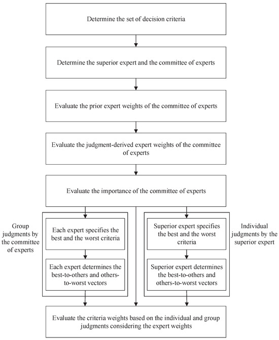
The method has two stages. Stage I determines committee influence from prior assessment, certainty, and judgment agreement. Stage II integrates the superior and weighted committee criterion judgments. Figure 1 demonstrates the process of the proposed method.

Figure 1. Process of the proposed method.

The superior expert supplies the prior expertise assessment, and $\mathsf{\Omega }$ controls the relative contributions of the two judgment blocks in Stage II.

2.3.1. Expert-Weight Calculation

Committee influence includes prior and judgment-derived components. The superior expert’s evaluation determines the prior weights. Entropy and similarity among fitted criterion-weight vectors determine certainty and judgment agreement, respectively. These quantities describe the current judgments and complement the prior expertise assessment. The calculation proceeds as follows.

Step 1: The superior expert identifies the best committee expert $E_B$ (the most knowledgeable) and the worst committee expert $E_W$ (the least knowledgeable).

Step 2: Elicit and screen the superior expert’s LIF-BWM judgments for the prior committee weights.

Step 2-1: Express the preference of the best expert $E_B$ over each committee expert $E_i$ as $f_{Bi}=(s_{{\mu }_{f_{Bi}}},s_{{\nu }_{f_{Bi}}})$. The best-to-others vector is defined below.

$$\begin{array}{c}\hfill F_B=(f_{B1},f_{B2},\dots ,f_{Bl})\end{array}$$

where $f_{Bi}$ represents the preference of $E_B$ over $E_i$. By definition, $f_{BB}=(s_0,s_t)$.

Step 2-2: Express the preference of each $E_i$ over the worst expert $E_W$ as $f_{iW}=(s_{{\mu }_{f_{iW}}},s_{{\nu }_{f_{iW}}})$. The others-to-worst vector is defined below.

$$\begin{array}{c}\hfill F_W=(f_{1W},f_{2W},\dots ,f_{lW})\end{array}$$

where $f_{iW}$ represents the preference of $E_i$ over $E_W$. By definition, $f_{WW}=(s_0,s_t)$.

Step 2-3: Calculate the optimal prior weight vector $({\rho }_1^{\ast },{\rho }_2^{\ast },\dots ,{\rho }_l^{\ast })$ by solving the following model.

$$\begin{array}{c}min\xi \\ s.t.\left\{\begin{array}{c}|{\rho }_B-U\left(f_{Bi}\right){\rho }_i|\le \xi \\ |{\rho }_i-U\left(f_{iW}\right){\rho }_W|\le \xi \\ {\displaystyle \sum _{i=1}^l}{\rho }_i=1\\ 0\le {\rho }_i\le 1,i=1,2,\dots ,l\\ \xi \ge 0\end{array}\right.\end{array}$$

(15)

Step 3: Determine and screen the committee criterion judgments.

Step 3-1: Each committee expert identifies the best criterion $C_{B_i}$ and the worst criterion $C_{W_i}$.

Step 3-2: Expert $E_i$ expresses the preference of $C_{B_i}$ over each $C_j$ as $v_{B_{i}j}^i=(s_{{\mu }_{v_{B_{i}j}^i}},s_{{\nu }_{v_{B_{i}j}^i}})$. The resulting best-to-others vector is defined below.

$$\begin{array}{c}\hfill B{O}^i=(v_{B_{i}1}^i,v_{B_{i}2}^i,\dots ,v_{B_{i}n}^i)\end{array}$$

(16)

Step 3-3: Expert $E_i$ expresses the preference of each $C_j$ over $C_{W_i}$ as $v_{j{W}_i}^i=(s_{{\mu }_{v_{j{W}_i}^i}},s_{{\nu }_{v_{j{W}_i}^i}})$. The resulting others-to-worst vector is defined below.

$$\begin{array}{c}\hfill O{W}^i=(v_{1W_i}^i,v_{2W_i}^i,\dots ,v_{n{W}_i}^i)\end{array}$$

(17)

Step 4: Evaluate each expert’s certainty from the entropy of the $2n-3$ unique BWM comparisons.

$$\begin{array}{c}\hfill {\zeta }_i=1-{\displaystyle \frac{1}{2n-3}}\left({\displaystyle \sum _{\begin{array}{c}j=1\\ j\ne B_i\end{array}}^n}E\left(v_{B_{i}j}^i\right)+{\displaystyle \sum _{\begin{array}{c}j=1\\ j\ne B_i,j\ne W_i\end{array}}^n}E\left(v_{j{W}_i}^i\right)\right)\end{array}$$

(18)

where self-comparisons are excluded and the best-to-worst comparison is counted once. The denominator therefore equals the number of independently elicited BWM judgments. The entropy terms are

$$\begin{array}{c}E\left(v_{B_{i}j}^i\right)={\displaystyle \frac{t-\left|{\mu }_{v_{B_{i}j}^i}-{\nu }_{v_{B_{i}j}^i}\right|+{\pi }_{v_{B_{i}j}^i}}{t+{\pi }_{v_{B_{i}j}^i}}}\\ E\left(v_{j{W}_i}^i\right)={\displaystyle \frac{t-\left|{\mu }_{v_{j{W}_i}^i}-{\nu }_{v_{j{W}_i}^i}\right|+{\pi }_{v_{j{W}_i}^i}}{t+{\pi }_{v_{j{W}_i}^i}}}\end{array}$$

(19)

Step 5: Evaluate judgment agreement among the committee experts.

Step 5-1: Calculate an optimal criterion-weight vector $(w_1^{i\ast },w_2^{i\ast },\dots ,w_n^{i\ast })$ for each expert by solving the following model.

$$\begin{array}{c}min\xi \\ s.t.\left\{\begin{array}{c}|w_{B_i}^i-U\left(v_{B_{i}j}^i\right)w_j^i|\le \xi \\ |w_j^i-U\left(v_{j{W}_i}^i\right)w_{W_i}^i|\le \xi \\ {\displaystyle \sum _{j=1}^n}{w}_j^i=1\\ 0\le w_j^i\le 1,j=1,2,\dots ,n\\ \xi \ge 0\end{array}\right.\end{array}$$

(20)

Step 5-2: Calculate the bounded similarity between $E_i$ and $E_t$ from their criterion-weight vectors.

$$\begin{array}{c}\hfill sim(E_i,E_t)=1-{\displaystyle \frac{1}{2}}{\displaystyle \sum _{j=1}^n}|w_j^{i\ast }-w_j^{t\ast }|\end{array}$$

(21)

Because the weight vectors are probability vectors, $sim(E_i,E_t)\in [0,1]$, where a larger value indicates greater agreement.

Step 5-3: Calculate each expert’s judgment agreement as the average pairwise similarity.

$$\begin{array}{c}\hfill {\eta }_i={\displaystyle \frac{1}{l-1}}{\displaystyle \sum _{\begin{array}{c}t=1\\ t\ne i\end{array}}^l}sim(E_i,E_t)\end{array}$$

(22)

Step 6: Calculate the judgment-derived weight by combining certainty and agreement.

$$\begin{array}{c}\hfill {\lambda }_i=\alpha {\displaystyle \frac{{\zeta }_i}{{\sum }_{k=1}^l{\zeta }_k}}+\left(1-\alpha \right){\displaystyle \frac{{\eta }_i}{{\sum }_{k=1}^l{\eta }_k}},\alpha ={\displaystyle \frac{y_{\zeta }}{y_{\zeta }+y_{\eta }}}\end{array}$$

(23)

where $y_{\zeta }$ and $y_{\eta }$ are the policy allocations assigned to certainty and agreement. They satisfy $y_{\zeta },y_{\eta }\ge 0$ and $y_{\zeta }+y_{\eta }>0$. Thus, $\alpha =1$ uses certainty, $\alpha =0$ uses agreement, and $\alpha =0.5$ assigns equal coefficients to the normalized components.

Step 7: Integrate the prior and judgment-derived weights.

$$\begin{array}{c}\hfill w_i={\displaystyle \frac{{\rho }_i{\lambda }_i}{{\sum }_{k=1}^l{\rho }_k{\lambda }_k}}\end{array}$$

(24)

For strictly positive ${\rho }_i$ and ${\lambda }_i$, (24) is also the unique solution of the entropy-regularized joint-support problem

$$\underset{\mathbf{w}\in {\mathcal{S}}_l}{max}\left\{{\displaystyle \sum _{i=1}^l}{w}_i\left(ln{\rho }_i+ln{\lambda }_i\right)-{\displaystyle \sum _{i=1}^l}{w}_{i}ln{w}_i\right\},{\mathcal{S}}_l=\left\{w:w_i\ge 0,{\displaystyle \sum _{i=1}^l}{w}_i=1\right\}.$$

(25)

The first-order conditions give $w_i\propto {\rho }_i{\lambda }_i$, and normalization yields (24); the non-negative case follows by continuity.

Remark 1. 

The normalized product in (24) is a conjunctive integration rule. Its pairwise ratio is $w_i/w_k=({\rho }_i/{\rho }_k)({\lambda }_i/{\lambda }_k)$. Both components must therefore support a large integrated weight. Section 3 compares this rule with equal, prior-only, judgment-derived-only, and additive weighting.

2.3.2. Criterion-Weight Calculation

The final criterion-weight calculation uses two judgment blocks. The superior block is retained separately, while the committee block incorporates the integrated expert weights. The calculation proceeds as follows.

Step 1: Elicit and screen the superior expert’s LIF-BWM judgments.

Step 1-1: The superior expert identifies the best criterion $C_{B^E}$ and the worst criterion $C_{W^E}$.

Step 1-2: The superior expert expresses the preference of $C_{B^E}$ over each $C_j$ as $e_{B^{E}j}$. Its components are $s_{{\mu }_{e_{B^{E}j}}}$ and $s_{{\nu }_{e_{B^{E}j}}}$. The best-to-others vector is defined below.

$$\begin{array}{c}\hfill E_{BO}=(e_{B^{E}1},e_{B^{E}2},\dots ,e_{B^{E}n})\end{array}$$

The LIFN $e_{B^{E}j}$ denotes the preference of the superior expert’s best criterion $C_{B^E}$ over the jth criterion $C_j$. By definition, $e_{B^E{B}^E}=(s_0,s_t)$.

Step 1-3: The superior expert expresses the preference of each $C_j$ over $C_{W^E}$ as $e_{j{W}^E}$. Its components are $s_{{\mu }_{e_{j{W}^E}}}$ and $s_{{\nu }_{e_{j{W}^E}}}$. The others-to-worst vector is defined below.

$$\begin{array}{c}\hfill E_{OW}=(e_{1W^E},e_{2W^E},\dots ,e_{n{W}^E})\end{array}$$

The LIFN $e_{j{W}^E}$ denotes the preference of the jth criterion $C_j$ over the superior expert’s worst criterion $C_{W^E}$. By definition, $e_{W^E{W}^E}=(s_0,s_t)$.

Step 2: Elicit and screen the committee experts’ LIF-BWM judgments.

Step 2-1: Each expert identifies the best and worst criteria.

Step 2-2: Each expert supplies an LIFN best-to-others vector as defined in (16).

Step 2-3: Each expert supplies an LIFN others-to-worst vector as defined in (17).

Step 3: Calculate the optimal criterion weights $({\omega }_1^{\ast },{\omega }_2^{\ast },\dots ,{\omega }_n^{\ast })$ using the following model.

$$\begin{array}{c}min\left\{\begin{array}{c}\mathsf{\Omega }\underset{j}{\max }\left\{|{\omega }_{B^E}-U\left(e_{B^{E}j}\right){\omega }_j|,|{\omega }_j-U\left(e_{j{W}^E}\right){\omega }_{W^E}|\right\}+\\ \left(1-\mathsf{\Omega }\right){\displaystyle \sum _{i=1}^l}{w}_i\underset{j}{\max }\left\{|{\omega }_{B_i}-U\left(v_{B_{i}j}^i\right){\omega }_j|,|{\omega }_j-U\left(v_{j{W}_i}^i\right){\omega }_{W_i}|\right\}\end{array}\right\}\\ s.t.\left\{\begin{array}{c}{\displaystyle \sum _{j=1}^n}{\omega }_j=1\\ 0\le {\omega }_j\le 1\end{array}\right.\end{array}$$

(26)

where $w_i$ is the integrated weight of $E_i$ obtained in Stage I. Model (26) integrates the superior and committee judgment blocks. Let $g_S$ and $g_C$ denote ex ante allocations to superior authority and committee advice. The governance coefficient is

$$\mathsf{\Omega }={\displaystyle \frac{g_S}{g_S+g_C}},g_S,g_C\ge 0,g_S+g_C>0.$$

(27)

These allocations may be obtained from formal decision rights, an organizational charter, or a direct 100-point allocation before the criterion weights are calculated. Thus, $\mathsf{\Omega }=1$ uses the superior block, $\mathsf{\Omega }=0$ uses the committee block, and $\mathsf{\Omega }=0.5$ assigns equal coefficients to the two blocks. The realized effects may differ because the residual structures and committee weights differ. Prior expert weights operate within the committee block, whereas $\mathsf{\Omega }$ operates between the superior and committee blocks. The two parameters therefore represent different levels of authority. Because experts may select different best and worst criteria, (26) is transformed into the following linear program:

$$\begin{array}{c}min\Delta =\mathsf{\Omega }\xi +(1-\mathsf{\Omega }){\displaystyle \sum _{i=1}^l}{w}_i{\xi }_i\\ s.t.\left\{\begin{array}{c}|{\omega }_{B^E}-U\left(e_{B^{E}j}\right){\omega }_j|\le \xi \\ |{\omega }_j-U\left(e_{j{W}^E}\right){\omega }_{W^E}|\le \xi \\ |{\omega }_{B_i}-U\left(v_{B_{i}j}^i\right){\omega }_j|\le {\xi }_i\\ |{\omega }_j-U\left(v_{j{W}_i}^i\right){\omega }_{W_i}|\le {\xi }_i\\ {\displaystyle \sum _{j=1}^n}{\omega }_j=1\\ 0\le {\omega }_j\le 1,j=1,2,\dots ,n\\ \xi \ge 0,{\xi }_i\ge 0,i=1,2,\dots ,l\end{array}\right.\end{array}$$

(28)

Model (28) is linear. For a specified $\mathsf{\Omega }$, it yields the optimal criterion-weight vector $({\omega }_1^{\ast },{\omega }_2^{\ast },\dots ,{\omega }_n^{\ast })$, the superior residual ${\xi }^{\ast }$, and the committee residuals $({\xi }_1^{\ast },{\xi }_2^{\ast },\dots ,{\xi }_l^{\ast })$.

The objective value ${\Delta }^{\ast }=\mathsf{\Omega }{\xi }^{\ast }+(1-\mathsf{\Omega }){\sum }_{i=1}^l{w}_i{\xi }_i^{\ast }$ is the optimized deviation for the combined judgments under the specified $\mathsf{\Omega }$ and $w$. Input admissibility remains governed by $C{R}_I$ for every constituent vector.

2.3.3. Summary Algorithm

Algorithm 1 summarizes the two-stage procedure.

Algorithm 1 Two-stage group LIF-BWM

Stage I: Expert-weight calculation. Step 1: The superior expert specifies the best expert $E_B$ and the worst expert $E_W$ among the committee members. Step 2: Elicit and screen the superior expert’s best-to-others and others-to-worst vectors.    Use LIF-BWM to calculate the prior committee weights $({\rho }_1^{\ast },{\rho }_2^{\ast },\dots ,{\rho }_l^{\ast })$. Step 3: Determine and screen each committee expert’s LIFN comparison vectors. Step 4: Compute the certainty degrees $({\zeta }_1,{\zeta }_2,\dots ,{\zeta }_l)$ for the committee experts using the entropy measure (18). Step 5: Compute the judgment-agreement scores $({\eta }_1,{\eta }_2,\dots ,{\eta }_l)$ using (20)–(22). Step 6: Calculate the judgment-derived weights $({\lambda }_1,{\lambda }_2,\dots ,{\lambda }_l)$ of the committee experts based on certainty and agreement. Step 7: Calculate the integrated weights of the committee experts by combining the prior and judgment-derived weights. Stage II: Criterion-weight calculation. Step 1: Determine and screen the superior expert’s best-to-others and others-to-worst vectors. Step 2: Determine and screen each committee expert’s best-to-others and others-to-worst vectors. Step 3: Calculate $({\omega }_1^{\ast },{\omega }_2^{\ast },\dots ,{\omega }_n^{\ast })$ by solving (28).

2.3.4. Computational Complexity and Parameter Specification

For n criteria and l committee experts, each participant supplies $2n-3$ criterion comparisons. The criterion assessments therefore require $(l+1)(2n-3)$ comparisons. The superior expert also supplies $2l-3$ comparisons for prior committee weighting. The complete elicitation burden is

$$N_{\mathrm{elicitation}}=(l+1)(2n-3)+(2l-3).$$

(29)

Compared with an equally weighted group BWM involving the same participants, the additional burden is $2l-3$ comparisons.

The main procedure solves one LP for prior committee weights, l individual LIF-BWM models for agreement assessment, and one final LP. It therefore requires $l+2$ LP solutions. Pairwise similarities among the l criterion-weight vectors require $l(l-1)/2$ vector comparisons and $O\left(l^{2}n\right)$ arithmetic operations. All optimization models remain linear.

The coefficients $\alpha$ and $\mathsf{\Omega }$ are specified before the decision results are examined. The allocations $y_{\zeta }$ and $y_{\eta }$ in (23) may be obtained from a direct 100-point allocation between certainty and agreement. The allocations $g_S$ and $g_C$ in (27) may be derived from formal decision rights or an equivalent allocation between superior authority and committee advice. Equal allocations give the equal-allocation reference settings $\alpha =0.5$ and $\mathsf{\Omega }=0.5$. When the policy allocations are imprecise, the corresponding coefficient intervals are evaluated through sensitivity analysis.

The piecewise behavior with respect to $\alpha$ follows from the LP objective. Define normalized certainty and agreement as $z_i={\zeta }_i/{\sum }_k{\zeta }_k$ and $h_i={\eta }_i/{\sum }_k{\eta }_k$. Then ${\lambda }_i\left(\alpha \right)=h_i+\alpha (z_i-h_i)$. Let $a_i={\rho }_i{h}_i$, $b_i={\rho }_i(z_i-h_i)$, $A={\sum }_i{a}_i$, and $B={\sum }_i{b}_i$. For a feasible extreme point r, the objective value is

$$F_r\left(\alpha \right)={\displaystyle \frac{\mathsf{\Omega }{\xi }_S^r(A+\alpha B)+(1-\mathsf{\Omega }){\sum }_i(a_i+\alpha b_i){\xi }_i^r}{A+\alpha B}}.$$

(30)

The feasible region is fixed as $\alpha$ varies. An optimal extreme point therefore remains unchanged until its objective equals that of a competing point. Candidate breakpoints solve

$$\mathsf{\Omega }({\xi }_S^r-{\xi }_S^s)(A+\alpha B)+(1-\mathsf{\Omega })\sum _i(a_i+\alpha b_i)({\xi }_i^r-{\xi }_i^s)=0.$$

(31)

When the denominator is nonzero, the corresponding candidate root is

$${\alpha }_{rs}^{\ast }=-{\displaystyle \frac{\mathsf{\Omega }A({\xi }_S^r-{\xi }_S^s)+(1-\mathsf{\Omega }){\sum }_i{a}_i({\xi }_i^r-{\xi }_i^s)}{\mathsf{\Omega }B({\xi }_S^r-{\xi }_S^s)+(1-\mathsf{\Omega }){\sum }_i{b}_i({\xi }_i^r-{\xi }_i^s)}}.$$

(32)

Only roots in $[0,1]$ that satisfy the neighboring optimality conditions are retained. This calculation explains why $\alpha$ may change ${\Delta }^{\ast }$ continuously while the criterion-weight vector remains constant over an interval.

3. Results

The constructed UAV case presents the complete two-stage calculation with admissible inputs. The subsequent analyses evaluate weight recovery from a known reference vector, compare the methods, and examine ablation, stress tests, parameter sensitivity, and runtime. All calculations use $t=8$. The baseline settings $\alpha =0.5$ and $\mathsf{\Omega }=0.5$ assign equal coefficients to their respective components.

3.1. Constructed UAV Criteria-Weighting Case

The application context and six criteria are adapted from the UAV power-line-inspection study of Gao [37]. The criteria are maximum speed ($C_1$), flight duration ($C_2$), price ($C_3$), maintenance cost ($C_4$), useful life ($C_5$), and operability ($C_6$). The published study supplied the application context and criterion definitions. We constructed the superior–committee structure, latent profiles, LIFN judgments, expert weights, criterion weights, and numerical results for the present analysis. The role-differentiated structure contains one hypothetical superior expert and four hypothetical committee experts; all case inputs and results are author-generated. Table 2 lists the latent priority profiles used in the case.

Table 2. Declared latent priority profiles used to construct the UAV case.

Role	${\mathit{C}}_1$	${\mathit{C}}_2$	${\mathit{C}}_3$	${\mathit{C}}_4$	${\mathit{C}}_5$	${\mathit{C}}_6$
Superior	0.18	0.30	0.15	0.07	0.12	0.18
$E_1$	0.18	0.34	0.07	0.08	0.15	0.18
$E_2$	0.15	0.20	0.30	0.08	0.10	0.17
$E_3$	0.10	0.25	0.13	0.08	0.30	0.14
$E_4$	0.15	0.24	0.13	0.07	0.16	0.25

The superior’s declared latent assessment of the four experts was $(0.38,0.24,0.14,0.24)$. For each latent profile, the largest and smallest components determined the best and worst items. The ratios $w_B/w_j$ and $w_j/w_W$ were quantized to the nearest point on $\{1,1.5,\dots ,9\}$, with the lower point selected in an exact tie. The best-to-worst comparison was created once and reused in both vectors, and self-comparisons were fixed at $(s_0,s_8)$. For a selected utility a, an LIFN was constructed using $\mu -\nu =2(a-5)$ and $\mu +\nu =8-h$. The quantity h was the feasible hesitation value nearest to the declared role-specific target. The target hesitation was one for the superior expert’s assessments of committee expertise and criterion importance; the targets for $E_1$–$E_4$ were $(1,3,2,3)$. This procedure reproduces the selected utilities exactly while allowing the original LIFNs to retain role-specific hesitation for the certainty calculation.

All baseline inputs passed the input-consistency screen. The consistency ratios and corresponding thresholds were 0.0667 and 0.2047 for the four-expert prior assessment, 0.0476 and 0.3045 for the superior’s six-criterion assessment, 0.0500 and 0.3254 for $E_1$, and 0.0571 and 0.2894 for each of $E_2$–$E_4$. All six input judgment vectors were therefore admissible.

The certainty values in Table 3 were calculated from the nine unique comparisons in (18). Agreement was obtained from (20)–(22), and the judgment-derived and integrated weights were calculated using (23) and (24), respectively. Agreement varied from 0.7747 to 0.8381, and the integrated weights ranged from 0.1585 to 0.3646. The prior weights represent the declared expertise assessment, while certainty and agreement characterize the judgments constructed for the current case.

Table 3. Prior, judgment-derived, and integrated committee weights.

Expert	Prior	Certainty	Agreement	Judgment-Derived	Integrated
$E_1$	0.3696	0.5741	0.8141	0.2453	0.3646
$E_2$	0.2391	0.5895	0.7747	0.2424	0.2331
$E_3$	0.1522	0.6494	0.8017	0.2590	0.1585
$E_4$	0.2391	0.5951	0.8381	0.2534	0.2437

The baseline solution obtained from (28) is reported in Table 4. It yields $C_2>C_6>C_1>C_5>C_3>C_4$ and ${\Delta }^{\ast }=0.1538$. With the specified profiles and baseline coefficients, flight duration and operability receive the largest weights.

Table 4. Baseline UAV criterion weights under $\alpha =0.5$ and $\mathsf{\Omega }=0.5$.

Criterion	Weight	Rank
$C_1$ (maximum speed)	0.1533	3
$C_2$ (flight duration)	0.2874	1
$C_3$ (price)	0.1149	5
$C_4$ (maintenance cost)	0.0766	6
$C_5$ (useful life)	0.1379	4
$C_6$ (operability)	0.2299	2

3.2. Controlled Known-Weight Validation

The controlled study used the reference vector $(0.17,0.31,0.13,0.07,0.14,0.18)$ and perturbation bounds $b\in \{0.01,0.03,0.06\}$. For each candidate, one superior and four committee latent criterion-priority vectors were generated independently by adding mean-centered draws from $\mathrm{Uniform}(-b,b)$ to the reference vector; the prior committee-expertise profile remained fixed. A draw was repeated if any component was nonpositive, and the retained vector was normalized. The best and worst criteria were re-identified for each vector, which was then converted into BWM and LIFN judgments using the half-step quantization and hesitation construction described above. At each level, 100 candidate instances were generated; none was rejected by the applicable $C{R}_I$ screen, and all 100 entered the analysis. Within each replication, the same instance was supplied to all compared methods without method-specific resampling. The analyses recorded root-mean-square error (RMSE), Spearman rank correlation, top-criterion recovery, and complete-ranking recovery.

Table 5 shows identical RMSE values for linear BWM and LIF-BWM, as expected from the same numerical coefficients. For multiplicative superior–committee integration, mean RMSE increased from 0.0081 at the low perturbation level to 0.0258 at the high level. Mean Spearman correlation was 0.9812, 0.9643, and 0.9061 at the low, moderate, and high levels, respectively. Top-criterion recovery remained 1.00 at all three levels, while complete-ranking recovery was 0.34, 0.21, and 0.16. These results quantify recovery behavior under the declared perturbation design.

Table 5. Controlled-validation RMSE by perturbation level (mean and standard deviation).

Method	Level	Mean RMSE	SD
Linear BWM	low	0.0541	0.0107
Linear BWM	moderate	0.0458	0.0130
Linear BWM	high	0.0526	0.0126
Proposed LIF-BWM	low	0.0541	0.0107
Proposed LIF-BWM	moderate	0.0458	0.0130
Proposed LIF-BWM	high	0.0526	0.0126
Multiplicative superior–committee integration	low	0.0081	0.0033
Multiplicative superior–committee integration	moderate	0.0121	0.0041
Multiplicative superior–committee integration	high	0.0258	0.0081

3.3. Comparison with Fuzzy BWM Variants

For a representation-focused comparison, the individual superior assessment was used for all four methods in Table 6. Its ratios were mapped to the nearest value on the common five-point scale $\{1,3,5,7,9\}$, with the lower value selected in an exact tie. Linear BWM [4] and the proposed LIF-BWM used the selected values as scalar inputs. Guo–Zhao fuzzy BWM (FBWM) used the corresponding published triangular fuzzy numbers and graded mean integration representation (GMIR) normalization [11]. Cheng–Chen intuitionistic fuzzy BWM (IF-BWM) used the odds-preserving encoding $⟨r/(1+r),1/(1+r)⟩$ and its published individual IF weight-fit model [16]. Thus, the semantic judgments and declared best and worst criteria were held fixed, while each method retained its required numerical representation.

Table 6. Comparison of individual methods under harmonized five-term judgments. Consistency diagnostics are method-specific.

Method	${\mathit{C}}_1$	${\mathit{C}}_2$	${\mathit{C}}_3$	${\mathit{C}}_4$	${\mathit{C}}_5$	${\mathit{C}}_6$	Consistency
Linear BWM	0.2500	0.2115	0.1346	0.0577	0.0962	0.2500	0.2000
Guo–Zhao FBWM	0.1747	0.2052	0.1742	0.1281	0.1430	0.1747	0.0825
Cheng–Chen IF-BWM	0.2529	0.2529	0.1129	0.0642	0.0642	0.2529	1.0000
Proposed LIF-BWM	0.2500	0.2115	0.1346	0.0577	0.0962	0.2500	0.2000

The four representations produced different weight profiles. From the results, linear BWM and LIF-BWM yielded identical weights and the order $C_1=C_6>C_2>C_3>C_5>C_4$ because the utility transformation reproduced the same scalar coefficients. Guo–Zhao FBWM yielded $C_2>C_1=C_6>C_3>C_5>C_4$, whereas the Cheng–Chen projection yielded $C_1=C_2=C_6>C_3>C_4=C_5$. The Cheng–Chen values are normalized midpoints of the IF intervals $[{\mu }_j,1-{\nu }_j]$. The consistency entries retain their method-specific definitions: 0.2000 is the input-based crisp ratio, 0.0825 is the Guo–Zhao fuzzy ratio, and 1.0000 is the Cheng–Chen score-based input ratio. Their interpretation therefore follows the scale of each method.

Table 7 applies the same low, moderate, and high perturbation bounds to all four representations. Linear BWM and LIF-BWM again produced the same RMSE values. Guo–Zhao FBWM completed all runs, with mean RMSE values between 0.0565 and 0.0593. The Cheng–Chen RMSE values range from 0.0648 to 0.0726 for successful cases; the corresponding failure rates were 47%, 35%, and 30% at the three levels. This common perturbation analysis complements the method-specific consistency values and the $\alpha$–$\mathsf{\Omega }$ analysis of the proposed architecture.

Table 7. Sensitivity of the representations to bounded input perturbations. RMSE values are means (SDs) across 100 admissible cases. Failure rates are reported for the low, moderate, and high levels; Cheng–Chen RMSE values are calculated from successful cases only.

Method	Low	Moderate	High	Failures (%)
Linear BWM	0.0541 (0.0107)	0.0458 (0.0130)	0.0526 (0.0126)	0/0/0
Guo–Zhao FBWM	0.0593 (0.0103)	0.0572 (0.0124)	0.0565 (0.0126)	0/0/0
Cheng–Chen IF-BWM	0.0726 (0.0185)	0.0648 (0.0215)	0.0721 (0.0236)	47/35/30
Proposed LIF-BWM	0.0541 (0.0107)	0.0458 (0.0130)	0.0526 (0.0126)	0/0/0

For this six-criterion instance, the two linear formulations each used seven variables, 24 inequalities, and one equality. Guo–Zhao FBWM used 19 variables and 48 inequalities, while Cheng–Chen IF-BWM used 12 variables and 12 inequalities. Table 8 reports the corresponding measured runtimes. The common perturbation bounds provide a consistent basis for cross-method sensitivity analysis, while $\alpha$ and $\mathsf{\Omega }$ are examined separately within the proposed architecture.

Table 8. Formulation sizes and measured runtimes of the representation methods.

Method	Formulation	Variables	Inequalities	Equalities	Runtime (s)
Linear BWM	LP min–max	7	24	1	0.0093
Guo–Zhao FBWM	nonlinear min–max	19	48	1	0.1976
Cheng–Chen IF-BWM	nonlinear distance fit	12	12	1	1.9281
Proposed LIF-BWM	LP min–max	7	24	1	0.0068

3.4. Expert-Weight Ablation and Stress Tests

Table 6, Table 7 and Table 8 isolate the effects of preference representation. The expert-weight ablation uses the same screened LIFN judgments and $\mathsf{\Omega }=0.5$ while varying the committee-weight rule. Equal weighting sets $w_i^{\mathrm{eq}}=1/l$; prior-only weighting sets $w_i^{\mathrm{prior}}={\rho }_i$; judgment-derived-only weighting sets $w_i^{\mathrm{jud}}={\lambda }_i$; and additive weighting sets $w_i^{\mathrm{add}}=({\rho }_i+{\lambda }_i)/2$. Multiplicative weighting uses (24). The equal scheme provides the group reference without differentiated committee weights.

All five expert-weighting schemes in Table 9 preserved the baseline criterion order. Equal and judgment-derived-only weights differed from multiplicative integration by an $L_1$ distance of 0.0534 and a maximum component difference of 0.0148. The prior-only, additive, and multiplicative schemes produced the same criterion vector to numerical tolerance, while their objective values differed. The same active constraints produced the shared vector despite the different integration formulas.

Table 9. Expert-weighting ablation relative to multiplicative integration.

Scheme	Maximum Difference	${\mathit{L}}_1$	Spearman Correlation	${\mathbf{\Delta }}^{\ast }$
equal	0.0148	0.0534	1.0000	0.1549
prior-only	0.0000	0.0000	1.0000	0.1544
judgment-derived-only	0.0148	0.0534	1.0000	0.1547
additive	0.0000	0.0000	1.0000	0.1546
multiplicative	0.0000	0.0000	1.0000	0.1538

Table 10 reports the three stress-test scenarios. The informed-dissent scenario replaced $E_2$ with a coherent profile emphasizing $C_1$ and assigned that expert a relatively large prior influence. The profile remained admissible ($C{R}_I=0.0238$), had agreement 0.7059, and retained the baseline order while increasing ${\Delta }^{\ast }$ to 0.1890. The prior component preserved the dissenter’s influence despite lower agreement. The intentionally contradictory profile in the inconsistent-evaluator scenario had $C{R}_I=13.0000$ and was excluded before aggregation; its comparison statistics were retained only as screening diagnostics. In the polarization scenario, all four profiles were admissible. Mean within-subgroup similarity was 0.9793, while mean between-subgroup similarity was 0.6150. The aggregate order changed to $C_2>C_1>C_6>C_3>C_5>C_4$, showing that average individual agreement can conceal a coherent subgroup split.

Table 10. Stress-test diagnostics.

Scenario	Admissible	${\mathit{CR}}_{\mathit{I}}$	Agreement	${\mathbf{\Delta }}^{\ast }$
informed dissent	Yes	0.0238	0.7059	0.1890
inconsistent evaluator	No	13.0000	0.7926	–
polarized subgroups	Yes	0.0404	0.7364	0.1552

3.5. Parameter Sensitivity and Computational Requirements

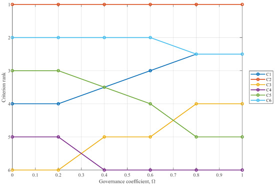
At $\alpha =0.5$, changing $\mathsf{\Omega }$ altered both weights and ranks (Table 11 and Figure 2). For example, the committee-only endpoint yielded $C_2>C_6>C_5>C_1>C_4>C_3$, whereas the superior-only endpoint yielded $C_2>C_1=C_6>C_3>C_5>C_4$. A tie between $C_1$ and $C_5$ occurred at $\mathsf{\Omega }=0.4$.

Table 11. UAV sensitivity to $\mathsf{\Omega }$ at $\alpha =0.5$.

$\mathsf{\Omega }$	${\mathit{C}}_1$	${\mathit{C}}_2$	${\mathit{C}}_3$	${\mathit{C}}_4$	${\mathit{C}}_5$	${\mathit{C}}_6$	${\mathbf{\Delta }}^{\ast }$
0.0	0.1331	0.3327	0.0798	0.0951	0.1597	0.1996	0.1924
0.2	0.1354	0.3250	0.0812	0.0928	0.1625	0.2031	0.1866
0.4	0.1504	0.2895	0.1015	0.0827	0.1504	0.2256	0.1691
0.6	0.1681	0.2881	0.1261	0.0720	0.1297	0.2161	0.1308
0.8	0.1877	0.2963	0.1407	0.0691	0.1185	0.1877	0.0751
1.0	0.1854	0.2927	0.1512	0.0683	0.1171	0.1854	0.0146

Figure 2. Criterion ranks across $\mathsf{\Omega }$ at $\alpha =0.5$.

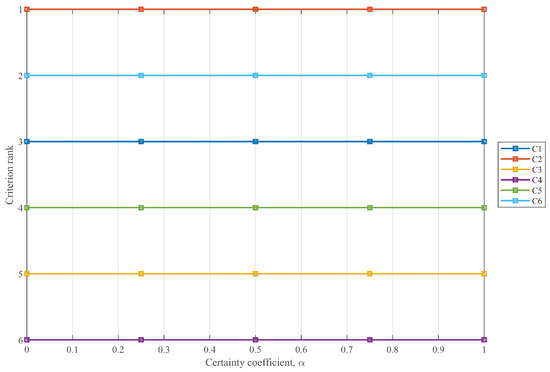
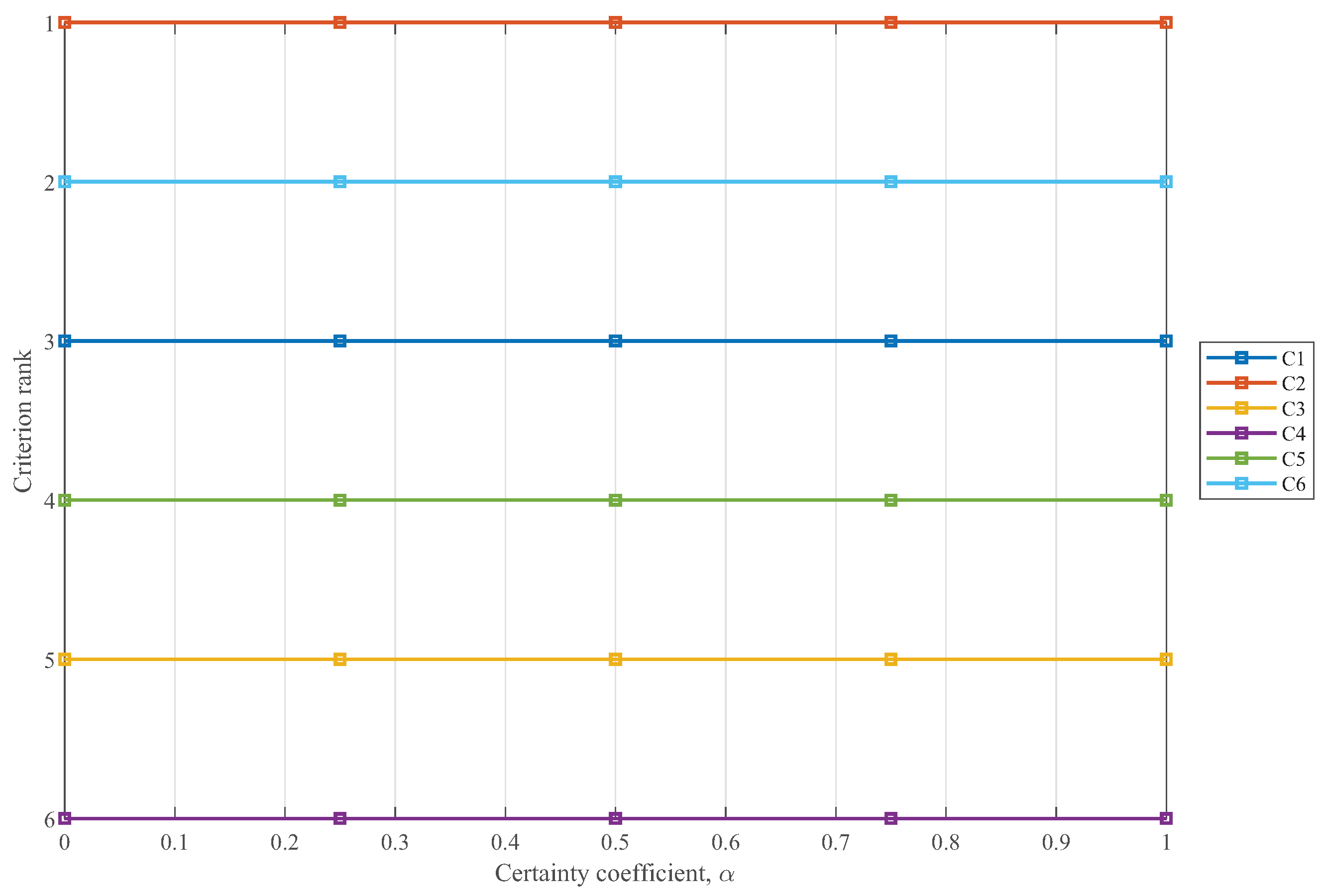
At $\mathsf{\Omega }=0.5$, the criterion vector and ranking remained constant over $\alpha \in [0,1]$. Transition roots were calculated from (32) and verified using neighboring LP optimality conditions. No valid breakpoint was detected (Figure 3). The expert weights and ${\Delta }^{\ast }$ still varied with $\alpha$, while the same LP extreme point remained optimal.

Figure 3. Criterion ranks across $\alpha$ at $\mathsf{\Omega }=0.5$; no ranking breakpoint was detected.

The same analytic check was applied at $\mathsf{\Omega }\in \{0,0.2,0.4,0.5,0.6,0.8,1\}$. One optimal-vertex breakpoint was found at $\mathsf{\Omega }=0.4$ and ${\alpha }^{\ast }\approx 0.0028$. The criterion vector changed from $(0.1556,0.2879,0.0934,0.0739,0.1556,0.2335)$ below the breakpoint to $(0.1504,0.2895,0.1015,0.0827,0.1504,0.2256)$ above it. Both vectors are optimal at ${\alpha }^{\ast }$ and have the order $C_2>C_6>C_1=C_5>C_3>C_4$; no valid $\alpha$ breakpoint was found at the other examined values of $\mathsf{\Omega }$.

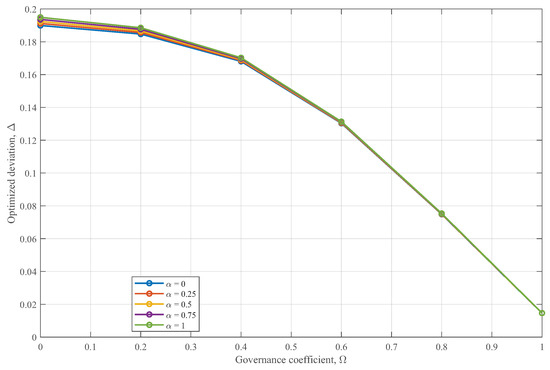
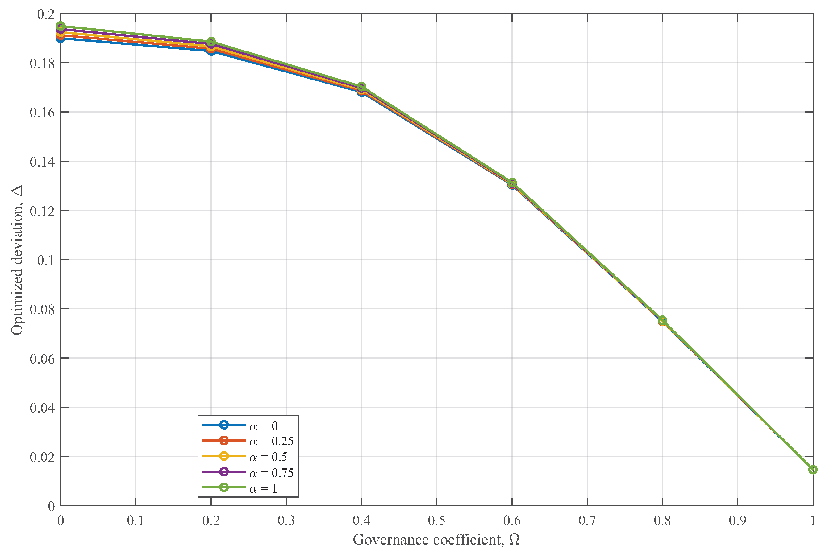
Differences in ${\Delta }^{\ast }$ summarize the weighted objective under each coefficient and are interpreted together with the weight and rank paths in Figure 4.

Figure 4. Optimized deviation across $\mathsf{\Omega }$ for selected values of $\alpha$.

For $n=6$ criteria and $l=4$ committee experts, the complete elicitation requires $(l+1)(2n-3)+(2l-3)=50$ unique comparisons. The main procedure solves $l+2=6$ LPs: one for prior expert weighting, four individual committee LPs, and one final superior–committee LP. Judgment agreement requires $O\left(l^{2}n\right)$ arithmetic operations. Table 12 reports a total measured runtime of 0.4689 s.

Table 12. LP dimensions and measured baseline runtime.

Component	LPs	Variables	Inequalities	Equalities	Runtime (s)
Prior committee weights	1	5	16	1	0.3135
Individual committee LIF-BWM models	4	7	24	1	0.1420
Final superior–committee LP	1	11	120	1	0.0134
Main procedure	6	–	–	–	0.4689

4. Discussion

LIFNs retain membership, non-membership, and indeterminacy during preference elicitation and in the entropy calculation. The optimization models use the scalar utility $U\left(\phi \right)$. Consequently, two LIFNs with the same utility generate identical BWM ratios even when their indeterminacy differs. The identical results from linear BWM and LIF-BWM confirm this computational relationship. Scalar utility determines the LP ratios, while the original LIFNs provide the certainty information.

The prior and judgment-derived expert weights also have distinct meanings. The prior component records the superior expert’s assessment of committee expertise. The judgment-derived component combines certainty with agreement derived from similarities among fitted weight vectors. The informed-dissent test shows how a strong prior assessment can preserve the influence of a coherent minority view. The inconsistency screen excludes contradictory inputs before aggregation, while the subgroup diagnostics reveal polarization that an average agreement score may conceal. These mechanisms allow agreement to be interpreted together with expertise, consistency, and subgroup structure.

Multiplicative integration requires joint support from the prior and judgment-derived components, whereas additive integration permits compensation. The ablation results preserved the criterion order under all five schemes, although the expert weights and objective values differed. The choice between the two forms therefore depends on whether compensation between the prior and judgment-derived components is acceptable.

The governance coefficient $\mathsf{\Omega }$ controls the objective coefficients of the superior and committee residual blocks. At $\mathsf{\Omega }=0.5$, the blocks receive equal coefficients, while their realized influence depends on their residual structures and committee weights. The two forms of superior influence operate at different levels: prior weights differentiate experts within the committee block, and $\mathsf{\Omega }$ allocates influence between the superior and committee blocks. The observed rank changes across $\mathsf{\Omega }$ show why its full sensitivity path should accompany the baseline result. The absence of an $\alpha$ breakpoint at $\mathsf{\Omega }=0.5$ follows from the active LP region identified for this case; the isolated breakpoint at $\mathsf{\Omega }=0.4$ changes the active vertex without changing the criterion order.

The superior–committee architecture can also support other fuzzy BWM environments. The representation-dependent modules are the comparison format, weight-derivation model, consistency measure, uncertainty measure, and similarity function. A triangular fuzzy implementation would replace the LIFNs with triangular comparisons and use the corresponding fuzzy optimization, defuzzification, and consistency procedures [11,12,38]. Interval-valued intuitionistic fuzzy, hesitant linguistic, Pythagorean fuzzy, and related environments can be incorporated when compatible modules are available. The two-stage role structure and the governance allocation remain unchanged at the architectural level.

Other pairwise-comparison methods can be adapted in the same manner. In an AHP implementation, reciprocal matrices replace the best-to-others and others-to-worst vectors. Eigenvector or logarithmic least-squares procedures provide the priority vectors, and the AHP consistency ratio screens the judgments. Prior committee weights can be elicited through a separate AHP matrix, after which certainty, agreement, and superior–committee integration follow the same two-stage logic. This adaptation increases the elicitation burden from $2n-3$ to $n(n-1)/2$ comparisons for each n-criterion assessment.

The controlled analyses quantify known-weight recovery under the specified perturbations and provide diagnostics for the constructed stress tests. Studies with domain experts can examine the practical selection of the governance parameters. Future work may also consider larger committees, comparisons with additional fuzzy BWM formulations, dynamic preference revision, and complete alternative-ranking applications.

5. Conclusions

This paper developed a systems-based superior–committee method for criteria weighting under linguistic intuitionistic fuzzy uncertainty. The formulation screens input consistency, calculates certainty from the $2n-3$ unique comparisons, and distinguishes prior expertise assessment from properties of the current judgments. The final LP preserves the superior and committee blocks and integrates them through an explicit governance coefficient.

The constructed UAV case produced the baseline order $C_2>C_6>C_1>C_5>C_3>C_4$. Controlled validation quantified recovery across 300 accepted instances, with a top-criterion recovery rate of 1.00 at all three perturbation levels. The harmonized comparison linked weight changes to the selected fuzzy representation, while ablation and stress tests clarified the effects of expert weighting, informed dissent, inconsistent inputs, and polarized subgroups. Sensitivity analysis further showed how $\mathsf{\Omega }$ changes the weights and why $\alpha$ can alter the objective without changing the active LP solution.

Future work may evaluate the method with empirical expert panels and extend it to larger decision groups, additional fuzzy BWM formulations, and alternative-ranking methods.

References

- Gao, F. Evaluating and selecting sustainable aviation fuel alternatives based on an interval-valued intuitionistic fuzzy decision-making approach. Aerosp. Sci. Technol. 2026, 177, 112912. [Google Scholar] [CrossRef] [Scilit]
- Liu, Y.; Eckert, C.M.; Earl, C. A review of fuzzy AHP methods for decision-making with subjective judgements. Expert Syst. Appl. 2020, 161, 113738. [Google Scholar] [CrossRef] [Scilit]
- Rezaei, J. Best-worst multi-criteria decision-making method. Omega 2015, 53, 49–57. [Google Scholar] [CrossRef] [Scilit]
- Rezaei, J. Best-worst multi-criteria decision-making method: Some properties and a linear model. Omega 2016, 64, 126–130. [Google Scholar] [CrossRef] [Scilit]
- Liang, F.; Brunelli, M.; Rezaei, J. Consistency issues in the best worst method: Measurements and thresholds. Omega 2020, 96, 102175. [Google Scholar] [CrossRef] [Scilit]
- Mi, X.; Tang, M.; Liao, H.; Shen, W.; Lev, B. The state-of-the-art survey on integrations and applications of the best worst method in decision making: Why, what, what for and what’s next? Omega 2019, 87, 205–225. [Google Scholar] [CrossRef] [Scilit]
- Tu, J.; Wu, Z.; Pedrycz, W. Priority ranking for the best-worst method. Inf. Sci. 2023, 635, 42–55. [Google Scholar] [CrossRef] [Scilit]
- Wu, Q.; Liu, X.; Zhou, L.; Qin, J.; Rezaei, J. An analytical framework for the best-worst method. Omega 2024, 123, 102974. [Google Scholar] [CrossRef] [Scilit]
- Ratandhara, H.M.; Kumar, M. An Analytical Framework for the Multiplicative Best–Worst Method. J. Multi-Criteria Decis. Anal. 2024, 31, e1840. [Google Scholar] [CrossRef] [Scilit]
- Peykani, P.; Emrouznejad, A.; Nouri, M. Best-worst multi-criteria decision-making method: A review of the literature. Socio-Econ. Plan. Sci. 2026, 104, 102345. [Google Scholar] [CrossRef] [Scilit]
- Guo, S.; Zhao, H. Fuzzy best-worst multi-criteria decision-making method and its applications. Knowl.-Based Syst. 2017, 121, 23–31. [Google Scholar] [CrossRef] [Scilit]
- Dong, J.; Wan, S.; Chen, S.M. Fuzzy best-worst method based on triangular fuzzy numbers for multi-criteria decision-making. Inf. Sci. 2021, 547, 1080–1104. [Google Scholar] [CrossRef] [Scilit]
- Wan, S.; Dong, J.; Chen, S.M. Fuzzy best-worst method based on generalized interval-valued trapezoidal fuzzy numbers for multi-criteria decision-making. Inf. Sci. 2021, 573, 493–518. [Google Scholar] [CrossRef] [Scilit]
- Wan, S.; Dong, J. A novel extension of best-worst method with intuitionistic fuzzy reference comparisons. IEEE Trans. Fuzzy Syst. 2022, 30, 1698–1711. [Google Scholar] [CrossRef] [Scilit]
- Seyfi-Shishavan, S.A.; Gundogdu, F.K.; Farrokhizadeh, E. An assessment of the banking industry performance based on Intuitionistic fuzzy Best-Worst Method and fuzzy inference system. Appl. Soft Comput. 2021, 113, 107990. [Google Scholar] [CrossRef] [Scilit]
- Cheng, X.; Chen, C. Decision Making with Intuitionistic Fuzzy Best-Worst Method. Expert Syst. Appl. 2024, 237, 121215. [Google Scholar] [CrossRef] [Scilit]
- Dong, J.Y.; Wan, S.P. Interval-valued intuitionistic fuzzy best-worst method with additive consistency. Expert Syst. Appl. 2024, 236, 121213. [Google Scholar] [CrossRef] [Scilit]
- Wan, S.P.; Dong, J.Y.; Chen, S.M. A novel intuitionistic fuzzy best-worst method for group decision making with intuitionistic fuzzy preference relations. Inf. Sci. 2024, 666, 120404. [Google Scholar] [CrossRef] [Scilit]
- Tavana, M.; Sorooshian, S.; Rezaei, H.; Mina, H. A novel fuzzy scenario-based stochastic general best-worst method. Expert Syst. Appl. 2024, 252, 124246. [Google Scholar] [CrossRef] [Scilit]
- Liao, H.; Mi, X.; Yu, Q.; Luo, L. Hospital performance evaluation by a hesitant fuzzy linguistic best worst method with inconsistency repairing. J. Clean. Prod. 2019, 232, 657–671. [Google Scholar] [CrossRef] [Scilit]
- Faizi, S.; Salabun, W.; Nawaz, S.; Rehman, A.u.; Watrobski, J. Best-Worst method and Hamacher aggregation operations for intuitionistic 2-tuple linguistic sets. Expert Syst. Appl. 2021, 181, 115088. [Google Scholar] [CrossRef] [Scilit]
- Zhang, R.; Xu, Z.; Gou, X. An integrated method for multi-criteria decision-making based on the best-worst method and Dempster-Shafer evidence theory under double hierarchy hesitant fuzzy linguistic environment. Appl. Intell. 2021, 51, 713–735. [Google Scholar] [CrossRef] [Scilit]
- Zhang, H. Linguistic intuitionistic fuzzy sets and application in MAGDM. J. Appl. Math. 2014, 2014, 432092. [Google Scholar] [CrossRef] [Scilit]
- Ou, Y.; Yi, L.; Zou, B.; Zheng, P. The linguistic intuitionistic fuzzy set TOPSIS method for linguistic multi-criteria decision makings. Int. J. Comput. Intell. Syst. 2018, 11, 120. [Google Scholar] [CrossRef] [Scilit]
- Meng, F.; Tang, J.; Fujita, H. Linguistic intuitionistic fuzzy preference relations and their application to multi-criteria decision making. Inf. Fusion 2019, 46, 77–90. [Google Scholar] [CrossRef] [Scilit]
- Garg, H.; Kumar, K. Linguistic interval-valued atanassov intuitionistic fuzzy sets and their applications to group decision making problems. IEEE Trans. Fuzzy Syst. 2019, 27, 2302–2311. [Google Scholar] [CrossRef] [Scilit]
- Akram, M.; Ilyas, F.; Garg, H. Multi-criteria group decision making based on ELECTRE I method in Pythagorean fuzzy information. Soft Comput. 2020, 24, 3425–3453. [Google Scholar] [CrossRef] [Scilit]
- Zhang, H.; Dai, Y. Consensus improvement model in group decision making with hesitant fuzzy linguistic term sets or hesitant fuzzy linguistic preference relations. Comput. Ind. Eng. 2023, 178, 109015. [Google Scholar] [CrossRef] [Scilit]
- Liu, P.; Dong, X.; Wang, P. Limited budget-based consensus model for large group decision making with hesitant fuzzy linguistic information. Appl. Soft Comput. 2023, 142, 110368. [Google Scholar] [CrossRef] [Scilit]
- Song, H.H.; Wang, Y.M.; Martinez, L. Enhancing group decision-making: Maximum consensus aggregation for fuzzy cross-efficiency under hesitant fuzzy linguistic information. Comput. Ind. Eng. 2024, 197, 110622. [Google Scholar] [CrossRef] [Scilit]
- You, X.; Hou, F.; Chiclana, F. A Reputation-Based Trust Evaluation Model in Group Decision-Making Framework. Inf. Fusion 2024, 103, 102082. [Google Scholar] [CrossRef] [Scilit]
- Yang, Y.; Zhang, K.; Lei, Z. A Consensus Reaching Process for Product Design Decision-Making by Integrating Intuitionistic Fuzzy Sets and Trust Network. Systems 2024, 12, 494. [Google Scholar] [CrossRef] [Scilit]
- Mou, Q.; Xu, Z.; Liao, H. An intuitionistic fuzzy multiplicative best-worst method for multi-criteria group decision making. Inf. Sci. 2016, 374, 224–239. [Google Scholar] [CrossRef] [Scilit]
- Martínez, L.; Herrera, F. A 2-tuple fuzzy linguistic representation model for computing with words. IEEE Trans. Fuzzy Syst. 2000, 8, 746–752. [Google Scholar] [CrossRef] [Scilit]
- Atanassov, K.T. Intuitionistic fuzzy sets. Fuzzy Sets Syst. 1986, 20, 87–96. [Google Scholar] [CrossRef] [Scilit]
- Li, Z.; Liu, P.; Qin, X. An extended VIKOR method for decision making problem with linguistic intuitionistic fuzzy numbers based on some new operational laws and entropy. J. Intell. Fuzzy Syst. 2017, 33, 1919–1931. [Google Scholar] [CrossRef] [Scilit]
- Gao, F. An integrated multi criteria decision making method using dual hesitant fuzzy sets with application for unmanned aerial vehicle selection. Sci. Rep. 2025, 15, 12637. [Google Scholar] [CrossRef] [Scilit] [PubMed]
- Komatina, N.; Marinković, D.; Simić, V.; Banduka, N.; Nešović, A. A Hybrid Fuzzy Decision-Making Algorithm for Prioritization of the 8D Problem-Solving Methodology Using FBWM and FSREM. Algorithms 2026, 19, 510. [Google Scholar] [CrossRef] [Scilit]
Disclaimer/Publisher’s Note: The statements, opinions and data contained in all publications are solely those of the individual author(s) and contributor(s) and not of MDPI and/or the editor(s). MDPI and/or the editor(s) disclaim responsibility for any injury to people or property resulting from any ideas, methods, instructions or products referred to in the content. |
© 2026 by the authors. Licensee MDPI, Basel, Switzerland. This article is an open access article distributed under the terms and conditions of the Creative Commons Attribution (CC BY) license.