


Highlights
Please indicate how your work links to systems science via your contributions to systems practice, theory, and/or methodology.
- This study conceptualizes emergency procurement as a system-level coopetition mechanism in complex supply chains where critical inputs are not readily interchangeable.
- It develops a game-theoretic model linking upstream disruption risk, technology conversion costs, downstream Cournot competition, firm profits, consumer surplus, and social welfare.
What are the main findings and/or the implications of the main findings?
- Market potential, relative cost advantage, and conversion costs jointly determine whether competing NEV manufacturers enter competition-only, cooperation-only, or coopetition regimes.
- Emergency procurement changes pre-disruption quantity decisions and restores supply after disruptions, while its effects on consumer surplus and social welfare depend on market structure, technology conversion costs, and product substitutability.
Abstract
Amid increasing upstream raw-material disruptions and battery supply uncertainty, NEV manufacturers may obtain emergency supply from vertically integrated competitors after a disruption, but must incur technology conversion costs. We develop a differentiated Cournot duopoly model with an outsourcing manufacturer and an integrated manufacturer to compare equilibrium, profit, and welfare outcomes with and without emergency procurement cooperation. The results show that cooperation has a clear feasibility boundary jointly determined by market potential, relative costs, and conversion costs, giving rise to competition-only, cooperation-only, and coopetition regimes. The cooperation option reshapes pre-disruption quantity decisions: the outsourcing manufacturer increases regular procurement, while the integrated manufacturer reduces its own-brand output by a larger amount. Within the cooperation region, higher conversion costs continuously reduce the outsourcing manufacturer’s profit, whereas the integrated manufacturer’s profit can be U-shaped. Greater product substitutability makes cooperation more fragile and widens the divergence between private profit incentives and supply-chain resilience. Consumer surplus and social welfare may also move in different directions, depending on the outsourcing manufacturer’s benchmark market share and conversion cost. A Nash-bargaining extension confirms the robustness of the activation condition and pre-disruption quantity-adjustment mechanism, while reducing emergency markups and improving consumer surplus.
1. Introduction
In recent years, natural disasters, geopolitical conflicts, trade frictions, and labor disputes have continued to increase the risk of global supply chain disruptions. To strengthen supply security, firms often adjust their supplier portfolios and increase vertical integration to reduce their exposure to such risks [1,2]. New energy vehicle (NEV) supply chains are particularly vulnerable to these disruptions. Different power-battery technologies rely on distinct combinations of critical minerals, such as lithium, nickel, and cobalt, and involve different supply network structures, resulting in varying levels of disruption vulnerability [3]. Meanwhile, growing pressure to reduce global carbon emissions is accelerating industrial decarbonization, resource recycling, and the low-carbon transition of the transportation sector [4,5]. The resulting expansion in demand for NEVs and power batteries further increases automakers’ dependence on geographically concentrated critical minerals and cross-border battery supply networks. Against the combined backdrop of low-carbon transition and supply uncertainty, how to allocate capacity effectively and restore the supply of critical components promptly after upstream disruptions has become an important operational issue in NEV supply chain management.
To enhance supply-chain resilience, NEV manufacturers have increasingly strengthened their control over critical component supply by securing key mineral resources, taking equity stakes in upstream firms, signing long-term supply agreements, and building safety stock. Compared with manufacturers that rely primarily on external sourcing, firms with in-house battery production capabilities or a higher degree of vertical integration generally have stronger supply assurance. Meanwhile, the global power-battery market is highly concentrated. In 2023, CATL, BYD, and LG Energy Solution together accounted for 65.6% of the global market, while the top ten suppliers collectively held a 93.8% share. Such market concentration weakens NEV manufacturers’ control over the power-battery supply chain [6]. Therefore, for traditional automakers transitioning from internal-combustion vehicles to NEVs, as well as light-asset manufacturers that focus on vehicle integration and brand management while relying largely on external sourcing, restoring the supply of critical components promptly after upstream disruptions remains an important operational challenge.
Because critical resources and production capacity in the NEV supply chain are highly concentrated, upstream disruptions often leave manufacturers with limited substitution options and slow recovery. These risks become more pronounced when disruption uncertainty is high and multiple manufacturers compete simultaneously for the same critical components in an increasingly homogeneous market. To manage such risks, manufacturers typically combine pre-disruption and post-disruption strategies. Pre-disruption measures, such as multi-sourcing and safety stock, reduce exposure to supply interruptions, whereas post-disruption responses, including emergency procurement, substitute sourcing, and hybrid strategies, help alleviate supply shortfalls after a disruption occurs [7,8,9]. In practice, NEV manufacturers are diversifying their access to critical components through cross-firm battery supply, joint production, and technology licensing. For example, Tesla has procured Blade Batteries from BYD, while Toyota and Panasonic established a joint venture for automotive battery production [6,10,11]. Such arrangements provide firms with alternative sources of battery supply when their regular external supply is constrained.
However, cooperation with competitors also entails important operational and strategic trade-offs. Compared with traditional automotive manufacturing, where mature powertrain technologies and more standardized components allow greater sourcing flexibility, NEV manufacturers rely on critical components that are high in value, technologically dynamic, and subject to stringent storage and compliance requirements. Integrating externally sourced technologies therefore often requires substantial adaptation, coordination, testing, validation, and other technology conversion activities. In addition, sharing platforms or critical components may reduce product differentiation, compress margins, and intensify downstream competition. These concerns are particularly relevant in the NEV industry, where core technologies and critical supply capacity are concentrated among a limited number of leading firms. An outsourcing manufacturer facing a disruption may therefore have few feasible alternatives and may need to procure emergency supply from a competing manufacturer. Such cooperation involves a clear trade-off: it can restore access to critical components but it also imposes adaptation and conversion costs and may strengthen downstream competitive pressure. Hence, the value of emergency procurement depends not only on the availability of alternative supply but also on the extent to which firms can reduce conversion frictions while preserving product differentiation.
These observations motivate three research questions. (1) Under what market-potential, cost, and technical-feasibility conditions does emergency procurement from a competitor arise, and when do the two manufacturers operate under competition-only, cooperation-only, or coopetition regimes? (2) How does the availability of emergency procurement reshape pre-disruption quantity decisions, post-disruption supply recovery, and the manufacturers’ profits as technology conversion cost and product substitutability vary? (3) Under what conditions does emergency procurement improve consumer surplus and social welfare, and when do these two welfare effects diverge?
To address these questions, we develop a supply chain coopetition model based on supply risk management and differentiated Cournot competition. The model features an outsourcing manufacturer exposed to upstream supply disruption risk and an integrated manufacturer. We first derive the benchmark equilibrium without cooperation. We then introduce an emergency procurement option under which the integrated manufacturer provides emergency supply following its rival’s upstream disruption, while the outsourcing manufacturer incurs a technology conversion cost. We use the resulting equilibria to examine how emergency procurement cooperation affects quantity decisions, firm profits, consumer surplus, and social welfare. Finally, we introduce asymmetric generalized Nash bargaining as an alternative emergency pricing mechanism to assess the robustness of the main findings.
Although the model is developed in the context of NEV battery-cell supply, it captures a broader systems mechanism in which emergency replenishment is constrained by critical inputs that are not readily interchangeable. When components are closely embedded in product architectures, technical interfaces, production processes, and qualification procedures, replacing a disrupted source requires adaptation, validation, and coordination across interdependent firms. Emergency procurement therefore represents a system-level coopetition problem that links upstream supply recovery, technology conversion, downstream competition, and welfare outcomes.
The main contributions are threefold. First, we introduce a decision perspective in which a manufacturer uses emergency procurement from a competitor to cope with upstream supply disruptions. By systematically comparing competition-only, cooperation-only, and coopetition equilibria, we show how market potential, relative costs, and technology conversion costs jointly determine the boundary of emergency procurement cooperation and the resulting coopetition structure. This extends the analysis of coopetition to supply disruption settings. Second, we incorporate technology conversion costs into the coopetition decision framework and reveal the pre-disruption quantity-adjustment mechanism induced by emergency procurement cooperation. Cooperation increases the outsourcing manufacturer’s regular procurement quantity but leads the integrated manufacturer to reduce its own-brand output by a larger amount. As a result, total market supply contracts in the no-disruption state but is restored in the disruption state. Technology conversion costs also have asymmetric effects on the expected profits of the two manufacturers. Third, we characterize the welfare boundaries of emergency cooperation. Consumer surplus and social welfare do not necessarily improve simultaneously; their improvement conditions depend on the market structure and technology conversion cost. Moreover, greater product substitutability makes the two welfare effects more likely to diverge. These results provide more targeted theoretical implications for firms’ coopetition decisions and related policy design.
The remainder of this paper is organized as follows. Section 2 reviews the literature on supply disruption management, supply chain coopetition, and horizontal cooperation in NEV supply chains. Section 3 presents the differentiated duopoly model involving an outsourcing manufacturer and a vertically integrated manufacturer. Section 4 derives the no-cooperation benchmark. Section 5 analyzes equilibrium decisions under the emergency procurement option and examines its effects on market structure, quantity decisions, firm profits, consumer surplus, and social welfare. Section 6 extends the analysis by introducing asymmetric generalized Nash bargaining as an alternative emergency pricing mechanism and examines the robustness of the main results. Section 7 concludes the paper.
2. Literature Review
This study is closely related to three streams of literature: supply disruption management, supply chain coopetition between competitors, and cooperation in NEV battery supply chains. When manufacturers face upstream supply disruptions, timely access to alternative supply directly affects production recovery and the resulting profit losses. Existing research has examined two broad approaches: pre-disruption mitigation and post-disruption response. Before a disruption occurs, firms typically reduce their risk exposure through safety stock, multi-sourcing, and resilience investments. After a disruption or delivery shortfall, they may reallocate orders or use emergency procurement to fill the resulting supply gap [7,12,13,14,15,16,17]. Extending this literature, some studies incorporate suppliers’ strategic pricing and show that although backup supply can facilitate production recovery, it may also alter competition among suppliers and therefore does not necessarily benefit the buyer or the supply chain as a whole [18,19]. When competition exists across supply chains, supply reliability can further affect manufacturers’ quantity decisions and their choice of supply chain structure [20]. Singla et al. further examine how competing firms reserve limited backup resources ex ante and procure them ex post, highlighting both short-term sales losses and persistent shifts in market share following supply disruptions [21]. In most of this literature, however, backup supply is provided by independent external suppliers or shared supply markets that do not directly compete in the final-product market. Even when the purchasing manufacturers compete with one another, relatively little attention has been paid to settings in which one downstream competitor directly supplies critical components to a disrupted rival. Thus, when backup capacity is controlled by a competing manufacturer, how emergency procurement cooperation jointly affects supply recovery and downstream market competition remains underexplored.
When critical components are supplied by a competitor in the final market, post-disruption emergency procurement has both cooperative and competitive features. The supplying firm can earn additional revenue from the emergency transaction, but restoring its rival’s production also intensifies downstream competition and erodes profits from its own products. Emergency supply between competing manufacturers therefore involves a trade-off between supply-side gains and downstream competitive losses. Research on coopetition under normal operating conditions has shown that production cost differences, product substitutability, bargaining power, and decision timing can affect component wholesaling, production outsourcing, and the choice of cooperation mode between competitors [22,23]. Related studies have further examined dual sourcing when a competitive supplier coexists with an unreliable non-competing supplier, as well as information leakage and dual-sourcing decisions when a vertically integrated firm supplies an outsourcing rival in the final market [24,25]. The former focuses on order allocation before supply uncertainty is realized, whereas the latter examines supply relationships under normal operating conditions. Neither treat an actual upstream disruption as the direct trigger for supply from a competitor. Research on capacity sharing and horizontal procurement, by contrast, mainly considers resource reallocation under demand uncertainty, capacity constraints, or production cost asymmetry [26,27,28], with the primary objective of mitigating supply–demand mismatches or improving capacity utilization. Building on this literature, we consider a setting in which, after an upstream supply disruption occurs, a vertically integrated manufacturer provides emergency supply to an outsourcing competitor. The integrated manufacturer first sets the emergency wholesale price, after which the outsourcing manufacturer determines its emergency procurement quantity. The two firms then compete in the same downstream market. Whether emergency procurement occurs, and at what scale, depends on whether the supplying manufacturer’s gains from the emergency transaction are sufficient to offset the profit loss caused by intensified downstream competition.
The NEV supply chain provides a particularly relevant industry setting for the above problem. One stream of research focuses on horizontal coopetition among NEV manufacturers in the supply of power batteries. Zhu et al. examine whether a vertically integrated automaker with in-house battery production supplies batteries to a downstream competitor and show how external procurement costs affect battery capacity allocation, firm profits, and social welfare [10]. Zhang and Wang further consider two manufacturers that can both produce batteries in-house but differ in battery performance, and show that battery supply cooperation between an incumbent and an emerging manufacturer depends on the latter’s cost conditions and government subsidies [29]. Another stream compares alternative cooperation modes, including battery wholesaling, patent licensing, and joint production, and finds that product substitutability, technological innovation, government subsidies, and information about battery quality can affect the choice of cooperation mode and the resulting profit allocation [6,11]. Research on closed-loop supply chains further extends cooperation to battery-recycling process innovation, showing that the viability of joint investment depends on innovation efficiency and the distribution of power within the supply chain [30]. Together, these studies show that cooperation among NEV manufacturers is highly conditional. However, existing research mainly considers supply agreements, licensing, joint ventures, or collaborative innovation arrangements established under normal operating conditions, while paying relatively limited attention to the compatibility of critical components in horizontal cooperation. This issue becomes particularly important for emergency procurement after a disruption. In automotive supply chains, application-engineering investments in critical components create relationship-specific knowledge tied to particular vehicle platforms and supplier relationships, so switching suppliers on short notice requires renewed coordination in design, production, and validation [31]. Such cross-firm coordination and production-conversion costs become more pronounced as product complexity and component coupling increase [32]. Power batteries illustrate this problem clearly: the design of battery cells, modules, and packs remains insufficiently standardized, and alternative configurations are often not directly interchangeable [33]. Consequently, a competitor’s available battery capacity cannot necessarily be converted immediately into usable supply for a disrupted manufacturer. Cross-platform adoption may still require interface adaptation, system integration, testing, and validation.
To capture these operational frictions, we summarize the required adaptation efforts as a technology conversion cost and incorporate it into the post-disruption emergency procurement decision. The model jointly considers upstream supply disruption, the competitor’s emergency pricing decision, and the disrupted manufacturer’s procurement decision. This framework allows us to characterize the conditions under which emergency supply between competitors arises and to examine how technology conversion costs differentially affect firm profits, consumer surplus, and social welfare.
3. Model Setup
We consider two competing NEV manufacturers, and . , the outsourcing manufacturer, relies primarily on external sourcing for critical components, particularly batteries. Representative firms include NIO, XPeng, Li Auto, and Xiaomi. Such manufacturers typically have weaker control over critical component supply and may therefore face greater exposure to upstream disruptions and supplier-switching costs. In the NEV industry, battery cells are highly platform-specific and closely integrated with vehicle design, while supplier changes often require lengthy certification and validation procedures. Consequently, switching battery suppliers on short notice after a disruption can incur substantial technology conversion costs, including those associated with battery-pack interface adaptation, thermal management, battery management system calibration, validation testing, and production-line tooling adjustments.
In contrast, , the vertically integrated manufacturer, (hereafter, the integrated manufacturer), has greater in-house control over critical components and production capacity. Representative firms include BYD, Tesla, and Great Wall Motor. Such manufacturers typically integrate the development and production of major modules, including battery cells, battery packs, electric powertrains, domain controllers, vehicle assembly, and software. In particular, in-house battery-cell production can improve cost control and supply assurance. Because the integrated manufacturer has greater control over critical capacity and core technologies, it is less exposed to upstream rationing and supply-priority downgrades and therefore faces lower disruption risk. Cross-firm supply relationships are also observed in practice. For example, BYD supplies batteries for Toyota’s bZ3, while Tesla has supplied battery packs or motors to Daimler and electric drive systems for the Toyota RAV4 EV. Accordingly, when experiences an upstream disruption, it may seek emergency supply from . A related example is General Motors’ reported use of CATL battery packs as a transitional solution to address a short-term shortage of low-cost LFP batteries. Table 1 summarizes the notation used throughout the model.
Table 1.
List of symbols and definitions.
The outsourcing manufacturer procures its critical component from an external supplier and is therefore exposed to upstream supply disruption risk. Without loss of generality, we assume that producing one vehicle requires one unit of battery cells, purchased at a unit cost () [30]. Before the supply state is realized, chooses a pre-disruption order quantity , which represents its regular procurement quantity when no disruption occurs. The upstream supplier may be disrupted by natural disasters, political instability, labor strikes, technical failures, supplier bankruptcy, or other unexpected events [9]. We represent its delivery outcome by a Bernoulli random variable , and, unless otherwise stated, expectations are taken with respect to . Specifically, denotes supplier reliability, so the realized delivery quantity is . We further assume a pay-for-delivery arrangement, under which pays only for the quantity actually delivered, yielding a procurement payment of [34].
In contrast, the integrated manufacturer has greater control over battery supply through long-term supply agreements, equity partnerships, and in-house production. To isolate the focal mechanism, we follow models that distinguish an unreliable regular source from a reliable backup or expedited source [7,15,18,19] and assume that ’s internal battery supply remains available when is disrupted. The focal shock is supplier-specific rather than industry-wide: does not source battery cells from and has greater control over critical inputs through vertical integration [2]. This assumption isolates competitor-based emergency supply and does not imply that integrated manufacturers are immune to all supply disruptions. Accordingly, ’s in-house battery-cell production is not exposed to the focal supplier-specific disruption and incurs a unit production cost (). Manufacturer chooses the battery-cell production quantity for its own branded vehicles. When the cooperation option is unavailable, the two manufacturers simultaneously choose their respective regular procurement and production quantities.
With the cooperation option available, the supply chain structure is shown in Figure 1. Because NEV production is typically planned well in advance, production lead times are generally 6–12 months, compared with 2–6 months for internal-combustion vehicles. Given these long lead times, when the upstream supplier is disrupted (), the outsourcing manufacturer can procure battery cells from its competitor, the integrated manufacturer , as an emergency supply to complete production. Accordingly, when no disruption occurs (), ’s realized output is ; when a disruption occurs (), its realized output is . Thus, ’s realized output across the two supply states can be written as . The integrated manufacturer’s realized output is .
Figure 1.
Supply chain structure.
The decision sequence under the cooperation option is illustrated in Figure 2. Before the supply state is realized, the two manufacturers simultaneously choose and . This stage is modeled as differentiated Cournot competition, consistent with quantity-competition and coopetition models under supply uncertainty [20,22,23]. After the supply state is realized, if is disrupted, first sets the emergency wholesale price , and then chooses ; otherwise, the emergency procurement stage is not activated. The resulting sequential emergency transaction constitutes a Stackelberg price–quantity subgame. This separation between initial decisions and emergency sourcing after supply information becomes available is consistent with contingent-sourcing models [19].
Figure 2.
Decision sequence with the cooperation option.
We model emergency procurement between competitors as a short-term, disruption-contingent arrangement rather than routine procurement under a long-term agreement. Following a sudden disruption, the outsourcing manufacturer may face delivery failures, production stoppages, and potential market-share losses, while alternative sources are often difficult to secure within a short time. Because the integrated manufacturer controls critical component supply and has greater flexibility in capacity allocation, it is assumed to have greater bargaining power in the emergency procurement stage. We therefore adopt post-disruption pricing to characterize price formation in this stage. When supplier is disrupted, the integrated manufacturer acts as the leader and sets the emergency wholesale price for battery cells. The outsourcing manufacturer then chooses the emergency procurement quantity . Consistent with the emergency nature of this arrangement, we assume that other regular suppliers cannot provide additional supply within the short emergency window, whereas emergency supply from is reliable. Thus, once an agreement is reached, the emergency procurement quantity is delivered as scheduled.
In addition to regular procurement and component production costs, we introduce a per-unit technology conversion cost . We define narrowly as the technical adaptation and supplier-switching cost incurred when the outsourcing manufacturer adopts batteries supplied by the integrated manufacturer . Such costs arise because switching suppliers for complex automotive components requires supplier-specific engineering and coordination, while differences in battery-cell, module, and pack designs may further increase the required adaptation effort [31,32,33]. Accordingly, when an upstream disruption forces to switch battery sources, it may need to undertake engineering activities required for mass production, including functional and safety recertification, wiring-harness and interface adaptation, and production-line tooling adjustments. The associated expenditure depends on the compatibility between the emergency-supplied battery cells and ’s vehicle platform and production system. All other costs are normalized to zero [35,36].
The inverse demand functions faced by manufacturers and are given by:
where denotes market potential, that is, the intercept of the inverse demand function, and and denote the realized market quantities of and , respectively. Parameters and B capture the own- and cross-quantity effects in inverse demand, with (). Thus, the two products are imperfect substitutes, and each manufacturer’s own quantity has a stronger effect on its price than the rival’s quantity. For a given , a larger indicates greater product substitutability [37]. We impose the following assumption to ensure economically meaningful outcomes.
Assumption 1.
, , and , where (). These conditions require market potential to exceed the relevant marginal supply costs. In particular, when a disruption occurs, represents the minimum per-unit cost associated with emergency supply to , consisting of the integrated manufacturer’s production cost and the technology conversion cost. The assumption rules out trivial parameter regions in which supplying the market is not economically viable [20,22,23].
4. Decision Analysis Under the No-Cooperation Benchmark
To examine how the cooperation option affects the two manufacturers’ decisions, we first analyze the no-cooperation benchmark. Specifically, the integrated manufacturer does not provide emergency supply, and the two manufacturers simultaneously choose their production quantities. In this setting, chooses only its regular pre-disruption procurement quantity , regardless of whether a disruption subsequently occurs. To distinguish this benchmark from subsequent analyses, we use the superscript to denote no cooperation; the same notation is used hereafter.
Given ’s production quantity , manufacturer chooses its regular procurement quantity to maximize its expected profit:
Because the cooperation option is unavailable, cannot obtain emergency supply from ; hence, its realized market quantity is . Here, represents ’s revenue, and represents its regular procurement cost.
Given ’s realized quantity , manufacturer chooses to maximize its expected profit:
In this expression, denotes ’s revenue, while represents its production cost. Solving the above problems yields Proposition 1.
Proposition 1.
Under the non-negativity constraints, define the two market-potential thresholds as , If , the equilibrium quantities under the no-cooperation benchmark are . (All proofs are provided in the Appendix A.)
Proposition 1 shows that, under the non-negativity constraints on quantities, two market-potential thresholds, and , can be defined. If and only if , both the outsourcing manufacturer and the integrated manufacturer remain active under the no-cooperation benchmark, with equilibrium quantities and , respectively. The thresholds and represent the minimum market-potential levels required for the two manufacturers to coexist. Moreover, the market potential required for coexistence increases with product substitutability. This suggests that, in submarkets with limited product differentiation and highly homogeneous core components, manufacturers with lower costs and more stable supply and capacity are better positioned to remain viable over the long run. Based on Proposition 1, we obtain the following corollary.
Corollary 1.
(i) When , . If , then and .
(ii) When , . If , then and .
Since , the ordering of the two thresholds is determined by the manufacturers’ relative costs. When the integrated manufacturer has a cost advantage (), . In this case, when market potential is low (), the outsourcing manufacturer exits the market because it cannot sustain a positive equilibrium quantity, leaving as the sole active producer with output . The result is symmetric when has a cost advantage. Moreover, increases with and decreases with , whereas increases with and decreases with . The negative effect of on becomes stronger as upstream reliability increases. Therefore, a greater cost reduction lowers the market-potential threshold required for a manufacturer to reach the coexistence region. When market demand is relatively low, the cost-disadvantaged manufacturer is consequently more likely to exit the market.
Corollary 2.
(i) , and .
(ii) , , , .
(iii) If , then ; if , then .
Corollary 2 shows that, provided , an increase in market potential v raises the equilibrium quantities of both manufacturers. However, . Thus, when the outsourcing manufacturer is exposed to upstream disruption risk, the integrated manufacturer responds more strongly to market expansion. Moreover, as the reliability of the outsourcing manufacturer’s upstream supplier increases, the difference in the two manufacturers’ responses to market potential gradually narrows. In the NEV market, sustained policy support, continued improvements in charging infrastructure, and rapid technological advances can stimulate market demand. Under such demand expansion, the integrated manufacturer tends to increase its output more strongly than the outsourcing manufacturer. By contrast, high upstream volatility or strong product substitutability can further weaken the competitive position of an outsourcing manufacturer exposed to supply disruption risk.
Comparative statics with respect to the cost parameters further show that each manufacturer’s equilibrium quantity decreases with its own cost and increases as its rival’s cost rises. Accordingly, the outsourcing manufacturer can reduce its exposure to supply disruptions by improving upstream supply reliability while controlling its production costs through bulk procurement and process improvements. The integrated manufacturer, in turn, can further reduce its unit cost through learning effects and capacity investment. In addition, a cost-disadvantaged manufacturer can use product differentiation to reduce the competitive pressure it faces and lower the market-potential requirement for market coexistence.
5. Decision Analysis with a Cooperation Option
5.1. Equilibrium Decisions
In the NEV battery supply chain, emergency cooperation between competitors has been observed in practice. For example, after Tesla’s in-house battery manufacturing efforts encountered setbacks in 2022, it procured LFP Blade Batteries from BYD; in 2024, NIO signed a battery supply agreement with BYD for its new brand, “Onvo.” Motivated by these industry developments, this section analyzes the equilibrium decisions when the integrated manufacturer and the outsourcing manufacturer have the option to cooperate.
When the external supplier of experiences a supply disruption, can provide the battery cells required for production to at a wholesale price . Unlike under the no-cooperation benchmark, determines not only its regular pre-disruption procurement quantity but also the emergency procurement quantity in the disruption state. Meanwhile, chooses its production quantity and the emergency wholesale price .
To characterize the equilibrium under the cooperation option, we solve the dynamic game by backward induction. Specifically, given , , and , we first determine ’s optimal emergency procurement quantity in the disruption state. If , the external supplier is not disrupted, so ; if , the external supplier is disrupted, and solves the following optimization problem:
Next, we consider the integrated manufacturer’s wholesale-price decision. Given ’s regular procurement quantity and ’s production quantity , if , the external supplier is not disrupted, emergency procurement is not activated, and does not need to set a wholesale price . If , the two manufacturers enter the emergency procurement subgame, in which chooses the wholesale price (. The corresponding decision problem is given by Equation (6).
We then characterize ’s regular procurement decision and ’s production decision . Given ’s production quantity , chooses to maximize its expected profit, as shown in Equation (7).
Given ’s regular procurement quantity , chooses to maximize its expected profit, as shown in Equation (8).
Solving the four optimization problems sequentially yields the following result.
Proposition 2.
The non-negativity constraints on the equilibrium quantities yield the following downstream market-participation thresholds for the outsourcing manufacturer and the integrated manufacturer, respectively: and . When market potential satisfies and the feasibility condition for positive emergency procurement after a disruption, , also holds, both manufacturers remain active in the downstream market. Their pre-disruption equilibrium decisions are , . After the supply state is realized, the equilibrium emergency procurement quantity and wholesale price are , . (All equilibrium expressions are reported in detail in Appendix A.)
Proposition 2 shows that, because the outsourcing manufacturer is exposed to upstream supply disruption risk whereas the integrated manufacturer is not, one might expect to exploit its supply advantage by prioritizing its own downstream market rather than providing emergency supply to a competing manufacturer after a disruption. The equilibrium results, however, show that this intuition does not hold when market potential is sufficiently high, , and positive emergency procurement is feasible . Even though and compete horizontally in the downstream market, emergency procurement cooperation still occurs. For , allowing emergency procurement enables it to convert part of its available capacity into wholesale profit at the equilibrium wholesale price , creating an additional source of revenue beyond its downstream retail business. For , emergency procurement mitigates the sales losses caused by upstream supply disruptions and helps it remain active in the market despite the absence of safety stock.
Corollary 3.
(i) When , . If , the outsourcing manufacturer exits the downstream market and the integrated manufacturer becomes the sole active producer. In this case, , , , and is undefined.
(ii) When and , . If , the integrated manufacturer exits the downstream market and instead becomes an upstream backup supplier that offers emergency supply to the outsourcing manufacturer. In this case, , , and .
When has a cost advantage (), in the low-market-potential region (), cannot sustain a positive equilibrium quantity and therefore exits the downstream market. The integrated manufacturer then serves the market alone with output . In this region, the two manufacturers compete without engaging in emergency procurement cooperation. By contrast, when has a cost advantage (), the outcome differs from that under the no-cooperation benchmark in Corollary 1. Even when market potential is relatively low, (), the integrated manufacturer does not leave the supply chain because of its cost disadvantage. Instead, it exits the downstream market and becomes an upstream backup supplier to . The two manufacturers no longer compete for downstream market share in this region. When a disruption occurs (), they engage in emergency procurement cooperation with . Thus, their relationship is characterized by cooperation without downstream competition.
5.2. Coopetition Relationships
This section examines the coopetition relationship between the two competing manufacturers, and , when a cooperation option with the rival is available. Based on Proposition 2, we obtain Proposition 3.
Proposition 3.
When the cooperation option is available, the competition–cooperation relationship between the outsourcing manufacturer and the vertically integrated manufacturer is characterized as follows:
(i) When and , we have , , and . In this region, competition and cooperation coexist between the two manufacturers.
(ii) When , If , we have , , and . The two manufacturers compete without cooperation: exits the downstream market, while becomes the sole active producer.
(iii) When and , if , we have , , and . The two manufacturers cooperate without downstream competition: becomes the sole active downstream producer, while becomes a backup supplier to .
Proposition 3 provides an intuitive characterization of three interaction patterns between the outsourcing manufacturer and the integrated manufacturer as market potential and relative costs vary. Depending on these conditions, the two firms may exhibit coopetition, cooperation without downstream competition, or competition without cooperation. When market potential is sufficiently high, both manufacturers remain active in the downstream market regardless of which firm has the cost advantage, while also engaging in emergency procurement cooperation. Strong market demand allows both firms to maintain positive market shares, and emergency procurement cooperation enables them to share disruption risk and capture additional gains from serving a high-demand market.
When has a cost advantage and market potential is relatively low, earns only limited profit from continuing to compete in the downstream market under its own brand and also faces direct competition from the lower-cost . In this case, exits the downstream market and instead supplies batteries upstream, earning wholesale profit without engaging in retail competition. By contrast, when has a cost advantage () and market potential is low, exits the market due to its disadvantages in both cost and supply reliability. Under these conditions, even when the cooperation option is available, emergency procurement cannot generate sufficient profit for to cover its production cost and the additional technology conversion cost.
5.3. Effect of the Cooperation Option on Equilibrium Outcomes
Corollary 4.
(i) If and , then .
(ii) If and , then .
As shown in Figure 3, Regions II and III correspond to the parameter ranges in which is the sole active producer under the no-cooperation benchmark, whereas Region IV corresponds to the range in which is the sole active producer. When has a cost advantage, introducing the cooperation option reduces its sole-producer region relative to the no-cooperation benchmark, with the reduction occurring in Region II. When the technology conversion cost is sufficiently low, (), emergency procurement improves ’s profitability under supply disruptions, allowing it to remain active in the downstream market. When has a cost advantage, introducing the cooperation option expands its sole-producer region when the technology conversion cost is low, (), with the expansion corresponding to Region I. The intuition is that, without the cooperation option, exits the downstream market when it is cost-disadvantaged. With the cooperation option, no longer competes downstream under its own brand but instead becomes an upstream backup supplier to , thereby mitigating ’s exposure to upstream disruption risk. As a result, can earn wholesale profit from emergency supply in the disruption state, while the interaction between the two manufacturers shifts toward cooperation without downstream competition.
Figure 3.
Effect of the cooperation option on the competitive outcome.
Corollary 4 further shows that the cooperation option not only shifts the boundaries of the sole-producer regions but also changes competitive intensity and the form of coopetition under different cost configurations. When the technology conversion cost is low, cooperation with a rival weakens downstream competition between the two manufacturers.
Corollary 5.
(i) When and , , . When and , , .
(ii) For the two cost configurations, the conversion-cost thresholds satisfy and , and, in proportional terms, and .
Corollary 5 shows that, as the technology conversion cost decreases, the structural effect of introducing the cooperation option becomes more pronounced relative to the no-cooperation benchmark. When has a cost advantage, a lower further expands its sole-producer region; when has a cost advantage, it correspondingly reduces sole-producer region. Moreover, greater product substitutability shifts the critical conversion-cost thresholds: decreases proportionally, whereas increases proportionally. Greater substitutability therefore narrows the range over which can earn wholesale profit even when it has a cost advantage, while allowing a cost-advantaged to sustain cooperation at a higher conversion cost. Finally, regardless of which manufacturer has the cost advantage, a larger cost gap between the two firms weakens competitive intensity.
Corollary 6.
Suppose that both manufacturers remain active in the downstream market under both the cooperation option and the no-cooperation benchmark, and that the emergency procurement quantity after a disruption is positive under the cooperation option. Then , .
Relative to the no-cooperation benchmark, introducing the cooperation option increases the outsourcing manufacturer ’s regular procurement quantity, while reducing the integrated manufacturer ’s production quantity. This result holds regardless of which manufacturer has the cost advantage. When emergency procurement is positive (), or equivalently when the additional technology conversion cost required for emergency procurement is below the threshold (), emergency procurement cooperation mitigates exposure to upstream disruption risk and gives it an incentive to increase its regular procurement quantity (). Meanwhile, reduces the quantity supplied to the downstream market under its own brand () to avoid excessive profit compression at the wholesale stage and preserve the scope for emergency procurement cooperation. When competing manufacturers have the option to cooperate through emergency procurement, such cooperation generates an upstream spillover in the duopoly by increasing regular procurement quantity and, consequently, the order volume received by its upstream supplier.
To further illustrate Corollary 6, we conduct numerical analysis following the approaches of Mai et al. (2020) and Yan et al. (2022) [38,39]. Considering the operational setting, the parameters are specified as follows: , , ; ; . When , we set and ; when , we set and . Based on these parameter settings, the numerical results are presented in Figure 4.
Figure 4.
(a) Effect of cooperation on when ; (b) Effect of cooperation on when ; (c) Effect of cooperation on when ; (d) Effect of cooperation on when
Corollary 7.
With the cooperation option available, the quantity adjustments of the outsourcing manufacturer and the integrated manufacturer exhibit the following proportional relationship: .
Corollary 7 further shows that emergency procurement cooperation induces an asymmetric adjustment in the two manufacturers’ quantities. Relative to the no-cooperation benchmark, for each one-unit increase in the outsourcing manufacturer ’s regular procurement quantity, the integrated manufacturer reduces its production quantity by units. , the magnitude of adjustment is more than twice that of regular procurement adjustment. This proportional relationship depends only on the own-quantity effect and the cross-quantity effect , indicating that the demand structure determines how the quantity adjustment induced by cooperation is allocated between the two manufacturers. When product substitutability is low, the two products are more differentiated, and bears a larger proportional reduction in its own-brand output. As product substitutability increases, this ratio decreases, narrowing the difference in the relative magnitude of the two manufacturers’ quantity adjustments. Because the reduction in production quantity is always greater in magnitude than the increase in regular procurement quantity, emergency procurement cooperation reduces total market output in the no-disruption state and raises equilibrium prices. Thus, cooperation not only provides emergency supply protection in the disruption state but also softens quantity competition in the no-disruption state through the integrated manufacturer’s strategic reduction in its own-brand output.
Proposition 4.
(i) Let denote the set of technology conversion costs for which both manufacturers remain active in the downstream market and the emergency procurement quantity is positive. There exists a unique threshold . If , the integrated manufacturer ’s expected profit first decreases and then increases with . Specifically, when , ; when , .
(ii) The outsourcing manufacturer ’s expected profit strictly decreases with throughout the interior region in which emergency procurement is positive. That is, for , .
Proposition 4 reveals that technology conversion cost has asymmetric effects on the two manufacturers’ expected profits. Within the interior region , the integrated manufacturer ’s expected profit is strictly convex in . If the unique profit-minimizing threshold lies within , its expected profit therefore exhibits a U-shaped pattern, first decreasing and then increasing as the technology conversion cost rises. By contrast, the outsourcing manufacturer ’s expected profit decreases strictly throughout .
For , a higher technology conversion cost generates two opposing effects. On the one hand, it reduces ’s emergency procurement quantity and thereby lowers ’s profit from emergency supply. On the other hand, it reduces ’s regular procurement quantity and induces to increase its own-brand output, thereby easing the competitive pressure it faces in the no-disruption state. The balance between these two effects gives rise to the U-shaped profit response when .
For , an increase in the technology conversion cost reduces both its regular procurement quantity and its emergency procurement quantity, suppressing its profit in both the no-disruption and disruption states. Although lowers the emergency wholesale price as increases, this price reduction is insufficient to offset the increase in ’s effective emergency procurement cost, . Consequently, ’s expected profit decreases strictly throughout the region in which emergency procurement remains active.
To further illustrate Proposition 4, we conduct numerical analysis using the following parameter values: , , , and . When , we set and ; when , we set and .
Figure 5 illustrates how the technology conversion cost affects the integrated manufacturer’s expected profit when product substitutability is relatively low. Here, denotes the upper bound of the feasible region in which positive emergency procurement occurs. To examine whether the integrated manufacturer remains willing to provide emergency battery supply to its downstream rival as product substitutability increases, we raise to 0.6 and 0.9 while holding the other parameters constant. We consider both cost configurations to identify how product substitutability shifts the boundary of emergency procurement cooperation and alters the associated profit incentives.
Figure 5.
Effect of the technology conversion cost on the integrated manufacturer’s expected profit when . (a) ; (b)
Figure 6 further shows that product substitutability has a pronounced effect on both the integrated manufacturer’s profit response and the feasibility boundary of emergency procurement cooperation. Under both cost configurations, as increases, the profit-minimizing threshold and the emergency procurement cutoff both decline. This indicates that greater product substitutability intensifies the downstream competitive effect induced by emergency supply, thereby reducing the level of technology conversion cost that the integrated manufacturer is willing to tolerate. Consequently, even when the conversion cost itself is relatively low, stronger product substitutability may cause emergency procurement cooperation to terminate at a lower . In this sense, emergency cooperation becomes more fragile as product substitutability increases.
Figure 6.
Effect of the technology conversion cost on the integrated manufacturer’s expected profit under different levels of product substitutability. (a) , ; (b) , ; (c) , ; (d) , .
More importantly, as increases, the interval expands under both cost configurations. Within this interval, emergency procurement remains feasible, yet a higher technology conversion cost increases the integrated manufacturer’s expected profit. The reason is that a higher conversion cost reduces the outsourcing manufacturer’s emergency procurement quantity and thereby eases the downstream competitive pressure faced by the integrated manufacturer; this competition-mitigating effect becomes stronger as product substitutability increases. The integrated manufacturer may therefore prefer to maintain some degree of technological barriers, which is not fully aligned with the supply-chain resilience objective of reducing conversion costs and broadening access to emergency supply. Thus, greater product substitutability not only weakens the feasibility of emergency cooperation but also widens the divergence between firms’ private profit incentives and supply-chain resilience objectives.
Corollary 8.
When competition and cooperation coexist between the two manufacturers, , , , , , .
Corollary 8 shows that changes in the technology conversion cost reshape the market supply structure. As increases, the outsourcing manufacturer’s quantities contract in both the no-disruption and disruption states, thereby reducing the downstream competitive pressure faced by the integrated manufacturer. In response, expands its own-brand output. As the gain from increased retail sales becomes dominant, ’s expected profit begins to increase after the conversion-cost threshold is exceeded. For , although the integrated manufacturer lowers the emergency wholesale price as increases, this price reduction is insufficient to offset the increase in the effective emergency procurement cost. Because both its regular procurement quantity and emergency procurement quantity decrease, ’s expected profit declines throughout the region in which positive emergency procurement remains feasible. For the integrated manufacturer, a higher technology conversion cost generates two opposing effects on expected profit. On the one hand, the emergency wholesale price, per-unit wholesale margin, and emergency procurement volume all decrease, reducing the profit earned from emergency supply. On the other hand, the contraction in ’s downstream supply allows to expand its own-brand output and weakens the competitive pressure it faces in the downstream market.
It is worth noting that, in the NEV supply chain, a competitor’s technology conversion cost may vary with order requirements, certification and adaptation procedures, and other supplier-specific conditions. In the setting considered here, the integrated manufacturer may therefore influence its rival’s conversion cost to some extent through interface specifications, platform standards, and related technical requirements. When necessary, it can also lower the wholesale price to expand the scale of emergency procurement and increase its expected profit, effectively sharing part of ’s cooperation cost.
Corollary 8 further suggests that, when the scale of emergency procurement is large, deliberately increasing a rival’s technology conversion cost can reduce the wholesale margin and narrow the scope for cooperation, thereby lowering the integrated manufacturer’s own profit. If the integrated manufacturer cannot directly influence its rival’s conversion cost through technical standards or interface design, and cooperation is difficult to sustain, it can instead use cost sharing, conversion subsidies, wholesale-price concessions, joint certification, or futures-based hedging contracts to reduce ’s emergency procurement cost and expand the cooperation region. Conversely, attempts by to constrain its rival through technological lock-in may reduce its own profit when is low. Similarly, it is not necessarily optimal for to pursue complete standardization and platformization. The two manufacturers should choose between preserving product differentiation and promoting standardization or platformization according to their relative cost structures, market demand, and upstream supply stability.
Proposition 5.
Define the difference in expected consumer surplus as , where and . Here, the superscripts and denote the disruption and no-disruption states, respectively. Define as the outsourcing manufacturer’s share of regular market output under the no-cooperation benchmark. Suppose that emergency procurement is active under the cooperation option and that both the cooperation setting and the no-cooperation benchmark admit interior duopoly equilibria.
(i) If then, for all , .
(ii) If , there exists a consumer-surplus threshold . When , ; when , .
Proposition 5 shows that emergency procurement cooperation has two opposing effects on consumer surplus. On the one hand, cooperation allows the outsourcing manufacturer to restore market supply after an upstream disruption, alleviating downstream supply shortages and thereby increasing consumer surplus in the disruption state. On the other hand, the availability of the cooperation option changes the two manufacturers’ quantity decisions before the supply state is realized. Anticipating that emergency supply may intensify downstream competition, the integrated manufacturer strategically reduces its own-brand output. Because this reduction exceeds the increase in the outsourcing manufacturer’s regular procurement quantity, total market supply falls and the market price rises when ’s upstream supply is not disrupted, thereby reducing consumer surplus in the no-disruption state.
Expected consumer surplus therefore depends on whether the supply-restoration effect in the disruption state is large enough to offset the strategic output-reduction effect in the no-disruption state. When the outsourcing manufacturer has a relatively small market share under the no-cooperation benchmark, emergency procurement alleviates the supply shortage and weakened competition associated with reliance on a single active producer. Consequently, any feasible emergency procurement arrangement benefits consumers. When its benchmark market share is relatively large, however, the supply-contraction effect in the no-disruption state becomes stronger. In this case, cooperation improves expected consumer surplus only when the technology conversion cost does not exceed and the scale of emergency procurement remains sufficiently large. Hence, when , emergency procurement cooperation remains feasible, but consumers do not benefit from it.
It is important to distinguish the cooperation considered here from conventional collusion between competitors. The mechanism is activated only after an unexpected supply disruption and is intended to restore disrupted supply. Its direct effect is therefore to mitigate disruption-induced output contraction, reduce scarcity premiums, and improve consumer surplus in expectation.
Corollary 9.
When the outsourcing manufacturer experiences an upstream supply disruption, its realized output is , while the integrated manufacturer’s output is . In this case, , , ; , , .
Corollary 9 shows that, when ’s upstream supply is disrupted, the technology conversion cost directly affects the realized scale of emergency procurement cooperation. As increases, the marginal cost of emergency procurement rises, reducing ’s emergency procurement quantity. At the same time, the contraction in ’s downstream supply eases the competitive pressure faced by , allowing the integrated manufacturer to expand its own-brand output . However, this increase is insufficient to offset the reduction in ’s emergency procurement quantity. Consequently, total market supply declines in the disruption state, the prices of both products increase, and consumer surplus falls.
Corollary 9 also has a managerial implication. Manufacturers should focus not only on securing emergency supply capacity, but also on whether that capacity can be converted into usable supply with sufficiently low adaptation frictions after a disruption. For products such as NEV batteries that require substantial technical adaptation, a high technology conversion cost can hinder supply recovery, leaving consumers exposed to shortages, longer waiting times, and greater price rigidity. Firms can reduce technology conversion costs by standardizing interfaces, conducting compatibility testing and supplier qualification in advance, and coordinating technical requirements with potential backup suppliers. These measures can not only increase emergency procurement quantities but also limit disruption-induced price increases and thereby protect consumer welfare.
Corollary 10.
When the outsourcing manufacturer’s upstream supply is not disrupted, its realized output is , while the integrated manufacturer’s output is . In this case, we have , , ; , , .
When ’s upstream supply is not disrupted, no emergency procurement occurs between the two competing manufacturers. However, when choosing their regular quantities and , both manufacturers account for the possibility of a supply disruption. As increases, the emergency procurement quantity and the profit from emergency supply both decline. The integrated manufacturer therefore has less incentive to reserve market space for potential emergency transactions and expands its own-brand output, thereby increasing the competitive pressure faced by the outsourcing manufacturer in the no-disruption state. Nevertheless, because of the proportional relationship between the adjustments in and , total market output increases. Consequently, the prices of both products decrease and consumer surplus rises. Corollary 10 therefore shows that a higher technology conversion cost can increase total output in the no-disruption state through an anticipation mechanism, thereby improving consumer surplus in that state.
To further illustrate Proposition 5 and Corollaries 9 and 10, we decompose the change in expected consumer surplus into contributions from the no-disruption and disruption states. We consider separately the cases in which the outsourcing manufacturer’s benchmark market share is below and above the critical share . The horizontal axis represents the normalized technology conversion cost , where indicates that emergency procurement is active. Normalizing the technology conversion cost by removes differences in the scale of the feasibility threshold arising from alternative market structures and levels of product substitutability, allowing direct comparison of welfare outcomes within the feasible cooperation region. The parameters are set as follows: , , , and . Under the no-cooperation benchmark, total market output is normalized to . For a given benchmark market share , we set , , and calibrate the corresponding cost parameters using the first-order conditions of the no-cooperation equilibrium. Based on these parameter settings, the numerical results are presented in Figure 7.
Figure 7.
State-dependent decomposition of the consumer-surplus effect under different benchmark market structures: (a) State-dependent consumer-surplus contributions when ; (b) State-dependent consumer-surplus contributions when ; (c) Net expected consumer-surplus effect when ; (d) Net expected consumer-surplus effect when .
Proposition 6.
Define the difference in expected social welfare as , where and . We assume that the regular battery supplier’s unit selling price equals its unit production and delivery cost, both denoted by . Suppose that emergency procurement is active under the cooperation option and that both the cooperation setting and the no-cooperation benchmark admit interior duopoly equilibria.
(i) If then, for all , .
(ii) If , there exists a social-welfare threshold . When , ; when , .
Proposition 6 shows that the effects of emergency procurement cooperation on consumer surplus and social welfare need not coincide. When , the outsourcing manufacturer has a relatively large market share under the no-cooperation benchmark. In this case, the total value created by restoring its disrupted supply dominates the welfare effect, so any feasible emergency procurement cooperation increases expected social welfare. Consumers, however, may still be worse off because cooperation reduces regular market output and raises prices in the no-disruption state. By contrast, when , cooperation generally benefits consumers, but it improves expected social welfare only when , so that the consumer benefit is sufficient to offset the real technology conversion cost associated with emergency procurement.
To jointly examine the feasibility of emergency procurement cooperation and its effects on consumer surplus and social welfare, we further construct a welfare-region diagram based on the market structure under the no-cooperation benchmark and the technology conversion cost. The horizontal axis represents the outsourcing manufacturer’s market share under the no-cooperation benchmark, while the vertical axis represents the normalized technology conversion cost . The vertical dashed line marks the critical market-share threshold. The dashed and dotted boundaries denote, respectively, the social-welfare improvement threshold and the consumer-surplus improvement threshold . The remaining parameter settings follow those used in Corollary 10, while product substitutability is varied across , , and . The corresponding results are shown in the following figures. Based on these parameter settings, the numerical results are presented in Figure 8.
Figure 8.
Consumer-surplus and social-welfare regions under different levels of product substitutability: (a) ; (b) ; and (c) . The horizontal axis denotes the outsourcing manufacturer’s market share under no cooperation, and the vertical axis denotes the normalized technology conversion cost .
The figures show that, under the parameter settings considered, greater product substitutability enlarges the region in which the effects of cooperation on consumer surplus and social welfare diverge. When , the orange region in which both consumer surplus and social welfare improve covers most of the feasible cooperation region, and the two welfare measures diverge only within a narrow range close to the cooperation cutoff. This indicates that, when the products are relatively differentiated, emergency procurement cooperation is more likely to improve both consumer surplus and social welfare.
As product substitutability increases, however, the consumer-surplus improvement boundary declines markedly in the region , indicating that the range of technology conversion costs over which cooperation simultaneously improves consumer surplus and social welfare becomes substantially narrower when the outsourcing manufacturer has a relatively large benchmark market share. In some high-market-share regions, even when the technology conversion cost is close to zero, cooperation may improve social welfare without increasing consumer surplus. The underlying reason is that stronger product substitutability magnifies the effect of strategic output reduction in the no-disruption state on market prices. As a result, a larger share of the efficiency gains from cooperation is captured through manufacturer profits rather than consumer surplus. The social-welfare improvement boundary also declines in the region . When the outsourcing manufacturer has a relatively small benchmark market share, the technology conversion cost must therefore fall to a lower level for the supply-restoration value created by cooperation to offset the real transaction costs of emergency procurement and the efficiency losses associated with output adjustment.
6. Model Extension: An Alternative Emergency Pricing Mechanism—Asymmetric Generalized Nash Bargaining
The main model assumes that, after the regular battery supplier of the outsourcing manufacturer experiences a disruption, the integrated manufacturer acts as the emergency supplier and first sets the unit emergency wholesale price , after which determines the emergency procurement quantity . This setting is appropriate when the emergency procurement window is short and controls scarce emergency supply capacity. In some transactions, however, the wholesale price may instead be determined through bilateral negotiation. Related research on vertical market relationships has used Nash bargaining to characterize price formation under asymmetric bargaining power and to examine its implications for wholesale prices, downstream outcomes, and welfare [40]. To examine the robustness of the main-model results to the emergency pricing mechanism, we therefore replace unilateral post-disruption pricing with asymmetric generalized Nash bargaining. All other model assumptions remain unchanged, allowing us to assess whether the main results depend on the assumption that has full pricing power.
Let denote the bargaining power of , and that of . As , the Nash-bargaining equilibrium converges to the unilateral emergency pricing equilibrium in the main model.
Given and , the profits of and in the disruption state are, respectively,
If bargaining fails, let the superscript d denote the disagreement outcome. The disagreement payoffs are , and . Accordingly, the emergency wholesale price ω is determined by solving the asymmetric generalized Nash-bargaining problem:
The bargaining solution is subject to the individual-rationality conditions , .
Proposition 7.
Suppose that both manufacturers remain active in the downstream market and that emergency procurement is activated. The unique interior equilibrium under Nash bargaining is given by , , , and .
Proposition 7 shows that Nash bargaining affects not only the emergency wholesale price and procurement quantity after a disruption, but also the manufacturers’ pre-disruption quantity decisions. A lower bargaining power of reduces the markup embedded in the emergency wholesale price, thereby increasing ’s emergency procurement quantity. At the same time, because anticipates capturing a smaller share of the surplus from a future emergency transaction, its incentive to reduce its own-brand output in advance to preserve room for such transactions also weakens.
Corollary 11.
(i) When both manufacturers remain active in the downstream market, the activation threshold for positive emergency procurement is unchanged. Specifically, is equivalent to the condition in the main model, .
(ii) Let and denote the downstream market-participation thresholds of the two manufacturers under Nash bargaining. When and , when and , or when , the emergency procurement activation threshold is the binding constraint under both pricing mechanisms. Hence, the coopetition region remains unchanged.
(iii) When and , , so the coopetition region expands under Nash bargaining. When and , , so the coopetition region contracts.
Corollary 12.
(i) Relative to the no-cooperation benchmark, Nash bargaining increases the outsourcing manufacturer’s regular procurement quantity and reduces the integrated manufacturer’s production quantity: , . Moreover, , which is identical to the proportional quantity-adjustment relationship obtained in the main model.
(ii) In the no-disruption state, total market output is lower than under the no-cooperation benchmark under both the main model and Nash bargaining: , . In the disruption state, emergency procurement raises total market output relative to the no-cooperation benchmark under both pricing mechanisms: , . Consequently, expected total market output also exceeds that under the no-cooperation benchmark: , .
Corollaries 11 and 12 show that the core mechanism of emergency procurement cooperation in the main model is robust to the emergency wholesale-price formation mechanism. First, conditional on both manufacturers remaining active in the downstream market, relaxing the integrated manufacturer’s full pricing power does not change the activation threshold for positive emergency procurement. Nash bargaining mainly affects the full coopetition region through changes in the manufacturers’ market-participation thresholds. When the outsourcing manufacturer has a cost advantage and the technology conversion cost is low, Nash bargaining lowers the integrated manufacturer’s downstream exit threshold and thereby expands the coopetition region. By contrast, when the integrated manufacturer has a cost advantage, weaker bargaining power reduces its incentive to leave room in the downstream market for potential emergency transactions, causing the coopetition region to contract. When the technology conversion cost is relatively high and becomes the binding constraint, the coopetition region is identical under the two pricing mechanisms. Thus, the activation condition for positive emergency procurement is robust to the bargaining mechanism, whereas the full coopetition region exhibits conditional robustness determined by the firms’ relative cost structure.
More importantly, the pre-disruption quantity-adjustment mechanism is robust to the emergency pricing mechanism. Regardless of whether the emergency wholesale price is set unilaterally by the integrated manufacturer or determined through Nash bargaining, the outsourcing manufacturer increases its regular procurement quantity relative to the no-cooperation benchmark, while the integrated manufacturer reduces its own-brand output. Moreover, the proportional relationship between these two quantity adjustments remains unchanged. This indicates that the pre-disruption quantity adjustments are driven primarily by the downstream demand structure rather than by the specific emergency pricing mechanism. Under both pricing mechanisms, total market supply is lower in the no-disruption state but higher after a disruption than under the no-cooperation benchmark, resulting in a higher expected total market supply.
Thus, the main findings on pre-disruption quantity adjustment and post-disruption supply recovery remain valid when the integrated manufacturer’s bargaining power is weakened. The pricing mechanism affects the coopetition boundary and profit allocation, but not the direction or proportional relationship of the pre-disruption quantity adjustments.
Corollary 13.
Relative to the cooperation setting under unilateral pricing in the main model, , , , . Moreover, , . The equilibrium prices satisfy , , , , while consumer surplus satisfies , , .
Relative to unilateral pricing in the main model, Nash bargaining lowers the emergency wholesale price and increases the realized emergency procurement quantity. This result indicates that granting the outsourcing manufacturer some bargaining power limits the integrated manufacturer’s ability to impose an opportunistic markup when its rival experiences a supply disruption, thereby mitigating double marginalization in emergency procurement cooperation. In addition, total market supply is higher under Nash bargaining in both the no-disruption and disruption states. The prices of both products consequently decrease, and consumer surplus increases in both states. Corollary 13 therefore shows that a more balanced bargaining mechanism can simultaneously mitigate the supply contraction caused by strategic output reduction in the no-disruption state and the supply shortfall caused by emergency wholesale markups in the disruption state.
Corollary 14.
The comparative statics with respect to bargaining power are given by , , . Moreover, when , we have ; when , we have .
An increase in the integrated manufacturer’s bargaining power generates two opposing effects. Greater bargaining power raises the emergency wholesale price, which directly suppresses ’s demand for emergency procurement. At the same time, stronger bargaining power increases ’s expected gain from future emergency supply, giving it a greater incentive to reduce its own-brand output before a disruption and thereby leaving more downstream market space for ’s potential emergency supply. When the products are relatively differentiated or the disruption probability is relatively low, the direct price effect dominates, so . When product substitutability is sufficiently high and disruptions are relatively frequent, the strategic market-space effect can outweigh the direct price effect, yielding .
7. Conclusions
7.1. Main Results
Motivated by upstream battery supply disruption risk in NEV supply chains, this study examines emergency procurement cooperation between an outsourcing manufacturer and an integrated competitor. We compare the no-cooperation benchmark with an emergency procurement setting in which, after a supply disruption, the integrated manufacturer supplies batteries to the outsourcing manufacturer, which incurs a technology conversion cost. We analyze how technology conversion costs affect firms’ quantity decisions, profits, consumer surplus, and social welfare, and use asymmetric generalized Nash bargaining to test the robustness of the main mechanisms. The main findings are as follows.
- (1)
- Emergency procurement cooperation has a well-defined feasibility boundary jointly determined by market potential, relative costs, and technology conversion costs. A supply disruption alone is not sufficient to induce emergency cooperation. Cooperation is economically feasible only when the relevant downstream market-participation conditions are satisfied and the emergency procurement quantity is positive. When market potential is sufficiently high, both manufacturers remain active in the downstream market and engage in emergency procurement cooperation, resulting in a coopetition regime. When market potential is relatively low, their relationship depends on relative cost advantage. If the integrated manufacturer has a cost advantage, the outsourcing manufacturer may exit the market, resulting in competition-only. If the outsourcing manufacturer has a cost advantage and the technology conversion cost is sufficiently low, the integrated manufacturer may exit its own-brand downstream market and instead become a backup supplier, resulting in cooperation only.
- (2)
- Cooperation reshapes the manufacturers’ pre-disruption quantity decisions, while technology conversion costs have asymmetric profit effects on the two firms. Relative to the no-cooperation benchmark, the cooperation option increases the outsourcing manufacturer’s regular procurement quantity, while the integrated manufacturer reduces its own-brand output by a larger amount. Total market supply therefore decreases in the no-disruption state, whereas emergency procurement restores part of the outsourcing manufacturer’s supply and increases total market supply after a disruption. As the technology conversion cost rises, the outsourcing manufacturer reduces both its regular procurement and emergency procurement quantities, causing its expected profit to decline continuously. The integrated manufacturer’s expected profit, by contrast, can exhibit a U-shaped pattern under the identified conditions. Moreover, greater product substitutability narrows the feasible region for emergency cooperation while expanding the range over which the integrated manufacturer’s profit increases with the conversion cost. Together, these effects make cooperation less stable and widen the divergence between the integrated manufacturer’s private profit incentives and the supply-chain resilience objective.
- (3)
- Emergency cooperation does not necessarily improve consumer surplus and social welfare simultaneously; its welfare effects depend on the outsourcing manufacturer’s benchmark market share and the technology conversion cost. When the outsourcing manufacturer has a relatively large benchmark market share, all feasible emergency cooperation improves social welfare, whereas consumer surplus improves only when the technology conversion cost is sufficiently low. When its benchmark market share is relatively small, all feasible cooperation improves consumer surplus, whereas social welfare increases only when the technology conversion cost falls below the corresponding threshold. Greater product substitutability enlarges the region in which the effects on consumer surplus and social welfare diverge. Accordingly, a positive emergency procurement quantity establishes the feasibility of cooperation but does not necessarily imply an improvement in consumer surplus or social welfare. The Nash-bargaining extension further shows that the activation condition for positive emergency procurement and the pre-disruption quantity-adjustment mechanism are robust to alternative emergency price-formation mechanisms.
7.2. Managerial and Policy Implications
First, firms should establish competitor-based emergency procurement mechanisms with clearly defined activation conditions to reduce losses from upstream supply disruptions. Rather than searching for and coordinating the backup supply only after a disruption occurs, firms should specify in advance when emergency cooperation will be activated and periodically reassess its economic viability as market demand, relative costs, and technology conversion costs change. Pre-qualification of potential suppliers, standardized emergency supply clauses, and transparent settlement rules for technology conversion costs can further transform ad hoc competitor supply into an executable backup procurement arrangement.
Second, procurement and technology conversion frictions should be reduced through interface standardization, platform-based coordination, and technical compatibility. These measures can expand the feasible region for emergency procurement and reduce the disruption losses borne by the outsourcing manufacturer. However, when product substitutability is high, lowering technology conversion costs does not always align with the integrated manufacturer’s private profit incentives. Standardization should therefore be accompanied by appropriate benefit-sharing and coordination mechanisms that discourage unnecessary technical barriers while preserving the integrated manufacturer’s willingness to provide emergency supply.
Third, regulators should not assess the social value of emergency cooperation solely on the basis of its feasibility, but should account for potential divergence between consumer surplus and social welfare. When cooperation improves social welfare but not consumer surplus, regulators may limit excessive emergency markups or encourage more balanced bargaining mechanisms to reduce the price burden on consumers during supply recovery. When cooperation improves consumer surplus but not social welfare, policy support should focus on activities that genuinely reduce conversion costs, such as interface adaptation, joint certification, and validation testing, so that cooperation can move into the region where social welfare also improves. Because greater product substitutability widens the divergence between the two welfare effects, policy support should be tailored to market structure and conversion costs rather than applied uniformly to all emergency cooperation arrangements.
7.3. Limitations and Future Research
First, the baseline framework considers a single disruption episode with an exogenous disruption probability and therefore does not capture repeated disruptions, intertemporal learning, inventory carryover, dynamic supplier substitution, or ex ante framework agreements. Future research could extend the model to a multi-period setting and use stochastic games or stochastic programming to jointly examine reliability investment, safety stock, capacity reservation, and emergency procurement.
Second, the baseline model assumes that ’s internal battery supply remains available when is disrupted. In practice, integrated manufacturers may also face raw-material shortages, logistics interruptions, internal capacity outages, or industry-wide shocks. Future research could allow bilateral disruptions with different probabilities and correlation structures and examine their effects on the cooperation and welfare boundaries.
Third, captures only technical adaptation and supplier-switching expenditure. Negotiation, intellectual-property protection, production scheduling, broader regulatory approval processes, and contract design are outside the present model. Future research could incorporate these frictions together with cost-sharing and quantity-commitment contracts.
Author Contributions
Conceptualization, B.F. and W.Z.; methodology, B.F., C.L. and W.Z.; software, B.F.; validation, B.F., W.Z. and M.J.; formal analysis, B.F., P.S. and Y.Z.; investigation, B.F., C.L. and W.Z.; resources, M.J.; writing—original draft preparation, B.F.; writing—review and editing, B.F., C.L., W.Z. and M.J.; supervision, M.J.; project administration, M.J.; funding acquisition, M.J. All authors have read and agreed to the published version of the manuscript.
Funding
This research was funded by the National Natural Science Foundation of China, grant number 71831005, and the Young Scientists Fund of the National Natural Science Foundation of China, grant number 71502044.
Institutional Review Board Statement
Not applicable.
Informed Consent Statement
Not applicable.
Data Availability Statement
Data will be provided upon request.
Conflicts of Interest
The authors declare no conflicts of interest.
Abbreviations
The following abbreviation is used in this manuscript
| NEV | New energy vehicle |
Appendix A. Proofs of Propositions and Corollaries
Proof of Proposition 1.
(i) We first simplify and solve , where . The profit of is:
Therefore and , so the objective is concave. The first-order condition yields:
that is,
Next, chooses its production quantity . Since , the objective is concave. We have , and the first-order condition is ,
namely,
Substituting gives
Plugging back into , we obtain
(ii) Since and , two endogenous thresholds follow:
□
Proof of Corollary 1.
(i) When , let . It is straightforward to show that .
(ii) When , let . It is straightforward to show that . □
Proof of Corollary 2.
(i) From the equilibrium quantities in Proposition 1 (under the case where both firms coexist in competition), we obtain , , and .
(ii) Similarly, it is straightforward to derive , , and . Moreover, from the threshold conditions, we have , .
(iii) When , , . When , , . □
Proof of Proposition 2.
From Equation (5), the post-disruption profit of can be written as: .
Since , is concave in . The first-order condition is , which yields:
When , and . When , and . Thus, the threshold wholesale price at which the outsourcing manufacturer’s demand for emergency supply becomes zero is .
Any wholesale price at or above this threshold induces a zero optimal emergency procurement quantity. Because no transaction occurs in this branch, there is no unique realized wholesale price with an economically meaningful transaction interpretation. Therefore, when (equivalently, ), substituting the equilibrium emergency procurement quantity into yields the integrated manufacturer’s profit as a function of :
The first- and second-order derivatives with respect to , , and . Hence, is strictly concave in and the unique optimal wholesale price is
Under Assumption 1, it is straightforward to verify that . Moreover, emergency procurement strictly dominates no trade. Relative to the no-transaction outcome, the integrated manufacturer obtains an additional profit of . Therefore, the integrated manufacturer has no incentive to deliberately set the wholesale price in the no-trade region merely to avoid downstream competition.
From Equation (7), when , we have and .
And thus,
That is, , and .
It is straightforward to see that the quadratic coefficient equals , and hence the objective function is strictly concave. If , then . Therefore,
From Equation (8), we obtain:
When , we have and . Then, Equation (8) can be simplified to .
It is straightforward to verify that the above function is strictly concave. Hence, the first-order condition yields:
Solving (A1), (A2), (A3), and (A4) jointly yields the equilibrium in Proposition 2.
First, the non-negativity constraints on the equilibrium quantities of the outsourcing manufacturer and the integrated manufacturer yield the following market-participation thresholds, respectively: When , , where . When , , where . Moreover, the above derivation shows that is equivalent to . Thus, is equivalent to , where . The threshold represents the minimum market potential required for a positive emergency procurement quantity after a supply disruption and, hence, for emergency procurement cooperation to be implemented. When , emergency procurement cooperation occurs, and the equilibrium wholesale price is . □
Proof of Corollary 3.
When , it is straightforward to verify that , . When , we further obtain . Therefore, when and ,
When , it is straightforward to verify that . When , we have . Hence, when and ,
(i) When the market potential is relatively low, , and the integrated manufacturer has a cost advantage over (), the outsourcing manufacturer exits the downstream market and becomes the sole active producer. The equilibrium is
And is undefined because no emergency procurement transaction occurs.
(ii) When the market potential is relatively low, , and the integrated manufacturer has a cost disadvantage relative to (), withdraws from the downstream market and instead becomes a backup supplier, while becomes the sole active downstream producer. The equilibrium is
□
Proof of Proposition 3.
Proposition 3 follows directly from Proposition 2.
(i) Since evaluated at , we have when and .
(ii) When , if , then .
(iii) When and , if , then . □
Proof of Corollary 4.
Let , , then
.
When , it follows that . Moreover,
.
When , it follows that . □
Proof of Corollary 5.
(i) From Corollary 2, we have
(ii) In addition,
□
Proof of Corollary 6.
From Proposition 2, we have . Hence, when the emergency procurement quantity is positive, i.e., , we obtain . Therefore, is equivalent to .
Let and . It follows that
Thus, when both manufacturers remain active in the downstream market under both the cooperation option and the no-cooperation benchmark, and , . □
Proof of Corollary 7.
Let . Then, , and hence . Therefore, , . □
Proof of Proposition 4.
(i) Let . The integrated manufacturer’s expected profit can be written as . Differentiating with respect to gives . Since , we obtain . Using the equilibrium expression for , this can be further simplified to . Hence, the stationary point of the integrated manufacturer’s expected profit satisfies . Substituting the equilibrium solutions in Proposition 2 yields . Because , we have when , and when . Moreover, . Therefore, the integrated manufacturer’s expected profit is strictly convex in and has at most one minimum.
Define the interior cooperation region as . If , the integrated manufacturer’s expected profit first decreases and then increases with the technology conversion cost.
(ii) The outsourcing manufacturer’s expected profit can be written as . Differentiating with respect to gives . Since , and , we obtain . For , we have and . Therefore, . Hence, the outsourcing manufacturer’s expected profit strictly decreases with the technology conversion cost throughout the interior cooperation region . □
Proof of Corollary 8.
From Proposition 4, it is straightforward to obtain , , , , , and . □
Proof of Proposition 5.
(i) In either the disruption or no-disruption state, the inverse demand functions are
Hence, consumer surplus is
Under the cooperation option, expected consumer surplus is
Under the no-cooperation benchmark,
Define . From Corollary 6, , . Moreover, .
In the no-disruption state, the difference in consumer surplus is
Thus, emergency procurement cooperation reduces consumer surplus in the no-disruption state.
In the disruption state,
Hence, emergency procurement cooperation increases consumer surplus in the disruption state.
Combining the two states yields
where , , and . If , then .
(ii) If , then if and only if . Accordingly, when , we have . □
Proof of Corollary 9.
From Corollary 8, we have , . Therefore, . The effects of on the two product prices in the disruption state are , and . Consumer surplus in the disruption state is . Differentiating with respect to yields .
Hence, as the technology conversion cost increases, total market supply in the disruption state decreases, the prices of both products increase, and consumer surplus declines. □
Proof of Corollary 10.
From Corollary 8, we have , . Therefore, . The effects of on the two product prices in the no-disruption state are , and . Consumer surplus in the no-disruption state is . Differentiating with respect to yields .
Hence, as the technology conversion cost increases, total market supply in the no-disruption state increases, the prices of both products decrease, and consumer surplus rises. □
Proof of Proposition 6.
(i) Because the regular battery supplier’s unit selling price equals its unit production and delivery cost, both denoted by , its profit is , . Therefore, although the supplier is included in the social-welfare calculation, social welfare can still be written as . Let total consumer utility be . Under the cooperation option, social welfare in the no-disruption and disruption states is, respectively, , and .
Under the no-cooperation benchmark, , and . Define , , and .
From Corollary 6, within the common interior feasible region, , and . The first-order conditions under the interior no-cooperation equilibrium are , and . The interior equilibrium with positive emergency procurement further satisfies .
Using these relationships, we obtain , where . Since , , we have . Therefore, .
When , both terms in the bracket are nonnegative and the second is strictly positive. Hence, .
(ii) When , expected social welfare improves if and only if . Thus, when , we have , whereas when , we have . □
Proof of Proposition 7.
Given the integrated manufacturer’s own-brand output and the emergency wholesale price , the outsourcing manufacturer’s optimal emergency procurement response after a disruption is . Consider the region with positive emergency procurement and let . The outsourcing manufacturer’s first-order condition gives .
If bargaining fails, the outsourcing manufacturer cannot obtain emergency supply. Let the superscript denote the disagreement outcome. Then, , while the integrated manufacturer sells only its own product in the downstream market, yielding . If bargaining succeeds, the outsourcing manufacturer’s incremental profit relative to the disagreement outcome is . The integrated manufacturer’s profit after successful bargaining is . Hence, its incremental profit relative to the disagreement outcome is .
Therefore, asymmetric Nash bargaining over ω is equivalent to solving . Taking logarithms gives . Its second derivative is . Thus, the Nash product is strictly concave over the feasible region and admits a unique optimum. The first-order condition is , which yields . Using the outsourcing manufacturer’s first-order condition, the negotiated wholesale price is .
After the bargaining stage is solved, the outsourcing manufacturer’s expected profit is . The first-order condition with respect to gives . The remaining derivation follows the same steps as in the main model and is omitted for brevity. The integrated manufacturer’s equilibrium output is .
It is straightforward to verify that is equivalent to . The non-negativity conditions and yield the two market-participation thresholds and , respectively, where , and □
Proof of Corollary 11.
Let , and .
From the proof of Proposition 7, we have the thresholds , , and . Comparing the market-participation thresholds under Nash bargaining with those in the main model gives
All denominators in the above expressions are strictly positive. When and , it follows that . Hence, , so the coopetition region expands under Nash bargaining. When and , we have . Therefore, , and the coopetition region contracts. When and , or when and , the threshold is the binding constraint under both pricing mechanisms. Hence, the coopetition region is unchanged. The same conclusion holds when . □
Proof of Corollary 12.
(i) In the main model, , and . Therefore, .
Under Nash bargaining, , and . Hence, .
Thus, the direction and proportional relationship of the pre-disruption quantity adjustments are identical under the two emergency pricing mechanisms.
(ii) In the main model, total market output in the no-disruption state satisfies . In the disruption state, .
Accordingly, the change in expected total market output is .
Similarly, under Nash bargaining, , while in the disruption state, .
The corresponding change in expected total market output is .
Hence, under both pricing mechanisms, cooperation reduces total market output in the no-disruption state, increases it in the disruption state, and raises expected total market output relative to the no-cooperation benchmark. □
Proof of Corollary 13.
We first obtain , and . From the equilibrium quantity relationships under Nash bargaining and the main model, , , whereas , and .
Therefore, , . Moreover, .
Define , , and , . Then , and Hence, in the no-disruption state, . In the disruption state, .
The corresponding price differences are , , , and .
Therefore, , , and consequently, .
Thus, relative to unilateral pricing in the main model, Nash bargaining increases total market supply and reduces equilibrium prices in both supply states, thereby improving consumer surplus. □
Proof of Corollary 14.
Differentiating the Nash-bargaining equilibrium quantities and wholesale price with respect to gives, , , .
For the emergency procurement quantity, , where . When , equivalently, , we have . Conversely, when , we have , and therefore . □
References
- Hendricks, K.B.; Singhal, V.R. Association between supply chain glitches and operating performance. Manag. Sci. 2005, 51, 695–711. [Google Scholar] [CrossRef] [Scilit]
- Ersahin, N.; Giannetti, M.; Huang, R. Supply chain risk: Changes in supplier composition and vertical integration. J. Int. Econ. 2024, 147, 103854. [Google Scholar] [CrossRef] [Scilit]
- Cheng, A.L.; Fuchs, E.R.H.; Karplus, V.J.; Michalek, J.J. Electric vehicle battery chemistry affects supply chain disruption vulnerabilities. Nat. Commun. 2024, 15, 2143. [Google Scholar] [CrossRef] [Scilit] [PubMed]
- Pan, Z.; Li, J.; Yue, X.; Zhang, B.; Jiao, Y.; Wu, Z.; Zhang, S.; Zhu, S.; Ni, W.; Hitch, M. Supercharging carbon capture: Intensive grinding boosts steel slag carbonation consolidation in an ammonium carbonate ((NH4)2CO3) solution. Constr. Build. Mater. 2025, 502, 144354. [Google Scholar] [CrossRef] [Scilit]
- Baras, A.; Li, J.; Ni, W.; Hussain, Z.; Hitch, M. Evaluation of potential factors affecting steel slag carbonation. Processes 2023, 11, 2590. [Google Scholar] [CrossRef] [Scilit]
- Ding, L.; Ma, P.; Qiu, Y.; Pardalos, P.M. The optimal cooperation model of a new energy vehicle supply chain with asymmetric quality information. Manag. Decis. Econ. 2025, 46, 4397–4413. [Google Scholar] [CrossRef] [Scilit]
- Tomlin, B. On the value of mitigation and contingency strategies for managing supply chain disruption risks. Manag. Sci. 2006, 52, 639–657. [Google Scholar] [CrossRef] [Scilit]
- Babich, V.; Burnetas, A.N.; Ritchken, P.H. Competition and diversification effects in supply chains with supplier default risk. Manuf. Serv. Oper. Manag. 2007, 9, 123–146. [Google Scholar] [CrossRef] [Scilit]
- Kleindorfer, P.R.; Saad, G.H. Managing disruption risks in supply chains. Prod. Oper. Manag. 2005, 14, 53–68. [Google Scholar] [CrossRef] [Scilit]
- Zhu, M.; Liu, Z.; Li, J.; Zhu, S.X. Electric vehicle battery capacity allocation and recycling with downstream competition. Eur. J. Oper. Res. 2020, 283, 365–379. [Google Scholar] [CrossRef] [Scilit]
- Wang, Y.; Zhang, X.; Cheng, T.C.E.; Wu, T.-H. Choice of the co-opetition model for a new energy vehicle supply chain under government subsidies. Transp. Res. Part E Logist. Transp. Rev. 2023, 179, 103326. [Google Scholar] [CrossRef] [Scilit]
- Snyder, L.V.; Atan, Z.; Peng, P.; Rong, Y.; Schmitt, A.J.; Sinsoysal, B. OR/MS models for supply chain disruptions: A review. IIE Trans. 2016, 48, 89–109. [Google Scholar] [CrossRef] [Scilit]
- Tomlin, B. Disruption-management strategies for short life-cycle products. Nav. Res. Logist. 2009, 56, 318–347. [Google Scholar] [CrossRef] [Scilit]
- Kouvelis, P.; Li, J. Flexible backup supply and the management of lead-time uncertainty. Prod. Oper. Manag. 2008, 17, 184–199. [Google Scholar] [CrossRef] [Scilit]
- Yin, Z.; Wang, C. Strategic cooperation with a backup supplier for the mitigation of supply disruptions. Int. J. Prod. Res. 2018, 56, 4300–4312. [Google Scholar] [CrossRef] [Scilit]
- Qi, L. A continuous-review inventory model with random disruptions at the primary supplier. Eur. J. Oper. Res. 2013, 225, 59–74. [Google Scholar] [CrossRef] [Scilit]
- Bakshi, N.; Kleindorfer, P. Co-opetition and investment for supply-chain resilience. Prod. Oper. Manag. 2009, 18, 583–603. [Google Scholar] [CrossRef] [Scilit]
- Demirel, S.; Kapuscinski, R.; Yu, M. Strategic behavior of suppliers in the face of production disruptions. Manag. Sci. 2018, 64, 533–551. [Google Scholar] [CrossRef] [Scilit]
- Lu, T.; Tomlin, B. Forewarned is forearmed? Contingent sourcing, shipment information, and supplier competition. Manuf. Serv. Oper. Manag. 2023, 25, 1796–1813. [Google Scholar] [CrossRef] [Scilit]
- Fang, Y.; Shou, B. Managing supply uncertainty under supply chain Cournot competition. Eur. J. Oper. Res. 2015, 243, 156–176. [Google Scholar] [CrossRef] [Scilit]
- Singla, A.; Hopp, W.J.; Iravani, S.M.R.; Liu, Z. Tactical and strategic risks from supply disruptions in competing supply chains. Nav. Res. Logist. 2026, 73, 1–22. [Google Scholar] [CrossRef] [Scilit]
- Chen, X.; Wang, X.; Xia, Y. Production coopetition strategies for competing manufacturers that produce partially substitutable products. Prod. Oper. Manag. 2019, 28, 1446–1464. [Google Scholar] [CrossRef] [Scilit]
- Wang, Y.; Niu, B.; Guo, P. On the advantage of quantity leadership when outsourcing production to a competitive contract manufacturer. Prod. Oper. Manag. 2013, 22, 104–119. [Google Scholar] [CrossRef] [Scilit]
- Niu, B.; Li, J.; Zhang, J.; Cheng, H.K.; Tan, Y. Strategic analysis of dual sourcing and dual channel with an unreliable alternative supplier. Prod. Oper. Manag. 2019, 28, 570–587. [Google Scholar] [CrossRef] [Scilit]
- Jung, S.H.; Kouvelis, P. On co-opetitive supply partnerships with end-product rivals: Information asymmetry, dual sourcing and supply market efficiency. Manuf. Serv. Oper. Manag. 2022, 24, 1040–1055. [Google Scholar] [CrossRef] [Scilit]
- Guo, L.; Wu, X. Capacity sharing between competitors. Manag. Sci. 2018, 64, 3554–3573. [Google Scholar] [CrossRef] [Scilit]
- Li, L.; Jiang, L. Saving costs and improving selling through competitor cooperation in sourcing. Eur. J. Oper. Res. 2022, 302, 970–982. [Google Scholar] [CrossRef] [Scilit]
- Chen, X.; Peng, Y.; Wang, X.; Wang, P. Capacity sharing between competing manufacturers: A collective good or a detrimental effect? Int. J. Prod. Econ. 2024, 268, 109107. [Google Scholar] [CrossRef] [Scilit]
- Zhang, Y.; Wang, Q. To cooperate or not? The cooperation conditions of different new energy vehicle manufacturers on power battery under government subsidy. Int. J. Ind. Eng. Comput. 2025, 16, 809–824. [Google Scholar] [CrossRef] [Scilit]
- Qian, Z.; Ignatius, J.; Chai, J.; Valiyaveettil, K.M.T. To cooperate or not: Evaluating process innovation strategies in battery recycling and product innovation. Int. J. Prod. Econ. 2025, 283, 109559. [Google Scholar] [CrossRef] [Scilit]
- Monteverde, K.; Teece, D.J. Supplier switching costs and vertical integration in the automobile industry. Bell J. Econ. 1982, 13, 206–213. [Google Scholar] [CrossRef] [Scilit]
- Novak, S.; Eppinger, S.D. Sourcing by design: Product complexity and the supply chain. Manag. Sci. 2001, 47, 189–204. [Google Scholar] [CrossRef] [Scilit]
- Thompson, D.L.; Hartley, J.M.; Lambert, S.M.; Shiref, M.; Harper, G.D.J.; Kendrick, E.; Anderson, P.; Ryder, K.S.; Gaines, L.; Abbott, A.P. The importance of design in lithium ion battery recycling—A critical review. Green Chem. 2020, 22, 7585–7603. [Google Scholar] [CrossRef] [Scilit]
- Yang, Z.; Aydın, G.; Babich, V.; Beil, D.R. Using a dual-sourcing option in the presence of asymmetric information about supplier reliability: Competition vs. diversification. Manuf. Serv. Oper. Manag. 2012, 14, 202–217. [Google Scholar] [CrossRef] [Scilit]
- Lahiri, A.; Dey, D. Effects of piracy on quality of information goods. Manag. Sci. 2013, 59, 245–264. [Google Scholar] [CrossRef] [Scilit]
- Guo, L.; Iyer, G. Multilateral bargaining and downstream competition. Mark. Sci. 2013, 32, 411–430. [Google Scholar] [CrossRef] [Scilit]
- Milliou, C.; Pavlou, A. Upstream mergers, downstream competition, and R&D investments. J. Econ. Manag. Strategy 2013, 22, 787–809. [Google Scholar] [CrossRef] [Scilit]
- Mai, F.; Zhang, J.; Sun, X. Analysis of dynamic Cournot game in a coopetition supply chain. Discret Dyn. Nat. Soc. 2020, 2020, 4168395. [Google Scholar] [CrossRef] [Scilit]
- Yan, L.; Li, X.; Teo, K.L.; Xu, F.; Liu, J. Pricing strategy and coordination mechanism of dual-channel supply chain based on reference quality effect. RAIRO-Oper. Res. 2022, 56, 2701–2720. [Google Scholar] [CrossRef] [Scilit]
- Bhattacharjea, A.; Gupta, S. Alternative forms of buyer power in a vertical duopoly: Implications for profits, welfare, and cost pass-through. J. Econ. 2024, 142, 163–198. [Google Scholar] [CrossRef] [Scilit]
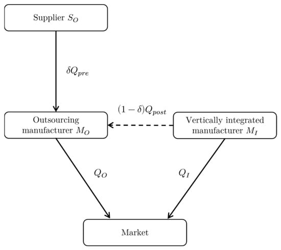
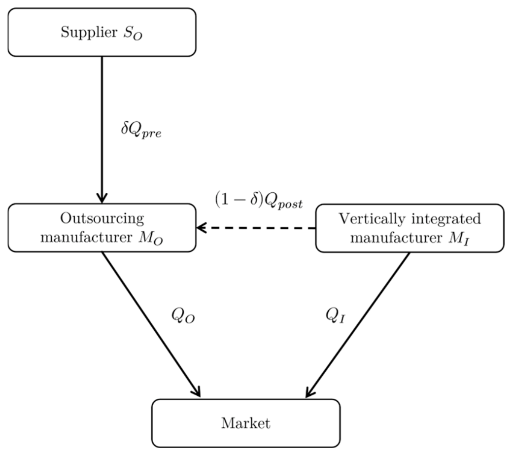
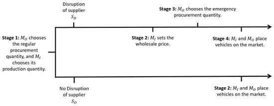
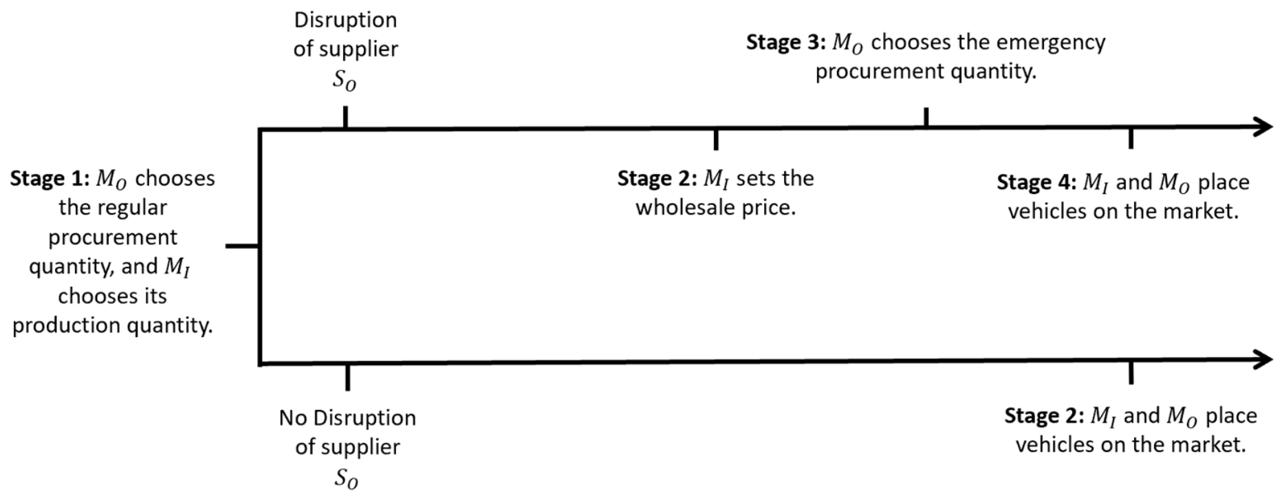
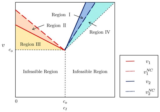
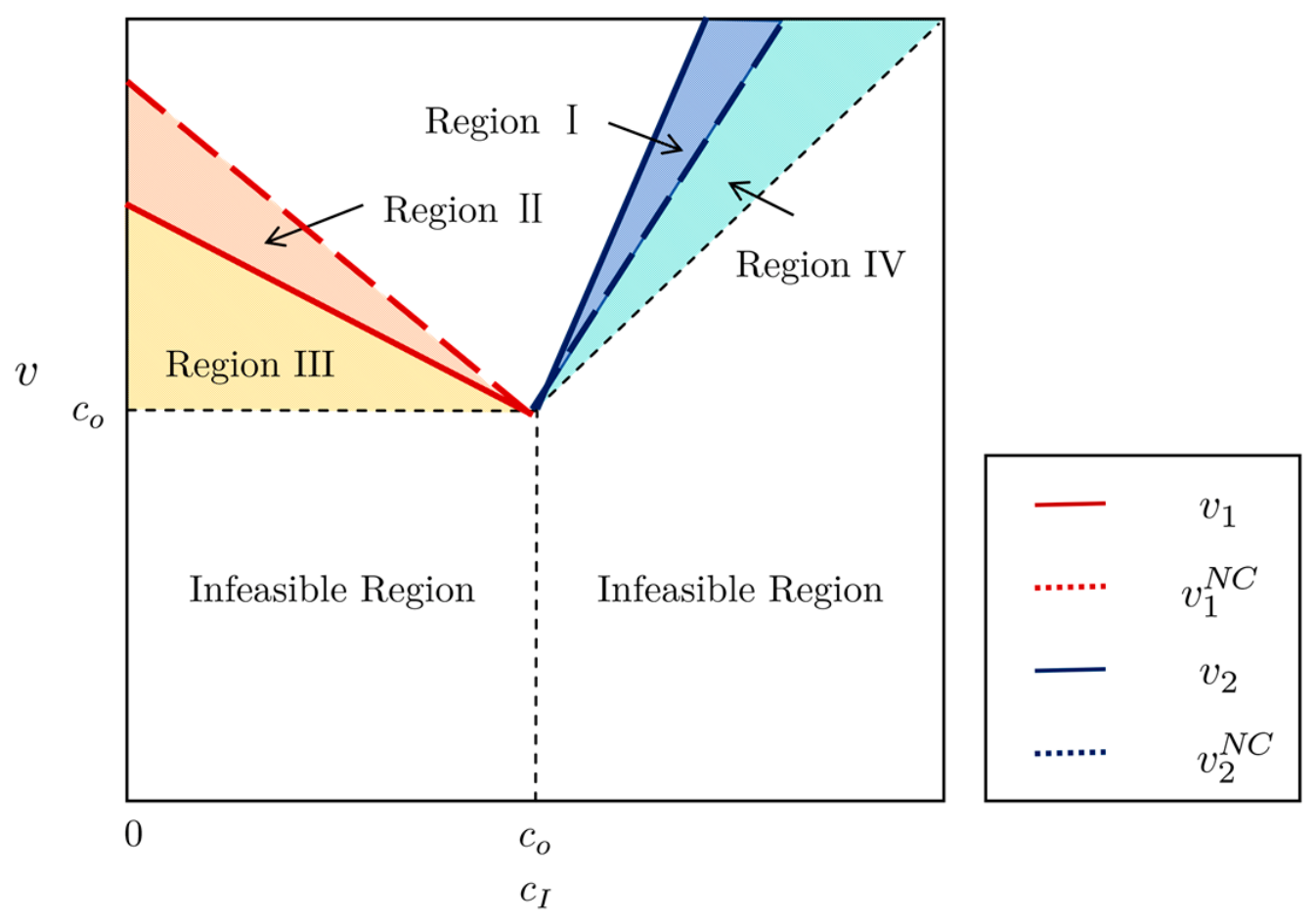
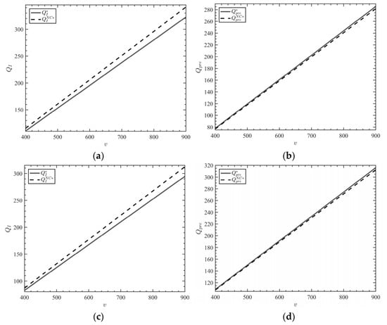
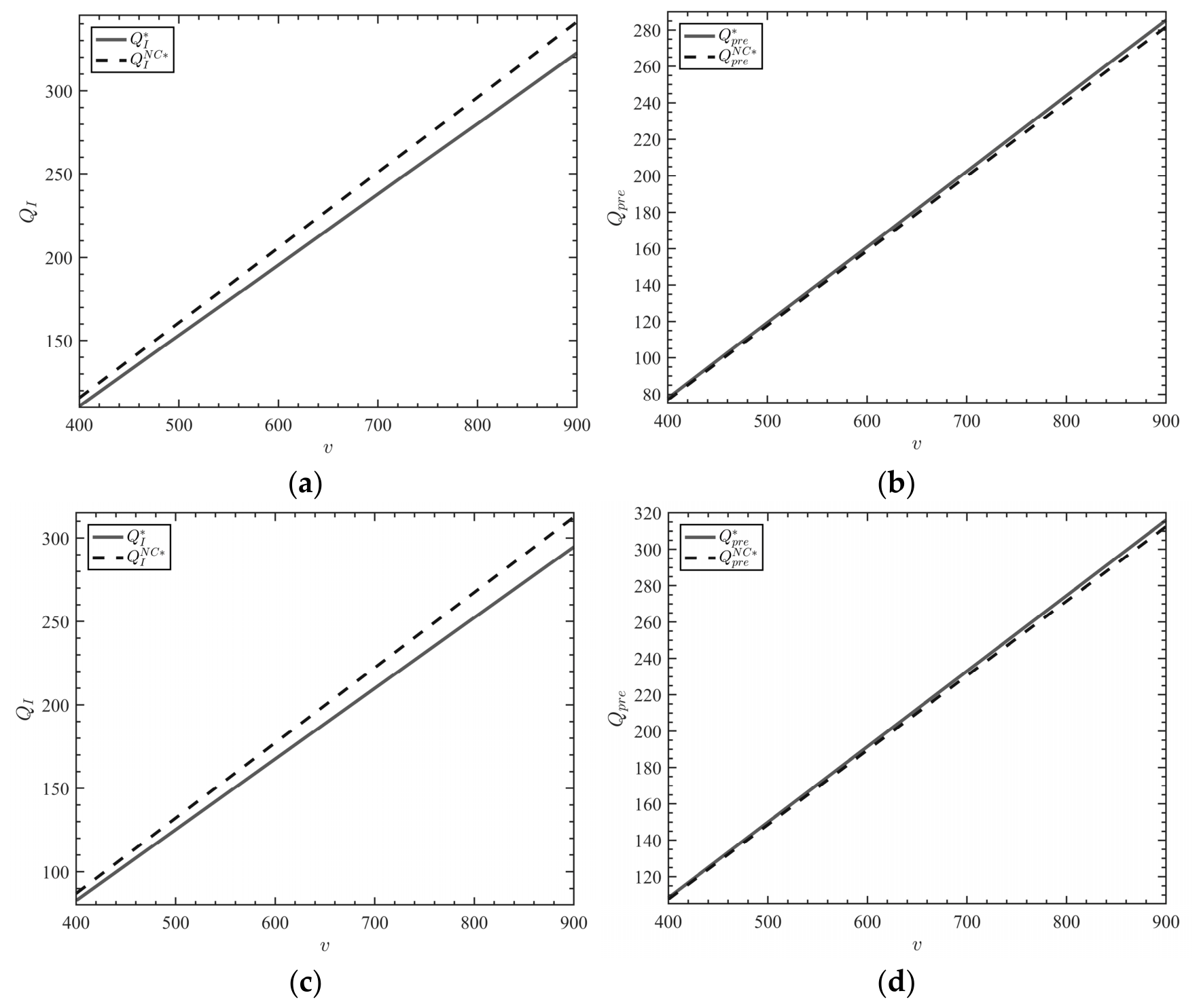
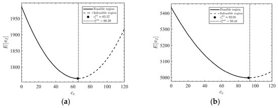
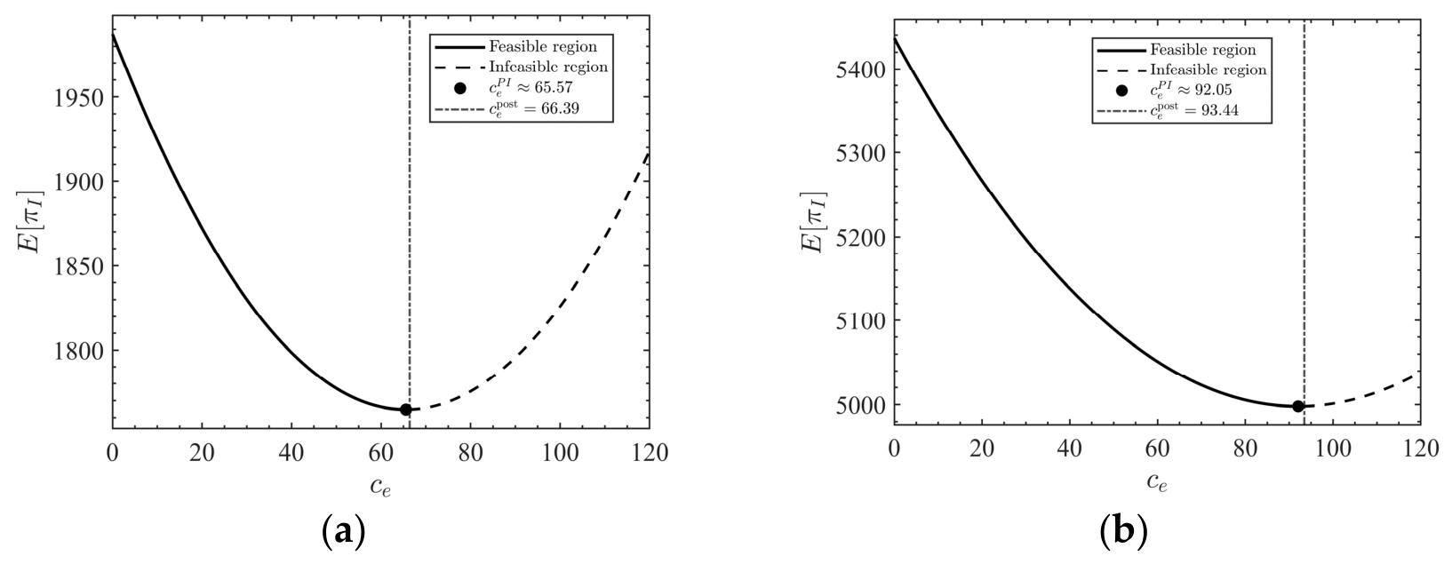
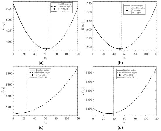
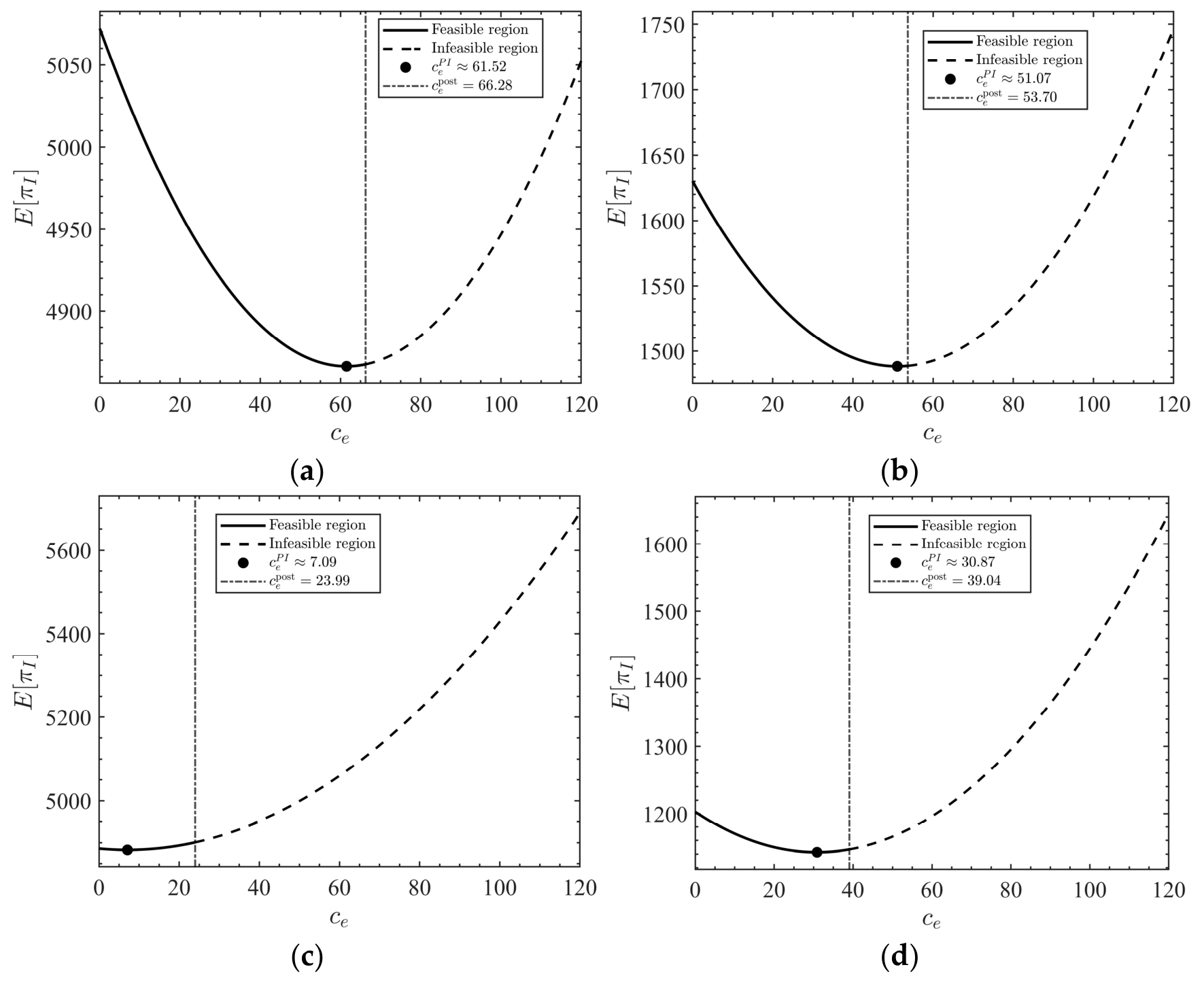
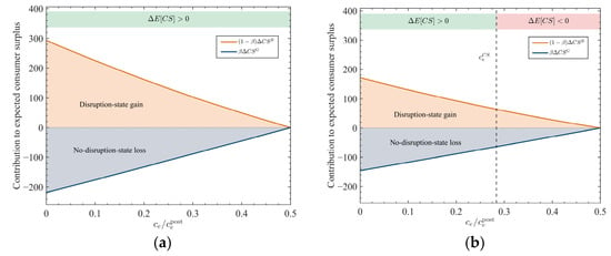
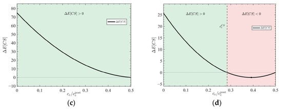
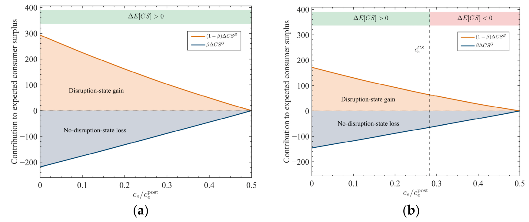
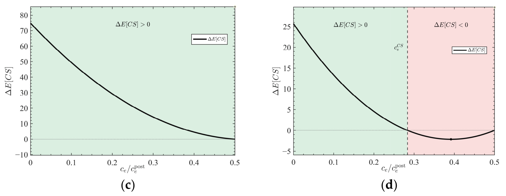
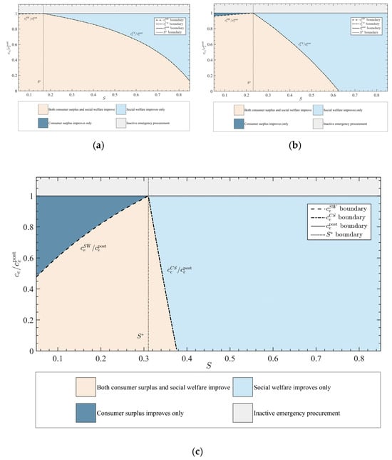
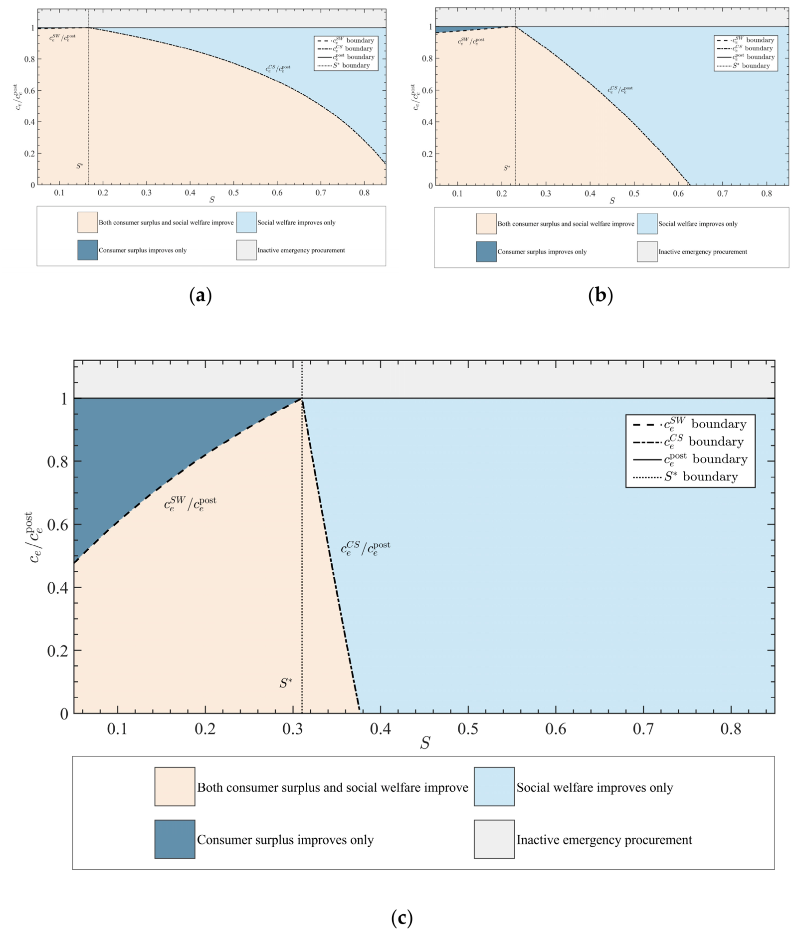

Disclaimer/Publisher’s Note: The statements, opinions and data contained in all publications are solely those of the individual author(s) and contributor(s) and not of MDPI and/or the editor(s). MDPI and/or the editor(s) disclaim responsibility for any injury to people or property resulting from any ideas, methods, instructions or products referred to in the content. |
© 2026 by the authors. Licensee MDPI, Basel, Switzerland. This article is an open access article distributed under the terms and conditions of the Creative Commons Attribution (CC BY) license.