


Highlights
Please indicate how your work links to systems science via your contributions to systems practice, theory, and/or methodology.
- This study analyzes trade-in insurance in a product upgrade and recovery system.
- The model links customer decisions with product sales, rebate obligations, return flows, and recovery value.
What are the main findings and/or the implications of the main findings?
- Trade-in insurance changes customer segmentation and the joint design of the insurance price and trade-in rebate.
- Distinct customer paths can generate the same aggregate operational flows and optimal policies.
Abstract
This paper develops a two-period analytical model of trade-in insurance and rebate design in a product upgrade and recovery system with successive product generations. In standard trade-in programs, customers face uncertainty about future rebate eligibility because rebates depend on the condition of the used product at the upgrade stage. We study an optional insurance mechanism through which customers prepay a fixed fee and receive a guaranteed future trade-in rebate. Customers are financially risk-neutral, but insurance may generate a first-period non-monetary psychological benefit: once future rebate eligibility is guaranteed, customers can use the product during the first-period ownership stage with less anxiety about an unexpected failure eliminating their future trade-in opportunity. Under the baseline specification in which this psychological benefit increases with product valuation, trade-in insurance generates valuation-based customer segmentation among insured upgraders, uninsured trade-in customers, product keepers, delayed buyers, and non-buyers. This insured–uninsured single-crossing result extends to general increasing psychological-benefit functions, including concave forms. The model further shows that the insurance price and trade-in rebate should be coordinated because both instruments affect customer upgrade behavior, product sales, rebate obligations, return flows, and recovery value. When product innovation is sufficiently high, customers no longer keep functional used products, and the optimal insurance price and trade-in rebate become independent of innovation and durability. Compared with a standard trade-in program, optional trade-in insurance weakly improves manufacturer profit, while the economic magnitude of the gain depends on market and operational conditions.
1. Introduction
Trade-in programs have become an important mechanism in product upgrade and recovery systems. By offering customers a rebate for returning a used product when purchasing a new-generation product, manufacturers can stimulate repeat purchases, accelerate product replacement, and recover residual value from returned products through refurbishment, resale, remanufacturing, or recycling [1]. Such programs are widely used in durable-goods and technology-intensive markets, including electronics, automobiles, and home appliances [2]. For example, firms such as Apple and Samsung use trade-in credits to encourage customers to upgrade to newer product generations [3]. At the operational level, trade-in programs connect forward sales, customer replacement behavior, reverse logistics, and product recovery operations [4].
However, trade-in programs also create an important design challenge. A high uniform rebate can be costly for the manufacturer because returned products differ in condition and recovery value. In practice, manufacturers often adjust trade-in rebates according to the quality or condition of the returned product [5]. For example, Samsung evaluates device condition before determining the eligible trade-in value [6]. Although condition-based rebates help the manufacturer control recovery costs, they also create uncertainty for customers. At the time of the initial purchase, customers do not know whether their product will remain functional when the next-generation product becomes available. If the product remains functional and retains sufficient residual value, they may keep it rather than trade it in. If the product fails, they may lose eligibility for the trade-in rebate. This uncertainty may weaken the effectiveness of the trade-in program by making future upgrade value uncertain.
To address this issue, manufacturers may introduce trade-in insurance as a complementary service. Under this mechanism, customers pay a fixed insurance fee at the beginning and receive a guaranteed trade-in rebate later. A similar practice can be observed in the market. For example, OnePlus introduced the OnePlus Assured Upgrade Program in India, under which customers could pay an additional fee and receive a guaranteed buyback value when upgrading to a future flagship device [7]. Samsung’s New Galaxy Club provides a similar mechanism: eligible customers pay a monthly club fee and may later upgrade by trading in the original device for a predetermined upgrade benefit. In the UK, Samsung guarantees 50% of the original device price when customers upgrade between months 12 and 15 [8]. These programs are commercial examples that motivate the contractual structure studied in this paper: customers make an additional payment in exchange for a predetermined future upgrade or buyback benefit. They are not used as empirical evidence for the model’s predicted customer segmentation, regime thresholds, rebate responses, or profit effects. The present study is theoretical, and empirical validation of these predictions requires customer- or transaction-level data.
Trade-in insurance provides customers with two kinds of benefits. First, it provides financial protection by guaranteeing the trade-in rebate if an unexpected product failure would otherwise eliminate rebate eligibility. Because the rebate is realized in the second period, this financial value depends on the failure probability, rebate amount, and intertemporal discount factor. Second, insurance may generate a non-monetary psychological benefit during first-period ownership. Prior research indicates that insurance can provide peace of mind, reduce anticipated regret, and improve subjective well-being before uncertainty is resolved [9,10,11].
Although the trade-in transaction occurs in the second period, uncertainty about future rebate eligibility affects customers from the beginning of product ownership. Without insurance, a customer uses the product while knowing that an unexpected failure or deterioration may eliminate the future trade-in opportunity. After purchasing insurance, the customer knows that such a failure will not result in the loss of rebate eligibility and can therefore use the product during the first period with less anxiety about its future condition. The psychological benefit begins when coverage is purchased and continues throughout the first-period usage stage. It is therefore modeled as first-period anticipatory utility rather than as a second-period payoff.
Motivated by these insights, we allow insurance to generate a non-monetary psychological benefit that increases with the customer’s valuation of the product. In this study, the psychological benefit is specified as , where u measures the customer’s valuation of the product and its associated upgrade path. This formulation does not imply that higher-valuation customers lose a larger monetary rebate because the trade-in rebate (R) is independent of u. Instead, customers with a higher u attach greater non-monetary importance to preserving access to the future upgrade opportunity and therefore obtain greater current reassurance from guaranteed rebate eligibility. The expected monetary protection is captured separately.
This paper studies a two-period product upgrade and recovery system in which a monopolistic manufacturer sells two successive product generations. Customers are heterogeneous in product valuation and make forward-looking decisions about whether to buy the first-generation product, purchase trade-in insurance, upgrade, trade in, or keep a functional used product. The manufacturer obtains salvage value from returned functional products and jointly determines the insurance price and trade-in rebate to maximize profit.
Methodologically, this paper employs a two-period analytical operations management model. Its systems relevance lies in mapping heterogeneous customer decision paths into interconnected manufacturer-facing flows, including product sales, insurance payments, rebate obligations, product returns, and recovery value. This aggregate-flow representation allows different micro-level customer paths to be compared according to their operational and profit consequences. The model does not employ system dynamics, feedback-loop analysis, or stock–flow accumulation; instead, it provides an analytical representation of how customer decisions affect the forward product market and reverse recovery operations.
The following research questions are examined in this paper:
- How does guaranteed rebate eligibility change customer self-selection across insured upgrading, uninsured trade-in, keeping the current product, delayed purchase, and no purchase, and under what psychological-benefit specifications does the insured–uninsured cutoff remain valid?
- How do the insurance price and trade-in rebate interact to determine the active customer segments and the manufacturer’s profit-maximizing regime?
- For a given product price, how do failure probability, product innovation, used-product durability, customer patience, salvage value, and psychological benefit affect the optimal insurance price, trade-in rebate, and regime boundaries?
- Under what market and operational conditions does trade-in insurance generate a strict and economically meaningful profit gain relative to a standard trade-in program without insurance?
Our analysis shows several findings. First, trade-in insurance allows for more precise customer sorting: under the baseline increase in psychological-benefit specification, high-valuation customers are more likely to purchase insurance for rebate certainty and peace of mind, middle-valuation customers trade in without insurance, and lower-valuation customers either keep their products or delay purchase. Second, the optimal insurance price and trade-in rebate should be jointly determined. They are affected by the product price, salvage value, innovation level, and customer migration across segments. Third, the effect of product durability on the optimal insurance price depends on the innovation level of the updated product. Fourth, optional trade-in insurance cannot reduce the manufacturer’s optimized profit, while the magnitude of the gain depends on market and operational conditions. Finally, distinct customer decision paths can generate the same aggregate operational flow structure. When different customer allocations produce equivalent product sales, insurance payments, rebate obligations, product returns, and recovery value, they enter the manufacturer’s profit function in the same way and may therefore lead to the same optimal decision expressions. This result shows how different micro-level behaviors can produce equivalent system-level operational consequences.
The remainder of the paper is organized as follows. Section 2 reviews the literature on trade-in programs and insurance. Section 3 presents the problem framework, derives customer utility functions and segment demand. Section 4 derives the manufacturer’s optimal insurance price and trade-in rebate and provides sensitivity analysis. Section 5 compares the benchmark cases with and without insurance and also examines the high-innovation case. Section 6 summarizes the managerial insights and future research directions.
2. Literature Review
This study builds on three related streams of research: trade-in programs and product upgrade decisions, warranties and insurance-related protection, and signaling and customer self-selection. The first stream examines how trade-in programs affect product replacement, pricing, customer migration, and product recovery. The second stream studies why customers purchase optional protection and how firms price such services. The third stream provides a theoretical interpretation of insurance adoption as an observable customer choice that can reveal private willingness to pay. Together, these streams clarify the position of trade-in insurance as a mechanism that links rebate certainty, customer behavior, product upgrading, and recovery operations.
2.1. Trade-In Programs and Product Upgrade Decisions
Trade-in programs connect new-product sales with customer replacement decisions and used-product recovery. Yin et al. (2015) [12] study the pricing of two successive product generations under uncertainty and show that a future trade-in option can affect the timing of the initial purchase. Hu et al. (2019) [2] examine optimal prices and trade-in rebates when strategic customers face a limited trade-in period. Agrawal et al. (2016) [5] show that trade-in rebates can support both price discrimination and product recovery. These studies establish that trade-in programs are not simply promotional discounts; they also influence intertemporal purchase decisions and reverse product flows.
Subsequent studies extend trade-in decisions to more complex market and operational settings. Feng et al. (2019) [13] investigate trade-in pricing in a dual-channel supply chain and show how market segmentation and channel power affect the performance of the program. Li et al. (2019) [14] examine how a secondary market affects pricing, trade-in remanufacturing, and market-entry decisions. Feng et al. (2025) [15] further consider the joint choice of product price and quality when a secondary market and a trade-in program coexist. Li et al. (2022) [16] study the manufacturer’s choice between retailers and collection platforms as trade-in partners, while Bai et al. (2023) [17] examine trade-in mode selection in the presence of resale platforms. Guo et al. (2025) [18] analyze the interaction between trade-in modes and government subsidies, and Yang and Liu (2024) [19] investigate trade-in strategies under sequential product innovation.
Sheu and Choi (2019) [20] provide the closest behavioral comparison to the present study. They examine competing trade-in-for-upgrade programs through a multi-method approach and incorporate reference-dependent choice, market competition, green value, and extended consumer responsibility. In their framework, customer participation depends on the perceived value of the new product, the residual value of the used product, prices and rebates, and green-value considerations. Their main concern is how competing firms design pricing and rebate policies while creating firm, customer, and environmental value.
The present study differs from the framework of Sheu and Choi (2019) [20] in both the source of uncertainty and the behavioral mechanism. We do not model reference dependence, green-value preferences, or competition between alternative trade-in programs. Instead, customers face uncertainty about whether the condition of their product will satisfy the future rebate requirement. The manufacturer offers an optional, fee-based insurance contract that guarantees rebate eligibility. The psychological benefit in our model is the first-period peace of mind obtained after this eligibility risk has been removed. The manufacturer then jointly determines the insurance price and trade-in rebate. Therefore, the insurance decision affects not only perceived customer value but also insurance adoption, upgrading, rebate obligations, product returns, and recovery value.
2.2. Warranties, Insurance, and Psychological Protection
Classical insurance theory provides the foundation for understanding the value of protection. Mossin (1968) [21] relates insurance demand to risk aversion, loss probability, coverage, and premium loading. Rothschild and Stiglitz (1978) [22] examine competitive insurance markets under asymmetric information and show how privately informed customers may self-select among different insurance contracts. Their analysis provides a theoretical foundation for understanding how observable contract choices can separate customer types. These studies establish that insurance pricing depends on contract design. The present model does not rely on financial risk aversion. Customers in our model are financially risk-neutral, and the expected financial benefit of insurance is represented separately by the discounted value of the additional rebate received when the product fails.
The literature on warranties and extended warranties is directly relevant because these services also require customers to pay an additional fee for future protection. Maronick (2007) [23] finds that extended warranties can provide both protection from future repair expenses and peace of mind. Jindal (2015) [24] shows that loss aversion is an important driver of extended-warranty demand and that warranty pricing can help firms discriminate among customers with different willingness to pay. Estelami et al. (2016) [25] identify determinants of extended warranty prices by using a large dataset, which indicates that product price, category, expected service cost, and market factors can affect the price.
Trade-in insurance resembles an extended warranty because both are optional, fee-based forms of future protection. However, the protected object and the operational consequences differ. A warranty generally pays for or provides repair, replacement, or related service after product failure. Trade-in insurance does not repair the product or compensate the customer for repair expenses. It protects the customer’s eligibility for a future trade-in rebate and becomes valuable when the customer follows the upgrade path. It therefore directly affects second-period product sales, rebate payments, product returns, and recovery operations. This distinction explains why warranty pricing results cannot be applied directly to the joint design of the insurance price and trade-in rebate.
Behavioral insurance research further shows that the value of protection is not limited to its expected monetary payoff. Braun and Muermann (2004) [9] connect insurance demand with anticipated regret. Tafere et al. (2019) [10] identify peace-of-mind and buyer’s-remorse effects associated with insurance coverage, while Rieger-Fels (2024) [11] discusses behavioral explanations for insurance purchases beyond conventional risk aversion. Chi and Zhuang (2022) [26] incorporate regret preferences into optimal insurance design.
These studies support the distinction between financial protection and non-monetary psychological protection in our model. The guaranteed rebate is realized in the second period, so its expected financial value depends on the failure probability, the rebate, and the discount factor. By contrast, peace of mind begins after the customer purchases insurance and is experienced while the product is used in the first period. It is therefore modeled as part of the first-period utility. This timing is also consistent with the anticipatory-utility literature, which recognizes that expectations about future outcomes can generate current utility or disutility before the underlying uncertainty is resolved [27,28].
2.3. Signaling, Self-Selection, and Insurance Adoption
Theories of signaling and self-selection help explain how optional insurance can reveal customer information. In the insurance literature, Rothschild and Stiglitz (1978) [22] show that customers with private information may select different contracts, allowing observable contract choices to separate customer types. More broadly, Yang et al. (2025) [29] use signaling theory to explain how observable actions can convey otherwise hidden attributes to stakeholders and reduce information asymmetry.
Insurance prices can also transmit information in the opposite direction. Reiner et al. (2025) [30] show that customers may interpret a high insurance price as a signal that the underlying product is risky. Their mechanism is therefore a firm-to-customer signal: the insurance price affects customers’ beliefs about product risk. The mechanism in our study is different. The manufacturer does not observe each customer’s valuation directly, but it observes whether the customer purchases insurance. Because buying insurance is costly and its psychological benefit increases with product valuation in the baseline model, high-valuation customers are more willing to purchase it. Insurance adoption therefore acts as a customer-to-manufacturer self-selection signal.
This mechanism produces a valuation-based separating outcome between insured and uninsured customers. The manufacturer does not learn each customer’s exact valuation; it learns whether the customer’s willingness to pay lies above the insurance-adoption threshold. The insurance price controls the location of this threshold, while the trade-in rebate affects both the financial value of coverage and the attractiveness of uninsured trade-in. The two instruments must therefore be coordinated. This signaling interpretation provides the theoretical basis for the customer-segmentation result, although the model is not intended to represent a general signaling game with multiple firms or supply chain partners.
2.4. Research Gap and Positioning
The above literature provides important foundations for understanding trade-in rebate design, product replacement, customer upgrade behavior, and insurance demand. However, three research gaps motivate this paper.
First, existing trade-in studies mainly examine how rebates affect replacement behavior, pricing, channels, and recovery. They pay less attention to the uncertainty customers face at the initial purchase stage about whether their product will remain eligible for a future rebate. This uncertainty links the product’s future condition to current purchase and insurance decisions.
Second, warranty and insurance studies explain financial protection, peace of mind, regret, and self-selection, but they generally do not connect these mechanisms to a condition-dependent trade-in rebate and the resulting product upgrade and recovery flows. Trade-in insurance differs from conventional product protection because its payoff is tied to a future upgrade transaction rather than to repair or replacement alone.
Third, prior research provides limited guidance on how a manufacturer should jointly design an insurance price and a trade-in rebate. The insurance price determines which customers purchase protection, while the rebate affects insured and uninsured upgrading, the manufacturer’s rebate obligations, and the quantity of returned products. Optimizing either instrument alone would overlook their interaction.
Accordingly, the contribution of this paper is not merely to add insurance to an existing trade-in model. It integrates rebate-eligibility uncertainty, first-period psychological protection, customer self-selection, forward product sales, and reverse product recovery within one two-period analytical framework. The analysis identifies when customer segments are active, how the manufacturer should coordinate the insurance price and trade-in rebate, and how this coordination changes product sales, rebate payments, return flows, recovery value, and profit. It also states the boundary of the segmentation result: high-valuation customers are more likely to purchase insurance when the psychological value of rebate certainty increases with valuation. This integrated treatment explains how a customer-facing insurance decision changes both market demand and recovery-related operational outcomes.
3. Modeling
In this section, we first present the problem framework and then derive the demand functions for different customer segments based on the utility theory.
3.1. Product Upgrade and Recovery System Framework
We consider a product upgrade and recovery system operated by a monopolistic manufacturer over two periods. The system consists of a manufacturer, heterogeneous customers, two successive product generations, an optional trade-in insurance contract, a trade-in rebate, and a recovery channel for returned products. The manufacturer sells the first-generation product in the first period and introduces an updated product in the second period. Customers decide whether to purchase the first-generation product and whether to buy trade-in insurance at the beginning of the first period. In the second period, based on their purchasing behavior in the first period, they decide whether to upgrade, trade in, keep the used product, or purchase the new product. Returned functional products generate recovery value for the manufacturer through recovery activities, depending on product condition.
In period 1, the manufacturer sells the first-generation product at a unit price p. In period 2, an updated product is introduced at the same price p. This uniform pricing assumption is consistent with studies on successive product generations [31,32]. It is a common practice in markets in which companies keep prices stable across generations to simplify pricing and reduce customers’ incentive to delay purchase. For example, Apple did not change the price for several iPhone generations. The lowest-priced iPhone 14 was priced at $799 [33], which was the same as the starting prices of iPhone 15 and iPhone 16 [34]. The product price p is treated as exogenous. The exogenous-price assumption allows the analysis to focus on the interaction between the insurance price and the trade-in rebate. In many product-generation markets, manufacturers maintain relatively stable headline prices across successive versions while adjusting auxiliary instruments such as rebates, upgrade programs, and service contracts. Treating p as fixed therefore isolates the strategic role of trade-in insurance and prevents the model from conflating product pricing with rebate-risk protection. If the product price were also optimized, the manufacturer would have an additional instrument for screening customers, and the optimal policy would depend on the joint interaction among product price, insurance price, and trade-in rebate. We leave this extension for future research. The production cost of the updated product is assumed to be identical to that of the original product and is normalized to zero, which is a common simplification in analytical pricing and supply chain models [35].
Customers are heterogeneous in their valuation of the first-generation product. A customer’s perceived valuation of the product is denoted by u, where u is uniformly distributed on (a similar setting is used by Hu et al. (2023) [36]). The time discount factor is denoted by , which captures the extent to which customers value second-period utility relative to first-period utility. A larger indicates that customers are more patient and place greater weight on future consumption utility.
After one period of use, the product condition becomes uncertain. With probability , the product remains functional, but its perceived value decreases from u to because of normal wear and quality degradation. The parameter represents the durability level of a functional used product. With probability , the product fails completely at the beginning of period 2. In this case, the used product provides no consumption value to the customer, and its perceived value is normalized to zero.
If the used product remains functional, the customer may return it through the trade-in program and receive a rebate R when purchasing the updated product. The manufacturer obtains an average salvage value s from each returned functional product. This salvage value represents the recovery benefit generated through recycling. For failed products, we assume that the salvage value offsets the associated collection and recycling costs, so the net recovery value is normalized to zero.
To reduce customers’ uncertainty about future rebate eligibility, the manufacturer may offer optional trade-in insurance at price in the first period. A customer who purchases insurance is guaranteed to receive the trade-in rebate R when purchasing the updated product in the second period, regardless of whether the used product remains functional or has failed. The customer must surrender the used product to use the guaranteed rebate. Thus, R is an upgrade credit rather than a cash payment independent of product replacement. A functional returned product generates salvage value s, whereas a failed returned product generates zero net recovery value.
We assume that product ownership and condition can be verified and that insurance does not change the customer’s product-use effort or the physical failure probability (). Strategic product damage, false reporting, fraud, and moral hazard are therefore outside the scope of the model.
The manufacturer’s decision variables are the insurance price and the trade-in rebate R. The objective is to design these two instruments jointly in order to influence customer migration across different system states, including insured upgrading, uninsured trade-in upgrading, keeping the functional used product, delayed purchase, and no purchase. The overall product upgrade and recovery system is illustrated in Figure 1.
Figure 1.
Two-period product upgrade and recovery system with trade-in insurance.
3.2. Customer Decision States and Aggregate Demands
Customers are assumed to be financially risk-neutral in this study, which means that they evaluate monetary payoffs by their expected values and do not receive utility directly from monetary risk reduction. However, customers may still receive non-monetary psychological utility from rebate certainty. Therefore, insurance demand in this model is not driven by monetary risk aversion, but by the combined effect of guaranteed rebate eligibility and psychological benefit.
Customers’ decisions determine how demand flows through the product upgrade and recovery system. Depending on their valuation, insurance adoption, and the realized condition of the used product, customers may enter different decision states: insured upgrading, uninsured trade-in upgrading, keeping the functional used product, delayed purchase, or no purchase. These customer states determine product sales in the two periods, insurance payments, rebate obligations, returned-product quantities, and recovery value. Trade-in insurance changes the allocation of customers across these states by guaranteeing future rebate eligibility.
In the first period, the customer faces three different choices: (1) purchase the product with additional insurance, (2) purchase the product only, or (3) purchase nothing.
Although the trade-in transaction and rebate payment occur in the second period, the uncertainty about future rebate eligibility affects the customer from the beginning of first-period ownership. Without insurance, the customer uses the product while knowing that an unexpected failure or deterioration may eliminate eligibility for the future trade-in rebate. This creates an ongoing psychological burden during the first-period usage stage, including concern about the product’s future condition and anticipated regret about losing the upgrade benefit.
Purchasing trade-in insurance removes this eligibility uncertainty. The customer knows that an unexpected product failure will not eliminate the future trade-in rebate. Therefore, the customer uses and enjoys the product during the first-period ownership stage with less anxiety about whether its future condition will prevent participation in the trade-in program. The psychological benefit begins when insurance is purchased and continues throughout the first-period usage stage.
We represent this first-period psychological relief by . The perceived value of the product is u, while captures the additional peace of mind, reduced concern about accidental failure, and lower anticipated regret generated by guaranteed future trade-in eligibility. Thus, the insured customer obtains first-period utility . This formulation does not mean that insurance improves the physical quality of the product. It captures the non-monetary utility generated by using the product with less concern about losing future rebate eligibility.
The benefit is scaled by u because customers who place greater value on the product and its associated upgrade path attach greater importance to preserving access to the future trade-in opportunity. They therefore obtain greater psychological relief from knowing that the opportunity is protected. This is distinct from the expected monetary value of insurance, which is captured separately by . Because the psychological relief is experienced during first-period ownership, it is not multiplied by the intertemporal discount factor .
For any given , an alternative specification in which the same valuation-dependent benefit is realized in the second period and written as is observationally equivalent to the present specification after defining the effective intensity as . Conditional on this effective intensity, the customer utility comparisons, insurance-adoption cutoff, demand expressions, and subsequent analytical results remain unchanged.
By contrast, a psychological benefit proportional to the expected rebate loss, such as , is independent of customer valuation because , , and R are common across customers. It therefore belongs to the fixed-benefit case: it may shift the overall attractiveness of insurance, but it cannot by itself generate valuation-based separation.
We assume that insurance reduces psychological anxiety without changing the customer’s product-use effort or the physical failure probability . Therefore, the model captures peace-of-mind utility rather than moral hazard.
In the second period, customers may purchase the updated product with or without a trade-in rebate, or keep the used product, depending on the second-period product state and utility comparison. The new product generates utility for customers, where indicates the innovation level of the updated product compared with the old-generation product. A high value of indicates that the updated product is more attractive to customers. The customers’ decision process is illustrated in Figure 2.
Figure 2.
Customer decision process across purchase, insurance, upgrade, trade-in, and keeping states.
Being forward-looking, each customer anticipates the situation in the second period and chooses the action that maximizes the overall utility over two periods. Six customer segments arise from these purchase decisions, as listed below.
- Insured trade-in upgraders who buy products in period 1 with the insurance and trade in period 2 (Option BB).The customer pays in the first period. During first-period ownership, the customer obtains the intrinsic product-use utility u and the additional psychological benefit from knowing that an unexpected failure will not eliminate future trade-in rebate eligibility. The total first-period utility is therefore
- Insured keeper, who buy products in period 1 with the insurance, and keep the functional product in the period 2 (Option BIK).The customer pays in the first period. During first-period ownership, the customer obtains product-use utility u and the psychological benefit from guaranteed future rebate eligibility. If the product fails in the second period, the customer uses the insured rebate to purchase the updated product; if it remains functional, the customer keeps the old product. The total utility is
- Uninsured upgraders, who buy products in period 1 without insurance, and trade in in period 2 (Option BT).The customer pays p in period 1 and gets u. In period 2, if the product is still functional, he trades in the used product and receives R for purchasing the new product. Otherwise, he purchases the new product without the rebate. The total expected utility is
- Uninsured keepers, who buy products in period 1 without insurance, and keep functional products in period 2 (Option BK).The customer buys at price p in period 1, uses the product in both periods, and never trades in. In period 2, if the product is still functional, he obtains ; if it has failed, he needs to buy the updated product without the rebate. The expected utility is
- Delayed buyers, who make no purchase in period 1 but purchase updated products in period 2 (Option NB).The customer makes no purchase in period 1 and in period 2. He buys the new product at price p and enjoys . The discounted utility is
- Non-buyers make no purchase in either period and obtain zero utility (Option N).
A strategic customer makes the purchase decision, which can maximize the utility over the two periods. By comparing Equations (1)–(5), we obtain the results in Lemma 1 and Figure 3.
Figure 3.
Customers’ segments when and .
Lemma 1.
The optimal decisions of the prospective customer in the case and :
- if , option BB is optimal;
- if , option BT is optimal;
- if , option BK is optimal;
- if , option NB is optimal;
- if , option N is optimal;
Lemma 1 shows that customers can be segmented into different groups based on their initial valuation u on the first-generation products. High-valuation customers are willing to pay for insurance, allowing the manufacturer to extract additional profit via . Medium-valuation customers trade in without insurance. Lower-medium customers keep the functional product in the second period, avoiding a costly upgrade, while lowest-valuation customers delay purchase to the second period. The manufacturer can adjust R to encourage trade-in and thus also boost second-period demand or lower to make insurance more attractive to customers. Additionally, other parameters can also shift the segmentation: a higher probability of failure or the intensity of this psychological benefit increases the value of insurance, while a higher innovation level makes delay more attractive, so the manufacturer must balance these forces to avoid losing too many early sales or cannibalizing future profits.
We consider a more general case. Let denote a general psychological benefit from purchasing trade-in insurance. Comparing an insured upgrader with an otherwise identical uninsured upgrader gives
Proposition 1.
Suppose that is continuous and strictly increasing in u. The insurance-adoption decision satisfies a property: If lies within the range of , there exists a unique cutoff
such that customers with prefer insured upgrading to uninsured upgrading.
Proposition 1 shows that the single-crossing property between insured and uninsured upgraders does not require the linear specification . It only requires the psychological benefit from rebate certainty to be continuous and strictly increasing in customer valuation.
For example, under the normalized concave specification , where , define The insurance-adoption cutoff is , whereas the corresponding cutoff under the linear specification is . Because and , we have Thus, the concave specification extends insurance adoption to some lower-valuation customers. It preserves the insured–uninsured single-crossing property but makes insurance less selective with respect to valuation. This is the specific sense in which concavity weakens valuation-based separation.
The scope of Proposition 1 is limited to the pairwise comparison between insured and uninsured upgraders. The remaining thresholds involving keepers, delayed buyers, and non-buyers have not been re-derived under a general increasing . Therefore, the full five-segment ordering in Lemma 1, the associated demand functions, and the exact regime boundaries used in the subsequent analysis remain based on the linear baseline specification .
This sorting result depends on the psychological benefit increasing with customer valuation. If the benefit is fixed across customers, including a benefit proportional only to the expected rebate loss, the utility difference between insured and uninsured upgrading does not vary with u. Such a benefit may change aggregate insurance adoption, but it does not by itself generate valuation-based separation. If the benefit is unrestricted and heterogeneous across customers, the single-crossing property may fail unless the benefit remains ordered with customer valuation.
Corollary 1.
Compared to the results in Lemma 1, when the price of the insurance is sufficiently low (), the customers’ structure switches from and to and around the intermediate valuation range.
This corollary shows that a low insurance price expands insurance adoption across two margins (see Figure 4). Customers who would trade in without insurance now purchase insurance and enter the segment due to the lower insurance price. Moreover, some customers who would keep a functional old product would also purchase insurance and enter the segment to decrease the expected loss due to failure. For these customers, insurance mainly serves as failure protection rather than as a trade-in incentive.
Figure 4.
Customer segmentation when the insured-keeper segment is active.
Corollary 2.
Compared to the results in Lemma 1, when , BK segment disappears.
When the innovation level of the updated product is sufficiently low, some customers may prefer to keep the first-generation product if it remains functional, because the residual value of the used product (customer’s side), captured by , is sufficiently attractive relative to the value of upgrading. However, when is sufficiently high, the updated product generates a large utility improvement over the old generation. In this case, even a functional used product becomes less attractive, since keeping it requires customers to forgo the substantial value created by the new-generation product. Therefore, the BK segment disappears from equilibrium (see Figure 5).
Figure 5.
Customer segmentation when high innovation eliminates the uninsured-keeper segment.
In the following analysis, we focus on the customer segments characterized in Lemma 1. Under its insurance-price condition, option BIK is not optimal; therefore, the insured-keeper segment is empty (). This segment may become active when the insurance price is sufficiently low, as shown in Corollary 1 and Section 5.4. The high-innovation case is examined in Section 5.3. Because u is uniformly distributed on , the segment demands are as follows:
The notation used in this model is summarized in Table 1.
Table 1.
Notation in the model.
4. Mathematical Model and Equilibrium Analysis
This section characterizes the manufacturer’s optimal pricing and rebate decisions for the trade-in service. We first formulate the manufacturer’s profit-maximization function, then establish the analytical properties of the model.
4.1. Optimal Insurance-Pricing and Rebates Decision
The manufacturer optimizes the total profit over two periods by adjusting the trade-in rebate (R) and the price () for the trade-in insurance. The mathematical model is listed below:
The objective function (12) includes four profit components. Each represents the profit the manufacturer generates from one customer segment. Constraint (13) is used to prevent unlimited purchase. If , a customer could buy the product in period 1 (paying p) and then get a free updated product, since the trade-in rebate R is sufficiently high. Constraints (14) and (15) guarantee that all demands and decision variables are non-negative.
Lemma 2.
For , the manufacturer’s profit function is jointly concave in the insurance price and the trade-in rebate R if and only if , where
The condition guarantees that the Hessian matrix is negative semidefinite and that the KKT conditions are sufficient for identifying a global optimum. It is not, however, a condition for the existence of an optimal solution. For every , the demand constraints, , and define a closed and bounded feasible set. Therefore, a global profit-maximizing solution continues to exist when . The threshold increases with the failure probability and innovation level , while it decreases with the discount factor and durability level of a functional used product . Thus, the restriction is most relevant for products with high failure probability, relatively impatient customers, strong product innovation, and low residual durability.
Under the illustrative parameter values used in the following, , , , and , the threshold is which is of the order of six ten-thousandths. Therefore, the concavity restriction binds only weakly under the benchmark parameter values. However, because increases proportionally with , the threshold rises rapidly when the product failure probability is large. The condition may therefore become economically restrictive for products with a very high failure probability.
Corollary 3.
When , no strictly interior feasible solution satisfying
can be a local or global profit maximum. Consequently, every global maximizer must satisfy at least one binding constraint:
When , the determinant of the Hessian matrix is negative, so the Hessian has one positive and one negative eigenvalue. A strictly interior profit maximum must satisfy the first-order conditions, but any such stationary point is a saddle point and can therefore be improved along a feasible direction. The global optimum must instead be obtained by optimizing profit along the feasible boundaries and comparing the resulting boundary candidates and their intersections. Under this situation, the fully interior solution (Regime 4 in the following) cannot be optimal in the non-concave region, which is a key part in the following discussion. Therefore, the related results below are conditional on this constraint .
By solving the model, we derive the manufacturer’s optimal decisions, which are summarized in Proposition 2 and Figure 6.
Figure 6.
Optimal regime classification in the space.
The manufacturer’s optimization problem is characterized by different active demand segments. Because the insurance price and trade-in rebate R jointly determine the boundaries among insured upgraders, uninsured trade-in upgraders, and uninsured keepers, the optimal solution may occur either in the interior of the feasible region or on a boundary where one or more customer segments disappear. Therefore, the equilibrium can be classified according to which customer segments remain active under the optimal policy. This regime-based characterization is useful because it links the mathematical solution to the system structure: each regime represents a different configuration of product sales, insurance adoption, trade-in participation, and product recovery.
Proposition 2.
The manufacturer’s optimal strategy falls into one of the six regimes summarized in Table 2.
Table 2.
Regime-demand mapping for Proposition 2.
Proposition 2 shows that the manufacturer’s optimal policy is regime-dependent. The six regimes represent different operational configurations generated by the joint effects of the insurance price and trade-in rebate R on customer allocation. When a segment has zero demand, the corresponding boundary constraint is binding; when it has positive demand, the manufacturer balances the marginal revenue and marginal cost associated with that customer flow.
Regime 1 (R1) represents a standard trade-in outcome in which insurance is not adopted and only uninsured trade-in customers remain active. Regime 2 (R2) describes coexistence between insured and uninsured trade-in customers, but no customers keep functional used products. Regime 3 (R3) represents the case without insurance adoption, where some customers trade in and others keep their functional products. Regime 4 (R4) is the most general interior case: insured upgraders, uninsured trade-in customers, and uninsured keepers all coexist. Regime 5 (R5) corresponds to full insurance adoption among first-period buyers, while Regime 6 (R6) includes insured upgraders and uninsured keepers but no uninsured trade-in segment.
Figure 6 visualizes the analytical regime conditions reported in Table 2 in the space. The parameter values are , , , , and . These values lie within the admissible parameter ranges and provide a moderate benchmark under which the six regime conditions can be clearly illustrated. They are selected for theoretical illustration rather than empirical calibration. Under these parameters, all relevant regime transitions occur within , where . We also numerically verified the full theoretical domain and found that values above neither generate additional regimes nor alter the qualitative regime classification. Accordingly, the horizontal axis is displayed over to improve the visibility of the regime boundaries; the analytical classification remains conditional on .
Figure 6 reveals two main patterns. First, when the psychological benefit is relatively weak, the no-insurance regimes R1 and R3 arise over substantial portions of the moderate- and high-price ranges, whereas R6 appears in the low-price range. As increases, insurance becomes a more effective customer-segmentation instrument, and the regions associated with R2, R4, and R5 become more prominent. A higher increases customers’ willingness to pay for rebate certainty and peace of mind, especially among high-valuation customers. As a result, insurance becomes a more effective self-selection instrument: the manufacturer can obtain additional surplus from high-valuation customers through while using R to control the size of the uninsured trade-in and keeping segments. Therefore, the optimal strategy is determined by the interaction between product margin, insurance valuation, rebate cost, and customer migration across segments.
Second, the product price p determines whether keeping a functional used product remains part of the equilibrium. Lower product prices are generally associated with regimes containing the keeper segment, including R3, R4, and R6. At lower product margins, the manufacturer has less scope to offer a sufficiently attractive trade-in rebate, and some customers therefore retain their functional used products. Higher product prices provide a larger product margin and support more trade-in-oriented regimes, including R1, R2, and R5. However, the specific transition also depends on the value of , because a stronger psychological benefit increases customers’ willingness to pay for rebate certainty and makes insurance adoption more attractive.
Lemma 3.
An increase in the failure probability and the durability level of a functional used product enhances the attractiveness of the insurance, whereas a higher innovation level and a greater period discount factor reduce it.
For a given value of and within the feasible price range examined in Section 4, represents the insurance-exit threshold. Although R1 and R3 involve different combinations of thresholds in Table 2, only determines which no-insurance regime applies: conditional on , leads to R3, whereas leads to R1. This result is consistent with the R5 region in Figure 6, because the insurance-exit threshold depends on . When is high, a product price that is high in absolute terms may still remain below and therefore support R5. Consequently, insurance becomes unattractive when the product price is high relative to the -dependent threshold, an outcome that is especially likely when is relatively low.
A higher failure probability increases the value of insurance because uninsured customers face a greater chance of losing rebate eligibility in the second period. A higher durability level of a functional used product makes the functional used product more valuable to customers; the manufacturer may need to provide a more attractive trade-in arrangement, which also increases the value of guaranteed rebate protection, to induce these customers to upgrade.
In contrast, a higher innovation level reduces the incremental role of insurance. When the updated product is highly attractive, customers already have a strong incentive to upgrade, so the guaranteed rebate becomes less important in driving the upgrade decision. A higher discount factor has a similar effect. Customers place more weight on second-period consumption from the updated product, which reduces the relative importance of insurance as an additional incentive. Therefore, insurance is most attractive when customers face high failure risk or high value from keeping the old product, and less attractive when the new product itself already provides a strong upgrade incentive.
Lemma 4.
A higher salvage value increases the attractiveness of trade-in service for the customers.
represents the threshold above which all customers who purchase the product in the first period are willing to participate in the trade-in program. The increased salvage value of the used product s decreases this threshold. It indicates that a higher salvage value increases the attractiveness of the trade-in service. When returned functional products generate greater recovery value, the manufacturer can benefit more from collecting used products. This gives the manufacturer an incentive to offer a higher trade-in rebate, which encourages more first-period buyers to return their functional used products instead of keeping them.
From the customer’s perspective, a higher rebate reduces the effective cost of upgrading to the new-generation product. As a result, the trade-in option becomes more attractive relative to keeping the used product. Thus, salvage value strengthens the trade-in channel by improving the manufacturer’s recovery benefit and allowing the manufacturer to use rebates more aggressively to stimulate second-period upgrades.
4.2. Sensitivity Analysis
This subsection examines how the equilibrium outcomes respond to changes in key system parameters, including the product price p, psychological benefit intensity , failure probability , innovation level , used-product durability , and salvage value s.
We focus on the comparative statics of the fully interior Regime 4, in which insured upgraders, uninsured trade-in customers, and uninsured keepers all coexist. Accordingly, all results in this subsection are conditional on and on the feasibility conditions of Regime 4, including , , , , and . When , Regime 4 cannot be optimal and the manufacturer’s policy is determined by a boundary solution. The interior comparative statics derived below therefore should not be extrapolated to the non-concave region.
Lemma 5.
Increasing selling price of the product results in increasing insurance price and trade-in rebates.
The increasing price of the products implies that the customer who purchases it has a higher perceived value on it. The insurance provides psychological benefits, and the benefit grows with the value of the product in the customer’s mind. Therefore, the high-valuation buyers are willing to pay a higher price to get the insurance. The manufacturer recognizes this increased willingness-to-pay and raises the insurance price to capture part of the extra surplus.
Moreover, the increasing selling price of the product makes upgrading to the new product more expensive, which discourages buyers in the first period from trading in their used products in the second period. To improve sales in the second period, the manufacturer increases the trade-in rebate, which effectively lowers the upgrading cost and makes the upgrade product more attractive for customers.
Lemma 6.
The impact of the psychological benefit intensity (ϕ) on the manufacturer’s optimal decision is shown in Table 3.
Table 3.
Impact of on the optimal price, rebates, and demands.
Figure 7 visualizes the two comparative-static cases identified in Lemma 6. The parameter values are , , , , and . We consider two fixed product prices, and , and vary the psychological-benefit intensity over . Throughout this interval, the lower-price case satisfies , whereas the higher-price case satisfies . Thus, the two panels remain strictly inside Regime 4 and represent the two price regions of Lemma 6. As increases, increases and decreases when , whereas both and decrease when .
Figure 7.
Effects of psychological benefit intensity on the optimal insurance price and trade-in rebate in two price regions.
The relatively narrow range of in Figure 7 follows from the need to preserve these conditions simultaneously for two fixed product prices. All critical price thresholds are functions of , so changing affects not only the optimal decisions but also the admissible price regions. For the higher-price case, at approximately . At this point, , and the solution becomes a strictly interior Regime 4 solution only when . At the other end, at approximately . Beyond this point, the case no longer belongs to the higher-price subregion and therefore no longer represents the second comparative-static case in Lemma 6. The common interval that maintains strict Regime 4 feasibility and keeps the two fixed prices on opposite sides of is therefore approximately . The plotted interval covers approximately 90% of this common admissible window. Hence, the narrow horizontal range is generated by the joint regime-feasibility and comparative-static conditions rather than by an arbitrary restriction of the numerical analysis.
Lemma 6 and Figure 7 indicate that the insurance product functions as a strategic buffer, effectively absorbing shifts in customers’ psychology and translating them into optimal adjustments of the trade-in rebate. In general, an increase in raises the psychological benefit from insurance, making customers willing to pay more for it. The manufacturer should therefore increase the insurance price to capture this surplus. However, a higher also raises the barrier to purchasing the insurance and may shrink the BB segment, since, in this regime, the unit profit is highest for BB customers (), followed by BT customers (), and lowest for BK customers (). Decreasing R slows down the migration of customers from BK segments to BT segments and from BT segments to BB segments, and also decreases the cost of the trade-in service. Therefore, the manufacturer is required to jointly consider these issues and make the optimal decision to achieve the maximum profit.
However, when p is sufficiently high, all demand segments are relatively low. As increases, the manufacturer optimally decides to decrease the insurance price, which sacrifices insurance service margin and causes a large group of customers to migrate from BT segments to BB segments. The decreasing trade-in rebate reduces the cost of the trade-in service. These benefits outweigh the profit loss due to the shrink of the BT segment. The manufacturer trades insurance margin for insurance volume. Rather than acting as a standalone profit center, the trade-in insurance acts as a strategic lever. Its pricing and design are calibrated to maximize the total system profit, combining revenue from both product sales and aftermarket services. The psychological benefit, , serves as the key variable that shifts the optimal trade-off frontier between and R. This allows the manufacturer to achieve the most efficient balance in any given product-margin environment and improve profitability.
Lemma 7.
The impact of the failure probability (α) on the manufacturer’s optimal decision is shown in Table 4.
Table 4.
Impact of on the optimal price and rebate.
Lemma 7 indicates that the impact of failure probability () on the manufacturer’s optimal decisions is complicated. Increasing makes customers without the insurance face a higher risk of losing the rebate, which pushes them to purchase that guarantee. For the manufacturer, the salvage value declines and the profits from the BT and BK segments increase.
When the product price p is sufficiently low, the demand is on the high level. A higher failure rate naturally increases customers’ incentive to purchase insurance. However, in this regime, the manufacturer has less need to actively induce customers to buy insurance, because many customers with failed on-hand products need to participate in the trade-in program but are not eligible to receive the rebate if they do not have insurance. Therefore, the manufacturer lowers R to reduce rebate-related costs and push the customers back to the no-insurance segment. Moreover, it lowers to maintain the desired balance between insured and uninsured customer segments.
With a moderate product price, the manufacturer’s optimal decision changes, since in this case, the customers purchasing the product have a higher valuation on the product and its insurance. With the increase in , the demand in the BB segments expands. The manufacturer raises to directly capture the increased value customers place on insurance certainty and also lowers R to save on rebate costs.
When the product price p is high, market demand for the product is relatively limited. In this case, the manufacturer seeks to maximize profit not only through product sales but also through insurance purchases. Therefore, it has an incentive to encourage more customers to buy insurance by offering a higher trade-in rebate R, while simultaneously increasing the insurance price to extract greater profit from each insured customer.
Lemma 8.
The decreasing innovation level (β) raises the optimal insurance price and the trade-in rebate.
A decreasing innovation level implies that the updated product becomes less attractive to customers in the market. As the value of the new product declines, customers have a weaker incentive to replace their existing products voluntarily. To stimulate second-period product sales, the manufacturer raises the trade-in rebate, which makes the trade-in option more financially attractive. More customers are encouraged to participate in the trade-in program.
Moreover, a higher trade-in rebate can expand the BB segment, because it increases the relative attractiveness of choosing the product together with insurance in both periods. In other words, when product innovation is low, the manufacturer boosts the demand, mainly based on the trade-in rebate rather than the product innovation. Once more customers are willing to pay for the insurance, the manufacturer can further increase the insurance price to obtain additional customer surplus. Therefore, the increase in R brings in more insured customers, while a higher lets the manufacturer make more profit from them.
Lemma 9.
The decreasing durability level of a functional used product (θ) lowers the optimal insurance price and trade-in rebates.
A lower value of reduces the residual utility that customers obtain from keeping a functional used product. Consequently, keeping becomes less attractive relative to upgrading, and the manufacturer can induce trade-in participation with a smaller rebate. The reduction in also lowers the financial value of guaranteed rebate eligibility. Under the interior Regime 4 solution, the corresponding optimal adjustment is therefore a decrease in both the trade-in rebate and the insurance price.
Moreover, as customers are already more inclined to replace their low-quality used products, the manufacturer can shift its attention from using the trade-in rebate as the main demand-stimulating tool to promoting the insurance service. Specifically, the manufacturer lowers the insurance price to encourage more customers to purchase insurance. This strategy expands the insured customer segment and allows the manufacturer to generate additional profit from the insurance service. So if the used product feels low in quality, the manufacturer can cut the trade-in rebate to save money, and also lower the insurance price to get more customers to buy insurance. Both actions help boost overall profit.
Lemma 10.
The decreasing salvage value of the functional used product(s) lowers the optimal insurance price and trade-in rebates.
A decrease in the salvage value of the functional used product reduces the manufacturer’s residual benefit from collecting used products through the insured trade-in service (the cost R is independent of the quality). The manufacturer substantially reduces the trade-in rebate R to cover the loss. A lower rebate helps control the cost of the trade-in program and prevents the manufacturer from overcompensating customers for used products that generate limited salvage value. This adjustment is especially important for maintaining the profitability of insurance-based trade-in transactions.
At the same time, the manufacturer slightly decreases the insurance price . This price reduction helps balance the customer segments by preventing the insurance service from becoming too unattractive after the trade-in rebate is reduced. Although the lower rebate weakens customers’ incentive to participate in the insured trade-in program, a slightly lower insurance price can partially restore their willingness to purchase insurance.
5. Discussion
5.1. The Impact of on the Optimal Demands and Profit
In this subsection, we analyze the impact of on the optimal demands and profit. The parameter values are , , , , and . These common parameter values are chosen within their admissible ranges to keep the relevant solutions feasible and make the regime transitions visible. They provide an illustrative benchmark rather than an empirical calibration. The two product prices are selected because they generate complementary regime paths: covers R1, R2, and R5, whereas covers R3, R4, and R6. Therefore, the two numerical cross-sections jointly verify that all six analytically derived regimes are non-empty under economically admissible parameter values.
Figure 8 illustrates how insurance valuation affects demands under two representative product prices. When the product’s price is sufficiently high (), the optimal regime changes from R1 to R2 and then to R5. In R1, no customer purchases insurance, and all active upgrading customers belong to the uninsured trade-in segment (). As increases in R2, the insurance becomes more attractive and increases the number of customers switching from not buying the insurance to buying the insurance ( increases, while decreases), which indicates that a higher insurance valuation primarily induces migration from uninsured to insured trade-in. After the system enters R5, becomes zero and all active upgrading customers purchase insurance. When the price is low (), the system moves from R3 to R4 and then to R6. Both uninsured trade-in customers and uninsured keepers are initially active in R3. In R4, increasing substantially expands , reduces , and slightly increases . Once R6 is reached, the uninsured trade-in segment disappears, leaving insured upgraders and uninsured keepers as the two active customer groups. The delayed-purchase demand remains constant because it is independent of the manufacturer’s insurance price and trade-in rebate. Thus, for a fixed product price, a higher insurance valuation mainly reallocates customers across segments rather than expanding total market demand.
Figure 8.
The impact of on the demands under different product prices.
Figure 9 illustrates how the manufacturer’s optimal profit changes with the insurance’s psychological benefit intensity (), under two representative product prices. When the product is sufficiently expensive (), the optimal outcome transitions from R1 to R2 at approximately and subsequently to R5 at . Profit remains constant in R1 because insurance is not adopted, so changes in insurance valuation do not affect the realized customer allocation. Once insured customers become active, profit increases with , as the manufacturer can extract part of the additional insurance-related surplus through its optimal insurance price. When the product is not expensive (), the system moves from R3 to R4 at approximately and then to R6 at . Profit is initially constant in R3 but increases after insurance adoption begins in R4 and continues to rise in R6. Although the profit associated with is higher over the plotted interval, the difference between the two price scenarios gradually narrows as increases.
Figure 9.
The impact of on the profit under different product prices.
5.2. Compared to the Case Without Insurance
In this subsection, we first derive the optimal trade-in rebates in the case without insurance and then compare these results with those in the case with insurance in Section 4 ().
Without insurance, customers in the first period can choose only whether to purchase the product. In the second period, customers who purchased the product in the first period decide whether to trade in or keep their functional product, while the remaining customers decide whether to purchase the new-generation product. The utilities of customers who trade in, customers who keep their functional product, and customers who purchase the product only in the second period are the same as those defined in Section 3. To maximize utility, customers choose the option that yields the highest utility. The resulting customer segments and demand functions are shown below:
The new model is listed below:
By solving the model, we derive the optimal results, which are summarized in Proposition 3.
Proposition 3.
The manufacturer’s optimal no-insurance strategy depends on the product price:
- 1.
- All trade-in, if .
- 2.
- Mix trade-in and keep, if .
where can refer to Appendix A Table A5 and the optimal rebates can refer to Appendix A Table A4.
Proposition 3 indicates that when the selling price of the product p is sufficiently high, the trade-in program is designed to induce all eligible customers to participate. This is because an increase in the selling price enlarges the profit-margin difference between customers who trade in their functional products and those who keep them in the second period. Specifically, customers who participate in the trade-in program generate additional product sales for the manufacturer, whereas customers who keep their functional products do not contribute to second-period product demand. Therefore, when p is high, the manufacturer has a stronger incentive to convert eligible customers into trade-in participants. To achieve this objective, the manufacturer increases the trade-in rebate R, making the trade-in option sufficiently attractive for all eligible customers.
When comparing the optimal results in the case with and without insurance, we focus on the regimes in which all demands are positive.
Lemma 11.
Suppose that the insurance model is in the strictly interior Regime 4 and that the no-insurance benchmark is in the mixed trade-in-and-keep case. The optimal trade-in rebate in this case is
and define
The interior-feasibility condition implies . Consequently, the optimal trade-in rebate is strictly higher without insurance:
At the boundary , insured-upgrader demand is zero and the two optimal rebates are equal.
The threshold is the point at which insured-upgrader demand becomes positive. Substituting the interior Regime 4 solution into the demand function gives
Because a strictly interior Regime 4 solution requires and , it necessarily follows that . Moreover, Thus, the reduction in the trade-in rebate is directly proportional to the insured-upgrader demand. When insurance attracts more customers into the insured-upgrading segment, the manufacturer relies less on a broad trade-in rebate to stimulate replacement.
A higher strengthens the perceived value of insurance, making the insurance option especially attractive to high-valuation customers. As a result, these customers are naturally drawn into the insured trade-in segment BB, even without a very high trade-in rebate.
This changes the manufacturer’s rebate strategy. Since insurance itself already provides an additional incentive for high-valuation customers to participate in the trade-in program, the manufacturer does not need to rely heavily on the trade-in rebate R to attract them. Therefore, compared to the case without insurance, the manufacturer can reduce R while still maintaining participation from the high-valuation segment.
However, a lower trade-in rebate also weakens the attractiveness of trade-in for middle-valuation customers. These customers are more sensitive to the monetary benefit provided by the rebate and obtain less incremental utility from insurance than high-valuation customers. Consequently, when R decreases, some middle-valuation customers may find it more attractive to keep their functional products rather than trade them in. Thus, the introduction of insurance shifts the manufacturer’s strategy from using a high rebate to broadly stimulate trade-in participation toward using insurance to selectively attract high-valuation customers, while allowing some middle-valuation customers to remain in the keeping segment.
Comparing the optimal profits in the cases with and without insurance, when all related demand segments are not empty, the profit difference is ( and represent the optimal profit with and without insurance)
Equation (25) is valid only when the insurance model is in the strictly interior Regime 4, which requires , , , , , and . It must not be extrapolated to , where the Hessian becomes singular and the closed-form interior solution is undefined.
At , insured-upgrader demand satisfies , and the profit difference is zero. Below this threshold, Regime 4 is not feasible and the manufacturer’s optimum is determined by a boundary regime. Thus, the apparent divergence as approaches does not describe the bounded global optimum; it results from applying the interior Regime 4 formula outside its feasible region.
Within the interior Regime 4 region, the non-negative profit difference follows from Equation (25). More generally, across all regimes, optimized trade-in insurance cannot reduce profit because insurance is optional. The manufacturer can set the insurance price sufficiently high to eliminate insurance demand and reproduce the optimal no-insurance policy. The optionality argument therefore establishes the global weak-profit-improvement result, whereas Equation (25) characterizes the profit difference only within the strictly interior Regime 4 region.
The profit improvement arises through several related mechanisms. First, insured customers generate additional insurance revenue through the payment of . Second, insurance provides a self-selection instrument that allows the manufacturer to separate customers with a high willingness to pay for rebate certainty from customers who use the standard trade-in channel. Third, the manufacturer can coordinate the insurance price and trade-in rebate instead of relying exclusively on a broad rebate to stimulate upgrading. This coordination may reduce unnecessary rebate expenditure while maintaining the participation of high-valuation customers. Insurance also affects second-period product sales, return flows, and salvage recovery through its influence on customer migration among the insured, uninsured trade-in, and keeping segments. These benefits cover the additional cost of guaranteeing the rebate when the product fails in this situation. However, the magnitude of the profit gain is not constant; it depends on customer valuation of insurance, product failure, innovation, durability, intertemporal preferences and recovery value.
To illustrate these effects, we conduct a numerical study in which one parameter is varied at a time while the remaining parameters are held at their baseline values:
The baseline values lie within the model’s admissible ranges and yield feasible solutions for both the insurance and no-insurance models. They are used as an illustrative benchmark so that the one-at-a-time variation isolates the effect of each parameter; they are not empirically calibrated estimates. At each parameter value, the applicable feasible solution is used to calculate the optimal profits with and without insurance. Figure 10 focuses on the direction of the profit changes and, more importantly, on the distance between the two profit curves, which represents the incremental profitability of insurance.
Figure 10.
The effects of key behavioral and operational parameters on optimal profits with and without trade-in insurance.
Figure 10 compares the optimal profits with and without insurance by varying six key system parameters. Figure 10a shows that the psychological benefit intensity is the strongest direct driver of insurance profitability. Because does not enter the model without insurance, the profit remains unchanged in this case, whereas the profit in the case with insurance increases steadily. A higher strengthens customers’ willingness to pay for rebate certainty, allowing the manufacturer to expand the insured segment and extract additional surplus through the insurance price. Accordingly, the absolute profit gain increases from approximately to , and the relative gain increases from to . The insurance gain is therefore negligible when its psychological benefit is low but becomes economically meaningful as increases.
Figure 10b shows that both profits increase with the failure probability , because product failure stimulates second-period replacement and increases the value of rebate protection. However, the profit gap narrows slightly. A higher failure probability also increases the expected cost of guaranteeing the rebate and reduces the probability of recovering a functional product with positive salvage value. These costs offset part of the additional insurance demand.
Figure 10c shows that greater product innovation increases profits under both models by making the updated product more attractive and stimulating upgrading. The absolute insurance profit gain increases modestly because insurance can capture part of the additional value created by innovation. However, its relative contribution does not increase at the same rate, since product innovation also stimulates upgrading without insurance.
Figure 10d shows that both profits decrease with the durability level of a functional used product . A more durable first-generation product makes keeping it more attractive, thereby reducing upgrading, trade-in participation, and insurance adoption. The absolute insurance profit gain consequently decreases slightly, although the relative difference remains comparatively stable because durability affects both models in similar ways.
Figure 10e shows that both profits increase with the intertemporal discount factor . More patient customers place greater weight on second-period consumption and trade-in benefits, increasing the profitability of the two-period system. However, the two curves remain almost parallel because this effect benefits both models. Thus, has little influence on the incremental profit generated by insurance.
Figure 10f shows that a higher salvage value s increases profits under both models by increasing the recovery value of returned functional products. The benchmark profit increases slightly faster, causing the absolute and relative insurance advantages to decline. When recovery operations are already highly profitable, insurance revenue and insurance-based segmentation account for a smaller proportion of total profit.
Overall, trade-in insurance is most suitable when customers place a high psychological value on rebate certainty (a high ), while the expected cost of guaranteeing the rebate remains manageable (a low ). Its profit advantage is also greater when functional used products are less attractive to keep (a lower ), because insurance can more effectively induce upgrading and trade-in participation. By contrast, when the salvage value s is high, the standard trade-in program is already profitable through product recovery, reducing the incremental contribution of insurance. Greater product innovation can moderately increase the absolute insurance gain by expanding upgrading opportunities, although innovation also benefits the benchmark model. The discount factor affects both models similarly and is not a major criterion for insurance adoption. Moreover, product price should place the system in an insurance-active regime with sufficient insured demand; otherwise, the manufacturer obtains little additional value from offering insurance. Thus, trade-in insurance is particularly appropriate for markets characterized by strong customer demand for rebate certainty, manageable guarantee costs, attractive upgrading opportunities, limited incentives to keep used products, and moderate recovery value.
5.3. High Innovation Level Case
In this subsection, we consider the case where is sufficiently high () and explore the features of the optimal insurance price and trade-in rebate.
According to Corollary 2, when is sufficiently high, the BK segment disappears. The manufacturer’s optimization problem becomes simpler because customers no longer compare upgrading with keeping a functional used product. The main trade-off is now between insured upgrading, uninsured trade-in upgrading, and delayed purchase. Under the interior condition , all relevant customer segments remain active, and the optimal insurance price and trade-in rebate are given in Lemma 12.
Lemma 12.
When , the optimal insurance price and the trade-in rebate are: and , where , , and , i = 1…4 can refer to Appendix A Table A5.
The condition ensures that the interior high-innovation solution is feasible. In this region, the salvage value is neither too low nor too high, so the manufacturer still uses both the insurance price and the trade-in rebate as active decision instruments. If the salvage value is too low, encouraging product returns becomes less profitable, and the manufacturer has less incentive to offer an attractive rebate. If the salvage value is too high, the manufacturer may move to a boundary solution.
An important implication of Lemma 12 is that, in the high-innovation case, the optimal insurance price and trade-in rebate are independent of both the innovation level and the durability level of a functional used product . Once is sufficiently high, the uninsured-keeper segment disappears because keeping a functional used product is no longer optimal. Consequently, , which affects customer utility through the residual use value of a functional old product, no longer enters the active customer-choice margins.
The independence from follows directly from the structure of the manufacturer’s optimization problem. In the high-innovation case, affects the boundary between non-buyers and delayed buyers and therefore the delayed-purchase demand . However, does not depend on the manufacturer’s decision variables and R, and its profit contribution is additively separable from the terms involving these two instruments. Therefore, so drops out of both first-order conditions. Thus, although may still affect delayed-purchase demand and total profit, it does not affect the optimal insurance price or trade-in rebate within the interior high-innovation regime.
5.4. Low Insurance Price Case
In this subsection, we consider the case in which
According to Corollary 1, A sufficiently low insurance price changes the threshold that determines whether customers purchase insurance. Some customers decide to purchase the products but not to trade them in if they are functional. These customers are considered as the BIK segment: they keep the first-generation product when it remains functional but use the insured rebate to purchase the updated product when it fails. For these customers, insurance functions primarily as failure protection rather than as a trade-in incentive.
Under either of the following interior conditions:
or
all relevant customer segments remain active. The corresponding optimal insurance price and trade-in rebate are presented in Lemma 13.
Lemma 13.
When all relevant customer segments are active, the optimal insurance price and trade-in rebate are
where .
The optimal decisions in Lemma 13 have the same analytical form as those in Regime 4, although the two cases contain different customer segments. This equivalence can be established by comparing the manufacturer’s expected profit contribution from each customer path.
Let denote the manufacturer’s expected profit contribution from one customer in segment j, where , before multiplying by the corresponding demand. The relevant per-customer contributions are
The positive sign preceding in follows directly from the BIK customer’s purchasing path. The manufacturer receives from this customer in the first period. If the first-generation product fails, which occurs with probability , the customer purchases the updated product at the net price . This transaction therefore contributes to the manufacturer’s expected profit.
The equivalence of the two objective functions can also be shown directly. Define the customer-valuation thresholds based on Figure 3 and Figure 4.
In Regime 4, the relevant demand allocation is
In the low-insurance-price case, the ordering of x and y is reversed, and the corresponding allocation becomes
The delayed-purchase demand is identical in the two formulations. Using the per-customer contributions defined above, the difference between the low-insurance-price objective and the Regime 4 objective is
Therefore, the two cases generate the same simplified manufacturer profit function and the same first-order conditions. This explains why the optimal insurance price and trade-in rebate in Lemma 13 have the same analytical expressions as those in Regime 4. The feasibility conditions nevertheless remain case-specific because the ordering of the customer-valuation cutoffs, and hence the set of active customer segments, differs between the two cases.
From a systems perspective, Lemma 13 demonstrates that the mapping from individual customer behavior to the manufacturer’s operational outcome is many-to-one. Different customer allocations can belong to the same manufacturer-facing operational equivalence class when they generate the same aggregate quantities of product sales, insurance payments, rebate obligations, and recoverable product returns. Under the assumptions of the present model, these aggregate quantities serve as sufficient operational statistics for the manufacturer’s pricing problem. Once they are preserved, the manufacturer’s profit function, marginal revenues and costs, first-order conditions, and curvature with respect to and R are also preserved. The same interior optimal insurance price and trade-in rebate can therefore arise from different customer-segmentation structures. The feasibility conditions remain different because the ordering of the customer cutoffs differs across the two cases, but the economic optimization problem within the applicable interior region is unchanged.
This result also clarifies the managerial and theoretical significance of the low-insurance-price case. As the insurance price decreases, insurance may shift from being primarily an upgrading incentive for high-valuation customers to being a failure-protection mechanism for customers who would otherwise keep a functional product. Such a change in customer motivation does not, by itself, require the manufacturer to redesign the optimal insurance price and trade-in rebate. Managers should first determine whether the change in customer behavior alters the aggregate operational flows relevant to profitability. If those flows remain unchanged, the same pricing rule can remain optimal even though the appropriate customer communication, insurance positioning, and service strategy may differ. However, this equivalence does not imply that the customer paths are identical in terms of customer welfare or service requirements. It also depends on the model’s assumption that profit is determined only by the identified aggregate flows. Segment-specific claim-processing costs, verification costs, return-quality differences, capacity constraints, or moral hazard could make the two customer-path combinations operationally distinct and break the balance relationship. Lemma 13 therefore provides both a robustness result for the current model and a clear boundary for its applicability.
6. Managerial Insights and Conclusions
6.1. Managerial and Operational Insights
This study provides several implications for manufacturers operating product upgrade and recovery programs. Trade-in insurance should not be treated simply as an additional service. It changes customer upgrading decisions, insurance payments, rebate obligations, product returns, and recovery value. Managers should therefore evaluate both its customer-segmentation effect and its operational consequences.
First, managers should distinguish between offering insurance and actively promoting it. Because insurance is optional in the present model, the manufacturer can set sufficiently high to eliminate insurance demand and reproduce the optimal no-insurance outcome. Thus, the optimized insurance strategy cannot reduce profit. However, when the resulting profit gain is close to zero, the standard trade-in program may remain the more practical choice, especially after considering implementation, verification, and administrative costs.
Second, the numerical results identify the conditions under which insurance is more valuable. Trade-in insurance is particularly suitable when customers place a high psychological value on guaranteed rebate eligibility, the expected cost of providing the guarantee remains manageable, functional used products are not especially attractive to keep, and the standard trade-in program does not already generate a high recovery return. The product price must also place the system in an insurance-active regime with sufficient insured demand. Therefore, managers should evaluate the expected profit gain from insurance rather than relying only on the existence of insurance demand.
Third, some parameter effects are less straightforward. A higher failure probability increases customers’ need for rebate protection, but it also increases the manufacturer’s expected rebate obligations and reduces the probability of recovering a functional product. Consequently, greater failure risk can increase insurance demand while reducing the incremental profit generated by insurance. Similarly, a higher salvage value increases the profitability of the product recovery system but reduces the relative contribution of insurance because the standard trade-in program is already more profitable. The discount factor affects the profits with and without insurance in similar ways and therefore has little effect on the incremental value of insurance.
Fourth, product innovation changes the role of the trade-in rebate. When innovation is relatively low, some customers may keep a functional old product. The rebate must therefore compensate them for giving up its residual use value. When innovation is sufficiently high, the new product itself provides a strong upgrading incentive, and the keeping segment disappears. In this case, the optimal insurance price and trade-in rebate become independent of both innovation and durability. Once this threshold is reached, managers do not need to continually adjust and R in response to further increases in innovation or changes in durability. Instead, these two instruments mainly manage insured and uninsured upgrading and the associated product-return flows.
Fifth, the insurance price and trade-in rebate should be determined jointly. A higher rebate makes both trade-in participation and rebate protection more attractive, but it also increases the manufacturer’s expected rebate expenditure. A higher insurance price generates more revenue from each insured customer but may reduce insurance adoption. Insurance can partly replace a broad rebate by attracting customers who place a high value on rebate certainty. This allows the manufacturer to reduce unnecessary rebate expenditure while maintaining the participation of high-valuation customers. The six-regime classification provides a decision map for this joint design. Because the product price p is exogenous in the present model, the product-price dimension of the regime classification provides conditional policy guidance. Specifically, for a given product price, the analysis identifies the appropriate insurance price and trade-in rebate rather than determining the manufacturer’s optimal product price.
Sixth, managers should distinguish changes in customer segmentation from changes in the manufacturer-facing operational structure. Lemma 13 shows that a lower insurance price may substantially change why customers purchase insurance and which behavioral segments they enter without changing the manufacturer’s optimal insurance price and trade-in rebate. In particular, insurance may shift from serving mainly as an upgrading incentive to serving as failure protection for customers who would otherwise keep a functional product. Such a behavioral change does not, by itself, imply that the pricing policy must be recalibrated. Managers should examine whether it changes the aggregate number of first- and second-period product sales, insurance payments, expected rebate payments, functional-product returns, and recovery value. When these manufacturer-facing flows remain equivalent, the manufacturer faces the same marginal revenue and cost trade-offs and may retain the same values of the insurance price and the trade-in rebate. Customer communication, insurance positioning, and service design may nevertheless need to change because insured upgraders and insured keepers purchase insurance for different reasons.
Finally, the operational equivalence identified in Lemma 13 is conditional on the cost structure of the present model. If different customer paths generate different claim-processing costs, product-condition verification costs, return-handling costs, or returned-product quality, then the aggregate-flow balance may no longer hold. For example, an insured keeper who claims a rebate following product failure may require a different verification and service process from an insured upgrader who returns a functional product. Such path-specific costs would make the behavioral composition managerially relevant even when product sales and expected rebate payments remain similar. Moreover, although the manufacturer can eliminate insurance demand in the present model by setting a sufficiently high insurance price, an incorrectly designed insurance policy or the introduction of implementation and administrative costs may reduce realized profit. Managers should therefore evaluate both the aggregate operating flows and any path-specific implementation costs before retaining or changing the insurance price and trade-in rebate.
6.2. Conclusions and Future Research
This paper develops a two-period analytical operations management model of trade-in insurance and rebate design in a product upgrade and recovery system. By guaranteeing future rebate eligibility, insurance changes the allocation of customers for insured upgrading, uninsured trade-in, keeping the current product, delayed purchase, and no purchase. These customer states determine product sales, insurance payments, rebate obligations, returned-product quantities, recovery value, and manufacturer profit.
The insured–uninsured single-crossing result does not require the psychological benefit to be linear. When the psychological benefit is continuous and increasing in customer valuation, higher-valuation customers remain more likely to choose insurance over otherwise identical uninsured upgrading. This generalization is limited to the pairwise insurance-adoption boundary. The full five-segment ordering in Lemma 1, the corresponding demand functions, and the exact regime boundaries remain derived under the linear baseline and may change under alternative specifications. The separate result that optional insurance cannot reduce the manufacturer’s optimized profit follows from the continued feasibility of the no-insurance solution rather than from the linearity of the psychological-benefit function.
The analysis demonstrates that the optimal insurance price and trade-in rebate should be jointly determined because they interact through insurance revenue, rebate cost, salvage recovery, and customer migration across segments. We further show that product innovation and used-product durability critically shape the role of trade-in programs. Compared with a standard trade-in program without insurance, optional trade-in insurance weakly improves the manufacturer’s optimized profit because the no-insurance outcome remains feasible, while the numerical results identify the conditions under which this gain becomes economically meaningful. These findings contribute to the literature on trade-in programs and closed-loop supply chains by introducing trade-in insurance as a behavioral and operational mechanism that links rebate certainty, psychological benefit, and product replacement.
This study contributes to the trade-in and product-recovery literature by introducing an optional mechanism that protects future rebate eligibility. Its systems contribution lies in the integrated representation of customer decision states, forward product sales, rebate obligations, reverse product returns, and recovery value. The analysis further shows that different customer paths can lead to the same optimal policy when they generate equivalent aggregate operational flows.
This study has several limitations. First, it employs a two-period analytical operations management model. The model represents the links among customer decision states, product sales, insurance payments, rebate obligations, product returns, and recovery value, but it does not employ system dynamics or capture feedback loops, stock accumulation, or repeated replacement cycles. Future research could extend the analysis to a dynamic, multi-generation system with repeated customer transitions and recovery flows. Second, the model considers a monopolistic manufacturer and treats the product price p as exogenous and identical across generations. Therefore, regime changes with p represent comparative statics across fixed-price environments rather than the manufacturer’s optimal product-pricing decisions. Future studies could jointly optimize p, , and R and introduce market competition. Third, the present model cannot generate a negative optimized profit effect because insurance is optional and the no-insurance outcome remains feasible. Future research could examine whether insurance reduces net profit when the manufacturer faces fixed implementation and verification costs, compulsory insurance provision, restrictions on and R, endogenous product pricing, or market competition. Fourth, the model assumes that product ownership and condition can be verified and abstracts from inspection costs, strategic product damage, false reporting, fraud, moral hazard, recovery-capacity constraints, and uncertain secondary-market prices. Future research could focus on the customers’ product-care effort and examine how verification costs, claim requirements, and fraud-prevention rules affect the optimal insurance contract. Finally, the market examples and numerical experiments illustrate the model implications but do not provide empirical validation. Survey, experimental, or transaction-level data could be used to estimate the model parameters and test its predicted segmentation, regime transitions, and profit effects.
Funding
This research was funded by the Natural Sciences and Engineering Research Council of Canada: RGPIN-2023-04621.
Institutional Review Board Statement
Not applicable.
Informed Consent Statement
Not applicable.
Data Availability Statement
The original contributions presented in this study are included in the article. Further inquiries can be directed to the corresponding author.
Conflicts of Interest
The author declares no conflicts of interest.
Appendix A
Proof of Corollary 1.
Based on the utility theory, if the customer decides to purchase the insurance and still want to keep the functional product in the future. . leads to . However, if the customer decide not to purchase the insurance and still want to trade-in in the future, , which leads to . Therefore, two segments can not appear at the same time and segment BIK appears when , which is . □
Proof of Corollary 2.
Based on the utility theory, the customers choose the option to achieve the maximal utility. Comparing the utility for customers in the segments BK and NB, we find that under the condition that , if , which is negative. Moreover, , if . , if . Since , we can confirm that Option BK is never the optimal choice for customers. □
Proof of Lemma 1.
Based on the utility theory, customers make the decision to maximize the utility. When and , if the customer decides to purchase the insurance, , which is
If the customer decides not to purchase the insurance and plans to trade in the functional product in the second period, , which is
If the customer decides to not purchase the insurance and keep the functional product in the second period, , which is
If the customer decides to delay the purchase to the second period, , which is
Since all demands should be non-negative and :
Therefore, we simplify the conditions A1 to A5 and obtain the results in Lemma 1. □
Proof of Proposition 1.
Comparing the utility of insured upgrading with the expected utility of uninsured upgrading gives
Because is continuous and strictly increasing in u, the utility difference is also continuous and strictly increasing in u. If lies within the range of , continuity guarantees the existence of a customer valuation satisfying
The strict monotonicity of guarantees that this value is unique. Therefore,
whereas
At , the customer is indifferent between insured and uninsured upgrading. Hence, customers with strictly prefer insured upgrading, customers with prefer uninsured upgrading, and the unique cutoff is
□
Proof of Lemma 2.
The Hessian matrix of the objective function (12) is
The objective function is concave only when the matrix is negative semidefinite, which is equivalent to the following conditions:
Constraint (A18) is always satisfied, while constraint (A17) is satisfied only when . □
Proof of Proposition 2.
When is non-negative, and is not affected by the decision variables. Therefore, we simplify the model by deleting these two constraints. We use the Karush–Kuhn–Tucker conditions to find the optimal solution. The optimal results from the problem can be derived by solving the following equations:
Whether , and are zero or not can give us different scenarios to consider. For each scenario, we solve for the best and R to maximize the objective function. Then we compare a manufacturer’s profits among these scenarios, which leads to the findings stated in Proposition 2. □
Proof of Lemma 3.
For a given value of , is the insurance-exit threshold within the regime classification of Section 4. Conditional on the product price exceeding this threshold, corresponds to R3, whereas corresponds to R1. Thus, determines which no-insurance regime applies. Since , , , , we obtain the results in the Lemma 3. □
Proof of Lemma 4.
is the threshold above which all customers who purchase the products in the first period are willing to engage in the trade-in program. Since , we obtain the results in Lemma 4. □
Proof of Lemmas 5, 8–10.
Table A1.
The first-order derivative of with respect to p, , , and .
Table A2.
First-order derivatives of with respect to p, , , and .
Proof of Lemmas 6 and 7.
We take the first-order derivatives of and with respect to :
, only when . , only when . However, when , the trade-in rebate is negative. Therefore, we obtain the result in Lemma 6.
Similarly, , only when . , only when . We obtain the result in Lemma 7. □
Proof of Proposition 3.
In a manner similar to the proof of Proposition 2, we derive second-order derivatives of profit with respect to R and get , which is non-positive. So, the objective function is concave. We use the Karush–Kuhn–Tucker conditions to find the optimal solution. The optimal results from the problem can be derived by solving the following equations:
Whether and are zero or not can give us different scenarios to consider. For each scenario, we solve for the best R to maximize the objective function. Then we compare a manufacturer’s profits among these scenarios, which leads to the findings stated in Proposition 3. □
Proof of Lemma 11.
Let . In the mixed trade-in-and-keep case without insurance, the optimal rebate is . Define Using the difference between the optimal rebates can be simplified as
Substituting the interior Regime 4 solution into the insured-upgrader demand gives
Therefore, A strictly interior Regime 4 solution requires and . Hence, and At , and the two rebates are equal. For , the Regime 4 interior solution is infeasible, so the comparison must be made using the applicable boundary regime. □
Proof of Lemma 12.
The mathematical model for this subsection is:
The Hessian is negative semidefinite when . Then we use the Karush–Kuhn–Tucker conditions to find the optimal solution. The optimal results from the problem can be derived by solving the following equations:
Since we focus on the common case, in which all demands are positive, we solve the model when to all equal to 0. The optimal results are shown in Lemma 12. □
Proof of Lemma 13.
These contributions satisfy
Hence, .
The mathematical model for this subsection is:
For a BIK customer, the manufacturer receives in the first period. If the first-generation product fails, which occurs with probability , the customer purchases the updated product at the net price . Therefore, this customer contributes , rather than , to the manufacturer’s expected profit.
According to Figure 4, and because u is uniformly distributed on , the demand functions in the low-insurance-price case are
To compare this case with Regime 4, define
The relevant demand expressions in Regime 4 can then be written as
whereas those in the low-insurance-price case are
The delayed-purchase demand is the same in both cases.
Next, define the expected manufacturer profit contribution from one customer in each relevant segment as
Using the corresponding demand expressions, the two objective functions can be written as
Their difference is therefore
Thus, after substituting the respective demand functions, the low-insurance-price case and Regime 4 generate the same simplified profit function. Their first-order conditions and Hessian matrices with respect to and R are consequently identical. Under the stated interior and concavity conditions, the two cases therefore yield the same analytical expressions for the optimal insurance price and trade-in rebate reported in Lemma 13.
The two cases nevertheless have different feasibility regions because their customer-valuation cutoffs have different orderings. Substituting the common interior solution into the demand non-negativity constraints, the low-insurance price condition, and yields
or
□
Table A3.
Optimal results in the paper. Insurance price and trade-in rebate under the six regimes in Proposition 2.
Table A4.
Optimal results from Proposition 3. Optimal trade-in rebate in the benchmark case without insurance.
Table A5.
Critical threshold values used in the regime classification.
References
- Xu, Y.; Wang, J.; Cao, K. Dynamic joint strategy of channel encroachment and logistics choice considering trade-in service and strategic consumers. Transp. Res. Part E Logist. Transp. Rev. 2024, 185, 103528. [Google Scholar] [CrossRef] [Scilit]
- Hu, S.; Ma, Z.J.; Sheu, J.B. Optimal prices and trade-in rebates for successive-generation products with strategic consumers and limited trade-in duration. Transp. Res. Part E Logist. Transp. Rev. 2019, 124, 92–107. [Google Scholar] [CrossRef] [Scilit]
- Dong, R.; Wang, N.; Jiang, B.; He, Q. Within-brand or cross-brand: The trade-in option under consumer switching costs. Int. J. Prod. Econ. 2023, 255, 108676. [Google Scholar] [CrossRef] [Scilit]
- Genc, T.S.; De Giovanni, P. Trade-in and save: A two-period closed-loop supply chain game with price and technology dependent returns. Int. J. Prod. Econ. 2017, 183, 514–527. [Google Scholar] [CrossRef] [Scilit]
- Agrawal, V.V.; Ferguson, M.; Souza, G.C. Trade-in rebates for price discrimination and product recovery. IEEE Trans. Eng. Manag. 2016, 63, 326–339. [Google Scholar] [CrossRef] [Scilit]
- Samsung Electronics America, Inc. Samsung Trade-In Program Terms. 2026. Available online: https://www.samsung.com (accessed on 2 June 2026).
- Republic World. OnePlus Assured Upgrade Program Launched in India, Offers up to 70 per Cent Buyback Value on OnePlus 6T; Republic World: Uttar Pradesh, India, 2019. [Google Scholar]
- Samsung Electronics Co., Ltd. Samsung Launches New Galaxy Club in the UK, Giving Customers More Value for Money; Samsung Newsroom: Surrey, UK, 2025. [Google Scholar]
- Braun, M.; Muermann, A. The impact of regret on the demand for insurance. J. Risk Insur. 2004, 71, 737–767. [Google Scholar] [CrossRef] [Scilit]
- Tafere, K.; Barrett, C.B.; Lentz, E. Insuring well-being? Buyer’s remorse and peace of mind effects from insurance. Am. J. Agric. Econ. 2019, 101, 627–650. [Google Scholar] [CrossRef] [Scilit]
- Rieger-Fels, M. Why do people buy insurance? A modern answer to an old question. Risk Manag. Insur. Rev. 2024, 27, 89–114. [Google Scholar] [CrossRef] [Scilit]
- Yin, R.; Li, H.; Tang, C.S. Optimal pricing of two successive-generation products with trade-in options under uncertainty. Decis. Sci. 2015, 46, 565–595. [Google Scholar] [CrossRef] [Scilit]
- Feng, L.; Li, Y.; Xu, F.; Deng, Q. Optimal pricing and trade-in policies in a dual-channel supply chain when considering market segmentation. Int. J. Prod. Res. 2019, 57, 2828–2846. [Google Scholar] [CrossRef] [Scilit]
- Li, Y.; Feng, L.; Govindan, K.; Xu, F. Effects of a secondary market on original equipment manufactures’ pricing, trade-in remanufacturing, and entry decisions. Eur. J. Oper. Res. 2019, 279, 751–766. [Google Scholar] [CrossRef] [Scilit]
- Feng, L.; Li, Y.; Fan, C. Optimization of pricing and quality choice with the coexistence of secondary market and trade-in program. Ann. Oper. Res. 2025, 349, 803–820. [Google Scholar] [CrossRef] [Scilit]
- Li, S.; Jia, D.; Zheng, B. The manufacturer’s trade-in partner choice and pricing in the presence of collection platforms. Transp. Res. Part E Logist. Transp. Rev. 2022, 168, 102947. [Google Scholar] [CrossRef] [Scilit]
- Bai, X.; Choi, T.M.; Li, Y.; Sun, X. Implementing trade-in programs in the presence of resale platforms: Mode selection and pricing. Prod. Oper. Manag. 2023, 32, 3193–3208. [Google Scholar] [CrossRef] [Scilit]
- Guo, X.; Fan, X.; Wang, S. Trade-in for cash or for new? Optimal pricing decisions under the government subsidy policy. Ann. Oper. Res. 2025, 349, 1249–1276. [Google Scholar] [CrossRef] [Scilit]
- Yang, X.; Liu, X. Optimal Trade-In and Pricing Strategy under Strategic Consumers and Sequential Innovation. Discret. Dyn. Nat. Soc. 2024, 2024, 2024124. [Google Scholar] [CrossRef] [Scilit]
- Sheu, J.B.; Choi, T.M. Extended consumer responsibility: Syncretic value-oriented pricing strategies for trade-in-for-upgrade programs. Transp. Res. Part E Logist. Transp. Rev. 2019, 122, 350–367. [Google Scholar] [CrossRef] [Scilit]
- Mossin, J. Aspects of rational insurance purchasing. J. Polit. Econ. 1968, 76, 553–568. [Google Scholar] [CrossRef] [Scilit] [PubMed]
- Rothschild, M.; Stiglitz, J. Equilibrium in competitive insurance markets: An essay on the economics of imperfect information. In Uncertainty in Economics; Elsevier: Amsterdam, The Netherlands, 1978; pp. 257–280. [Google Scholar]
- Maronick, T.J. Consumer perceptions of extended warranties. J. Retail. Consum. Serv. 2007, 14, 224–231. [Google Scholar] [CrossRef] [Scilit]
- Jindal, P. Risk preferences and demand drivers of extended warranties. Mark. Sci. 2015, 34, 39–58. [Google Scholar] [CrossRef] [Scilit]
- Estelami, H.; De Maeyer, P.; Estelami, N. Determinants of extended warranty prices for consumer durables. J. Prod. Brand Manag. 2016, 25, 687–699. [Google Scholar] [CrossRef] [Scilit]
- Chi, Y.; Zhuang, S.C. Regret-based optimal insurance design. Insur. Math. Econ. 2022, 102, 22–41. [Google Scholar] [CrossRef] [Scilit]
- Loewenstein, G. Anticipation and the valuation of delayed consumption. Econ. J. 1987, 97, 666–684. [Google Scholar] [CrossRef] [Scilit]
- Caplin, A.; Leahy, J. Psychological expected utility theory and anticipatory feelings. Q. J. Econ. 2001, 116, 55–79. [Google Scholar] [CrossRef] [Scilit]
- Yang, K.; Sun, G.; Hu, X.; Wang, Y. Environmental Courts and Supply Chain Financing in China. Sustainability 2025, 17, 10723. [Google Scholar] [CrossRef] [Scilit]
- Reiner, J.; Wamsler, J.; Bornemann, T.; Natter, M. How insurance prices affect consumers’ purchase decisions: Insurance price as a risk signal. J. Mark. Res. 2025, 62, 154–169. [Google Scholar] [CrossRef] [Scilit]
- Liu, J.; Zhai, X.; Chen, L. The interaction between product rollover strategy and pricing scheme. Int. J. Prod. Econ. 2018, 201, 116–135. [Google Scholar] [CrossRef] [Scilit]
- Cheng, M.; Wu, S.; Zhang, J.; Yu, X. Unlocking the advantages of differential pricing: A two-period model integrating consumer identifiable information and advertising effort. Manag. Decis. Econ. 2024, 45, 1119–1133. [Google Scholar] [CrossRef] [Scilit]
- Choi, S.C.; Turut, O. National brand’s competition with premium private labels: The role of context-dependent preferences. J. Bus. Res. 2023, 165, 114038. [Google Scholar] [CrossRef] [Scilit]
- Xu, S.; Lin, J.; Wang, Y.; Peng, J. Optimal Pricing Strategies for Trade-In Programs: A Comparative Theoretical Analysis of No-Price-Commitment and Price-Commitment Models for Remanufacturing. Systems 2025, 13, 472. [Google Scholar] [CrossRef] [Scilit]
- Cui, Y.; Gaur, V.; Liu, J. Supply chain transparency and blockchain design. Manag. Sci. 2024, 70, 3245–3263. [Google Scholar] [CrossRef] [Scilit]
- Hu, S.; Zhu, S.X.; Fu, K. Optimal trade-in and refurbishment strategies for durable goods. Eur. J. Oper. Res. 2023, 309, 133–151. [Google Scholar] [CrossRef] [Scilit]
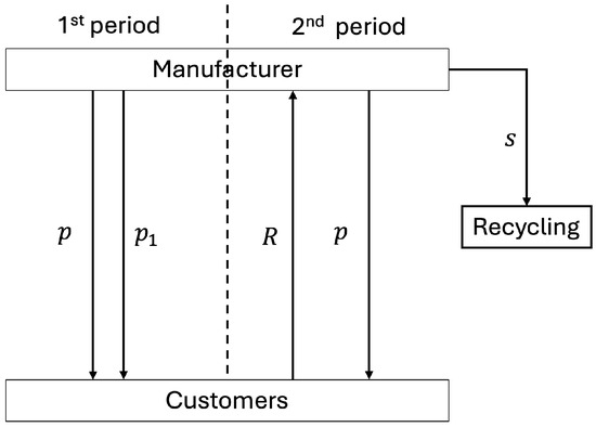
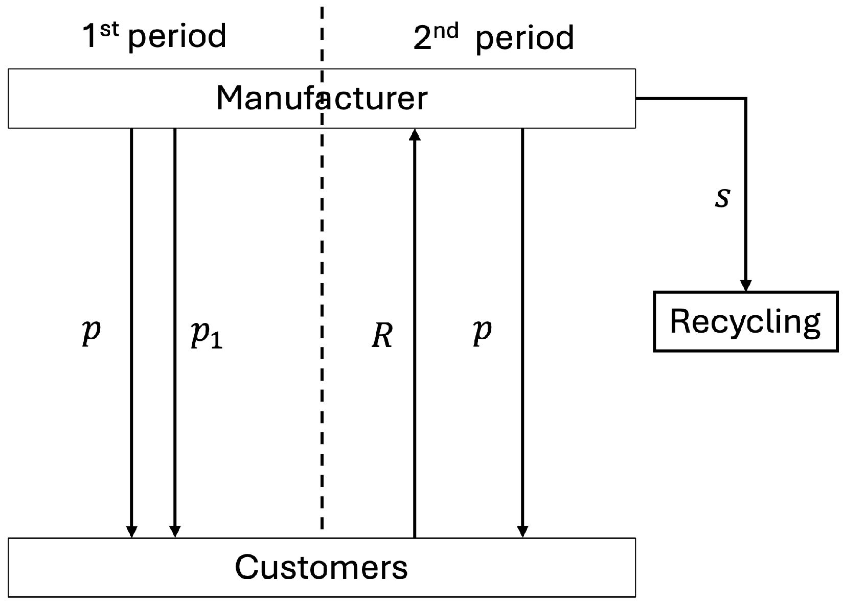
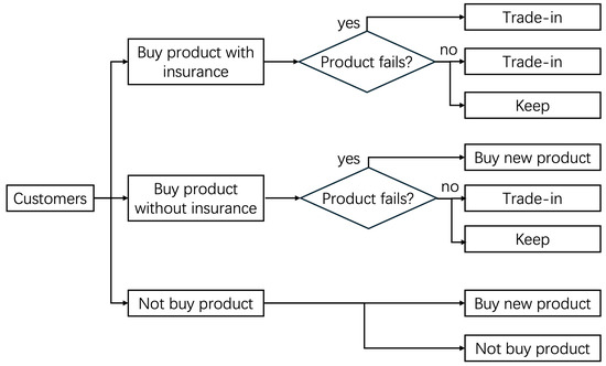
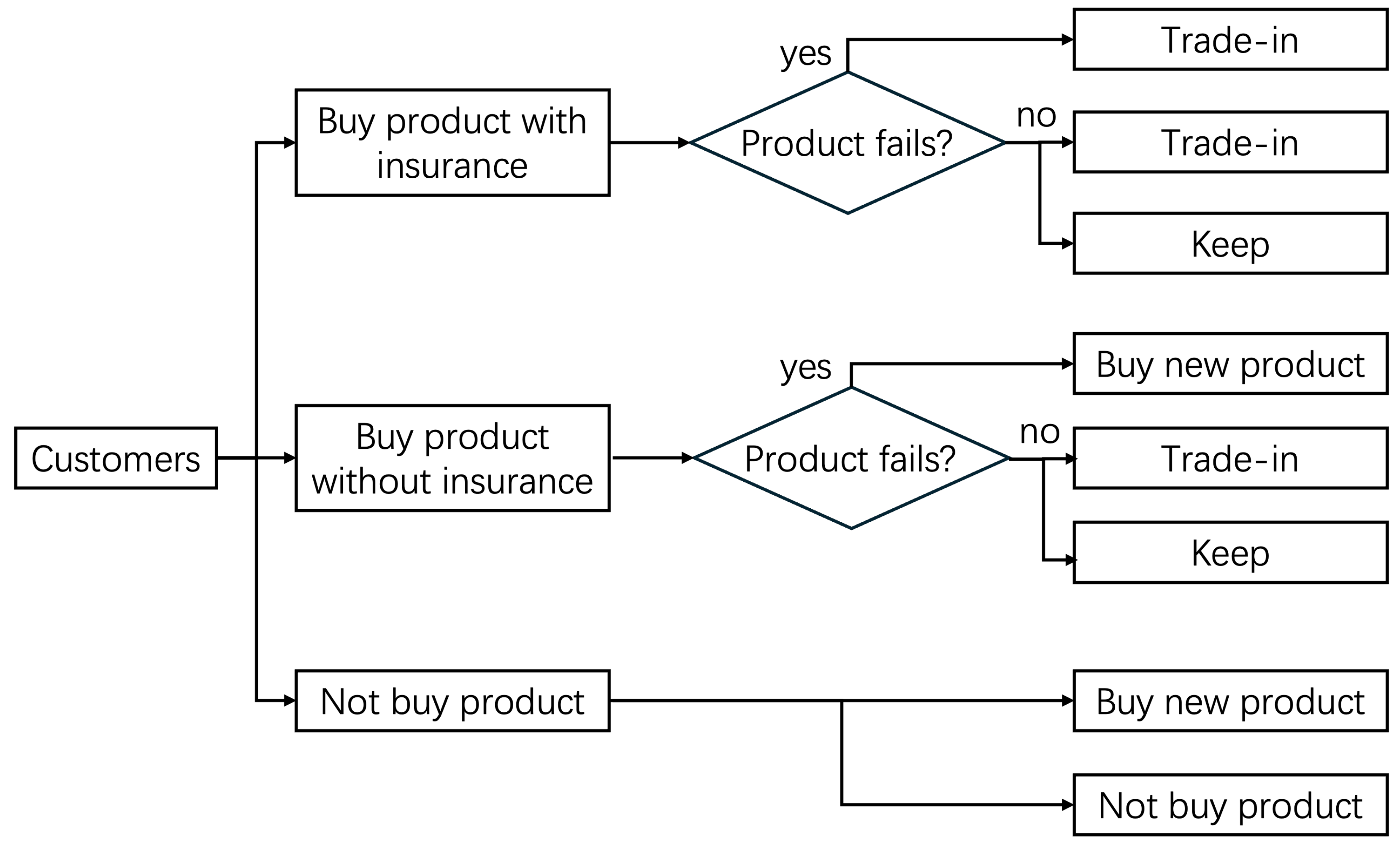
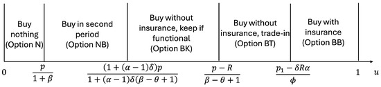
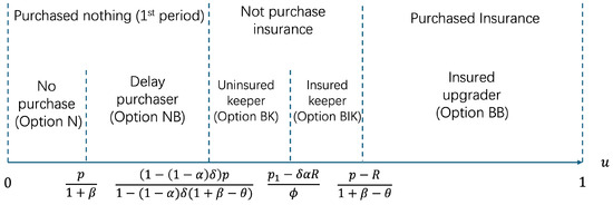
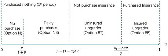
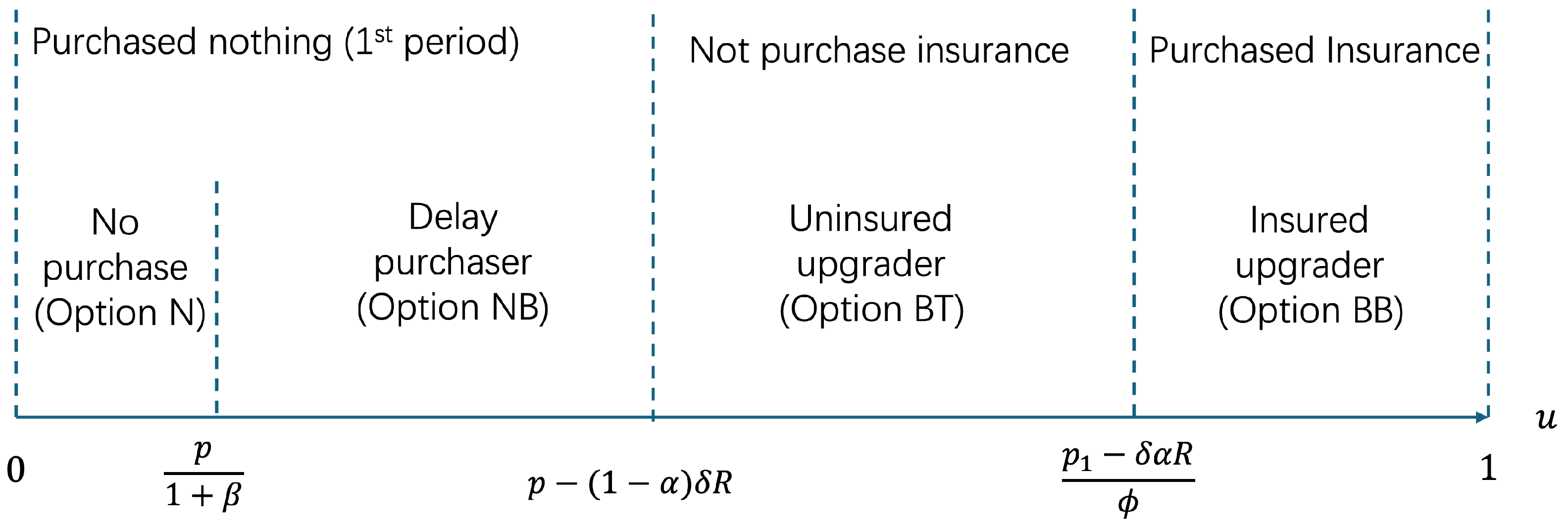
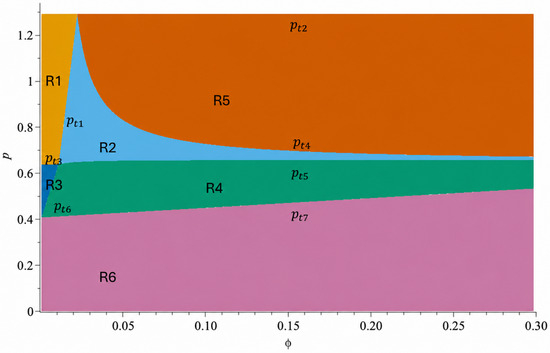
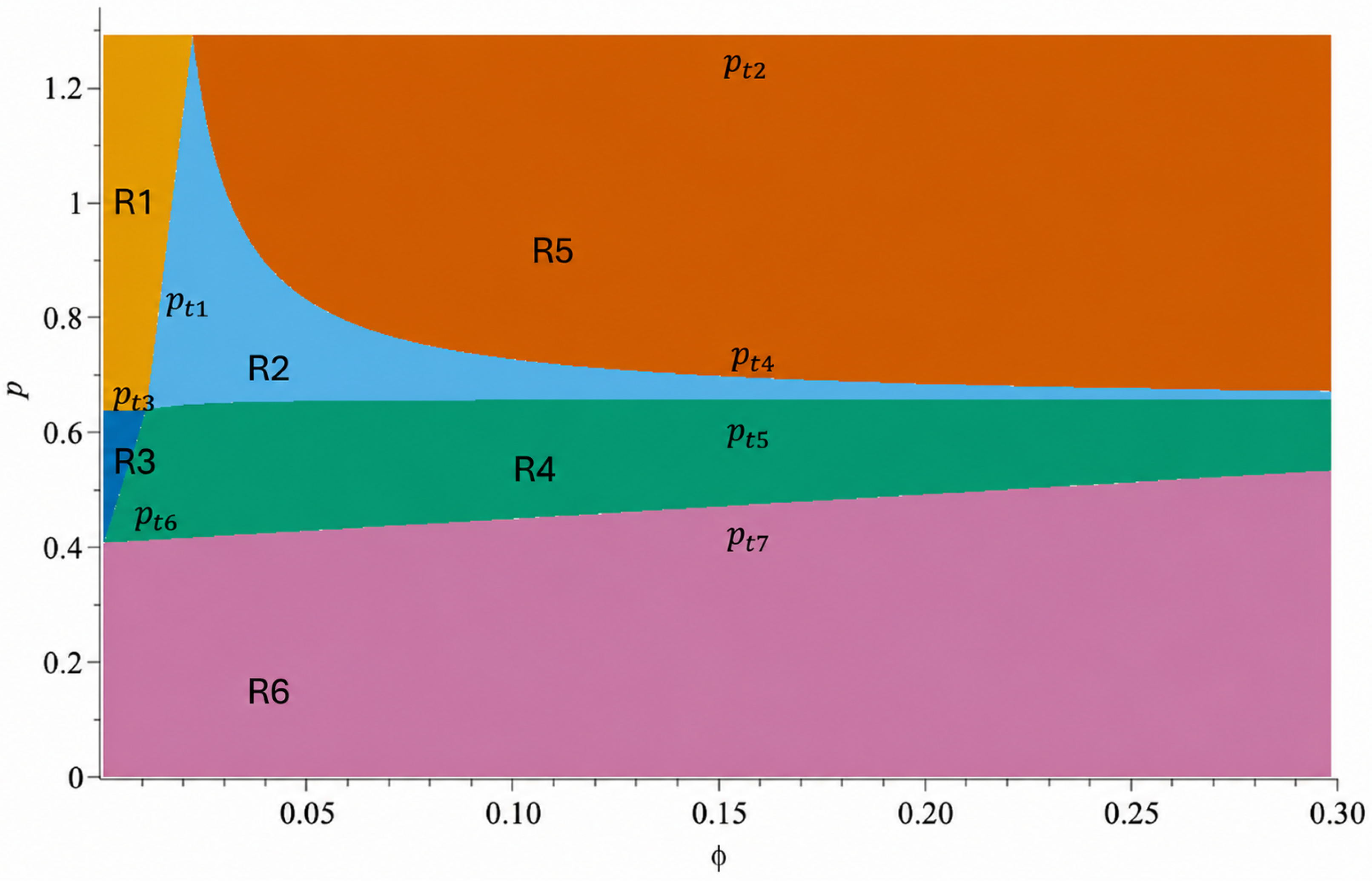
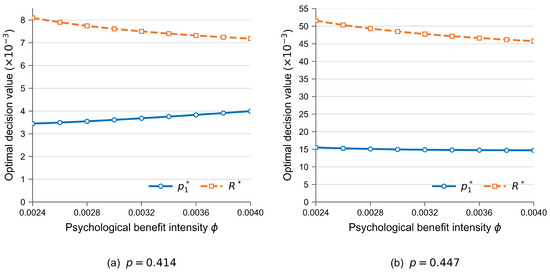
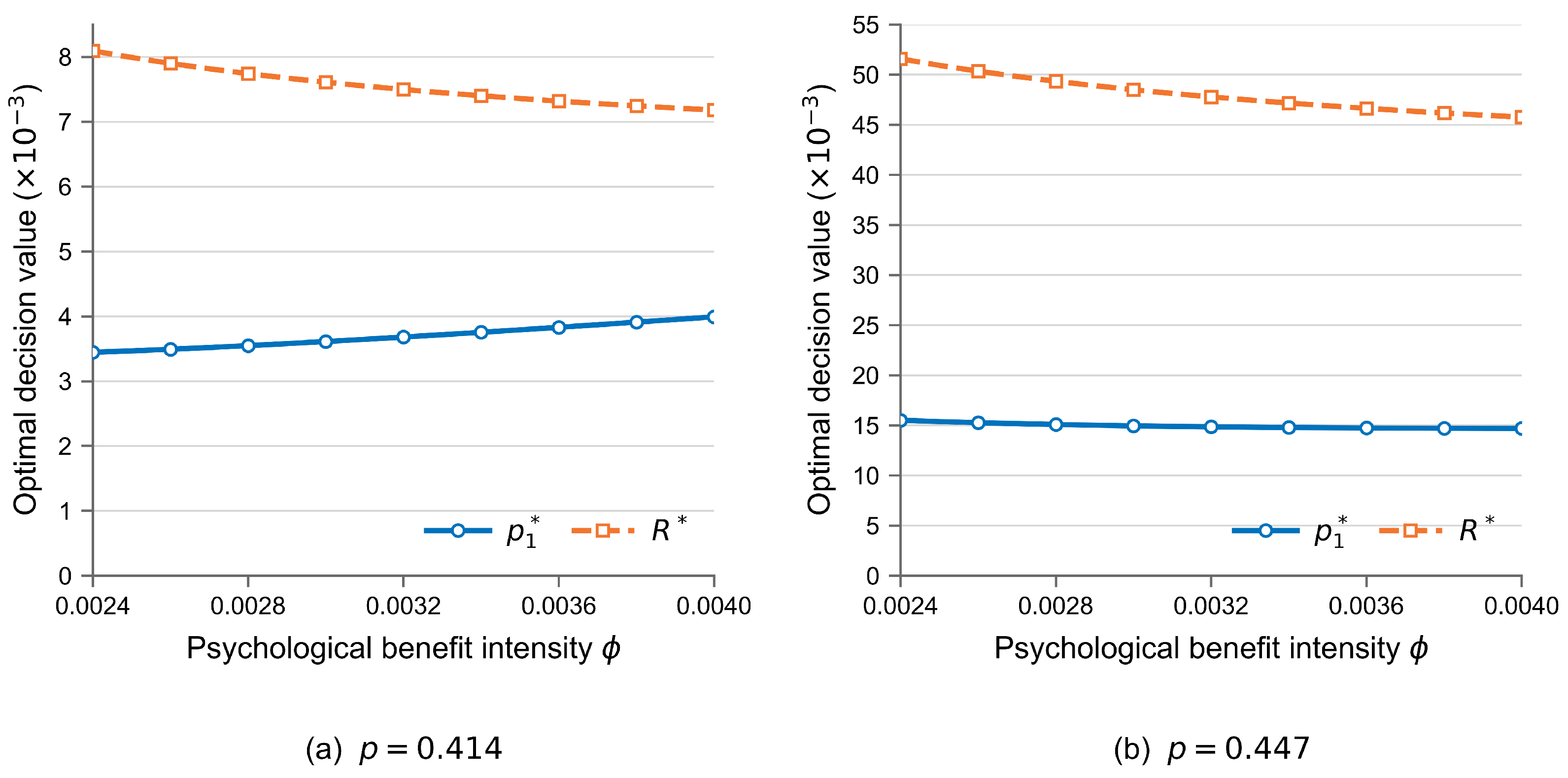
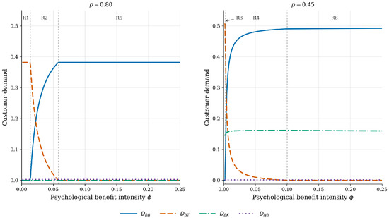
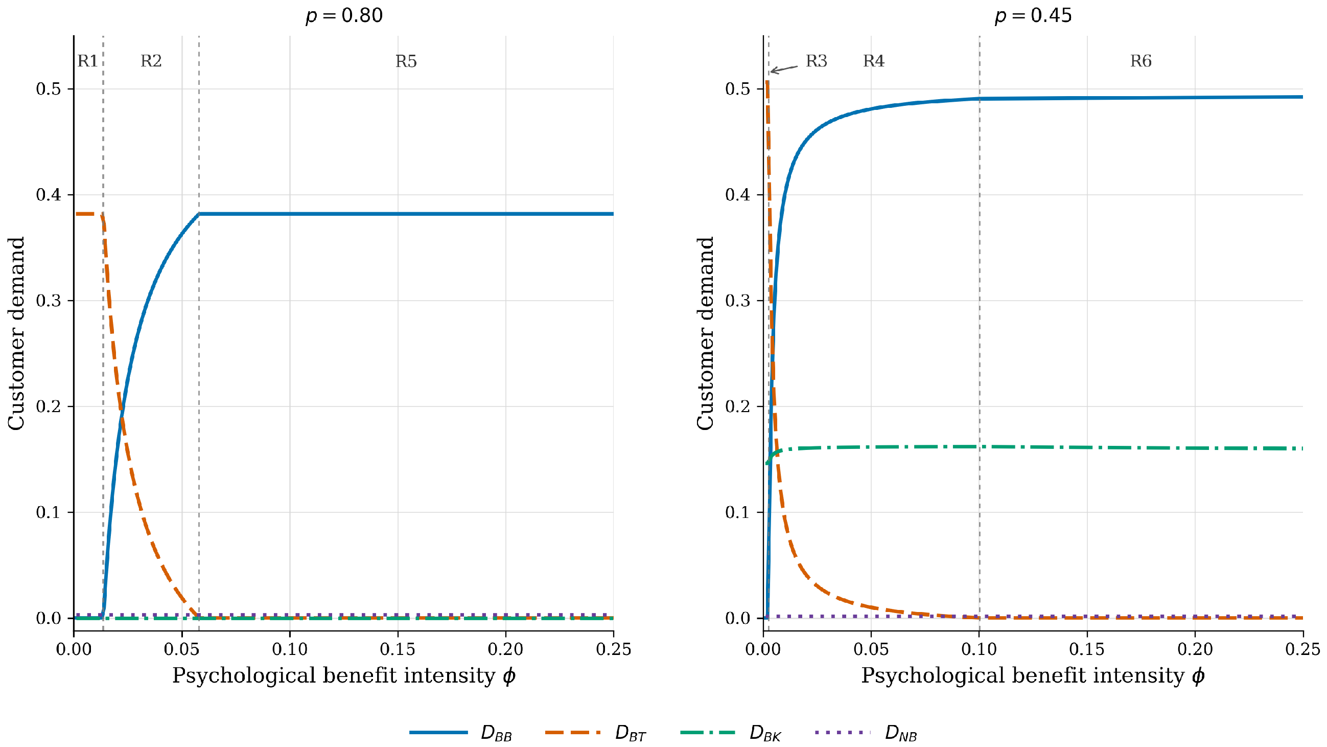
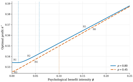
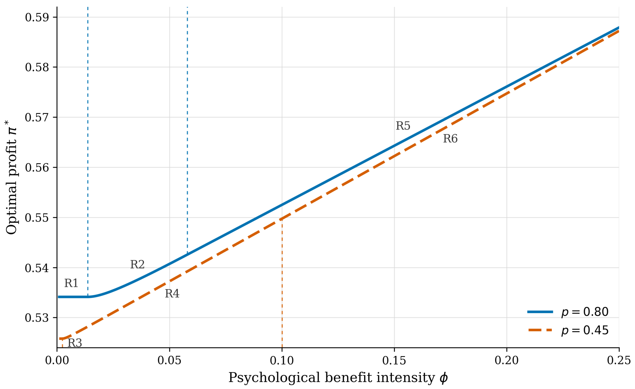
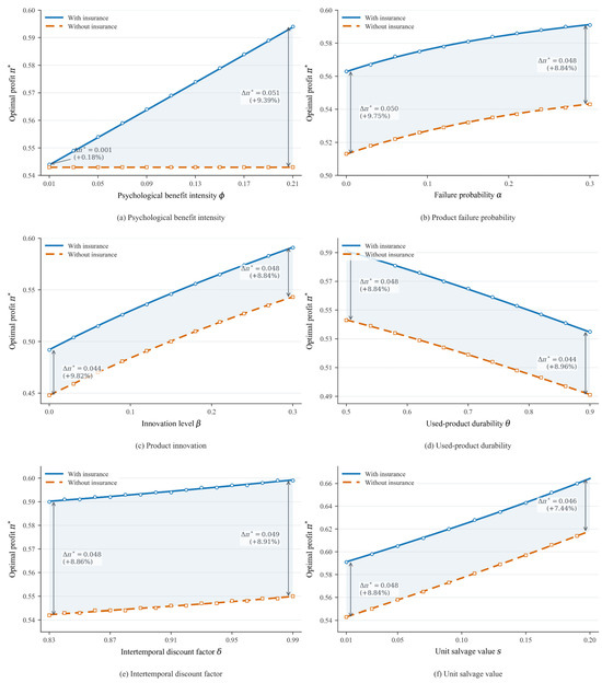
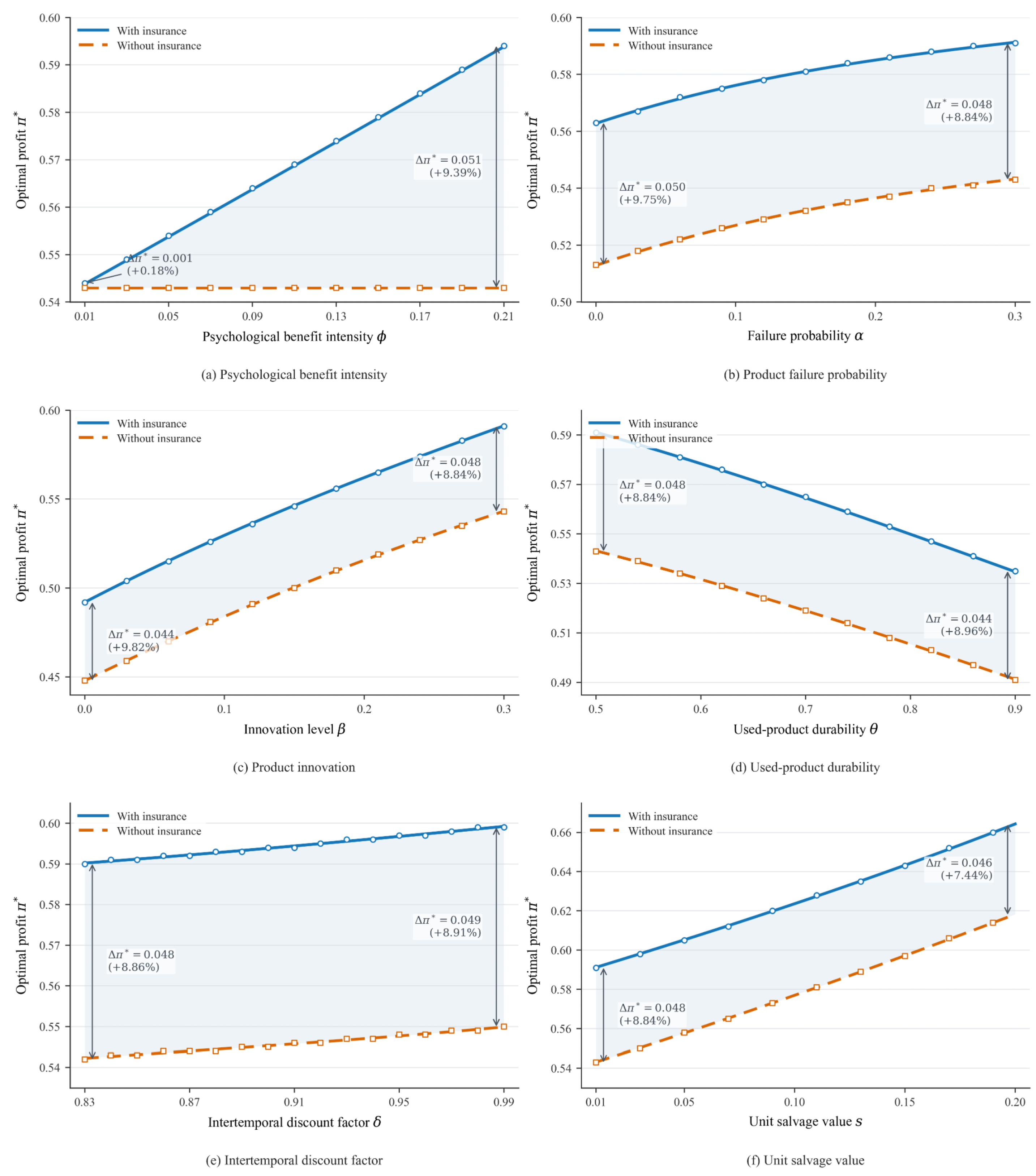

Disclaimer/Publisher’s Note: The statements, opinions and data contained in all publications are solely those of the individual author(s) and contributor(s) and not of MDPI and/or the editor(s). MDPI and/or the editor(s) disclaim responsibility for any injury to people or property resulting from any ideas, methods, instructions or products referred to in the content. |
© 2026 by the author. Licensee MDPI, Basel, Switzerland. This article is an open access article distributed under the terms and conditions of the Creative Commons Attribution (CC BY) license.