Research on Route Selection of Guangxi Cross-Border Container Multimodal Transportation Based on Mixed Time Windows

Abstract

To address the multi-objective conflicts among cost, time, and carbon emissions in Guangxi cross-border container multimodal transport—under the influence of factors such as tariffs, fluctuating customs clearance efficiency, and carbon emission policies—this paper develops a multi-objective optimization model that integrates mixed time windows and scenario analysis. The model incorporates multiple elements, including transportation cost, transshipment cost, tariff cost, time value of cargo, carbon tax cost, in-transit and customs clearance time, and transshipment-related carbon emissions, making it more aligned with real-world cross-border operational scenarios. To effectively solve this complex model, an improved NSGA-II algorithm (I-NSGA2) is designed, which introduces an adaptive crossover and mutation operator along with an elite retention strategy to enhance convergence speed and solution diversity, while embedding a scenario parameter response mechanism to accommodate dynamic fluctuations in key parameters. Subsequently, an evaluation framework is constructed using the entropy weight–TOPSIS method to select recommended routes with favorable cost–time–carbon trade-offs from the Pareto frontier. A case study based on the Nanning–Kuala Lumpur route is conducted for validation. Experimental results demonstrate that the I-NSGA2 algorithm significantly outperforms MOPSO, MOEAD, and the standard NSGA-II in terms of IGD and HV metrics; time-sensitive cargo tends to favor rail-dominated routes, while low-cost cargo prefers combined road–water–rail routes. This study effectively addresses the route selection problem for Guangxi cross-border container multimodal transport under varying key parameters, and also provides a research foundation for optimizing cross-border multimodal transport route selection in other regions.

1. Introduction

1.1. Background

The continued implementation of the Belt and Road Initiative and the Regional Comprehensive Economic Partnership (RCEP) has further deepened economic and trade cooperation between China and ASEAN. Against this background, regional trade flows have expanded steadily, creating growing demand for efficient cross-border logistics services. As a core hub of the New International Land–Sea Trade Corridor and a key gateway for China–ASEAN connectivity, Guangxi has gradually developed a cross-border containerized multimodal transport system supported by Beibu Gulf ports, land border crossings such as Pingxiang, China–Vietnam railway links, and freight services along the New International Land–Sea Trade Corridor (ILSTC). This system integrates road, rail, and waterway transport and plays an important role in linking Southwest China with ASEAN markets.

Policy initiatives issued by the General Office of the State Council, including the Work Plan for Promoting the Development of Multimodal Transport and Optimizing the Transport Structure (2021–2025), have emphasized the development of containerized multimodal transport and the transition toward greener, more efficient, and more integrated freight transport systems. These policy directions provide strategic support for the high-quality development of cross-border multimodal transport in Guangxi.

However, with the rapid expansion in trade volume and the increasing complexity of transport networks, Guangxi’s cross-border containerized multimodal transport system faces substantial operational uncertainty and multi-objective decision-making challenges. On the one hand, cross-border transport involves customs supervision, tariff policies, customs-clearance procedures, and inspection and quarantine requirements across multiple countries. Fluctuations in customs-clearance time and adjustments to tariff rates may significantly affect transportation efficiency and total logistics cost. On the other hand, internal operational constraints, such as insufficient handling capacity at transport nodes and inadequate schedule coordination, further complicate route optimization decisions. Compared with established logistics regions such as the Yangtze River Delta and the Pearl River Delta, these constraints may weaken Guangxi’s competitiveness in cross-border container transport. Therefore, it is necessary to develop route optimization methods that can jointly account for cost efficiency, delivery reliability, and operational uncertainty in multimodal transport networks.

1.2. Literature Review

In recent years, scholars both in China and abroad have conducted extensive research on the optimization of multimodal transport routes, achieving significant results in areas such as theoretical model formulation, uncertainty representation, and the application of intelligent algorithms. In terms of model formulation, early studies were mostly developed under deterministic assumptions and focused primarily on cost-based or time-based objectives, commonly using linear programming, integer programming, or mixed-integer programming models. For example, Guo et al. [1] developed a mixed-integer programming model to coordinate multi-period procurement and multimodal transport decisions by considering procurement, transportation, transshipment, and warehousing costs, with the objective of minimizing the total operating cost of cross-border e-commerce enterprises. Similarly, Somsai et al. [2] formulated three general linear programming models for multimodal distribution networks: Model I evaluates carbon emissions; Model II incorporates both carbon emissions and capacity constraints; and Model III considers total logistics costs, including transportation, handling, storage, fuel, and carbon-related costs.

With the increasing complexity of transport demand, single-objective models have become increasingly inadequate for supporting practical decision-making. Accordingly, recent studies have increasingly adopted multi-objective formulations to balance economic efficiency, delivery time, environmental performance, and operational risk. Han et al. [3] proposed a multi-objective mixed-integer linear programming model for multimodal transport of hazardous materials. Zhou et al. [4] examined the determinants of route choice in China–Europe containerized multimodal transport and developed a multi-objective optimization model considering transportation cost, transit time, and carbon emissions. Similarly, Chen et al. [5] constructed a multimodal transport network design model that jointly optimized transportation time, cargo loss risk, and carbon emissions. More recently, Hamdan et al. [6] further incorporated demand variation, fuel price fluctuations, geopolitical changes, and environmental factors into maritime route evaluation, thereby extending route optimization from deterministic cost minimization to a broader decision framework involving feasibility, economic performance, and operational constraints.

In terms of uncertainty representation in multimodal transport systems, to better reflect real-world operating conditions, scholars have introduced uncertainty decision-making approaches. Zhang et al. [7] proposed a hybrid robust stochastic optimization model for low-carbon multimodal transport route optimization and analyzed the effects of demand and time uncertainty on route decisions. Zhou et al. [8] developed a hybrid multi-criteria decision-making framework combining the Bayesian Best–Worst Method and the MARCOS method to analyze the competitive relationships among the Northern Sea Route, the Suez Canal Route, and the China Railway Express within the China–Europe multimodal transport network under the Belt and Road Initiative framework. Lv [9] investigated the optimization of railway container transport schemes in the context of the Belt and Road Initiative, focusing on the minimization of transport costs and time. Chen et al. [10] constructed a multi-level framework integrating port decisions with liner schedule design to evaluate the equilibrium accessibility of import and export containers in hub-and-spoke transport networks within the context of the ILSTC. Chen et al. [11] considered the constraints and effects of carbon taxes on carbon emissions. Taking front-end warehouse cold chain logistics as the subject, they constructed a time-dependent green vehicle routing problem model to minimize total costs and reduce carbon emissions. Hu et al. [12] indicated that intermodal transport provides substantial benefits in diminishing energy consumption and carbon emissions in long-distance freight transport, achieving total cost minimization, including carbon emission costs, through the optimization of storage node locations. Ma et al. [13] considered the uncertainty in cross-border multimodal transport demand caused by factors such as the global economic situation, trade policies between countries, and the global pandemic, and investigated strategies to reduce total costs and improve network performance.

In the field of optimization algorithm research, most studies have increasingly adopted heuristic and intelligent optimization methods, while some scholars have employed exact algorithms such as dynamic programming. Chen et al. [14] developed an optimization model for decision-making on low-carbon multimodal transport routes to address differences in cargo value and timeliness, as well as demand uncertainty, and solved it using a disaster-adaptive genetic algorithm based on Monte Carlo sampling. Ge et al. [15] used a BP neural network to forecast transportation demand for the iron ore transportation system in central China, and then employed a non-dominance sorting genetic algorithm with elite strategy to optimize multimodal transportation routes, thereby minimizing transportation costs while satisfying time-window constraints. Gao et al. [16] proposed a dynamic allocation route optimization model based on smart logistics technologies and used an improved genetic algorithm to optimize logistics distribution routes under dynamic traffic conditions. Xia et al. [17] developed a route planning method based on an improved Monte Carlo tree search algorithm to improve the stability and accuracy of dynamic route planning. Pan et al. [18] constructed an optimization model for intelligent logistics information transmission and integrated it with a multimodal transport scheduling model to support real-time dynamic route planning in logistics distribution. He L. [19] developed a shortest-path selection model for route allocation in intelligent logistics systems and applied fuzzy constraint control to improve route optimization performance. Zhao et al. [20] proposed a large-scale multimodal transport route selection model based on real-time data, using big-data analysis to detect disruptions in international transport networks and optimize transport schemes through dynamic route adjustment. Bei et al. [21] addressed perishable-goods multimodal transport by developing a multi-objective optimization model that minimizes quality loss, transportation cost, and carbon emissions while considering customer satisfaction, and solved the model using a multi-objective particle swarm optimization algorithm.

Cross-border multimodal transportation differs from domestic multimodal routing because route performance is not determined solely by transport distance, freight rate, and transshipment efficiency, but is also shaped by institutional and procedural frictions at borders. Previous studies have shown that border waiting times can be translated into freight cost changes and can generate broader trade and macroeconomic impacts [22]. Customs process innovation, such as fast-corridor arrangements, has also been shown to reduce port-related procedural burdens and improve supply-chain competitiveness by lowering time and cost frictions in international logistics nodes [23]. Recent studies further indicate that border crossing delays can be measured and estimated using multi-source operational data, including direct delay-cost estimation tools, connected-vehicle data, and Bluetooth-based border crossing datasets [24,25,26]. These findings suggest that customs clearance time, border delay, and tariff-related costs should be treated as important decision factors in cross-border route optimization rather than as external background conditions.

Delivery-time reliability is another key issue in multimodal transport route choice. In container multimodal transportation, different cargoes may have heterogeneous time sensitivity, and mixed time-window constraints can be used to distinguish between strict service requirements and acceptable delivery flexibility [27]. Related studies have described mixed time windows as a combination of hard time windows associated with scheduled transport services and soft time windows associated with consignee-side delivery flexibility [28]. In international multimodal transportation, delays in maritime or rail segments may further cause connection delays, thereby increasing the uncertainty of total transit time [29]. Soft time-window modeling has therefore been introduced into international intermodal route choice to capture the penalty effects of early or late arrivals [30]. These studies provide the methodological basis for introducing a hybrid time-window structure in the present model.

Low-carbon policy instruments have also become increasingly important in multimodal freight routing. Green intermodal service network design studies have incorporated cost, time, greenhouse-gas emissions, demand uncertainty, and travel-time uncertainty into integrated routing and service planning models [31]. In the Belt and Road context, transport service selection and routing have been analyzed by jointly considering transportation costs, in-transit inventory costs, and carbon emissions [32]. Emission limits and emission allocation schemes have further been used to represent shipper-side environmental requirements in intermodal freight transportation [33]. At the network level, multimodal logistics strategies with explicit carbon emission caps and carbon-price scenarios demonstrate that carbon regulation may induce a modal shift from road transport toward rail and waterway transport [34,35]. These studies support the inclusion of carbon emissions and carbon tax costs as core components of the multi-objective model.

Overall, existing studies have provided useful foundations for multimodal route optimization, uncertainty representation, time-window modeling, low-carbon routing, and intelligent algorithm design. However, three limitations remain. First, customs clearance, tariff-related costs, and border-delay factors are often discussed separately from route optimization models, although they are central to cross-border freight operations. Second, mixed time-window constraints have been introduced in multimodal routing, but they are rarely combined with cross-border institutional frictions and carbon-pricing mechanisms. Third, low-carbon multimodal transport studies have mainly focused on general networks, while corridor-specific evidence for the Guangxi–ASEAN containerized multimodal transport scenario remains limited. To address these gaps, this study focuses on the cross-border container multimodal transport scenario along the Guangxi–ASEAN route and develops a multi-objective route optimization model that integrates tariffs, customs clearance time, carbon taxes, and hybrid time windows.

2. Route Optimization Model for Cross-Border Containerized Multimodal Transport

The route optimization problem for Guangxi cross-border containerized multimodal transport under hybrid time windows can be described as follows. Within a specified time frame, a shipment with a known volume is required to be transported from a location in Guangxi to a designated destination in Southeast Asia. The goods may be carried by road, rail, or water from the point of origin, and the selected route may involve one or more transshipment nodes where transport modes are converted. A complete multimodal transport route is therefore determined jointly by the sequence of transport nodes and the transport mode selected for each arc.

2.1. Model Assumptions and Parameter Definitions

2.1.1. Model Assumptions

(1) The items in this shipment are all of the same kind and are all transported in standard 20-foot international containers.

(2) The shipment from the origin to the destination is treated as a single indivisible transport task, and shipment splitting is not allowed during transit.

(3) Transshipment cost and transshipment time refer to the monetary cost and operational time incurred by container handling and mode conversion at transshipment nodes. The unit transshipment cost is assumed to depend only on the pair of transport modes involved in the conversion.

(4) The total container volume processed at each transshipment node or port node must not exceed its corresponding handling capacity.

(5) At each node, mode conversion can occur at most once, and each node can be visited at most once, thereby avoiding cyclic routes.

(6) For each transport mode, the transport speed, unit freight rate, and unit carbon emission factor are assumed to be constant.

(7) The effects of force majeure events, such as extreme weather or major disruptions, on transport cost and transit time are not considered.

(8) All candidate nodes, transport arcs, and available transport modes in the cross-border containerized multimodal transport network are known in advance.

2.1.2. Notation and Parameter Definitions

The descriptions of all parameter symbols are shown in Table 1.

Table 1. Parameter descriptions.

Symbol	Description
$O;D$	Origin nodes and Destination nodes;
$A$	Set of transportation arcs, where arc $\left(i,j\right)\in A;$
$s;S$	Transport mode and set of transport modes, where $s\in S;$ $s=1,2,3$ denote road, rail, and waterway transport, respectively, and $s_1$ and $s_2$ denote two different transport modes;
$N$	Set of intermediate nodes excluding the origin $O$ and destination $D$ where $i,j\in N;$
$r;R$	A feasible route from the origin to the destination, and the set of all feasible routes;
$C$	Total transport cost of the shipment;
$T$	Total transit time of the shipment;
$E$	Total carbon emissions generated during shipment transport;
$c_i^{s_1{s}_2}$	Transshipment cost incurred when the shipment is transferred from mode $s_1$ to mode $s_2$ at node $i$;
$c_{ij}^s$	Transport cost of using mode $s$ on arc $\left(i,j\right);$
$c_{time}$	Cargo time value cost;
$t_i^{s_1{s}_2}$	Unit transshipment time incurred when the shipment is transferred from mode $s_1$ to mode $s_2$ at node $i$;
$t_{ij}^s$	Unit transit time of using mode $s$ on arc $\left(i,j\right);$
$e_i^{s_1{s}_2}$	Unit carbon emissions generated when the shipment is transferred from mode $s_1$ to mode $s_2$ at node $i$;
$e_{ij}^s$	Unit carbon emissions generated by using mode $s$ on arc $\left(i,j\right);$
$E$	Earliest allowable arrival time at the destination specified by the shipper;
$L$	Latest allowable arrival time at the destination specified by the shipper;
$[e,l]$	Preferred arrival time window at the destination specified by the shipper;
$\mathsf{\Psi }$	Unit cargo time value coefficient;
$q$	Total shipment volume, measured in TEUs; all containers are assumed to be standard 20-foot ISO containers;
$\alpha$	Early-arrival storage cost coefficient;
$\beta$	Late-arrival penalty cost coefficient;
$d_{ij}^s$	Transport distance of using mode $s$ on arc $\left(i,j\right);$;
$v^s$	Travel speed of transport mode $s$;
$ca{p}_i$	Maximum handling capacity of node $i$, measured in TEUs;
$x_{ij}^s$	Binary variable equal to 1 if the shipment is transported from node to node $j$ by mode $s$, and 0 otherwise.
$y_i^{s_1{s}_2}$	Binary variable equal to 1 if the shipment is transferred from mode $s_1$ to mode $s_2$ at node $i$, and 0 otherwise.

2.2. Analysis of Cost, Time, and Emission Components in Cross-Border Containerized Multimodal Transport

2.2.1. Cost Components of Containerized Multimodal Transport

The total cost of each cross-border containerized multimodal transport route consists of in-transit freight cost, transshipment cost, time-window penalty cost, cargo time value cost, and carbon emission cost.

(1)

In-transit freight cost under different transport modes

According to the Charging Rules for Domestic Container Road Transport, the cost of road container transport generally includes vehicle operating cost, vehicle depreciation, and insurance expenses. Taking containers as the basic accounting unit, the freight cost of road transport consists of two components: the basic freight charge and the container trip charge. The basic freight charge refers to the cost charged per unit transport distance for a container, calculated as the product of the unit container freight rate, the number of containers, and the transport mileage. The container trip charge varies according to container size, and the total container trip charge is obtained by multiplying the per-container trip charge by the number of containers. The in-transit freight cost of road container transport is formulated in Equation (1).

For rail container transport, the freight cost is calculated according to the standardized pricing system specified in the Railway Freight Tariff Rules. Specifically, the railway transport cost is determined by the base tariff and transport mileage, as shown in Equation (2).

For waterway container transport, three pricing methods are commonly used: the box-rate method, the navigation-zone tariff method, and the uniform tariff method. Since this study involves seaborne container transport, the box-rate method is adopted to calculate maritime freight cost, as expressed in Equation (3).

$$c_{ij}^{s=1}=c^h\times d_{ij}^{s=1}\times q+c^{x}q$$

(1)

where $c^h$ is the unit freight rate for road container transport, expressed in CNY/(container·km), and $c^x$ is the fixed trip charge per 20-foot container for road transport, expressed in CNY/container.

$$c_{ij}^{s=2}=(c^r\times d_{ij}^{s=2}+C_x)\times q$$

(2)

where $c^r$ denotes the operating base tariff for rail container transport, expressed in CNY/(container·km), and $C_x$ denotes the departure base tariff for rail container transport, expressed in CNY/container.

$$c_{ij}^{s=3}=c^w\times d_{ij}^{s=3}\times q$$

(3)

where $c^w$ denotes the maritime freight rate, expressed in CNY/container.

(2)

Container Transshipment Cost at Nodes

When containers are transferred between transport modes at a node, costs are incurred for loading and unloading, temporary storage, short-distance yard handling, and additional management services. Since different mode conversions involve different operational procedures at transshipment nodes, the corresponding transshipment cost may vary across transport-mode pairs. For example, transshipment between road and rail generally involves loading and unloading, mode conversion, and management-related costs, whereas transshipment between rail and waterway transport may involve costs such as berthing, vessel dispatching, and port surcharges. In addition, shipments transported on cross-border arcs are subject to customs clearance and inspection procedures, which generate customs-related service costs. Therefore, the transshipment cost is formulated in Equation (4).

$$\begin{array}{l}{c}_i^{s_1{s}_2}=c_i\times q+C_{tariff}\\ C_{tariff}=L_{ij}q\end{array}$$

(4)

where $c_i$ denotes the unit transshipment cost per container; $L_{ij}$ denotes the tariff rate applied when arc $(i,j)$ crosses a customs boundary.

(3)

Time-window penalty cost for early or late arrivals

In actual freight transport, the arrival time of a shipment at the destination may deviate from the delivery time expected by the shipper due to various uncertain factors. To capture this deviation, a hybrid time-window structure at the destination is introduced. Under this setting, a shipment that arrives outside the preferred delivery-time window but within the allowable relaxed time window is still accepted, although an early or late arrival incurs a penalty cost. Early arrival may generate waiting and temporary storage costs when the consignee has insufficient warehousing capacity, whereas late arrival may affect cargo quality or disrupt downstream operations, resulting in higher penalty costs. The unit penalty cost incurred when the shipment fails to arrive within the preferred delivery-time window is given in Equation (5).

$$p^M(T)=\left\{\begin{array}{l}M,0\le t<E,\\ \alpha (e-t),E\le t<e,\\ 0,e\le t\le l,\\ \beta (t-l),l<t\le L,\\ M,L<t,\end{array}\right.$$

(5)

(4)

Cargo time value cost

In multimodal route optimization, transport time generates not only transportation and transshipment costs but also implicit time-related and capital-occupation costs. A longer in-transit time increases implicit losses associated with capital tied up in cargo, inventory delay, and delayed market delivery. Therefore, this cost should be quantified in the optimization model to capture the effect of transit time on the time value of cargo. Let $V$ denote the cargo value per container and $\rho$ denote the annual cargo holding-cost coefficient. The unit-time capital-occupation cost is then calculated as shown in Equation (6). The value of $\rho$ varies across cargo categories.

$$c_{time}={\displaystyle \frac{V\cdot q\cdot \rho \cdot T}{365\times 24}}$$

(6)

2.2.2. Time Components of Containerized Multimodal Transport

The time involved in container multimodal transport consists of container in-transit travel time and node operation time. The in-transit travel time of containers is determined by the transport distance and the speed parameters of the selected transport mode. In the model, node operation time, along with transshipment handling time and customs clearance time, is uniformly incorporated into the calculation of total route time. The transshipment handling time parameter is used to capture the differences in connection efficiency among alternative schemes, thereby providing a foundation for the subsequent formulation of time-window constraints and the quantification of cargo time value cost.

2.2.3. Carbon Emission Components of Containerized Multimodal Transport

Since containerized multimodal transport is generally organized on a per-container basis, carbon emissions are often converted from ton-kilometers to TEU-kilometers or measured as total emissions per container over the entire route. From a whole-chain perspective, emissions should be calculated separately for transport segments and logistics nodes. Transport segments include road feeder links, rail trunk lines, inland waterway links, and maritime shipping routes, whereas logistics nodes include loading and unloading, temporary storage, transshipment, and container repositioning operations at seaports and inland ports. In the context of Guangxi cross-border containerized multimodal transport, carbon emissions are mainly generated by inter-node transportation and transshipment operations.

(1)

Carbon emissions generated during container transport

Carbon emissions from transport activities can be calculated using the emission factor of each transport mode, as shown in Equation (7). The emission factor $E{F}^s$ for each transport mode is obtained from official data released by the Ministry of Transport of China. Since the units of the originally reported values are not consistent with the per-container emission factors used in this study, unit conversion based on the weight of each container is required in subsequent calculations.

$$e_{ij}^s=q\cdot d_{ij}^s\cdot E{F}^s$$

(7)

where $E{F}^s$ denotes the carbon emission factor of transport mode per container, with the unit of g CO₂ per ton per kilometer.

(2)

Carbon emissions from container transshipment and handling

In containerized multimodal transport, containers undergo loading, unloading, temporary storage, transshipment, and other handling operations at logistics nodes, all of which consume energy and generate carbon emissions. Due to differences in transshipment distance, transshipment volume, and operational procedures, the carbon emissions associated with inter-modal transshipment vary across mode-conversion pairs. The carbon emissions from node-based transshipment operations are mainly determined by the transshipment volume and the specific mode-conversion pair. In this study, the emission coefficient associated with each transport-mode conversion is treated as a fixed relative emission coefficient. The carbon emissions generated during transshipment are calculated as shown in Equation (8).

$$e_i^{s_1{s}_2}=q\cdot E{F}_i^{s_1{s}_2}$$

(8)

where $E{F}_i^{s_1{s}_2}$ denotes the carbon emissions generated by a single container when the shipment is transferred from transport mode $s_1$ to transport mode $s_2$ at node $i$.

In addition, a carbon tax mechanism is introduced to monetize the carbon emissions generated during Guangxi cross-border containerized multimodal transport. The carbon tax level should balance environmental benefits and economic feasibility. Referring to relevant research data released by the Ministry of Ecology and Environment of China, the carbon tax rate is set at USD 20 per ton of CO₂. The carbon tax calculation is shown in Equation (9). Based on this setting, the carbon emission cost is obtained by multiplying the total carbon emissions by the carbon tax rate. The carbon emission cost incurred when the shipment is transported from node $i$ to node $j$ by mode $s$ is calculated as shown in Equation (10).

$$\sigma ={\displaystyle \sum _0^t{D}_t}{(1+\lambda )}^{-t}$$

(9)

where $D_t$ denotes the damage cost per unit of carbon emissions in year $t$, and $\lambda$ denotes the discount rate.

$$c_e=\theta \cdot (e_{ij}^s+e_i^{s1s2})$$

(10)

2.3. Model Solution

The multimodal transport network is represented as $G=(N,A,S)$, where $N$ is the set of all network nodes, $A$ denotes the set of transport arcs, and $S$ denotes the set of available transport modes. Consider a containerized shipment with volume $q$ transported from the origin $O$ to the destination $D$. The shipment departs at time $t_0$ and is required to arrive within the prescribed delivery-time window $\left[E,L\right]$. Based on the route optimization problem for cross-border containerized multimodal transport, a multi-objective programming model is formulated with three objectives: cost, time, and carbon emissions.

(1)

Total transport cost

Weight parameters are introduced to reflect the relative contributions of different cost components to the total cost: let $w_1$ be the weight of costs such as in-transit transportation cost, node transshipment cost, penalty cost, carbon tax, and other expenses in the total cost; let $w_2$ be the weight of cargo time value cost in the total cost. The objective function for minimizing the total transportation cost $C$ is derived as shown in Equation (11).

$$\min C=w_1\left({\displaystyle {\displaystyle \sum _{(i,j)\in A}}{\displaystyle \sum _{s\in S}{c}_{ij}^s}}{x}_{ij}^s+{\displaystyle {\displaystyle \sum _{i\in N}}{\displaystyle \sum _{s_1\in S}{\displaystyle \sum _{s_2\in S,s_2\ne s_1}{c}_i^{s_1{s}_2}{y}_i^{s_1{s}_2}}+p(T)\cdot q}}+\theta \cdot e_{ij}^s\right)+w_2{c}_{time}$$

(11)

(2)

Total transit time

Transportation time mainly includes container in-transit travel time and node operation time, with customs clearance time and transshipment handling time included in the node operation time. The objective function for minimizing the total transportation time $T$ is shown in the following Equation (12).

$$\min T={\displaystyle {\displaystyle \sum _{(i,j)\in A}}{\displaystyle \sum _{s\in S}{t}_{ij}^s}}{x}_{ij}^s+{\displaystyle {\displaystyle \sum _{i\in N}}{\displaystyle \sum _{s_1\ne s_2}{t}_i^{s_1{s}_2}{y}_i^{s_1{s}_2}}}$$

(12)

(3)

Total carbon emissions

The total carbon emissions generated throughout the transport process indicate the environmental performance of the selected transport modes. Therefore, minimizing transport-related carbon emissions is included as one of the optimization objectives. The corresponding objective function is formulated in Equation (13).

$$\min E={\displaystyle {\displaystyle \sum _{(i,j)\in A}}{\displaystyle \sum _{s\in S}{e}_{ij}^s{x}_{ij}^s}}+{\displaystyle {\displaystyle \sum _{i\in N}}{\displaystyle \sum _{s_1,s_2\in S}{e}_i^{s_1{s}_2}{y}_i^{s_1{s}_2}}}=q{\displaystyle {\displaystyle \sum _{(i,j)\in A}}{\displaystyle \sum _{s\in S}E{F}^s{d}_{ij}^s{x}_{ij}^s}}+q{\displaystyle {\displaystyle \sum _{i\in N}}{\displaystyle \sum _{s_1\in S}{\displaystyle \sum _{s_2\in S,s_2\ne s_1}E{F}_i{y}_i^{s_1{s}_2}}}}$$

(13)

In containerized cargo transportation, minimizing transit time generally necessitates selecting expedited modes of transport, which frequently incur elevated shipping expenses. Therefore, a typical trade-off exists between transit time and transport cost, making it difficult to minimize both objectives simultaneously. In addition, carbon emissions are incorporated as a further optimization objective in this study. Accordingly, a multi-objective optimization model is formulated to jointly improve economic efficiency, delivery timeliness, and environmental performance. The multi-objective function is presented in Equation (14).

$$\begin{array}{l}\min F=[C,T,E]\\ =\left[w_1\left({\displaystyle {\displaystyle \sum _{(i,j)\in A}}{\displaystyle \sum _{s\in S}{c}_{ij}^s}}{x}_{ij}^s+{\displaystyle {\displaystyle \sum _{i\in N}}{\displaystyle \sum _{s_1\in S}{\displaystyle \sum _{s_2\in S,s_2\ne s_1}{c}_i^{s_1{s}_2}{y}_i^{s_1{s}_2}}+p(T)\cdot q}}+\theta \cdot e_{ij}^s\right)+w_2{c}_{time}\right]+\\ \left({\displaystyle {\displaystyle \sum _{(i,j)\in A}}{\displaystyle \sum _{s\in S}{t}_{ij}^s}}{x}_{ij}^s+{\displaystyle {\displaystyle \sum _{i\in N}}{\displaystyle \sum _{s_1\ne s_2}{t}_i^{s_1{s}_2}{y}_i^{s_1{s}_2}}}\right)+q\left({\displaystyle {\displaystyle \sum _{(i,j)\in A}}{\displaystyle \sum _{s\in S}E{F}^s{d}_{ij}^s{x}_{ij}^s}}+{\displaystyle {\displaystyle \sum _{i\in N}}{\displaystyle \sum _{s_1\in S}{\displaystyle \sum _{s_2\in S,s_2\ne s_1}E{F}_i{y}_i^{s_1{s}_2}}}}\right)\end{array}$$

(14)

The model is subject to the following constraints:

$${\displaystyle \sum _{r\in R}{x}_r}=1$$

(15)

$${\displaystyle {\displaystyle \sum _{i,j\in N}}{\displaystyle \sum _{s\in S}{x}_{ij}^s}}+{\displaystyle {\displaystyle \sum _{i,j\in N}}{\displaystyle \sum _{s\in S}{x}_{ji}^s}}=1$$

(16)

$${\displaystyle \sum _i{\displaystyle \sum _{s_1,s_2\in S}{y}_i^{s_1,s_2}}}\le 1$$

(17)

$${\displaystyle {\displaystyle \sum _{s\in S}}{\displaystyle \sum _{(1,j)\in A}{x}_{1,j}^s}}=1;{\displaystyle {\displaystyle \sum _{s\in S}}{\displaystyle \sum _{(i,20)\in A}{x}_{i,20}^s}}=1$$

(18)

$${\displaystyle {\displaystyle \sum _{s\in S}}{\displaystyle \sum _{(k,j)\in A}{x}_{k,j}^s}}-{\displaystyle {\displaystyle \sum _{s\in S}}{\displaystyle \sum _{(i,k)\in A}{x}_{i,k}^s}}=0,\forall k\in N$$

(19)

$$q{\displaystyle \sum _{s\in S}{\displaystyle \sum _{(i,j)\in A}{x}_{ij}^s}}\le ca{p}_i,\forall i\in N$$

(20)

$$E\le T\le L$$

(21)

$${\displaystyle {\displaystyle \sum _{(j,i)\in A}}{x}_{ji}^{s_1}}+{\displaystyle {\displaystyle \sum _{(i,k)\in A}}{x}_{ik}^{s_2}-1}\le y_i^{s_1{s}_2},\forall i\in N,s_1,s_2\in S,s_1\ne s_2$$

(22)

$$y_i^{s_1{s}_2}\le {\displaystyle {\displaystyle \sum _{(j,i)\in A}}{x}_{ji}^{s_1}},y_i^{s_1{s}_2}\le {\displaystyle {\displaystyle \sum _{(i,k)\in A}}{x}_{ik}^{s_2}}$$

(23)

$$d_{ij}^s\ge 0,d_{ji}^s=0$$

(24)

$$\begin{array}{l}{x}_{ij}^s\in \left\{0,1\right\},\forall (i,j)\in A,s\in S\\ y_i^{s_1{s}_2}\in \left\{0,1\right\},\forall i\in N,s_1,s_2\in S,s_1\ne s_2\end{array}$$

(25)

Based on the above assumptions, the proposed model is subject to the constraints defined in Equations (15)–(25). Equation (15) ensures that the shipment is treated as an indivisible transport task. Equation (16) restricts each node to be visited once only, thereby avoiding cyclic routes. Equation (17) imposes the transshipment-frequency constraint, ensuring that the shipment is transferred at most once at each node. Equations (18) and (19) define path connectivity and flow conservation, ensuring that exactly one route departs from the origin $O$, exactly one route terminates at the destination $D$, and flow is conserved at all intermediate nodes. Equation (20) represents the node-capacity constraint: for each intermediate node $i\in N$, the container volume processed at node $i$ must not exceed its maximum handling capacity $ca{p}_i$. Equation (21) specifies the arrival time-window constraint. Equation (22) defines the transport-mode conversion constraint: when the shipment is transferred from mode $s_1$ to mode $s_2$ at node $i$, the corresponding transshipment variable $y_i^{s_1{s}_2}$ is activated. Equation (23) further specifies that $y_i^{s_1{s}_2}=1$ if and only if the incoming arc before node $i$ uses mode $s_1$ and the outgoing arc after node $i$ uses mode $s_2$; it also prevents return detours after the shipment departs from the origin. Equations (24) and (25) define the domains of the decision variables.

3. Improved NSGA-II Algorithm

Building on the standard NSGA-II framework, this study introduces three improvements involving population initialization, the crossover operator, and the local search mechanism. The improved algorithm retains the non-dominated sorting and crowding-distance-based environmental selection procedures of NSGA-II, while enhancing global search capability and convergence performance through improved initial sample distribution and adaptive search strategies.

3.1. Population Initialization Based on Latin Hypercube Sampling

Let the decision space be $\mathsf{\Omega }=\left\{x\in R^D\left|l_i\le x_i\le u_i,i=1,\dots ,D\right.\right\}$ and the population size be $N$. To improve the coverage of initial solutions within the decision space, Latin Hypercube Sampling (LHS) is adopted to generate the initial population. For the i-th dimension, divide the interval $\left[l_i,u_i\right]$ equally into $N$ sub-intervals with length ${\mathsf{\Delta }}_i={\displaystyle \frac{u_i-l_i}{N}}$, and denote each sub-interval as $\left[l_j+(k-1){\mathsf{\Delta }}_j,l_j+k{\mathsf{\Delta }}_j\right](k=1,2,\dots ,N)$.

Construct a random permutation ${\pi }_i=\left[{\pi }_{i1},{\pi }_{i2},\dots ,{\pi }_{iN}\right]({\pi }_{ij} \in \{1,2,\dots ,N)$ of $\left\{1,2,\dots ,N\right\}$, and perform uniform sampling within each sub-interval. Then the sampled value of the n-th individual at the i-th dimension is defined as ${\tilde{x}}_{ji}=l_i+({\pi }_{ij}+u_{ji}){\mathsf{\Delta }}_i,u_{ji}~U(0,1),j=1,\dots ,N$.

On the basis of LSH samples, zero-mean Gaussian noise is superimposed to further enhance local perturbation, followed by boundary projection operation. ${\tilde{x}}_{ji}={\tilde{x}}_{ji}+{\epsilon }_{ji},{\epsilon }_{ji}~N(0,{0.1}^2)$, $x_{ji}={\mathsf{\Pi }}_{\left[l_i,u_i\right]}({\tilde{x}}_{ji})=\min \left\{\max \left\{{\tilde{x}}_{ji},l_i\right\},u_i\right\}$.

Ensure that decision variables are constrained within the feasible range, $x_{ji}=clip(x_{ji}^1,l{b}_i,u{b}_i)=\left\{\begin{array}{l}l{b}_i,x_{ji}^1<l{b}_i\\ x_{ji}^1,l{b}_i\le x_{ji}^1<u{b}_i\\ u{b}_i,x_{ji}^1>u{b}_i\end{array}\right.$

An initial population is thus obtained, $X^{(0)}=\left\{x_1^{(0)},\dots ,x_N^{(0)}\right\},x_j^{(0)}={(x_{j1},\dots ,x_{jD})}^{\top }$.

3.2. Adaptive Simulated Binary Crossover Based on Population Density

To dynamically balance global exploration and local exploitation during the evolutionary process, an adaptive distribution index based on population diversity is introduced into the simulated binary crossover (SBX) operator. Let the population at generation t be $X^{(t)}={\left\{x_k^{(t)}\right\}}_{k=1}^N,x_k^{(t)}\in {ℝ}^D$, and assume that each dimension has been normalized to $\left[0,1\right]$; then the population center is $c^{(t)}={\displaystyle \frac{1}{N}}{\displaystyle \sum _{k=1}^N{x}_k^{(t)}}$. The Euclidean distance from the k-th individual to the center is $d_k^{(t)}={\left|\left|x_k^{(t)}-c^{(t)}\right|\right|}_2==\sqrt{{{\displaystyle \sum _{j=1}^D(x_{kj}^{(t)}-c_j^{(t)})}}^2}$.

The average distance ${\overline{d}}^{(t)}={\displaystyle \frac{1}{N}}{\displaystyle \sum _{k=1}^N{d}_k^{(t)}}$ is thus obtained. In the normalized space, the normalized diversity index is defined as $D_{iv}^{(t)}=\max \left\{0,\min \left\{1,{\displaystyle \frac{{\overline{d}}^{(t)}}{d_{\max }}}\right\}\right\}\in \left[0,1\right]$, where $d_{\max }={\displaystyle \frac{1}{2}}\sqrt{{{\displaystyle \sum _{j=1}^D(u{b}_j-l{b}_j)}}^2}$ denotes the maximum theoretical distance of the decision space.

The distribution index of SBX at the t-th generation is assigned as ${\eta }_c^{(t)}=1+9D_{iv}^{(t)},{\eta }_c^{(t)}\in \left[1,10\right]$.

In the specific crossover operation, let $x_{aj}^{(t)}=\min \left\{x_{aj}^{(t)},x_{bj}^{(t)}\right\},x_{bj}^{(t)}=\max \left\{x_{aj}^{(t)},x_{bj}^{(t)}\right\}$ represent the j-th dimension of the parent individual.

The offspring generation formula is expressed as ${\beta }_j=\left\{\begin{array}{l}{(2u_j)}^{{\displaystyle \frac{1}{{\eta }_c^{(t)}+1}}},u_j\le 0.5\\ {\left({\displaystyle \frac{1}{2(1-u_j)}}\right)}^{{\displaystyle \frac{1}{{\eta }_c^{(t)}+1}}},u_j>0.5\end{array}\right.$, where $u_j~U(0,1)$ is a uniformly distributed random number.

The final offspring decision variable is $x_{aj}^{\prime }=0.5\cdot \left[(1+{\beta }_j)x_{aj}^{(t)}+(1-{\beta }_j)x_{bj}^{(t)}\right]$, $x_{bj}^{\prime }=0.5\cdot \left[(1-{\beta }_j)x_{aj}^{(t)}+(1+{\beta }_j)x_{bj}^{(t)}\right]$.

Since ${\eta }_c^{(t)}$ is positively correlated with diversity $D_{iv}^{(t)}$, this resolves the problem that a fixed ${\eta }_c^{(t)}$ cannot adapt to the entire algorithm lifecycle. When the population is widely distributed and $D_{iv}^{(t)}$ is large, ${\eta }_c^{(t)}$ takes a higher value, and the crossover results are closer to the parents. The algorithm tends to perform fine exploitation in the current promising region. When the population tends to converge and $D_{iv}^{(t)}$ decreases, ${\eta }_c^{(t)}$ decreases accordingly, and the offspring generated by crossover are more widely distributed, thereby enhancing the global exploration ability and inhibiting premature convergence.

3.3. Bit-Flip-Based Local Neighborhood Search

To further improve the approximation accuracy of the solution set to the true Pareto front, a bit-flip-based local neighborhood search is performed on the current first non-dominated front after completing the standard NSGA-II operations in each generation.

Let the first non-dominated front obtained at generation $t$ be denoted as $F_1^{(t)}={\left\{x_j^{(t)}\right\}}_{j=1}^{N_1},x_j^{(t)}\in \mathsf{\Omega }$. The corresponding objective vectors are given by $f\left(x_j^{(t)}\right)=\left(f_1(x_j^{(t)}),\dots ,f_M(x_j^{(t)})\right)$. Since the decision variables of the model are binary in nature, the local search operation adopts a bit-flip strategy. Specifically, for each solution $x_j^{(t)}$ in the current non-dominated solution set, each bit in its encoding string is flipped with probability $p$. To balance the exploration and exploitation capabilities of the algorithm, the flip probability $p$ is dynamically adjusted with the iteration count $t$, and is calculated as follows:$p=p_{\max }-{\displaystyle \frac{(p_{\max }-p_{\min })\times t}{T_{\max }}}$, where $p_{\max }$ and $p_{\min }$ are the preset maximum and minimum flip probabilities, respectively, and $T_{\max }$ is the maximum number of iterations. For each generated neighborhood set, its objective vectors $f(x_j^{\prime (t)})$ are computed. One implementation is to adopt a greedy replacement rule, whereby a new solution replaces the original one if it is not worse than the original solution in the Pareto sense: $x_j^{(t+1)}=\left\{\begin{array}{l}{x}_j^{\prime (t)},x_j^{\prime (t)}\prec x_j^{(t)}\\ x_j^{(t)},Otherwise\end{array}\right.$, where $\prec$ denotes the Pareto dominance relation. Alternatively, all neighborhood solutions can be combined with the current population, followed by another round of non-dominated sorting and crowding-distance-based environmental selection: $X^{(t+1)}\subseteq select(X^{(t)}\cup {\left\{x_j^{\prime (t)}\right\}}_{j=1}^{N_1})$.

By incorporating the above three improvements, the I-NSGA2 algorithm is constructed on the basis of the standard NSGA-II framework while retaining its structural simplicity. The proposed algorithm enhances the spatial coverage of the initial population, improves the adaptive search capability during multi-generation evolution, and strengthens local fine-search capability for approximating the Pareto front. These improvements enable the algorithm to generate a more stable and higher-quality solution set for the subsequent route optimization of containerized multimodal transport.

4. Case Study and Simulation Validation

4.1. Case Description

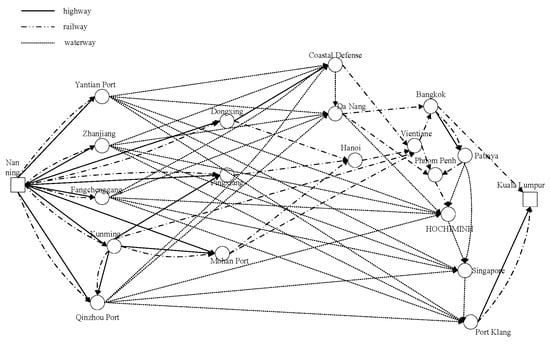
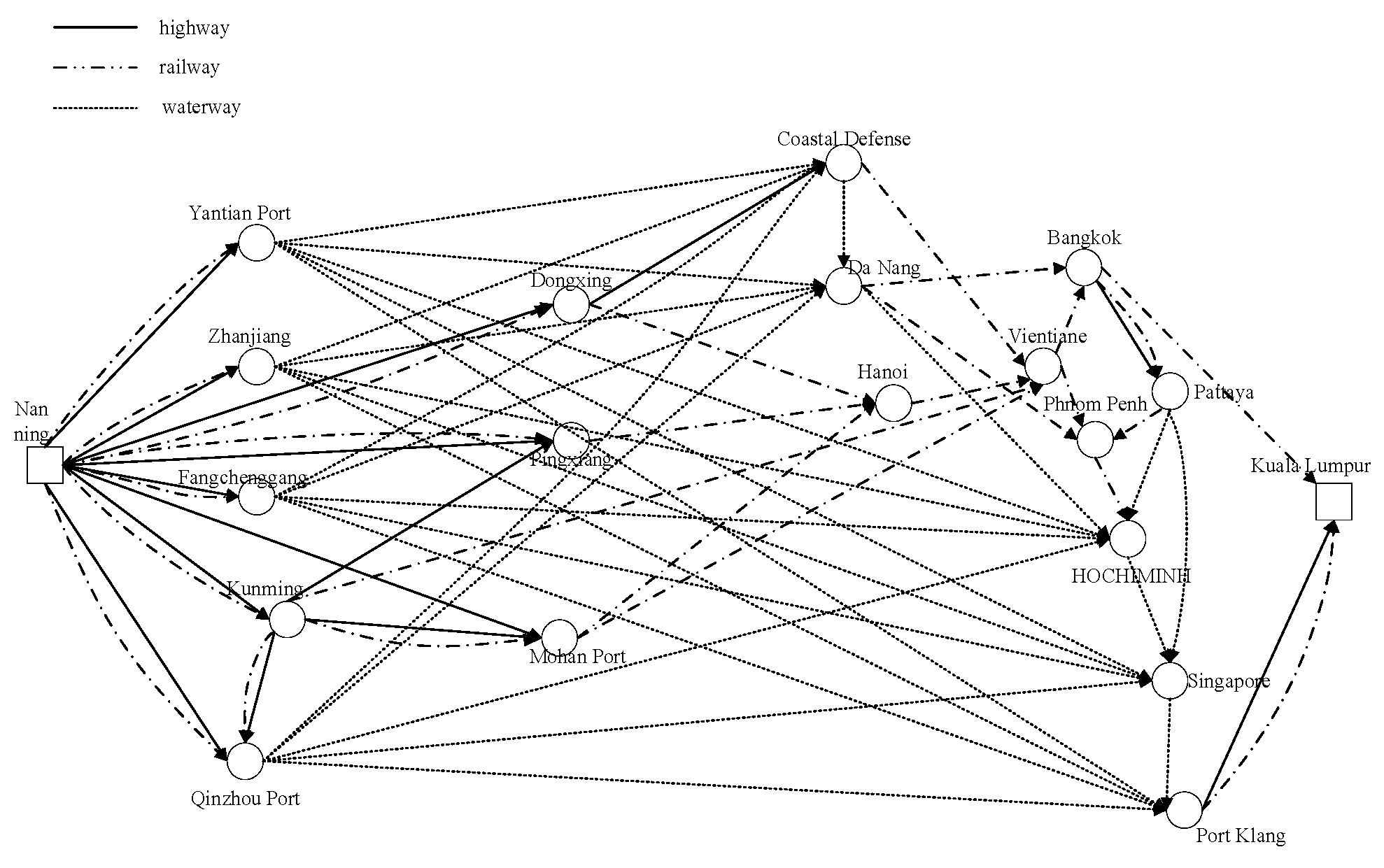
This study takes the Nanning–Kuala Lumpur containerized multimodal transport route as the case study. Since the transshipment nodes along the route are variable, the route optimization requires not only the selection of appropriate transport modes but also the determination of node sequences and transport arcs. Based on transport cost, transit time, and carbon emissions, this section examines the route optimization problem for containerized multimodal transport between Nanning and Kuala Lumpur. Drawing on existing Guangxi–ASEAN transport routes, a containerized multimodal transport network was constructed with Nanning as the origin and Kuala Lumpur as the destination, as shown in Figure 1.

Figure 1. Containerized multimodal transport network from Nanning to Kuala Lumpur.

The Nanning–Kuala Lumpur containerized multimodal transport network consists of 20 node cities. These cities are numbered as shown in Table 2.

Table 2. Coding table of each node city.

No.	City	No.	City	No.	City	No.	City
1	Nanning	6	Kunming	11	Da Nang	16	Phnom Penh
2	Yantian Port	7	Mohan	12	Hanoi	17	Ho Chi Minh City
3	Zhanjiang	8	Ping Xiang	13	Vientiane	18	Singapore Port
4	Fang Chenggang	9	Dong Xing	14	Bangkok	19	Port Klang
5	Qinzhou	10	Haiphong	15	Pattaya	20	Kuala Lumpur

Considering decision preferences related to total transit time, total transport cost, total carbon emissions, and cargo time value cost, the I-NSGA2 algorithm was implemented in Python 3.11 to solve the proposed model and obtained Pareto solution sets for different cargo types. The entropy-weight TOPSIS method was then applied to evaluate the non-dominated solutions and identify a compromise solution, from which the optimal transport plan was determined.

4.2. Data Collection and Processing

To obtain route optimization results that better reflect real operating conditions, the model parameters were set based on empirical data. Key parameters related to transit time, transport cost, and carbon emissions were collected from multiple sources, including published literature, expert interviews, and database retrieval. Inter-node transport distances were measured using Google Maps (v25.40.10.812611599), the Lulu tong App (v5.2.2.20251011), shipping information platforms, and the China Inland Waterway Transport Mileage Table. Freight rates and route information were obtained with reference to the Uniform Transit Tariff Regulations for International Railway Through Freight Transport (2024), the China Railway Atlas, and the China Highway Network Atlas. Carbon emission parameters were determined based on the emission factors reported in the 2006 IPCC Guidelines for National Greenhouse Gas Inventories, supplemented by field investigation and relevant literature.

The transport speeds of different modes are reported in Table 3.

Table 3. Transportation speed parameters for different transportation modes.

Transportation Mode	Transportation Speed/(km/h) Domestic and Overseas Routes
Highway	90
Railway	70
Waterway	28

Based on relevant literature and online data sources, the average values of node operation times are used in the calculation, as shown in Table 4.

Table 4. Node operation time for different transportation modes (h).

Transportation Mode	Highway	Railway	Waterway
Highway	-	0.35	0.4
Railway	0.35	-	0.5
Waterway	0.4	0.5	-

Based on information obtained from freight forwarding companies and online data sources, a unified container freight rate is adopted for domestic road transport. The basic freight rate is set at CNY 9 per container-kilometer, and the fixed container charge is set at CNY 25 per container. With reference to the Uniform Transit Tariff Regulations for International Railway Through Freight Transport and relevant literature, the railway freight calculation rules for transit countries are summarized in Table 5.

Table 5. Transportation costs for different transportation modes.

Transportation	Unit Container Freight Rate (CNY/Container·km)	Fixed Container Fee (CNY/FEU)	Unit Container Freight Rate (USD/TEU·km)
Mode	Domestic		International
Highway	3	25	2
Railway	3.185	440	1.4
Waterway	0.7	-	0.3

For cost conversion, the exchange rate in November 2025 is applied, with USD 1 being equivalent to CNY 7.08.

Since transshipment cost is independent of transport distance, warehousing cost is excluded from the cost calculation. Assuming that handling equipment and operating conditions are broadly comparable across transshipment nodes, the unit transshipment cost for each transport-mode conversion is treated as constant. The corresponding unit transshipment costs between different transport modes are reported in Table 6.

Table 6. Unit container transshipment cost between different transportation modes (CNY/ton).

	Highway	Railway	Waterway
Highway	-	5.5	7.5
Railway	5.5	-	6
Waterway	7.5	6	-

In the process of modeling a cross-border multimodal transport network, a tariff cost is incurred when a transport arc $(i,j)$ crosses a customs boundary, that is, when one endpoint is located within China’s customs territory and the other is located in a foreign customs territory. The tariff rates applied to China’s exports to Southeast Asian countries are reported in Table 7.

Table 7. Tariff rates for China’s exports to Southeast Asian countries.

Entry Country	Myanmar	Thailand	Cambodia	Laos	Vietnam	Malaysia	Singapore
Tariff Rate/%	15	30	15	10	20	0	10

Time-window cost is adopted to describe the time value loss and service penalty caused by the deviations of cargo arrival time at the destination from the expected service time window. Let t denote the arrival time of the transportation task. The hybrid time window is composed of an ideal service time window $\left[e,l\right]$ and an acceptable relaxed time window $\left[E,L\right]$. If condition $t\in \left[e,l\right]$ is satisfied, the arrival time is considered to meet the service requirements, and only the cargo time value cost incurred during transit is included; whereas if condition $t\in [E,e)$ is satisfied, the cargo arrives ahead of schedule, which may incur additional holding and coordination costs such as warehousing and waiting costs as well as loading and unloading coordination costs, thereby generating an early arrival penalty cost; if condition $t\in (l,L]$ is satisfied, the late cargo arrival may lead to a breach of delivery commitments and delays in downstream production, incurring a more severe tardiness penalty cost. Otherwise, the solution is regarded as infeasible. A time value coefficient $\gamma =2$ is introduced into the model to characterize the capital occupation cost of goods per unit time. Meanwhile, fixed early-arrival and late-arrival penalty coefficients, denoted by $\alpha$ and $\beta$, are specified, where ($\beta >\alpha$), to measure the penalty intensity per unit of early or late arrival time. The time-window cost can be expressed as follows: if the arrival time falls within the ideal time window, only the in-transit time cost is calculated according to coefficient $\gamma$; if early or late arrival occurs, penalty terms in the form of $\alpha \gamma (e-t)$ or $\beta \gamma (t-l)$ are superimposed on the basic time value cost, respectively.

Since the carbon emission objective function involves fuel consumption, calorific value and diesel emission factors, relevant data are obtained from related sources and the IPCC Guidelines for National Greenhouse Gas Inventories issued by the Intergovernmental Panel on Climate Change. The carbon emission factors of different transportation modes and the carbon emission coefficients for transshipment between transportation modes within nodes are shown in Table 8 and Table 9, respectively.

Table 8. Carbon emission factor values of different transportation modes.

Transportation Mode	Carbon Emission Factor (g CO2/ton·km)
Highway	62
Railway	22
Waterway	31

Table 9. Reference values of carbon emission coefficients for transfer between different transportation modes.

	Highway	Railway	Waterway
Highway	0	0.12	0.14
Railway	0.12	0	0.11
Waterway	0.14	0.11	0

In addition, carbon emissions are incorporated into the comprehensive cost function by introducing a carbon tax parameter $\theta$, with the carbon tax rate assumed to be USD 20 per ton of CO₂. Based on this setting, the carbon emission cost of a transport route is monetized by multiplying the total emissions by the carbon tax rate, thereby enabling a unified measurement of economic cost and environmental cost.

4.3. Numerical Results and Algorithm Comparison

4.3.1. Numerical Results

The Nanning–Kuala Lumpur containerized multimodal transport network contains 20 node cities. The I-NSGA2 algorithm was configured with a population size of 100, a maximum number of iterations of 100, a crossover probability of 0.9, and a mutation probability of 0.1. The low-value and low time-sensitive cargo scenario assumed a per-container cargo value $V$ of 800, and an annual cargo holding-cost coefficient $\rho$ of 0.1. As a result, 22 non-dominated solutions were obtained for the transport demand of low-value and low time-sensitive cargo, as shown in Table 10.

Table 10. Twenty-two non-dominated solutions for low-value and low-time-sensitive cargo transportation.

	Transportation Scheme	Cost/Yuan	Time/h	Carbon Emissions/t
1	Nanning (Highway)—Fang Chenggang (Waterway)—Port of Singapore (Railway)—Kuala Lumpur	9580.8154	116.6089	14.9087
2	Nanning (Highway)—Fang Chenggang (Waterway)—Port of Singapore (Highway)—Kuala Lumpur	10,431.1658	116.9357	14.6526
3	Nanning (Highway)—Qinzhou (Waterway)—Port of Singapore (Railway)—Kuala Lumpur	10,609.7106	116.1351	17.4238
4	Nanning (Highway)—Qinzhou (Waterway)—Port of Singapore (Highway)—Kuala Lumpur	11,460.0610	116.4619	17.1676
5	Nanning (Highway)—Qinzhou (Waterway)—Port of Ho Chi Minh City (Railway)—Kuala Lumpur	13,613.1817	91.1636	12.1527
6	Nanning (Highway)—Fang Chenggang (Waterway)—Port of Ho Chi Minh City (Railway)—Kuala Lumpur	13,743.1885	90.8368	12.4088
7	Nanning (Railway)—Qinzhou (Waterway)—Port of Ho Chi Minh City (Railway)—Kuala Lumpur	16,008.3318	61.7821	17.5110
8	Nanning (Railway)—Fang Chenggang (Waterway)—Port of Ho Chi Minh City (Railway)—Kuala Lumpur	16,796.3012	91.4779	11.3651
9	Nanning (Highway)—Fang Chenggang (Highway)—Mohan (Railway)—Kuala Lumpur	16,922.4585	91.3511	11.4120
10	Nanning (Railway)—Fang Chenggang (Highway)—Mohan (Railway)—Kuala Lumpur	17,431.2208	91.0432	12.4018
11	Nanning (Highway)—Da Nang (Waterway)—Port of Ho Chi Minh City (Railway)—Kuala Lumpur	17,552.4698	57.2667	38.6285
12	Nanning (Railway)—Da Nang (Waterway)—Port of Ho Chi Minh City (Railway)—Kuala Lumpur	18,917.9095	90.8073	13.9986
13	Nanning (Highway)—Fang Chenggang (Waterway)—Da Nang (Railway)—Port of Ho Chi Minh City (Railway)—Kuala Lumpur	19,243.6235	62.5463	16.5142
14	Nanning (Highway)—Qinzhou (Waterway)—Da Nang (Railway)—Port of Ho Chi Minh City (Railway)—Kuala Lumpur	19,693.6136	80.3379	10.8083
15	Nanning (Railway)—Fang Chenggang (Waterway)—Da Nang (Railway)—Port of Ho Chi Minh City (Railway)—Kuala Lumpur	20,203.3168	68.4414	10.2366
16	Nanning (Railway)—Qinzhou (Waterway)—Da Nang (Railway)—Port of Ho Chi Minh City (Railway)—Kuala Lumpur	20,852.8537	68.7021	9.9713
17	Nanning (Highway)—Dong Xing (Highway)—Vientiane (Railway)—Port of Ho Chi Minh City (Railway)—Kuala Lumpur	21,256.4670	57.2014	8.9200
18	Nanning (Railway)—Dong Xing (Highway)—Vientiane (Railway)—Port of Ho Chi Minh City (Railway)—Kuala Lumpur	26,788.8407	56.3952	18.8709
19	Nanning (Highway)—Ping Xiang (Highway)—Vientiane (Railway)—Port of Ho Chi Minh City (Railway)—Kuala Lumpur	26,796.7815	55.8508	18.3848
20	Nanning (Railway)—Ping Xiang (Highway)—Vientiane (Railway)—Port of Ho Chi Minh City (Railway)—Kuala Lumpur	28,207.5603	56.6514	16.6932
21	Nanning (Highway)—Fang Chenggang (Waterway)—Vientiane (Railway)—Port of Ho Chi Minh City (Railway)—Kuala Lumpur	36,525.5475	55.5624	27.4567
22	Nanning (Railway)—Fang Chenggang (Waterway)—Vientiane (Railway)—Port of Ho Chi Minh City (Railway)—Kuala Lumpur	42,873.2853	55.5792	23.7620

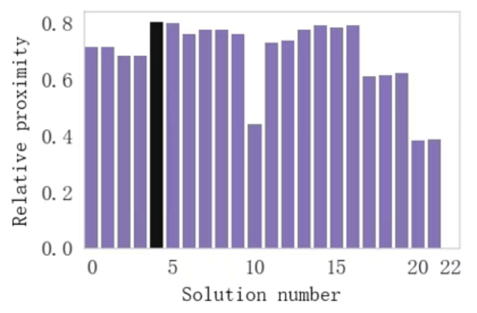
Based on the Pareto solution set obtained above, 22 candidate schemes are generated through multi-objective optimization. For each scheme, the three objective values are represented by $f_{i1},f_{i2},f_{i3}(i=1,\dots ,m)$. The entropy-weight TOPSIS method is then applied to select a preferred solution from these non-dominated solutions.

First, a decision matrix is constructed using the objective values of the Pareto solutions, including total cost, total transit time, and carbon emissions. The three indicators are then normalized to remove dimensional effects and transformed into a consistent preference direction. Next, the information entropy and redundancy of each indicator are calculated using the entropy-weight method, and the objective weight vector w for cost, time, and carbon emissions is obtained. The normalized decision matrix is then multiplied by the corresponding weights to obtain the weighted normalized decision matrix. Subsequently, the positive ideal solution and negative ideal solution are determined, and the Euclidean distances $S_i^{+}$ and $S_i^{-}$ from each scheme to the positive and negative ideal solutions are calculated. The relative closeness coefficient $C_i={\displaystyle \frac{S_i^{-}}{S_i^{+}+S_i^{-}}}$ is then obtained. A larger relative closeness coefficient indicates better overall performance when the three objectives are jointly considered.

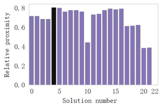
Figure 2 shows the distribution of the relative closeness coefficients of the schemes in the Pareto solution set. According to the entropy-weight TOPSIS results, the recommended compromise transport plan is Nanning–Qinzhou by road, Qinzhou–Ho Chi Minh City Port by waterway transport, and Ho Chi Minh City Port–Kuala Lumpur by rail. The corresponding total cost is CNY 13,613.1817, the total transit time is 91.1636 h, and the total carbon emissions are 12.1527 ton.

Figure 2. Distribution of relative closeness degrees for each scheme in the low-value and low time-sensitivity Pareto solution set.

4.3.2. Comparative Analysis of Algorithms

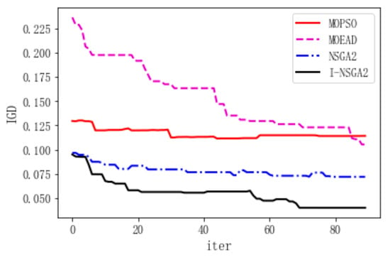
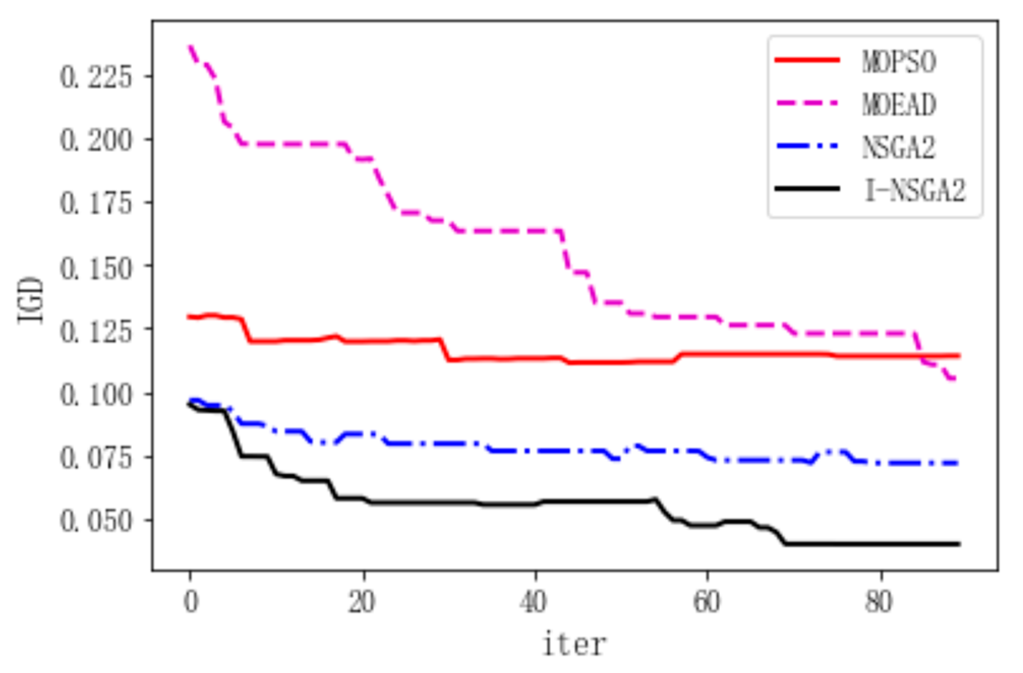
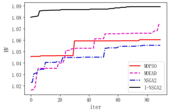
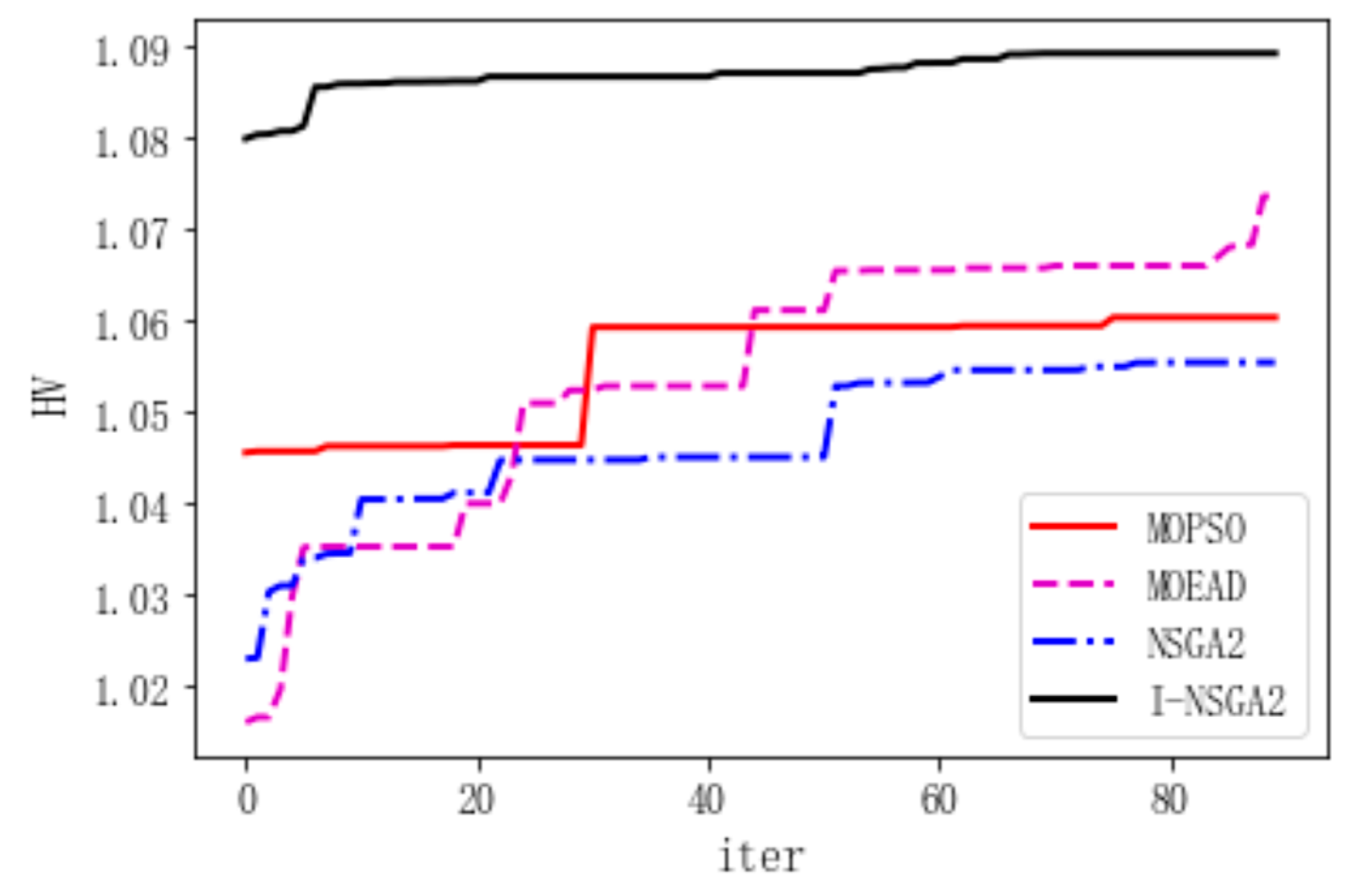
In this study, four algorithms were used to solve the proposed model: multi-objective particle swarm optimization (MOPSO), multi-objective evolutionary algorithm based on decomposition (MOEAD), the standard NSGA-II, and the improved NSGA-II algorithm, denoted as I-NSGA2. The inverted generational distance (IGD) and hypervolume (HV) metrics were employed to quantitatively evaluate the convergence performance and solution-set diversity of each algorithm. Each algorithm was run independently five times. The statistical results are summarized in Table 11, and the variation trends of the two metrics are presented in Figure 3 and Figure 4.

Table 11. Optimal and mean values of each metric for different algorithms.

Algorithm	IGD (Optimal)	HV (Optimal)	IGD (Mean)	HV (Mean)
MOPSO	0.0709	0.9237	0.12976	0.89067
MOEAD	0.0822	0.9142	0.10538	0.90619
NSGA-II	0.0471	0.9149	0.07210	0.88490
I-NSGA2	0.0366	0.9375	0.04022	0.92454

Figure 3. Variation trend of IGD metric for different algorithms.

Figure 4. Variation trend of HV metric for different algorithms.

In multi-objective optimization, a smaller IGD value indicates that the obtained Pareto solution set is closer to the reference Pareto front and therefore has better convergence performance. A larger HV value indicates broader objective-space coverage and better solution-set diversity. I-NSGA2 achieves the lowest IGD and highest HV in terms of both best and mean values. These results suggest that I-NSGA2 can generate a more evenly distributed Pareto solution set with better convergence and diversity, thereby improving the overall performance of the algorithm.

As shown in Figure 3, the IGD values of all four algorithms decrease as the number of iterations increases. I-NSGA2 starts from a relatively low IGD value, decreases rapidly after approximately 20 iterations, and then stabilizes at the lowest final IGD level. This indicates that I-NSGA2 achieves better convergence speed and approximation quality in this numerical example. In comparison, the standard NSGA-II decreases rapidly in the early stage and then stabilizes at an intermediate IGD level, whereas MOPSO converges more slowly and maintains a higher IGD value than NSGA-II. MOEAD remains at the highest IGD level for most iterations, suggesting weaker approximation performance in this case.

Figure 4 shows that the HV values generally increase with the number of iterations. I-NSGA2 rises rapidly in the early stage and stabilizes at the highest final HV value, indicating better objective-space coverage and solution-set diversity. NSGA-II and MOEAD gradually reach similar HV levels in the middle and later stages, although both remain slightly below I-NSGA2. MOPSO exhibits limited HV improvement throughout the iteration process, and its final HV value is lower than those of I-NSGA2 and NSGA-II, indicating relatively weaker coverage of the objective space.

4.4. Sensitivity Analysis

To examine how the proposed model and algorithm respond to variations in key parameters, sensitivity analyses were conducted for the hybrid time-window parameters and the local search perturbation intensity.

For the time-window sensitivity analysis, the allowable time window $[E,L]$ was kept unchanged, while the length of the ideal time window was adjusted to examine the combined effects of time-window settings and penalty costs. The I-NSGA2 algorithm was used to solve the model, with all other parameters held constant. The corresponding transport plans for low-value and low time-sensitive cargo under different ideal time-window lengths are reported in Table 12.

Table 12. Sensitivity analysis on the length of the ideal time window.

Ideal Time Window	Transportation Scheme	Total Cost	Total Time	Carbon Emission
[8,21]	Nanning (Railway)—Fang Chenggang (Waterway)—Port of Singapore (Railway)—Kuala Lumpur	11,302.9426	117.1232	13.9119
[8,20]	Nanning (Highway)—Qinzhou (Waterway)—Port of Ho Chi Minh City (Railway)—Kuala Lumpur	13,613.1817	91.1636	12.1527
[9,21]	Nanning (Railway)—Phnom Penh (Railway)—Port of Ho Chi Minh City (Waterway)—Port of Singapore (Railway)—Kuala Lumpur	17,431.2208	91.0432	12.4018

The population size, maximum number of iterations, and local search perturbation intensity were selected as the key hyperparameters of I-NSGA2. Repeated experiments were conducted under multiple parameter configurations. The IGD and HV metrics, together with their box plots, were used to evaluate the effects of different parameter settings on convergence performance and solution-set diversity, thereby assessing the robustness of the proposed algorithm under parameter variations. The results are reported in Table 13.

Table 13. Sensitivity analysis of varying local search perturbation intensity.

Local Search Perturbation Intensity	Transportation Scheme	IGD		HV
		Optimal	Mean	Optimal	Mean
0.05	Nanning (Highway)—Phnom Penh (Railway)—Port of Ho Chi Minh City (Railway)—Kuala Lumpur	0.03721	0.04419	0.93624	0.92250
0.1	Nanning (Highway)—Qinzhou (Waterway)—Port of Ho Chi Minh City (Railway)—Kuala Lumpur	0.03664	0.04022	0.93745	0.92454
0.2	Nanning (Railway)—Phnom Penh (Railway)—Port of Ho Chi Minh City (Railway)—Kuala Lumpur	0.03880	0.05863	0.92944	0.91961

To examine the stability impact of key parameter fluctuations on optimal route decisions, this paper further conducts a sensitivity analysis on the carbon tax price. With the ideal time window set to [8,20], the local disturbance intensity set to 0.1, and all other parameters held constant, the carbon tax value is set to $10/ton CO₂ and $30/ton CO₂ (with the baseline at $20/ton CO₂). The I-NSGA2 algorithm is employed to solve the Pareto optimal solution sets under each scenario. The analysis investigates the patterns of influence of carbon tax price fluctuations on the route structure, transport mode combination, and total carbon emissions for low-value and time-insensitive cargo, and explores the transmission mechanism of carbon tax policy changes on cross-border container multimodal transport decisions. The results are reported in Table 14.

Table 14. Sensitivity analysis of carbon tax price variations.

Carbon Tax Value ($/ton CO2)	Transportation Scheme	Carbon Emissions (Tons)	IGD	HV
			Optimal	Optimal
10	Nanning (Highway)—Fang Chenggang (Waterway)—Port of Ho Chi Minh City (Railway)—Kuala Lumpur	13.7516	0.03450	0.94020
20	Nanning (Highway)—Qinzhou (Waterway)—Port of Ho Chi Minh City (Railway)—Kuala Lumpur	12.1527	0.03664	0.93745
30	Nanning (Railway)—Fang Chenggang (Waterway)—Singapore Port (Railway)—Kuala Lumpur	10.8700	0.03860	0.93530

Adjusting the ideal time window reshaped the trade-offs among transport cost, transit time, and carbon emissions, thereby influencing the recommended route. Variations in the start and end points of the ideal time window further produced differentiated effects on route selection, indicating that the route optimization results are sensitive to time-window settings in cross-border multimodal transport.

The overall performance of I-NSGA2 under different local search perturbation intensities varied slightly but a clear trend can be observed. A perturbation intensity of 0.10 yielded relatively favorable IGD and HV values among the three tested settings, suggesting that the algorithm achieved a better approximation to the reference Pareto front while maintaining a high degree of solution-set coverage and diversity. When the perturbation intensity was reduced to 0.05 or increased to 0.20, both IGD and HV deteriorated to varying degrees. The substantially larger gap between the mean and best IGD values further indicates reduced convergence stability. These results suggest that insufficient perturbation weakens the algorithm’s ability to escape local optima, whereas overly strong perturbation may disrupt established elite solution structures; both conditions impair stable convergence.

Regarding carbon tax price variation, as the carbon tax increases from $10/ton CO₂ to $30/ton CO₂, the optimal route gradually shifts from road-dominated to rail-dominated. The optimal IGD value increases from 0.03450 to 0.03664 and then to 0.03860, while the optimal HV value decreases from 0.94202 to 0.93745 and then to 0.93530. This indicates that a higher carbon tax intensifies the conflict between cost and carbon emission objectives, thereby increasing the difficulty of solving the multi-objective optimization problem.

5. Conclusions

Taking Guangxi cross-border containerized multimodal transport as the research object, this study develops a multi-objective route optimization model that jointly considers transport cost, transit time, and carbon emissions. An improved NSGA-II algorithm, denoted as I-NSGA2, is proposed and validated through numerical experiments based on the Nanning–Kuala Lumpur containerized multimodal transport network. The main findings are as follows.

(1) The recommended routes obtained by the entropy-weight TOPSIS method show clear differences across cargo types and can provide references for practical decision-making. For low-value and low time-sensitive cargo, the recommended route is Nanning–Qinzhou by highway, Qinzhou–Ho Chi Minh City Port by waterway, and Ho Chi Minh City Port–Kuala Lumpur by railway. This route has the lowest transport cost but the longest transit time, making it more suitable for low-value-added bulk cargo with relatively low delivery-time requirements.

(2) The proposed I-NSGA2 algorithm shows better convergence performance and solution-set diversity than the comparison algorithms. The analysis of the best values, mean values, and convergence curves of IGD and HV shows that I-NSGA2 obtains lower IGD values and higher HV values in most numerical experiments. These results indicate that the Pareto solution set generated by I-NSGA2 is closer to the reference Pareto front and is more evenly distributed.

(3) The sensitivity analysis shows that adjusting the ideal time window drives the optimal route to trade-offs among low cost–long transit time–high emissions and high cost–short transit time–low emissions. Variations in the start and end points of the ideal time window also produce differentiated effects on route selection, indicating that cross-border multimodal transport route optimization is sensitive to time-window settings. In addition, both excessively small and excessively large perturbation intensities lead to marginal decreases in convergence accuracy and solution-set diversity. A perturbation intensity of 0.10 yields relatively stable algorithmic performance and can be used as an initial reference value, which should be further adjusted according to problem scale, network structure, and cargo characteristics. The carbon tax policy exerts a significant regulatory effect on cross-border multimodal transport route selection, meaning that a higher carbon price can effectively guide the shift in transport modes toward lower-carbon options. However, it also imposes higher demands on the algorithm’s optimization capability in multi-objective environments with strong conflicts among objectives.

These findings are consistent with prior evidence that border-related procedural delays, delivery-time flexibility, and carbon-pricing mechanisms can substantially influence freight route choice and modal allocation. Compared with existing studies that examine these factors separately, this study integrates customs-related costs, hybrid time-window penalties, carbon emissions, and carbon tax costs into a unified multi-objective route optimization framework for the Guangxi–ASEAN cross-border container transport corridor. The results therefore provide not only algorithmic evidence on the performance of I-NSGA2, but also practical implications for balancing cost efficiency, delivery reliability, and low-carbon policy requirements in cross-border multimodal transport planning.

References

- Guo, F.; Liang, J.F.; Niu, R.L.; Huang, Z.; Liu, Q. Robust optimization of a procurement and routing strategy for multiperiod multimodal transport in an uncertain environment. Eur. J. Oper. Res. 2025, 327, 115–135. [Google Scholar] [CrossRef] [Scilit]
- Somsai, T.; Pongcharoen, P.; Hicks, C. Optimizing sustainable multimodal distribution networks in the context of carbon pricing, with a case study in the Thai sugar industry. Energy 2024, 298, 131273. [Google Scholar] [CrossRef] [Scilit]
- Han, W.; Chai, H.; Zhang, J.; Li, Y. Research on path optimization for multimodal transportation of hazardous materials under uncertain demand. Arch. Transp. 2023, 67, 91–104. [Google Scholar] [CrossRef] [Scilit]
- Zhou, J.M.; Wei, H.X.; Zhao, Y.Z.; Ma, Y. China-Europe Container Multimodal Transport Path Selection Based on Multi-objective Optimization. Mechatron. Intell. Transp. Syst. 2023, 2, 72–88. [Google Scholar] [CrossRef] [Scilit]
- Chen, M.F.; Liu, Y.Q.; Song, Y.; Sun, Q.; Cong, C.C. Multimodal transport network optimization considering safety stock under real-time information. Discret. Dyn. Nat. Soc. 2019, 2019, 5480135. [Google Scholar] [CrossRef] [Scilit]
- Hamdan, S.; Feillet, D.; Cheaitou, A.; Cariou, P.; Brahimi, N. Optimizing Asia–Europe container network: The Suez Canal and Cape of Good Hope routes in a changing world. Eur. J. Oper. Res. 2025, 325, 167–188. [Google Scholar] [CrossRef] [Scilit]
- Zhang, X.; Jin, F.Y.; Yuan, X.M.; Zhang, H.Y. Low-Carbon Multimodal Transportation Path Optimization under Dual Uncertainty of Demand and Time. Sustainability 2021, 13, 8180. [Google Scholar] [CrossRef] [Scilit]
- Zhou, Y.T.; Li, Z.F.; Duan, W. Exploring the dynamic impact of the Northern Sea Route on China-Europe multimodal transportation competition in the context of the Belt and Road Initiative. Ocean Coast. Manag. 2024, 257, 107346. [Google Scholar] [CrossRef] [Scilit]
- Lv, N. Study on the optimization of the multimodal transport scheme of railway containers. IOP Conf. Ser. Earth Environ. Sci. 2021, 831, 012078. [Google Scholar] [CrossRef] [Scilit]
- Chen, D.X.; Lian, F.; Yang, Z.Z. Assessment of equilibrium accessibility for import/export containers in hub-and-spoke transport network: Impact of international land-sea trade corridor. Transp. Res. Part E Logist. Transp. Rev. 2024, 191, 103747. [Google Scholar] [CrossRef] [Scilit]
- Chen, J.X.; Liao, W.Z.; Yu, C.W. Route optimization for cold chain logistics of front warehouses based on traffic congestion and carbon emission. Comput. Ind. Eng. 2021, 161, 107663. [Google Scholar] [CrossRef] [Scilit]
- Hu, Z.Q.; Wei, Y.G.; Li, Q.; Li, C. Integrated optimization of storage node location and multi-commodities flow routes in multimodal transport networks with carbon emissions consideration. Energy 2025, 328, 136567. [Google Scholar] [CrossRef] [Scilit]
- Ma, J.C.; Wang, X.F.; Yang, K.; Jiang, L. Uncertain programming model for the cross-border multimodal container transport system based on inland ports. Axioms 2023, 12, 132. [Google Scholar] [CrossRef] [Scilit]
- Chen, X.H.; Hu, X.H.; Liu, H.B. Low-carbon route optimization model for multimodal freight transport considering value and time attributes. Socio-Econ. Plan. Sci. 2024, 96, 102108. [Google Scholar] [CrossRef] [Scilit]
- Ge, J.W.; Huang, J.S.; Chao, Y.Y.; Jin, J.; Zhu, S. Optimization of domestic inland transportation routes for imported iron ore with the consideration of carbon costs—A case study of central China. Reg. Stud. Mar. Sci. 2025, 83, 104097. [Google Scholar] [CrossRef] [Scilit]
- Gao, Y.W.; Wang, X.F. Research on optimization model of dynamic distribution path based on intelligent logistics. J. Phys. Conf. Ser. 2020, 1650, 032169. [Google Scholar] [CrossRef] [Scilit]
- Xia, Y.W.; Yang, C.; Chen, B.Q. A path planning method based on improved single player-monte carlo tree search. IEEE Access 2020, 8, 163694–163702. [Google Scholar] [CrossRef] [Scilit]
- Pan, C.H.; Tang, K.S.; Duan, L.M. Intelligent Logistics Information Transmission Demand Objective Optimization Combining Multimodal Transport Dispatch Model. In Proceedings of the 2019 International Conference on Robots & Intelligent System (ICRIS), Haikou, China, 15–16 June 2019; pp. 277–281. [Google Scholar] [CrossRef] [Scilit]
- He, L. Optimization model of shortest distribution path selection in intelligent logistics. J. Phys. Conf. Ser. 2020, 1574, 012171. [Google Scholar] [CrossRef] [Scilit]
- Zhao, Y.B.; Ioannou, P.A.; Dessouky, M.M. Dynamic multimodal freight routing using a co-simulation optimization approach. IEEE Trans. Intell. Transp. Syst. 2019, 20, 2657–2667. [Google Scholar] [CrossRef] [Scilit]
- Bei, H.H.; Yu, M.M.; Yang, T.R.; Murcio, R. Optimization of intermodal transportation routes for perishable goods considering customer satisfaction. Res. Transp. Bus. Manag. 2025, 59, 101261. [Google Scholar] [CrossRef] [Scilit]
- Avetisyan, M.; Heatwole, N.; Rose, A.; Roberts, B. Competitiveness and macroeconomic impacts of reduced wait times at U.S. land freight border crossings. Transp. Res. Part A Policy Pract. 2015, 78, 84–101. [Google Scholar] [CrossRef] [Scilit]
- Caballini, C.; Benzi, M. Fast Corridors: Innovative customs processes and technology to increase supply chain competitiveness. The case of IKEA Italy. Transp. Res. Interdiscip. Perspect. 2023, 21, 100909. [Google Scholar] [CrossRef] [Scilit]
- Madrid, D.; Gurbuz, O.; Vargas, E.; Aldrete, R.M. Border Crossing Delay Cost Analysis: Integration of Various Data Sources in the Direct Cost Estimation Tool. Transp. Res. Rec. J. Transp. Res. Board 2026, online first. [Google Scholar] [CrossRef] [Scilit]
- Jalilifar, E.; Li, X.; Martin, M.; Huang, X. Exploring the potential of market-available connected vehicle data in border crossing time estimation. Trans. Urban Data Sci. Technol. 2024, 3, 31–45. [Google Scholar] [CrossRef] [Scilit]
- Bartlett, A.P.; Qiao, C.; He, Q.; Sadek, A.W. Factors Affecting International Border Crossing Delays Based Upon a Rich Bluetooth Dataset. J. Big Data Anal. Transp. 2020, 2, 33–47. [Google Scholar] [CrossRef] [Scilit]
- Yang, J.; Liang, D.; Zhang, Z.; Wang, H.; Bin, H. Path Optimization of Container Multimodal Transportation Considering Differences in Cargo Time Sensitivity. Transp. Res. Rec. J. Transp. Res. Board 2024, 2678, 1279–1292. [Google Scholar] [CrossRef] [Scilit]
- Ding, L. Multimodal transport information sharing platform with mixed time window constraints based on big data. J. Cloud Comput. 2020, 9, 11. [Google Scholar] [CrossRef] [Scilit]
- Wang, X.; Zhang, P.; Du, Z.; Tian, A.-Q.; Lv, H. Research on Optimization of International Multimodal Transportation Routes Based on Uncertainty Theory. Transp. Res. Rec. J. Transp. Res. Board 2024, 2678, 798–821. [Google Scholar] [CrossRef] [Scilit]
- Xiao, H.; Gong, H.; Wang, X.; Hang, B. Routes Choice in the International Intermodal Networks under the Soft Time Window. Wirel. Commun. Mob. Comput. 2022, 2022, 3355883. [Google Scholar] [CrossRef] [Scilit]
- Demir, E.; Burgholzer, W.; Hrušovský, M.; Arıkan, E.; Jammernegg, W.; Van Woensel, T. A green intermodal service network design problem with travel time uncertainty. Transp. Res. Part B Methodol. 2016, 93, 789–807. [Google Scholar] [CrossRef] [Scilit]
- Qi, Y.; Harrod, S.; Psaraftis, H.N.; Lang, M. Transport service selection and routing with carbon emissions and inventory costs consideration in the context of the Belt and Road Initiative. Transp. Res. Part E Logist. Transp. Rev. 2022, 159, 102630. [Google Scholar] [CrossRef] [Scilit]
- Heinold, A.; Meisel, F. Emission limits and emission allocation schemes in intermodal freight transportation. Transp. Res. Part E Logist. Transp. Rev. 2020, 141, 101963. [Google Scholar] [CrossRef] [Scilit]
- Çapar, İ.; Rump, C.M.; Sawaya, W.; Mohamed, Z.; Alves, J. Green supply chain evolution: A multimodal logistics strategy for capping carbon emissions. Transp. Res. Part E Logist. Transp. Rev. 2025, 202, 104250. [Google Scholar] [CrossRef] [Scilit]
- Yin, C.; Zeng, L.; Fu, X.; Zhong, M. Transition of multimodal transport network under different carbon price scenarios. Transp. Policy 2025, 164, 1–26. [Google Scholar] [CrossRef] [Scilit]
Disclaimer/Publisher’s Note: The statements, opinions and data contained in all publications are solely those of the individual author(s) and contributor(s) and not of MDPI and/or the editor(s). MDPI and/or the editor(s) disclaim responsibility for any injury to people or property resulting from any ideas, methods, instructions or products referred to in the content. |
© 2026 by the authors. Licensee MDPI, Basel, Switzerland. This article is an open access article distributed under the terms and conditions of the Creative Commons Attribution (CC BY) license.