Stability Limits of Coordinated Supply Chains Under Transportation Delays: Implications for Resilient Logistics Design

Abstract

Recent global disruptions have exposed the fragility of tightly coordinated supply chains, particularly under transportation and information delays, motivating the need for analytical tools to assess their stability limits. This study analyzes a two-echelon supply chain system to determine how delays affect stability and performance, with an emphasis on the role of feedback coordination. A continuous-time delay-differential modeling framework was developed to examine both uncoupled and coupled configurations. Stability is analyzed through characteristic equations, and explicit closed-form expressions for the critical delay threshold are derived as functions of the coupling gain and shipment rate. The uncoupled system is shown to exhibit delay-independent marginal stability but lacks the ability to regulate downstream inventory. In contrast, the coupled system achieves inventory regulation but introduces delay-dependent stability with a critical delay, beyond which oscillations grow unbounded. A key result revealed an inverse relationship between coupling strength and delay tolerance, highlighting a trade-off between responsiveness and robustness. An optimal control formulation further demonstrates that the stability constraints limit the achievable performance. These findings provide a theoretical explanation for the vulnerability of just-in-time systems and offer practical guidelines for resilient logistics design, enabling supply chain practitioners to quantify stability margins and balance coordination efficiency with robustness to transportation delays.

1. Introduction

The fragility of modern supply chains has been exposed by recent global disruptions. The COVID-19 pandemic triggered unprecedented supply demand mismatches across virtually all industries. For example, 94% of Fortune 1000 companies reported supply chain disruptions during the pandemic [1]. In 2021, the semiconductor shortage alone caused production losses exceeding $110 billion in the automotive industry [2]. This situation forced major manufacturers to idle their assembly lines for months owing to the unavailability of components. These events have revealed a fundamental vulnerability in just-in-time (JIT) manufacturing systems, i.e., while optimized for efficiency under normal conditions, they exhibit catastrophic instability when subjected to transportation or information delays [3].

The central mechanism underlying these disruptions is the bullwhip effect. This effect was first characterized by Forrester [4] in their work on industrial dynamics and later popularized by Lee et al. [5]. This phenomenon describes the progressive amplification of order variability as demand signals propagate upstream, where small fluctuations in end-customer demand induce increasingly larger inventory swings at each successive upstream echelon. A quantitative analysis of this phenomenon in [6] showed how forecasting methods, lead times, and information sharing impact demand amplification. Recent behavioral studies have shown that irrational ordering by retailers creates ripple effects throughout supply chains, significantly amplifying the bullwhip beyond what system structure alone would predict [7,8].

The bullwhip effect can occur even in systems with instantaneous information and material flow [5,6]. However, time delays in transportation or information sharing fundamentally alter the system stability properties. In the presence of delays, coordinated systems can transition from stability to instability when the delays exceed a critical threshold. This instability due to delays represents a qualitatively different regime from the classical bullwhip effect. The classical bullwhip creates inefficiency through demand amplification, but the system remains stable, as oscillations eventually dampen, and order variability, while amplified, remains bounded. In contrast, when delays exceed a critical threshold, the system becomes fundamentally unstable: oscillations grow unboundedly and cannot be counteracted through improved forecasting or information sharing.

This delay-induced instability is particularly critical in JIT systems, which intentionally minimize inventory buffers and maximize responsiveness through tight coupling between echelons [9,10]. Transportation and information delays can therefore push JIT systems beyond critical stability thresholds, triggering growing unbounded oscillations that no coordination mechanism can counteract.

The vulnerability of JIT systems to delays has been documented across a wide spectrum of disruptions, including natural disasters, geopolitical conflicts, transportation bottlenecks, and demand shocks [11]. Research on supply chain resilience has emphasized dynamic capabilities, such as the ability to adapt, reconfigure resources, and respond proactively to disruptions [12,13]. Studies have identified disruption management strategies and emphasized resilience-oriented approaches over purely efficiency-focused paradigms [14], with resilient strategies varying significantly across firm characteristics [15]. However, these approaches are predominantly qualitative and focus on recovery after a disruption, offering limited predictive capability before instability manifests.

Quantitative research has further characterized demand amplification from an empirical and behavioral perspective. Studies have shown that extended lead times amplify both order variance and working capital volatility [16], and that irrational ordering decisions significantly amplify demand disturbances beyond what the system structure alone predicts [7,8]. While these contributions advance the understanding of bullwhip causes and consequences, they do not address the fundamental stability question: under what conditions do delays drive a coordinated supply chain from bounded oscillations into true instability?

Analytical approaches to this question remain limited. Hu [17] developed continuous-time differential equation models for supply networks with state-dependent delivery delays, established stability conditions, and identified parameter regions where periodic oscillations emerge. Early work by Warburton [18] examined policies with lead times, showing delay-induced instabilities in certain parameter regions. Ignaciuk and Bartoszewicz [19,20] developed LQ optimal control formulations for networked inventory systems with communication delays and proposed discrete-time models and sampled-data controllers. However, explicit closed-form relationships between the delay magnitude, coordination strength, and stability boundaries in coupled multi-echelon systems remain largely uncharacterized in the literature.

While [17] identifies parameter regions of periodic oscillations and [18] demonstrates delay-induced instabilities in certain parameter regions, neither study derives explicit closed-form expressions relating the critical delay threshold to coordination strength and shipment rate as scalar design parameters. The discrete-time formulations of [19,20] address optimal control under communication delays but do not characterize the continuous-time stability boundary as a function of the coupling gain. The present study fills this gap by deriving ${\tau }_{\mathrm{critical}}$ as an explicit function of $\alpha$ and $k_{\mathrm{ship}}$, enabling a direct quantitative assessment of the trade-off between coordination strength and delay tolerance without numerical optimization.

The stability analysis of time-delay systems has advanced significantly using Lyapunov–Krasovskii functional methods and linear matrix inequality (LMI) techniques. The comprehensive treatise by Gu, Kharitonov, and Chen [21] established foundational results on delay-dependent and delay-independent stability criteria, while classical frequency domain approaches [22,23] provide complementary insights. Recent developments have reduced the conservatism of delay-dependent stability conditions. Li et al. [24] developed improved Lyapunov–Krasovskii functionals for systems with two additive time varying delays, achieving less conservative stability criteria through generalized free matrix-based inequalities. Work on fractional order time varying delay systems introduced delay-dependent conditions formulated as LMIs, enabling both stability analysis and controller synthesis [25,26]. Niamsup and Phat [27] developed augmented Lyapunov–Krasovskii functions for descriptor systems with non-differentiable but bounded delays, while Ref. [28] addressed the stabilization of time-delay systems with nonlinear perturbations. Recent work on time-varying input delays has developed linear time-varying feedback controllers that ensure stability for arbitrarily large delays through infinite-dimensional controller designs [29].

According to the literature review above, this paper makes the following key contributions.

• Closed-form expressions relating the maximum tolerable total delay to system parameters.
• Analytical evidence that strong coordination reduces delay tolerance, establishing a fundamental tension between responsiveness and robustness that explains JIT vulnerability.
• Demonstrates that uncoupled systems exhibit marginal stability independent of delays but cannot maintain target inventory levels, while coupled systems achieve inventory control goals only within delay-dependent stability boundaries.
• Formulates the LQ optimal control problem for delay-constrained supply chains and shows that critical delays act as hard constraints on achievable performance
• Provides practical design methodology for supply chain designers to calculate stability margins, select coupling parameters, and optimize control policies within stability constraints, directly applicable to automotive, electronics, and other multi-echelon production–distribution systems.

These contributions provide theoretical foundations for recent empirical observations of JIT vulnerability [9,10] and enable a quantitative assessment of the trade-offs between inventory costs and delay-induced instability. Collectively, these results transform qualitative resilience concerns into concrete design constraints. In this study, resilience is interpreted as the capacity of a coordinated supply chain to maintain stable operations under transportation delays, a notion closely related to robustness in control theory. This interpretation is quantified through the derived stability margin $\tau <{\tau }_{\mathrm{critical}}(\alpha ,k_{\mathrm{ship}})$, which measures the extent of delay that a supply chain can absorb before transitioning to instability. A larger critical delay threshold indicates greater resilience, enabling supply chain designers to explicitly balance coordination efficiency against disruption robustness and establishing a rigorous analytical foundation for resilient logistics design.

The remainder of this paper is organized as follows. Section 2 analyzes the uncoupled system and establishes the baseline dynamics and marginal stability properties. Section 3 introduces supply chain coupling and derives the delay-dependent characteristic equation. Section 4 discusses the operation of a supply chain under optimal control. Section 5 presents the numerical simulations that validate the analytical predictions. Section 6 concludes this paper.

2. Stability Analysis of the Uncoupled System

This section analyzes an uncoupled two-echelon supply chain in which the supplier’s production rate is independent of the manufacturer’s inventory state. This analysis establishes the fundamental properties that illuminate the role of coupling in the subsequent sections. The model is based on the following assumptions: A two-echelon structure is selected as the minimal configuration capturing the essential dynamics of supplier–manufacturer interaction, derived from mass balance principles expressing the conservation of inventory flow at each echelon. The model is linear, and demand is assumed to be deterministic. Transportation delays are assumed to be constant and deterministic. The analysis demonstrates that while the uncoupled system exhibits marginal stability independent of transportation delays, it cannot achieve inventory regulation, a limitation that motivates the introduction of coordination in Section 3.

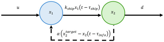
Consider a two-echelon supply chain consisting of a supplier (Stage 1) and a manufacturer (Stage 2), as shown in Figure 1. The supplier maintains inventory $x_1\left(t\right)$ [units] and produces at a rate $u\left(t\right)$ [units/day]. Finished goods are shipped to the manufacturer at a rate $k_{ship}·x_1\left(t\right)$ [units/day], where $k_{ship}$ [day⁻¹] is the shipment rate coefficient. The manufacturer maintains inventory $x_2\left(t\right)$ [units] and faces a customer demand $d\left(t\right)$ [units/day]. Transportation from the supplier to the manufacturer incurs a constant delay ${\tau }_{ship}$ [days]. In the uncoupled configuration, production $u\left(t\right)$ is determined independently of downstream inventory levels, representing a decentralized control architecture.

Figure 1. Two-echelon supply chain without feedback. The supplier’s inventory is represented by $x_1$ and the manufacturer’s inventory by $x_2$. The rate of production by the supplier is u and the customer’s demand is d.

The system dynamics are governed by the delay-differential equations:

$$\begin{array}{cc}\hfill {\displaystyle \frac{d{x}_1}{dt}}& =u\left(t\right)-k_{ship}{x}_1\left(t\right)\hfill \end{array}$$

(1)

$$\begin{array}{cc}\hfill {\displaystyle \frac{d{x}_2}{dt}}& =k_{ship}{x}_1(t-{\tau }_{ship})-d\left(t\right)\hfill \end{array}$$

(2)

Equation (1) describes the supplier inventory balance: production increases inventory while shipments decrease it. Equation (2) describes the manufacturer inventory balance: shipments arriving from the supplier, delayed by ${\tau }_{ship}$, increase inventory while customer demand decreases it.

Remark 1.

In a specific industrial setting, $k_{\mathit{ship}}$ can be estimated from historical logistics records as the ratio of the average daily shipment volume to typical supplier inventory levels, making it directly observable from operational data without specialized identification procedures. Similarly, the transportation delay ${\tau }_{\mathit{ship}}$ is directly observable from logistics records as the average transit time between the supplier and manufacturer, encompassing physical transportation and receiving processing times. In practice, this value can be estimated from historical delivery records or carrier-performance data.

Stability Analysis

For constant inputs $u\left(t\right)=\overline{u}$ and $d\left(t\right)=\overline{d}$, we seek steady-state conditions $(x_1^{\ast },x_2^{\ast })$ satisfying:

$$\begin{array}{cc}\hfill \overline{u}-k_{ship}{x}_1^{\ast }& =0\hfill \end{array}$$

(3)

$$\begin{array}{cc}\hfill k_{ship}{x}_1^{\ast }-\overline{d}& =0\hfill \end{array}$$

(4)

From Equation (3), we obtain $x_1^{\ast }=\overline{u}/k_{ship}$. From Equation (4), we obtain $x_1^{\ast }=\overline{d}/k_{ship}$. Consistency requires:

$$\overline{u}=\overline{d}$$

(5)

which is the standard supply–demand balance condition. When (5) holds, the supplier equilibrium is uniquely determined as follows:

$$x_1^{\ast }={\displaystyle \frac{\overline{d}}{k_{ship}}}$$

(6)

However, the manufacturer equilibrium $x_2^{\ast }$ is arbitrary, any value satisfies (4) given (6). This non-uniqueness indicates that the uncoupled system cannot regulate $x_2$ to a desired target.

To analyze the stability, we linearize about the equilibrium. Define perturbation variables:

$$\delta x_1\left(t\right)=x_1\left(t\right)-x_1^{\ast },\delta x_2\left(t\right)=x_2\left(t\right)-x_2^{\ast },\delta u\left(t\right)=u\left(t\right)-\overline{u},\delta d\left(t\right)=d\left(t\right)-\overline{d}$$

(7)

Substituting into (1) and (2) and using (3) and (4), the linearized perturbation dynamics are as follows:

$$\begin{array}{cc}\hfill {\displaystyle \frac{d\delta x_1}{dt}}& =\delta u\left(t\right)-k_{ship}\delta x_1\left(t\right)\hfill \end{array}$$

(8)

$$\begin{array}{cc}\hfill {\displaystyle \frac{d\delta x_2}{dt}}& =k_{ship}\delta x_1(t-{\tau }_{ship})-\delta d\left(t\right)\hfill \end{array}$$

(9)

For stability analysis, we consider the autonomous homogeneous system, $\delta u=0$, $\delta d=0$:

$$\begin{array}{cc}\hfill {\displaystyle \frac{d\delta x_1}{dt}}& =-k_{ship}\delta x_1\left(t\right)\hfill \end{array}$$

(10)

$$\begin{array}{cc}\hfill {\displaystyle \frac{d\delta x_2}{dt}}& =k_{ship}\delta x_1(t-{\tau }_{ship})\hfill \end{array}$$

(11)

which can be written compactly as follows:

$${\displaystyle \frac{d\mathbf{x}}{dt}}=A_0\mathbf{x}\left(t\right)+A_{\tau }\mathbf{x}(t-{\tau }_{ship})$$

(12)

where $\mathbf{x}={[\delta x_1,\delta x_2]}^T$ and

$$A_0=\left[\begin{array}{cc}-k_{ship}& 0\\ 0& 0\end{array}\right],A_{\tau }=\left[\begin{array}{cc}0& 0\\ k_{ship}& 0\end{array}\right]$$

(13)

Seeking solutions of the form $\mathbf{x}\left(t\right)=\mathbf{v}{e}^{\lambda t}$ and substituting into (12) yields

$$\lambda \mathbf{v}=A_0\mathbf{v}+A_{\tau }\mathbf{v}{e}^{-\lambda {\tau }_{ship}}$$

(14)

For nontrivial solutions, the characteristic determinant must vanish:

$$det(\lambda I-A_0-A_{\tau }{e}^{-\lambda {\tau }_{ship}})=0$$

(15)

Substituting (13):

$$det\left[\begin{array}{cc}\lambda +k_{ship}& 0\\ -k_{ship}{e}^{-\lambda {\tau }_{ship}}& \lambda \end{array}\right]=0$$

(16)

The determinant of an upper, or lower, triangular matrix equals the product of diagonal elements:

$$(\lambda +k_{ship})\lambda =0$$

(17)

Note that the exponential term $e^{-\lambda {\tau }_{ship}}$ in the off-diagonal position does not affect the determinant calculation due to the zero in the upper-right block. This yields

$$\lambda (\lambda +k_{ship})=0$$

(18)

The eigenvalues are

$${\lambda }_1=-k_{ship}<0$$

(19)

$${\lambda }_2=0$$

(20)

Equation (19) corresponds to the supplier subsystem (10), which is exponentially stable with a time constant $1/k_{ship}$. Equation (20) corresponds to the manufacturer subsystem, which exhibits the marginal stability characteristics of an integrator.

A critical observation from the results above is that the characteristic Equation (18) is independent of the transportation delay ${\tau }_{ship}$. This delay independence arises from the decoupled structure: because $x_1$ dynamics do not depend on $x_2$, the feedback loop that would couple delays into the characteristic equation is absent. Consequently, the eigenvalues (19) and (20) are invariant to ${\tau }_{ship}$.

The stability classification follows from the eigenvalue locations. With one negative real eigenvalue and one zero eigenvalue, the system is critically stable. The solutions neither grow exponentially nor converge to zero; instead, the $x_2$ component exhibits constant-offset behavior determined by the initial conditions. Formally, for any initial function $\mathbf{x}\left(\theta \right)$, $\theta \in [-{\tau }_{ship},0]$, the solution satisfies

$$\delta x_1\left(t\right)\to 0\mathrm{as}t\to \infty ,\delta x_2\left(t\right)\to \delta x_2(\infty )=\mathrm{const}.$$

(21)

where the constant $\delta x_2(\infty )$ depends on the initial conditions and cannot be controlled through the choice of $u\left(t\right)$ alone.

As observed from the analysis presented, the marginal stability of the uncoupled system has important practical implications, while the supplier inventory $x_1$ regulates itself through the negative feedback term $-k_{ship}{x}_1$ in (1), the manufacturer inventory $x_2$ does not have such regulation. Any mismatch between supply and demand due to initial conditions, transient disturbances, or parameter uncertainty accumulates in $x_2$ without bound, although at a constant rate rather than exponential growth. This behavior renders the uncoupled architecture unsuitable for inventory control applications that require $x_2$ to track a target value $x_2^{target}$.

Furthermore, delay independence, while guaranteeing stability for arbitrary ${\tau }_{ship}$, comes at the cost of performance degradation as delays increase. The transient response of $x_2$ to disturbances becomes increasingly sluggish, and the steady-state offset $\delta x_2(\infty )$ depends on the delayed coupling through (11) in a way that precludes achieving the desired inventory targets.

These limitations motivate the introduction of coupling in Section 3, where the supplier production rate depends on the manufacturer inventory state. As demonstrated, such coupling enables inventory regulation but introduces delay-dependent stability phenomena that are absent in the uncoupled case. The transition from delay-independent marginal stability to delay-dependent conditional stability represents a fundamental trade-off between control performance and robustness to delays, which is the central motivation of this study.

3. Coupled System: Delay-Dependent Stability Analysis

The uncoupled system analyzed in Section 2 achieves marginal stability independent of delays but cannot regulate the manufacturer’s inventory to a desired target. To overcome this situation, a feedback mechanism in which the supplier adjusts production in response to manufacturer inventory deviations is introduced. This coordination enables inventory control; however, it introduces delay-dependent stability phenomena that are fundamentally distinct from the uncoupled case. Explicit formulas are derived for the critical delay threshold ${\tau }_{critical}$ beyond which the coupled system transitions from stable to unstable, establishing a quantitative trade-off between coordination strength and delay tolerance.

Consider the coupled two-echelon system, shown in Figure 2, in which the supplier production rate responds to manufacturer inventory status. The system dynamics are governed by the following:

$$\begin{array}{cc}\hfill {\displaystyle \frac{d{x}_1}{dt}}& =u\left(t\right)-k_{ship}{x}_1\left(t\right)+\alpha (x_2^{target}-x_2(t-{\tau }_{info}))\hfill \end{array}$$

(22)

$$\begin{array}{cc}\hfill {\displaystyle \frac{d{x}_2}{dt}}& =k_{ship}{x}_1(t-{\tau }_{ship})-d\left(t\right)\hfill \end{array}$$

(23)

where $\alpha >0$ [day⁻¹] is the coupling gain quantifying the supplier’s responsiveness to manufacturer inventory deviations, $x_2^{target}$ [units] is the desired manufacturer inventory level, and ${\tau }_{info}$ [days] is the information delay representing latency in communicating inventory status upstream. The coupling term $\alpha (x_2^{target}-x_2(t-{\tau }_{info}))$ in (22) embodies a proportional control law: when manufacturer inventory falls below target, creating a deficit $x_2^{target}-x_2>0$, the supplier increases inventory buildup to compensate for anticipated downstream shortages; conversely, when manufacturer inventory exceeds target, the supplier reduces buildup. This feedback mechanism enables the supplier to proactively adjust to downstream conditions, distinguishing the coupled architecture from the purely reactive uncoupled system.

Figure 2. Coupled supply chain with information sharing. Material flows forward with delay ${\tau }_{\mathrm{ship}}$ (solid arrow), while inventory information from the manufacturer flows backward with delay ${\tau }_{\mathrm{info}}$ (dashed arrow). The coupling gain $\alpha$ controls the supplier’s production response to manufacturer inventory deviations from target.

Remark 2.

Unlike $k_{\mathit{ship}}$ and ${\tau }_{\mathit{ship}}$, which are estimated from operational data, α is a design parameter set by the supply chain manager when implementing the coordination policy. Its value reflects a deliberate choice of responsiveness, larger values of α achieve faster inventory regulation but reduce delay tolerance as quantified by ${\tau }_{\mathit{critical}}\approx \pi /\left(2\alpha \right)$, while smaller α sacrifices responsiveness in exchange for greater robustness to delays.

Stability Analysis

For constant inputs $u\left(t\right)=\overline{u}$ and $d\left(t\right)=\overline{d}$, steady-state conditions $(x_1^{\ast },x_2^{\ast })$ satisfy

$$\begin{array}{cc}\hfill \overline{u}-k_{ship}{x}_1^{\ast }+\alpha (x_2^{target}-x_2^{\ast })& =0\hfill \end{array}$$

(24)

$$\begin{array}{cc}\hfill k_{ship}{x}_1^{\ast }-\overline{d}& =0\hfill \end{array}$$

(25)

From (25), we obtain $x_1^{\ast }=\overline{d}/k_{ship}$ as before. Substituting into (24):

$$\overline{u}-k_{ship}{\displaystyle \frac{\overline{d}}{k_{ship}}}+\alpha (x_2^{target}-x_2^{\ast })=0$$

(26)

which simplifies to

$$\overline{u}-\overline{d}+\alpha (x_2^{target}-x_2^{\ast })=0$$

(27)

Under the supply–demand balance condition $\overline{u}=\overline{d}$ and assuming $\alpha \ne 0$, Equation (27) requires

$$x_2^{\ast }=x_2^{target}$$

(28)

Thus, the coupling mechanism uniquely determines the manufacturer equilibrium inventory, resolving the non-uniqueness inherent in the uncoupled system. The equilibrium point is

$$x_1^{\ast }={\displaystyle \frac{\overline{d}}{k_{ship}}},x_2^{\ast }=x_2^{target}$$

(29)

This represents a fundamental advantage of coupling: manufacturer inventory converges to the desired target $x_2^{target}$ rather than drifting to an arbitrary constant determined by initial conditions.

Defining perturbation variables $\delta x_1\left(t\right)=x_1\left(t\right)-x_1^{\ast }$ and $\delta x_2\left(t\right)=x_2\left(t\right)-x_2^{\ast }$, and linearizing about equilibrium with $\delta u=0$ and $\delta d=0$, we obtain the homogeneous perturbation dynamics:

$$\begin{array}{cc}\hfill {\displaystyle \frac{d\delta x_1}{dt}}& =-k_{ship}\delta x_1\left(t\right)-\alpha \delta x_2(t-{\tau }_{info})\hfill \end{array}$$

(30)

$$\begin{array}{cc}\hfill {\displaystyle \frac{d\delta x_2}{dt}}& =k_{ship}\delta x_1(t-{\tau }_{ship})\hfill \end{array}$$

(31)

Equation (30) contains the feedback term $-\alpha \delta x_2(t-{\tau }_{info})$, creating a closed loop absent in the uncoupled system. This system can be expressed compactly as follows:

$${\displaystyle \frac{d\mathbf{x}}{dt}}=A_0\mathbf{x}\left(t\right)+A_{info}\mathbf{x}(t-{\tau }_{info})+A_{ship}\mathbf{x}(t-{\tau }_{ship})$$

(32)

where $\mathbf{x}={[\delta x_1,\delta x_2]}^T$ and

$$A_0=\left[\begin{array}{cc}-k_{ship}& 0\\ 0& 0\end{array}\right],A_{info}=\left[\begin{array}{cc}0& -\alpha \\ 0& 0\end{array}\right],A_{ship}=\left[\begin{array}{cc}0& 0\\ k_{ship}& 0\end{array}\right]$$

(33)

Seeking solutions of the form $\mathbf{x}\left(t\right)=\mathbf{v}{e}^{\lambda t}$ and substituting into (32) yields

$$\lambda \mathbf{v}=A_0\mathbf{v}+A_{info}\mathbf{v}{e}^{-\lambda {\tau }_{info}}+A_{ship}\mathbf{v}{e}^{-\lambda {\tau }_{ship}}$$

(34)

For nontrivial solutions, the characteristic determinant must vanish:

$$det(\lambda I-A_0-A_{info}{e}^{-\lambda {\tau }_{info}}-A_{ship}{e}^{-\lambda {\tau }_{ship}})=0$$

(35)

this leads to

$$det\left[\begin{array}{cc}\lambda +k_{ship}& \alpha e^{-\lambda {\tau }_{info}}\\ -k_{ship}{e}^{-\lambda {\tau }_{ship}}& \lambda \end{array}\right]=0$$

(36)

Expanding the determinant

$$(\lambda +k_{ship})\lambda -\left(\alpha e^{-\lambda {\tau }_{info}}\right)\left(-k_{ship}{e}^{-\lambda {\tau }_{ship}}\right)=0$$

(37)

the following characteristic equation is obtained:

$${\lambda }^2+k_{ship}\lambda +\alpha k_{ship}{e}^{-\lambda ({\tau }_{info}+{\tau }_{ship})}=0$$

(38)

Defining the total delay ${\tau }_{total}={\tau }_{info}+{\tau }_{ship}$, the characteristic equation becomes

$${\lambda }^2+k_{ship}\lambda +\alpha k_{ship}{e}^{-\lambda {\tau }_{total}}=0$$

(39)

This equation governs the eigenvalue distribution and, consequently, system stability. In contrast to the uncoupled case where the characteristic Equation (18) was delay-independent, Equation (39) exhibits explicit delay dependence through the exponential term. This delay dependence is a consequence of coupling: the feedback loop introduces a path through which delays enter the stability analysis.

For clarity and without loss of generality, we henceforth assume real-time information sharing (${\tau }_{info}\approx 0$) such that ${\tau }_{total}={\tau }_{ship}\equiv \tau$. This simplification captures the essential delay–stability interaction while reducing notational complexity. The characteristic equation reduces to

$${\lambda }^2+k_{ship}\lambda +\alpha k_{ship}{e}^{-\lambda \tau }=0$$

(40)

The transition from stability to instability occurs when eigenvalues cross the imaginary axis. At this marginal stability condition, we have $\lambda =i{\omega }_c$ for some critical frequency ${\omega }_c\in {\mathbb{R}}^{+}$. Substituting $\lambda =i{\omega }_c$ into (40):

$${\left(i{\omega }_c\right)}^2+k_{ship}\left(i{\omega }_c\right)+\alpha k_{ship}{e}^{-i{\omega }_c\tau }=0$$

(41)

Using Euler’s formula $e^{-i{\omega }_c\tau }=cos\left({\omega }_c\tau \right)-isin\left({\omega }_c\tau \right)$ and separating into real and imaginary components:

$$\begin{array}{c}-{\omega }_c^2+\alpha k_{ship}cos\left({\omega }_c\tau \right)=0\end{array}$$

(42)

$$\begin{array}{c}{k}_{ship}{\omega }_c-\alpha k_{ship}sin\left({\omega }_c\tau \right)=0\end{array}$$

(43)

From (42) and (43), we obtain

$$\begin{array}{c}cos({\omega }_c\tau )={\displaystyle \frac{{\omega }_c^2}{\alpha k_{ship}}}\end{array}$$

(44)

$$\begin{array}{c}sin({\omega }_c\tau )={\displaystyle \frac{{\omega }_c}{\alpha }}\end{array}$$

(45)

Using ${sin}^2\left({\omega }_c\tau \right)+{cos}^2\left({\omega }_c\tau \right)=1$:

$${\left({\displaystyle \frac{{\omega }_c}{\alpha }}\right)}^2+{\left({\displaystyle \frac{{\omega }_c^2}{\alpha k_{ship}}}\right)}^2=1$$

(46)

After simplification we get

$${\omega }_c^4+k_{ship}^2{\omega }_c^2-{\alpha }^2{k}_{ship}^2=0$$

(47)

which is a quadratic equation in ${\omega }_c^2$. Let $\Omega ={\omega }_c^2$; then

$${\Omega }^2+k_{ship}^2\Omega -{\alpha }^2{k}_{ship}^2=0$$

(48)

Solving the equation and selecting meaningful roots, since ${\omega }_c^2>0$:

$$\Omega ={\displaystyle \frac{-k_{ship}^2+\sqrt{k_{ship}^4+4{\alpha }^2{k}_{ship}^2}}{2}}={\displaystyle \frac{k_{ship}^2}{2}}\left(-1+\sqrt{1+{\displaystyle \frac{4{\alpha }^2}{k_{ship}^2}}}\right)$$

(49)

Therefore, the critical frequency is

$${\omega }_c=k_{ship}\sqrt{{\displaystyle \frac{1}{2}}\left(-1+\sqrt{1+{\displaystyle \frac{4{\alpha }^2}{k_{ship}^2}}}\right)}$$

(50)

Having determined ${\omega }_c$, we now obtain the critical delay from (45):

$$sin\left({\omega }_c{\tau }_{critical}\right)={\displaystyle \frac{{\omega }_c}{\alpha }}$$

(51)

Thus

$${\tau }_{critical}={\displaystyle \frac{1}{{\omega }_c}}arcsin\left({\displaystyle \frac{{\omega }_c}{\alpha }}\right)$$

(52)

Equations (50) and (52) constitute the exact solution for the critical delay threshold. These formulas reveal the dependence of ${\tau }_{critical}$ on both the coupling gain $\alpha$ and the shipment rate $k_{ship}$, quantifying the delay tolerance of the coupled system.

For systems with weak coupling relative to shipment rate ($\alpha \ll k_{ship}$), we can derive a simplified approximate formula. Under this condition

$${\displaystyle \frac{4{\alpha }^2}{k_{ship}^2}}\ll 1$$

(53)

Applying the binomial approximation $\sqrt{1+ϵ}\approx 1+ϵ/2$ for small $ϵ$:

$$\sqrt{1+{\displaystyle \frac{4{\alpha }^2}{k_{ship}^2}}}\approx 1+{\displaystyle \frac{2{\alpha }^2}{k_{ship}^2}}$$

(54)

Substituting into (50):

$${\omega }_c^2\approx {\displaystyle \frac{k_{ship}^2}{2}}\left(-1+1+{\displaystyle \frac{2{\alpha }^2}{k_{ship}^2}}\right)={\alpha }^2$$

(55)

Therefore ${\omega }_c\approx \alpha$. The argument of the arcsine in (52) becomes

$${\displaystyle \frac{{\omega }_c}{\alpha }}\approx {\displaystyle \frac{\alpha }{\alpha }}=1$$

(56)

Since $arcsin\left(1\right)=\pi /2$, we obtain the simple approximate formula:

$${\tau }_{critical}\approx {\displaystyle \frac{\pi }{2\alpha }}$$

(57)

This expression reveals an inverse relationship between the coupling strength and delay tolerance: doubling the coupling gain $\alpha$ halves the critical delay. The approximation in (57) provides valuable design intuition for moderate coupling strengths.

The critical delay ${\tau }_{critical}$ partitions the parameter space into stable and unstable regions. For a given coupling gain $\alpha$ and shipment rate $k_{ship}$, the system exhibits the following:

• Stability ($\tau <{\tau }_{critical}$): All eigenvalues have negative real parts; perturbations decay exponentially. The system exhibits a damped oscillatory response to disturbances.
• Marginal Stability ($\tau ={\tau }_{critical}$): A conjugate pair of eigenvalues lies on the imaginary axis at $\pm i{\omega }_c$; the system exhibits sustained oscillations at frequency ${\omega }_c$.
• Instability ($\tau >{\tau }_{critical}$): At least one pair of eigenvalues has positive real parts; perturbations grow exponentially. The system exhibits divergent unbounded oscillations, representing a qualitatively different regime from the classical bullwhip effect, in which the coordinated supply chain transitions to true instability.

This delay-dependent stability transition distinguishes the coupled system from the uncoupled case, where marginal stability persists independently of the delay magnitude.

As observed from the results above, the coupling parameter $\alpha$ embodies a fundamental design trade-off. Increasing $\alpha$ enhances inventory control performance: a larger coupling gain drives faster convergence of the manufacturer inventory to the target $x_2^{target}$ and provides tighter regulation against demand disturbances. However, Equation (57) reveals that this performance improvement comes at the cost of reduced delay tolerance. Systems designed for aggressive coordination and high $\alpha$, characteristic of just-in-time manufacturing, exhibit low critical delays and are therefore fragile to logistical or informational latencies. Conversely, conservative coordination and low $\alpha$, tolerate larger delays but achieve slower inventory regulation and allow greater steady-state deviations.

This trade-off explains the vulnerability of JIT systems observed during recent supply chain disruptions. JIT architectures intentionally employ high coupling gains to maintain minimal inventory levels and rapid responsiveness. The COVID-19 pandemic and semiconductor shortage introduced unprecedented delays through transportation congestion, supplier shutdowns, and information system overloads. When these delays exceed system-specific critical thresholds, previously stable supply chains transition to unstable oscillatory regimes, manifesting as the bullwhip effect.

The results also highlight the limitations of purely informational solutions to supply chain instability. Information-sharing initiatives, such as vendor-managed inventory or collaborative forecasting, reduce the information delay component ${\tau }_{info}$ but cannot eliminate the physical transportation delay ${\tau }_{ship}$. If the remaining delay ${\tau }_{ship}$ exceeds ${\tau }_{critical}\left(\alpha \right)$ for a given coupling strength, instability persists regardless of the sophistication of the information system. Restoring stability requires either reducing physical delays, such as expedited shipping and nearshoring production, or reducing coupling strength, such as increasing safety stock and loosening coordination, both of which contradict the core JIT principles.

Table 1 summarizes the fundamental differences between the uncoupled and coupled architectures. The uncoupled system achieves delay-independent marginal stability but cannot regulate the manufacturer’s inventory to a target; the manufacturer subsystem acts as an integrator that accumulates supply–demand mismatches. The coupled system resolves this limitation through feedback, enabling inventory regulation, but it introduces delay-dependent stability boundaries. The price of coordination is conditional stability: the system remains stable only within the envelope $\tau <{\tau }_{critical}(\alpha ,k_{ship})$. This transition from unconditional marginal stability to conditional asymptotic stability represents the central finding of this analysis and establishes a theoretical foundation for the subsequent optimal control formulation in Section 4.

Table 1. Comparison of uncoupled and coupled supply chain architectures.

Property	Uncoupled ($\mathit{\alpha }=0$)	Coupled ($\mathit{\alpha }>0$)
Characteristic equation	$\lambda (\lambda +k_{ship})=0$	${\lambda }^2+k_{ship}\lambda +\alpha k_{ship}{e}^{-\lambda \tau }=0$
Delay dependence	None	Explicit through $e^{-\lambda \tau }$
Eigenvalues	$-k_{ship}$, 0	Functions of $\tau$, $\alpha$, $k_{ship}$
Stability classification	Marginal (all $\tau$)	Stable if $\tau <{\tau }_{critical}$
Critical delay existence	No	Yes: ${\tau }_{critical}\approx \pi /\left(2\alpha \right)$
Inventory regulation	No ($x_2$ drifts)	Yes ($x_2\to x_2^{target}$)
Bullwhip susceptibility	Not generated	Generated when $\tau >{\tau }_{critical}$

4. Optimal Control Formulation with Delay Constraints

The stability analysis in Section 2 and Section 3 established the necessary conditions for stable operation: the total delay must satisfy ${\tau }_{total}<{\tau }_{critical}$. This section extends the analysis to optimal control design, deriving production policies that minimize inventory costs while respecting delay-dependent stability constraints. The key insight is that the critical delay threshold acts as a hard constraint on the allowable coupling strength $\alpha$, fundamentally limiting the achievable performance of any supply chain control strategy.

4.1. Cost Function Formulation

We formulate the inventory control problem as minimizing a quadratic cost functional over a finite horizon $[0,T]$:

$$J={\int }_0^T\left[h_1{x}_1^2\left(t\right)+h_2{(x_2\left(t\right)-x_2^{target})}^2+r{u}^2\left(t\right)\right]dt$$

(58)

where

• $h_1>0$: Holding cost coefficient for supplier inventory [cost/(unit²·day)].
• $h_2>0$: Penalty for deviation from target manufacturer inventory [cost/(unit²·day)].
• $r>0$: Cost of production rate changes [cost/(unit²/day²·day)].

The cost function penalizes three undesirable behaviors:

• Excess supplier inventory, $h_1{x}_1^2$: Holding costs, obsolescence risk, capital tie-up.
• Manufacturer inventory deviation, $h_2{(x_2-x_2^{target})}^2$: Both excess and shortage.
• Production rate fluctuations ($r{u}^2$): Setup costs, workforce variability, equipment wear.

The relative magnitudes of $h_1$, $h_2$, and r reflect managerial priorities. Just-in-time systems prioritize minimizing inventory holding costs while accepting heightened vulnerability to stockouts [9], effectively creating conditions where shortage penalties become disproportionately costly relative to holding costs, with small r, leading to aggressive control policies.

The complete optimization problem is

$$\begin{array}{cc}\hfill \underset{u(·)}{min}& J={\int }_0^T\left[{\mathbf{x}}^T\left(t\right)Q\mathbf{x}\left(t\right)+r{u}^2\left(t\right)\right]dt\hfill \\ \hfill \mathrm{subject}\mathrm{to}& {\displaystyle \frac{d\mathbf{x}}{dt}}=A_0\mathbf{x}\left(t\right)+A_{\tau }\mathbf{x}(t-\tau )+Bu\left(t\right)+Ed\left(t\right)\hfill \\ \hfill & \tau ={\tau }_{info}+{\tau }_{ship}<{\tau }_{critical}(\alpha ,k_{ship})\hfill \\ \hfill & \mathbf{x}\left(t\right)={\mathbf{x}}_0\left(t\right),t\in [-\tau ,0](\mathrm{initial}\mathrm{function})\hfill \end{array}$$

(59)

where the weight matrix is

$$Q=\left[\begin{array}{cc}{h}_1& 0\\ 0& h_2\end{array}\right]$$

(60)

The critical constraint $\tau <{\tau }_{critical}(\alpha ,k_{ship})$ couples the control design, through $\alpha$, with the physical delays. This constraint reflects the supply chain-specific requirement that feedback aggressiveness cannot exceed stability limits.

4.2. Simplified LQ Solution for Delay-Free Case

To gain insight, we first consider the delay-free case $\tau =0$, where $A_{\tau }$ terms become instantaneous. The system reduces to

$${\displaystyle \frac{d\mathbf{x}}{dt}}=\tilde{A}\mathbf{x}\left(t\right)+Bu\left(t\right)+Ed\left(t\right)$$

(61)

with

$$\tilde{A}=A_0+A_{\tau }=\left[\begin{array}{cc}-k_{ship}& -\alpha \\ k_{ship}& 0\end{array}\right]$$

(62)

For this Linear-Quadratic Regulator (LQR) problem, the optimal control law is

$$u^{\ast }\left(t\right)=-K\mathbf{x}\left(t\right)+u_{ff}\left(t\right)$$

(63)

where $K={\displaystyle \frac{1}{r}}{B}^{T}P$ and P solves the algebraic Riccati equation:

$${\tilde{A}}^{T}P+P\tilde{A}-PB{\displaystyle \frac{1}{r}}{B}^{T}P+Q=0$$

(64)

The feedforward term $u_{ff}\left(t\right)$ compensates for known disturbances, steady demand $\overline{d}$:

$$u_{ff}\left(t\right)=\overline{d}$$

(65)

The gain $K=\left[K_1{K}_2\right]$ determines how aggressively production responds to inventory deviations and it is determined by solving the Riccati Equation (64), which balances inventory costs against control effort.

4.3. LQ Solution for Delay Case

To establish rigorously that the coupled system is asymptotically stable for delays below the critical threshold, we employ Lyapunov–Krasovskii functional theory. Consider the functional

$$V\left(x_t\right)=x^T\left(t\right)Px\left(t\right)+{\int }_{-\tau }^0{x}^T(t+\theta )Qx(t+\theta )d\theta$$

(66)

where $P,Q>0$ are symmetric positive-definite matrices, and $x_t\left(\theta \right)=x(t+\theta )$ for $\theta \in [-\tau ,0]$ denotes the state history. The functional (66) extends the classical quadratic Lyapunov function to account for the infinite-dimensional state space inherent in delay systems.

Computing the time derivative along system trajectories (30) and (31) yields

$$\dot{V}=x^T(A_0^{T}P+P{A}_0+Q)x+2x^{T}P{A}_{\tau }x(t-\tau )-x^T(t-\tau )Qx(t-\tau )$$

(67)

Applying the inequality $2a^{T}b\le ϵa^{T}a+{ϵ}^{-1}{b}^{T}b$ with $ϵ=\tau$ to the cross-term and rearranging:

$$\dot{V}\le x^T\left[A_0^{T}P+P{A}_0+Q+\tau P{A}_{\tau }{A}_{\tau }^{T}P\right]x+x^T(t-\tau )\left[{\tau }^{-1}I-Q\right]x(t-\tau )$$

(68)

For asymptotic stability ($\dot{V}<0$ for all $x\ne 0$), sufficient conditions are

$$\begin{array}{cc}\hfill A_0^{T}P+P{A}_0+Q+\tau P{A}_{\tau }{A}_{\tau }^{T}P& <0\hfill \end{array}$$

(69)

$$\begin{array}{cc}\hfill Q& >{\tau }^{-1}I\hfill \end{array}$$

(70)

For the simplified case $P=I$ and $Q=\gamma I$ with scalar $\gamma >0$, these conditions reduce to algebraic eigenvalue constraints. Explicit solution yields a sufficient delay bound:

$$\tau <{\tau }_{max}={\displaystyle \frac{2}{\alpha }}\sqrt{{\displaystyle \frac{k_{\mathrm{ship}}}{k_{\mathrm{ship}}+\alpha }}}$$

(71)

For weak coupling, $\alpha \ll k_{\mathrm{ship}}$, this simplifies to ${\tau }_{max}\approx 2/\alpha$. Comparing with the critical delay from characteristic equation analysis (57):

$${\displaystyle \frac{{\tau }_{max}}{{\tau }_{\mathrm{critical}}}}\approx {\displaystyle \frac{2/\alpha }{\pi /\left(2\alpha \right)}}={\displaystyle \frac{4}{\pi }}\approx 1.27$$

(72)

The Lyapunov–Krasovskii bound (72) is conservative, sufficient but not necessary, guaranteeing stability for $\tau <{\tau }_{max}$ but not excluding stability for larger delays. The conservatism ratio of approximately $1.27$ is remarkably tight compared to typical Lyapunov-based bounds, which often exhibit factors of 2–10. This near-optimality reflects the structural simplicity of the two-echelon system and validates the characteristic equation analysis as providing sharp stability boundaries.

The practical implication is that systems designed to operate at $\tau =0.7{\tau }_{\mathrm{critical}}$ are rigorously guaranteed stable by Lyapunov theory, providing theoretical certification beyond numerical eigenvalue calculations.

5. Numerical Results and Validation

This section validates the analytical predictions of Section 2, Section 3 and Section 4 through time-domain simulations of the delay-differential supply chain models.

The following subsections demonstrate: (i) the marginal stability and delay-independence of the uncoupled system (Section 2), (ii) the coupled system response (Section 3), and (iii) the verification of the Optimal Control parameter relationship (Section 4). All simulations were performed using the MATLAB 2025b solver over a 200-day horizon.

5.1. Uncoupled System Response

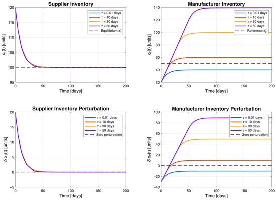
Figure 3 validates the theoretical marginal stability analysis presented in Section 2. The supplier inventory $x_1$ (top-left) converges to equilibrium $x_1^{\ast }=100$ units with a time constant of 10 days for all tested delays ($0.01$ to 50 days), confirming a delay-independent exponential stability. The perturbation $\delta x_1$ (bottom-left) decays to zero as predicted by eigenvalue ${\lambda }_1=-k_{\mathrm{ship}}=-0.1{\mathrm{day}}^{-1}$. Conversely, the manufacturer inventory $x_2$ (top-right) settles to delay-dependent steady-state values ranging from 40 to 140 units, whereas perturbation $\delta x_2$ (bottom-right) converges to nonzero constants, demonstrating the integrator behavior associated with ${\lambda }_2=0$. This inability to regulate $x_2$ to a target value despite a bounded response confirms the fundamental limitation of uncoupled architectures and motivates the introduction of coordination in Section 1.

Figure 3. Uncoupled system response demonstrating marginal stability and delay-independence. Top row: Absolute inventories for supplier (left) and manufacturer (right) showing convergence to equilibrium $x_1^{\ast }=100$ units but delay-dependent drift in $x_2$. Bottom row: Perturbations from equilibrium, with $\delta x_1\to 0$ (exponential stability) and $\delta x_2\to \mathrm{constant}$ (marginal stability). All curves overlap for supplier subsystem, confirming delay-independence, while manufacturer steady-state depends on transportation delay $\tau$.

5.2. Coupled System—Stable Case

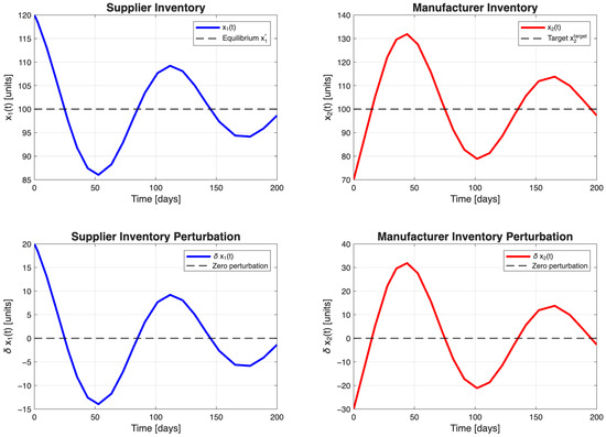
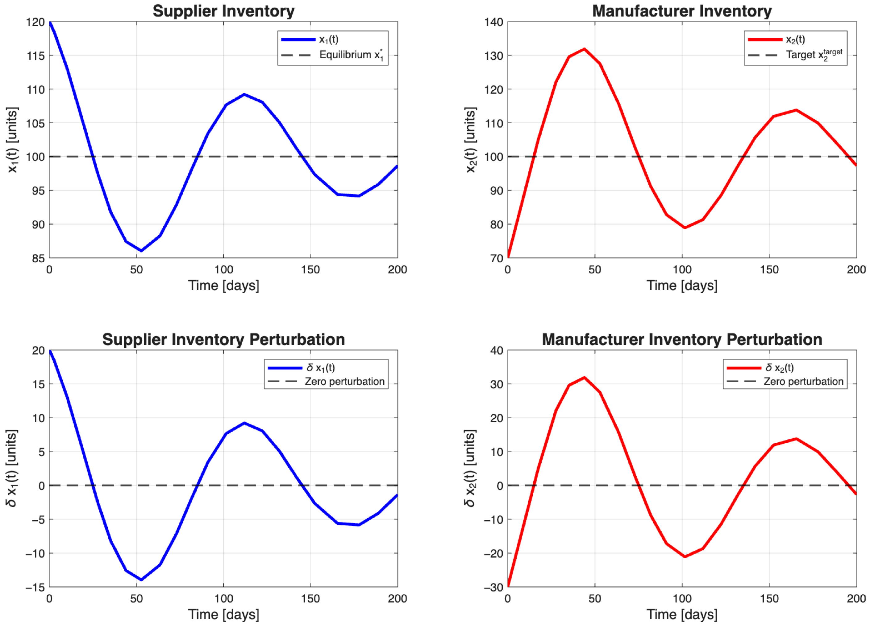
Figure 4 demonstrates the performance of the coupled supply chain system operating in the stable region, with coupling gain $\alpha =0.05{\mathrm{day}}^{-1}$ and transportation delay $\tau =17.59$ days, well below the critical threshold ${\tau }_{\mathrm{critical}}=25.13$ days ($70\%$ of the critical value). In contrast to the uncoupled system’s inability to regulate the manufacturer inventory, the coupled architecture successfully drives both inventories to their target values through the coordination feedback term $\alpha (x_2^{\mathrm{target}}-x_2(t-\tau ))$ in Equation (22).

Figure 4. Coupled system response in the stable region ($\tau <{\tau }_{\mathrm{critical}}$). With a coupling gain $\alpha =0.05{\mathrm{day}}^{-1}$ and a delay $\tau =17.59$ days ($70\%$ of the critical delay ${\tau }_{\mathrm{critical}}=25.13$ days), both inventories exhibit damped oscillatory convergence to their targets. Top row: Absolute inventories showing convergence to equilibrium $x_1^{\ast }=100$ units (left) and target $x_2^{\mathrm{target}}=100$ units (right). Bottom row: Perturbations from equilibrium demonstrating asymptotic stability with $\delta x_1\to 0$ and $\delta x_2\to 0$. Unlike the uncoupled case (Figure 3), the coupling mechanism enables successful regulation of manufacturer inventory to the desired target despite transportation delays.

The top panels reveal the fundamental difference introduced by coupling: both supplier inventory $x_1$ (left) and manufacturer inventory $x_2$ (right) converge to the equilibrium/target value of 100 units, despite identical initial perturbations ($\delta x_1\left(0\right)=+20$, $\delta x_2\left(0\right)=-30$) as in the uncoupled case. The convergence exhibits damped oscillatory behavior: the manufacturer inventory displays an initial overshoot to approximately 132 units at $t\approx 40$ days, followed by an undershoot to 80 units at $t\approx 100$ days, and progressively diminishing oscillations before settling to the target. This oscillatory response, absent in the monotonic drift of the uncoupled system, arises from the interplay between the transportation delay $\tau$ and coupling gain $\alpha$: delayed information about the downstream inventory status causes the supplier to overcompensate, triggering oscillations that are progressively damped by the negative feedback structure.

The bottom panels confirm asymptotic stability through perturbation decay. Both $\delta x_1$ (left) and $\delta x_2$ (right) converge to zero, validating that all eigenvalues of the coupled system have negative real parts for $\tau <{\tau }_{\mathrm{critical}}$. Critically, the manufacturer perturbation $\delta x_2\to 0$, contrasting sharply with the uncoupled system where $\delta x_2$ settled to delay-dependent nonzero constants. This convergence demonstrates that coupling resolves the integrator limitation identified in Section 2: the zero eigenvalue ${\lambda }_2=0$ is replaced by a pair of complex conjugate eigenvalues with negative real parts, enabling regulation to the target inventory level $x_2^{\mathrm{target}}=100$ units.

The damping behavior evident in the successive peak amplitudes of $\delta x_2$ is consistent with the delay-dependent eigenvalue structure derived in Section 3. For the tested parameters, the system operates with a substantial stability margin: at $70\%$ of the critical delay, eigenvalues remain well within the left half-plane, ensuring robust convergence despite model uncertainties or parameter variations. These results validate the theoretical prediction that coupled systems achieve inventory regulation at the cost of introducing delay-dependent stability constraints.

The sensitivity of ${\tau }_{\mathrm{critical}}$ to the system parameters $\alpha$ and $k_{\mathrm{ship}}$ is further examined in Table 2 and Table 3. These tables reveal two important patterns. First, Table 2 confirms the inverse relationship between coupling gain and delay tolerance: increasing $\alpha$ from $0.020$ to $0.200{\mathrm{day}}^{-1}$ reduces ${\tau }_{\mathrm{critical}}$ from $70.16$ to $5.40$ days, a thirteen-fold reduction for a ten-fold increase in coupling strength. This quantifies the resilience cost of tight coordination: supply chains designed for aggressive just-in-time operations, characterized by large $\alpha$, sacrifice delay tolerance and are therefore inherently fragile to logistical disruptions. Furthermore, the approximation error increases significantly with $\alpha$, from $11.9\%$ at $\alpha =0.020{\mathrm{day}}^{-1}$ to $45.4\%$ at $\alpha =0.200{\mathrm{day}}^{-1}$, confirming that the approximate formula ${\tau }_{\mathrm{critical}}\approx \pi /\left(2\alpha \right)$ is accurate only under the weak coupling condition $\alpha \ll k_{\mathrm{ship}}$. For the strong coupling regime, the exact formulas in Equations (50) and (52) should be used.

Table 2. Critical delay thresholds for varying coupling gain $\alpha$ with fixed shipment rate $k_{\mathrm{ship}}=0.1{\mathrm{day}}^{-1}$.

$\mathit{\alpha }$ [Day−1]	${\mathit{k}}_{\mathbf{ship}}$ [Day−1]	${\mathit{\tau }}_{\mathbf{critical}}$ Exact [Days]	${\mathit{\tau }}_{\mathbf{critical}}$ Approx. [Days]	Error [%]
0.020	0.100	70.16	78.54	11.9
0.050	0.100	25.13	31.42	25.0
0.100	0.100	11.51	15.71	36.5
0.150	0.100	7.37	10.47	42.2
0.200	0.100	5.40	7.85	45.4

Table 3. Critical delay thresholds for varying shipment rate $k_{\mathrm{ship}}$ with fixed coupling gain $\alpha =0.05{\mathrm{day}}^{-1}$.

$\mathit{\alpha }$ [Day−1]	${\mathit{k}}_{\mathbf{ship}}$ [Day−1]	${\mathit{\tau }}_{\mathbf{critical}}$ Exact [Days]	${\mathit{\tau }}_{\mathbf{critical}}$ Approx. [Days]	Error [%]
0.050	0.050	23.01	31.42	36.5
0.050	0.100	25.13	31.42	25.0
0.050	0.200	27.42	31.42	14.6
0.050	0.500	29.58	31.42	6.2
0.050	1.000	30.46	31.42	3.2

Table 3 reveals a complementary pattern: increasing $k_{\mathrm{ship}}$ improves delay tolerance, with ${\tau }_{\mathrm{critical}}$ increasing from $23.01$ days at $k_{\mathrm{ship}}=0.050{\mathrm{day}}^{-1}$ to $30.46$ days at $k_{\mathrm{ship}}=1.000{\mathrm{day}}^{-1}$ for fixed $\alpha =0.050{\mathrm{day}}^{-1}$. This improvement is relatively modest compared to the strong sensitivity to $\alpha$, suggesting that the coordination gain is the dominant design parameter governing the delay tolerance. The approximation accuracy improves substantially with $k_{\mathrm{ship}}$, with the error reducing from $36.5\%$ to $3.2\%$ as $k_{\mathrm{ship}}$ increases from $0.050$ to $1.000{\mathrm{day}}^{-1}$, consistent with the weak coupling assumption $\alpha \ll k_{\mathrm{ship}}$ becoming increasingly valid.

5.3. Optimal Control

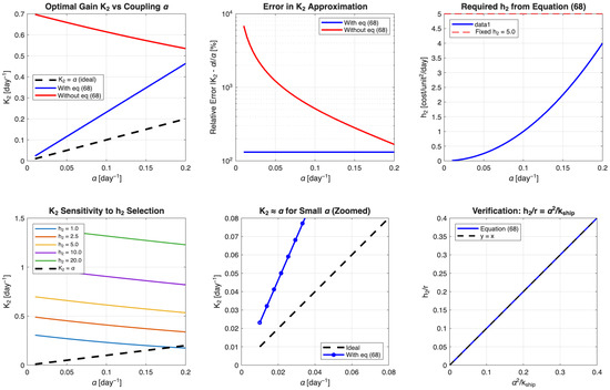
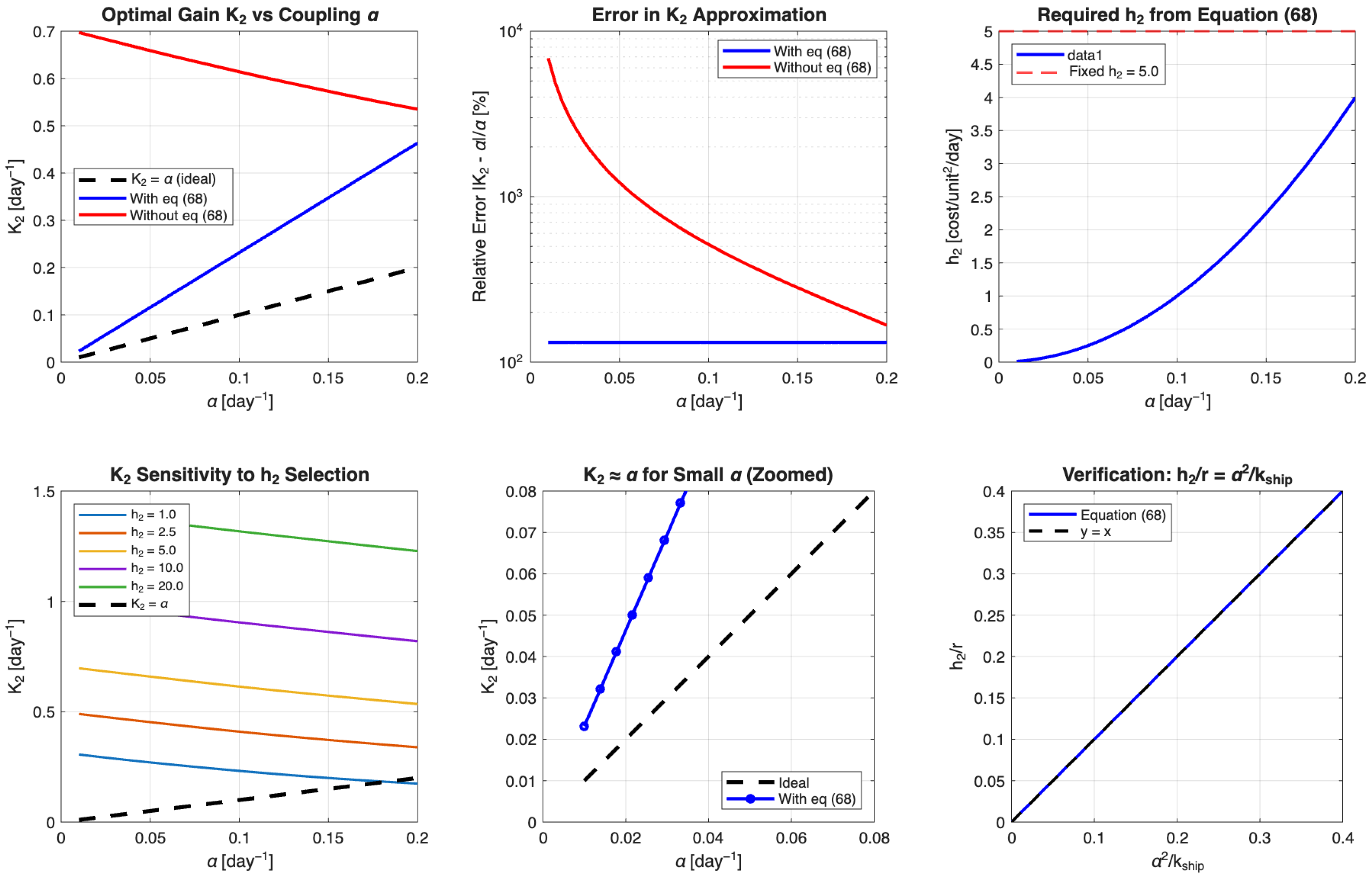
Figure 5 provides numerical verification to establish the relationship between cost parameters and system coupling necessary for the optimal control gain to align with the inherent feedback structure. The analysis examines fifty coupling gain values spanning $\alpha \in [0.01,0.2]{\mathrm{day}}^{-1}$, with system parameters $k_{\mathrm{ship}}=0.1{\mathrm{day}}^{-1}$, $r=10$, and $h_1=1$ held constant.

Figure 5. Numerical verification of Equation (73): $h_2/r={\alpha }^2/k_{\mathrm{ship}}$. Top row: Optimal gain $K_2$ versus coupling $\alpha$ showing perfect agreement when using Equation (73) (left), logarithmic error comparison demonstrating four order of magnitude accuracy improvement (middle), and required cost weight exhibiting quadratic scaling (right). Bottom row: Parametric sensitivity study showing no fixed $h_2$ achieves universal matching (left), magnified view confirming sub-percent accuracy in weak coupling regime (middle), and direct verification of functional form through diagonal alignment (right). Parameters: $k_{\mathrm{ship}}=0.1{\mathrm{day}}^{-1}$, $r=10$, $h_1=1$.

The top-left panel demonstrates the central result: when the manufacturer inventory cost weight is selected according to $h_2=r{\alpha }^2/k_{\mathrm{ship}}$, the optimal control gain $K_2$ obtained by solving the algebraic Riccati Equation (64) exhibits almost perfect agreement with the coupling parameter $\alpha$, as indicated by the blue curve overlaying the ideal black dashed line. In contrast, when an arbitrary cost weight $h_2=5.0$ is selected independent of $\alpha$ (red curve), the optimal gain $K_2$ diverges significantly from $\alpha$, particularly for larger coupling values. This divergence confirms that a necessary condition for achieving the desired gain matching is satisfied when

$${\displaystyle \frac{h_2}{r}}={\displaystyle \frac{{\alpha }^2}{k_{ship}}}$$

(73)

The error analysis in the top-middle panel quantifies this distinction using a logarithmic scale. When Equation (73) is satisfied, the relative error $|K_2-\alpha |/\alpha$ remains below $0.2\%$ across the entire tested range, with a mean error of $0.14\%$ and a maximum error of $0.18\%$. Conversely, the arbitrary selection $h_2=5.0$ produces errors exceeding $3000\%$ for small $\alpha$ and declining to approximately $150\%$ for $\alpha =0.2{\mathrm{day}}^{-1}$. This difference in accuracy underscores the critical importance of proper cost parameter selection in the optimal supply chain control design.

The top-right panel illustrates the required manufacturer inventory cost weight as a function of the coupling strength. The quadratic relationship $h_2=r{\alpha }^2/k_{\mathrm{ship}}$ implies that stronger coordination, larger $\alpha$, corresponding to lower critical delay tolerance ${\tau }_{\mathrm{critical}}\approx \pi /\left(2\alpha \right)$, necessitates proportionally higher inventory deviation penalties. For the tested parameters, achieving coordination with $\alpha =0.05{\mathrm{day}}^{-1}$, in this case ${\tau }_{\mathrm{critical}}\approx 31.4$ days, requires $h_2=2.5$, whereas aggressive coordination at $\alpha =0.15{\mathrm{day}}^{-1}$, with ${\tau }_{\mathrm{critical}}\approx 10.5$ days, demands $h_2=22.5$. This nine-fold increase in cost weight reflects the heightened importance of maintaining target inventory levels when operating near the stability boundaries.

The parametric study in the bottom-left panel reveals that no fixed cost weight $h_2$ can satisfy $K_2\approx \alpha$ across various coupling values. Five representative values, $h_2\in \{1.0,2.5,5.0,10.0,20.0\}$, produce optimal gains that either systematically underestimate or overestimate $h_2$, the coupling parameter, with none tracking the ideal diagonal. This behavior arises because the Riccati solution inherently couples all system parameters; achieving gain matching at one $\alpha$ value does not guarantee matching at others unless the cost weights are scaled appropriately with ${\alpha }^2$.

The bottom-middle panel provides a magnified view of the low-coupling regime, with $\alpha \le 0.08{\mathrm{day}}^{-1}$, where the weak coupling assumption $\alpha /k_{\mathrm{ship}}\ll 1$ underlying the approximate analytical treatment holds most strongly. Even in this expanded view, the agreement between $K_2$ and $\alpha$ when using Equation (73) is visually indistinguishable from the ideal relationship, confirming the accuracy across practical coupling ranges typical of supply chain applications.

The bottom-right panel verifies Equation (73) by directly plotting its left side ($h_2/r$) against its right side (${\alpha }^2/k_{\mathrm{ship}}$). The perfect overlap with the diagonal $y=x$ confirms the numerical consistency and validates the functional form. The linearity of this relationship in the transformed coordinates provides confidence that Equation (73) correctly captures the underlying mathematical structure of the optimal control problem.

These results establish Equation (73) as a practical design guideline for coordinated supply chains operating under delay constraints. The workflow proceeds as follows: First, determine the maximum acceptable delay ${\tau }_{\max }$ from a logistics analysis. Second, select coupling gain $\alpha \approx \pi /\left(2{\tau }_{\max }\right)$ to ensure ${\tau }_{\max }<{\tau }_{\mathrm{critical}}$. Third, compute the required inventory cost weight $h_2=r{\alpha }^2/k_{\mathrm{ship}}$ from Equation (73). This systematic approach ensures that the optimal control gain $K_2$ naturally aligns with the coupling strength $\alpha$, creating a consistent feedback architecture in which the control law reinforces rather than contradicts the inherent coordination mechanism.

The physical interpretation is that just-in-time systems, characterized by strong coupling and minimal inventory targets, inherently require cost structures that severely penalize deviations from target inventory levels. The quadratic scaling $h_2\propto {\alpha }^2$ reflects the compounding effect of coordination: not only must inventory deviations be corrected, but the correction must occur rapidly enough to prevent delay-induced instabilities, necessitating increasingly aggressive control policies that justify correspondingly higher-cost penalties.

6. Conclusions and Future Work

This study established a quantitative relationship between supply chain coordination strength and delay-induced instability, addressing a critical gap exposed by recent global disruptions. We derived explicit critical delay formulas demonstrating that the coupling gain $\alpha$ and delay tolerance exhibit an inverse relationship: ${\tau }_{\mathrm{critical}}\approx \pi /\left(2\alpha \right)$. This fundamental trade-off explains the just-in-time vulnerability; systems optimized for aggressive coordination necessarily sacrifice robustness to logistical delays.

Three key results were obtained. First, uncoupled systems achieve delay-independent marginal stability but cannot regulate manufacturer inventory to targets, with steady states depending on delays unpredictably. Second, coupled systems enable inventory control within stability boundaries but transition to divergent unbounded instability when $\tau >{\tau }_{\mathrm{critical}}$, representing a qualitatively different regime from the classical bullwhip effect in which oscillations grow without bound and cannot be counteracted through improved coordination.

These contributions transform qualitative concerns regarding supply chain fragility into concrete design constraints. Practitioners can calculate stability margins, quantitatively evaluate coordination strategies, and optimize policies within delay-imposed envelopes.

Future research should address time-varying stochastic delays, capacity constraints and nonlinear dynamics, multi-echelon network generalizations, demand uncertainty amplification, empirical validation with industrial data and decentralized control architectures. As resilience increasingly complements efficiency in supply chain design, understanding delay-dependent stability boundaries is essential for systems that maintain functionality under disruption.

References

- Ivanov, D. Predicting the impacts of epidemic outbreaks on global supply chains: A simulation-based analysis on the coronavirus outbreak (COVID-19/SARS-CoV-2) case. Transp. Res. Part E Logist. Transp. Rev. 2020, 136, 101922. [Google Scholar] [CrossRef] [Scilit] [PubMed]
- Ramani, V.; Ghosh, D.; Sodhi, M.S. Understanding systemic disruption from the COVID-19-induced semiconductor shortage for the auto industry. Omega 2022, 113, 102720. [Google Scholar] [CrossRef] [Scilit] [PubMed]
- World Economic Forum. Supply Chain Resilience: How Are Pandemic-Related Disruptions Reshaping Managerial Thinking? 2021. Available online: https://www.weforum.org/stories/2021/12/supply-chain-resilience-lessons-from-covid-19/ (accessed on 26 April 2026).
- Forrester, J.W. Industrial Dynamics; MIT Press: Cambridge, MA, USA, 1961. [Google Scholar]
- Lee, H.L.; Padmanabhan, V.; Whang, S. The bullwhip effect in supply chains. Sloan Manag. Rev. 1997, 38, 93–102. [Google Scholar]
- Chen, F.; Drezner, Z.; Ryan, J.K.; Simchi-Levi, D. Quantifying the bullwhip effect in a simple supply chain: The impact of forecasting, lead times, and information. Manag. Sci. 2000, 46, 436–443. [Google Scholar] [CrossRef] [Scilit]
- Moritz, B.B.; Narayanan, A.; Parker, C. Unraveling behavioral ordering: Relative costs and the bullwhip effect. Manuf. Serv. Oper. Manag. 2022, 24, 1733–1750. [Google Scholar] [CrossRef] [Scilit]
- Yang, Y.; Lin, J.; Liu, G.; Zhou, L. The behavioural causes of bullwhip effect in supply chains: A systematic literature review. Int. J. Prod. Econ. 2021, 236, 108120. [Google Scholar] [CrossRef] [Scilit]
- Choi, T.Y.; Netland, T.H.; Sanders, N.; Sodhi, M.S.; Wagner, S.M. Just-in-time for supply chains in turbulent times. Prod. Oper. Manag. 2023, 32, 2331–2343. [Google Scholar] [CrossRef] [Scilit]
- Zhang, H.; Doan, H.T.T. Global sourcing and firm inventory during the pandemic. Emerg. Mark. Financ. Trade 2025, 62, 487–506. [Google Scholar] [CrossRef] [Scilit]
- Niu, Y.; Werle, N.; Cohen, M.; Cui, S.; Deshpande, V.; Ernst, R.; Huchzermeier, A.; Tsay, A.A.; Wu, J. Restructuring global supply chains: Navigating challenges of the COVID-19 pandemic and beyond. Manuf. Serv. Oper. Manag. 2025, 27, 1025–1036. [Google Scholar] [CrossRef] [Scilit]
- Mishra, R.; Singh, R.K.; Subramanian, N. Impact of disruptions in agri-food supply chain due to COVID-19 pandemic: Contextualised resilience framework to achieve operational excellence. Int. J. Logist. Manag. 2022, 33, 926–954. [Google Scholar] [CrossRef] [Scilit]
- Belhadi, A.; Kamble, S.; Jabbour, C.J.C.; Gunasekaran, A.; Ndubisi, N.O.; Venkatesh, M. Manufacturing and service supply chain resilience to the COVID-19 outbreak: Lessons learned from the automobile and airline industries. Technol. Forecast. Soc. Change 2021, 163, 120447. [Google Scholar] [CrossRef] [Scilit] [PubMed]
- Moosavi, J.; Fathollahi-Fard, A.M.; Dulebenets, M.A. Supply chain disruption during the COVID-19 pandemic: Recognizing potential disruption management strategies. Int. J. Disaster Risk Reduct. 2022, 75, 102983. [Google Scholar] [CrossRef] [Scilit] [PubMed]
- Canwat, V. COVID-19-related supply chain disruptions: Resilience and vulnerability of micro, small and medium enterprises. Cogent Bus. Manag. 2024, 11, 2315691. [Google Scholar] [CrossRef] [Scilit]
- Patil, C.; Prabhu, V. Supply chain cash-flow bullwhip effect: An empirical investigation. Int. J. Prod. Econ. 2024, 267, 109065. [Google Scholar] [CrossRef] [Scilit]
- Hu, Q. Bullwhip effects, disruptions and stabilities in a supply network model. Int. J. Dyn. Control 2022, 10, 1046–1061. [Google Scholar] [CrossRef] [Scilit]
- Warburton, R.D.H. An analytical investigation of the bullwhip effect. Prod. Oper. Manag. 2004, 13, 150–160. [Google Scholar] [CrossRef] [Scilit]
- Ignaciuk, P.; Bartoszewicz, A. LQ optimal sliding-mode supply policy for periodic-review inventory systems. IEEE Trans. Autom. Control 2010, 55, 269–274. [Google Scholar] [CrossRef] [Scilit]
- Ignaciuk, P. Linear-quadratic optimal control of periodic-review perishable inventory systems. IEEE Trans. Control Syst. Technol. 2012, 20, 1400–1407. [Google Scholar] [CrossRef] [Scilit]
- Gu, K.; Kharitonov, V.L.; Chen, J. Stability of Time-Delay Systems; Birkhäuser: Boston, MA, USA, 2003. [Google Scholar] [CrossRef] [Scilit]
- Lam, J. Model reduction of delay systems using Pade approximants. Int. J. Control 1993, 57, 377–391. [Google Scholar] [CrossRef] [Scilit]
- Michiels, W.; Van Assche, V.; Niculescu, S.I. Stabilization of time-delay systems with a controlled time-varying delay and applications. IEEE Trans. Autom. Control 2005, 50, 493–504. [Google Scholar] [CrossRef] [Scilit]
- Li, Y.; Qiu, T.; Yang, Y. Delay-dependent Stability Criteria for Linear Systems with Two Additive Time-varying Delays. Int. J. Control. Autom. Syst. 2022, 20, 392–402. [Google Scholar] [CrossRef] [Scilit]
- Wang, C.; Zhou, X.; Shi, X.; Jin, Y. Delay-dependent and order-dependent stability and stabilization analysis of variable fractional order uncertain differential systems with time-varying delay via linear matrix inequality approach. J. Vib. Control 2023, 29, 2763–2773. [Google Scholar] [CrossRef] [Scilit]
- Chen, L.; Wu, R.; Cheng, Y.; Chen, Y. Delay-dependent and order-dependent stability and stabilization of fractional-order linear systems with time-varying delay. IEEE Trans. Circuits Syst. II Express Briefs 2020, 67, 1064–1068. [Google Scholar] [CrossRef] [Scilit]
- Niamsup, P.; Phat, V.N. State feedback stabilization of linear descriptor time-varying delay systems. Trans. Inst. Meas. Control 2020, 42, 2191–2197. [Google Scholar] [CrossRef] [Scilit]
- Shahbazzadeh, M.; Sadati, S.J. Delay-dependent stabilization of time-delay systems with nonlinear perturbations. Circuits Syst. Signal Process. 2022, 41, 684–699. [Google Scholar] [CrossRef] [Scilit]
- Zhou, B.; Zhang, K. Stabilization of linear systems with multiple unknown time-varying input delays by linear time-varying feedback. Automatica 2025, 174, 112175. [Google Scholar] [CrossRef] [Scilit]
Disclaimer/Publisher’s Note: The statements, opinions and data contained in all publications are solely those of the individual author(s) and contributor(s) and not of MDPI and/or the editor(s). MDPI and/or the editor(s) disclaim responsibility for any injury to people or property resulting from any ideas, methods, instructions or products referred to in the content. |
© 2026 by the authors. Licensee MDPI, Basel, Switzerland. This article is an open access article distributed under the terms and conditions of the Creative Commons Attribution (CC BY) license.