


Abstract
Studies explaining the variation in educational outcomes across countries, when based on “black box” models that provide high accuracy but struggle to present the decision-making mechanism transparently, carry the risk of producing limited interpretations for policy discussions. This study examines the system-level relational patterns through which the subcomponents of the Heritage Foundation Index of Economic Freedom distinguish country-average low–medium–high PISA performance profiles in mathematics, reading, and science, and interprets these patterns using machine learning and explainable artificial intelligence (XAI). The analysis draws on approximately twenty years of nominal country-year records covering 76 countries. The study design proceeds through a classification approach, treating country performance as low–medium–high profiles; thus, model outputs are presented on an interpretable reference plane for cross-country comparisons. The findings indicate that the models demonstrate consistent generalization ability in distinguishing performance profiles and that the XAI layer produces explanations that make the model’s reasoning visible in a verifiable manner. The explanation results indicate that components representing institutional trust (such as government integrity and property rights) produce strong, recurring signals alongside higher performance profiles in all three areas; while components such as public expenditure and tax burden can emerge as balancing/suppressing signals in some scenarios. Rather than offering causal policy implications, these findings transparently reveal the structural areas that stand out in distinguishing performance profiles in cross-country comparisons, thus providing an explainable, replicable evidence base for comparative analysis and further research.
1. Introduction
Large-scale international student assessments provide a critical reference framework for countries to monitor their education systems comparatively and support comparative evaluation of structural priorities. The OECD’s Programme for International Student Assessment (PISA) not only makes learning outcomes at the student level visible but also strengthens discussions about the structural conditions that give rise to cross-country differences. Therefore, the literature interpreting PISA results examines numerous variable groups, such as socioeconomic structure, institutional characteristics, and macro-level indicators, to explain the signals of educational achievement. However, attempts to explain educational performance at the country-level face two fundamental challenges. First, multidimensional results such as PISA may contain non-linear relationships and interactions when evaluated alongside economic, institutional, and governance factors. While classical statistical models may provide a robust framework in some cases, their capacity to capture complex patterns may be limited. Second, modern machine learning approaches that provide stronger predictions often face the “black box” criticism: even if models can produce high accuracy, their transferability to comparative interpretation and evidence-informed discussion may be weakened when the patterns underlying the decision are not presented in a sufficiently transparent manner.
A growing body of literature has examined the signals of cross-country variation in educational outcomes from multiple analytical perspectives. First, within the field of institutional economics, several studies emphasize the role of economic institutions and governance quality in shaping human capital formation [1,2]. In this line of research, dimensions such as property rights, regulatory quality, and government integrity are associated with more efficient allocation of resources and improved public service delivery, including education. These studies indicate that institutional structures may indirectly influence educational outcomes through systemic channels rather than direct policy interventions [3,4].
Second, extensive empirical literature focuses on cross-country PISA performance differences, highlighting the importance of both structural and contextual factors. This body of work examines variables such as socioeconomic composition, educational expenditure, school autonomy, and cultural factors, often using regression-based or multilevel modeling approaches [5]. While these studies provide valuable insights into average effects and within-country variation, they typically rely on parametric assumptions and may face limitations in capturing complex, non-linear interactions across multiple dimensions.
Third, recent advances in data science have introduced machine learning and explainable artificial intelligence (XAI) into the analysis of social and educational outcomes. Machine learning models offer strong predictive capabilities and the ability to model high-dimensional relationships without restrictive functional form assumptions. However, conventional “black-box” approaches often lack transparency, limiting their usefulness for policy-oriented interpretation. The emergence of XAI techniques addresses this limitation by making model decision processes interpretable and traceable, thereby enhancing analytical accountability.
Despite these advances, a clear gap remains in the literature. Existing studies either emphasize theoretical or econometric explanations with limited dimensional flexibility, or adopt high-performance predictive models with limited interpretability. Moreover, there is a lack of approaches that conceptualize educational outcomes in terms of performance profiles (e.g., low–medium–high) and examine how institutional structures relate to these profiles in a transparent and comparable manner across countries. Accordingly, this study addresses this gap by proposing a classification-based, explainable machine learning framework that links economic freedom components to cross-country PISA performance profiles, providing an interpretable and multi-dimensional perspective on structural differences.
Against this background, explainable artificial intelligence (XAI) offers a useful framework for addressing the dual need for predictive capacity and interpretability in educational analytics. The fundamental promise of XAI is to make the decision logic visible in a verifiable manner while maintaining model performance, thereby bridging the gap between “prediction” and “interpretation.” The use of XAI in studies aimed at classifying or predicting PISA performance at the country-level can contribute to the evaluation of results not merely as statistical findings but as a basis for discussion. However, for this contribution to be meaningful, it is not only important to produce explanations, but also to establish the interpretation line of the study cautiously through relational patterns, without making claims of causality. This study focuses on the components of the Index of Economic Freedom (IEF), a set of indicators related to economic institutions and governance, while discussing the structural factors that shape educational achievement at the country-level. Since the IEF subcomponents bring together different dimensions related to institutional trust and market functioning, they provide a functional framework for examining which signals emerge more systematically in distinguishing performance profiles between countries. In this context, the study treats the country’s average performances in PISA’s mathematics (PISAM), reading (PISAR), and science (PISAS) domains as performance profiles to facilitate interpretation and examines which IEF components these profiles appear alongside.
Accordingly, the central research question of this study is: Which relational patterns do the subcomponents of the Heritage Foundation Index of Economic Freedom exhibit in distinguishing country-average low–medium–high PISA performance profiles in mathematics, reading, and science, and how can these patterns be interpreted through an explainable artificial intelligence framework? By formulating the problem in this way, the study focuses on system-level profile differentiation.
The study’s methodological approach is two-layered. In the first layer, the separability of countries’ performance profiles is tested using modern machine learning models; in the second layer, explanations are generated using a fiXAIt-based XAI framework to make the patterns behind the separation transparent. This approach allows for a comparative discussion of signals that may vary by domain, rather than producing a singular list of “only the most important variables.” Thus, the findings can be reported in a way that helps identify which structural domains may warrant closer analytical attention in cross-country comparisons. This study aims to make three key contributions to the literature. First, it goes beyond analyses that merely describe PISA performance at the country-level by demonstrating the separability of performance profiles using modern machine learning. Second, thanks to the XAI layer, the patterns generating the separation can be discussed transparently through IEF components. Methodologically, the study contributes by combining classification-based machine learning with a fiXAIt-based XAI layer that extends interpretation beyond conventional feature importance rankings through FEI/FVI decomposition and explanation reliability checks. Third, it provides an evidence base that supports hypothesis development and prioritization based on recurring relational patterns, without converting the findings into causal policy prescriptions. This framework proposes a replicable approach for studies that address both analytical power and interpretability requirements in cross-country comparisons.
The remainder of the article is structured as follows: The next section summarizes the relevant literature, followed by a presentation of the data set and methodological approach. The findings section reports model outputs and interpretability findings for PISAM, PISAR, and PISAS together, while the discussion section addresses cross-domain common patterns and divergent emphases. The final section summarizes the overall findings of the study with a cautious interpretation and presents implications for future research.
2. Literature Review
The literature explaining PISA results shows that educational achievement should be evaluated not only in terms of school-based variables but also in conjunction with countries’ socioeconomic structures, institutional capacities, and governance characteristics. However, a significant portion of studies explaining country-level performance differences either focus on specific groups of variables or use methods that, despite providing high predictive power, have limited interpretability. This study addresses this gap through the components of the Index of Economic Freedom (IEF), which jointly reflect economic institutions and market functioning; it discusses which structural signals are associated with PISA performance profiles in mathematics, reading, and science. Therefore, this section summarizes first the PISA literature, then the conceptual framework of the economic freedom index, and finally the explainable artificial intelligence (XAI) literature, which makes it possible to examine the relationships between variables more transparently.
2.1. About PISA
There are various assessment programs that enable the international comparison of education system outcomes. PISA (Programme for International Student Assessment) is an assessment program that conducts international comparisons and seeks answers to what individuals “need to know and be able to do,” aiming to find answers through student performance data [6]. This application, conducted by the OECD, is administered to 15-year-old students worldwide every three years and aims to determine the extent to which students have acquired the basic skills necessary to participate effectively in social and economic life. PISA’s primary focus goes beyond measuring whether students can recall specific information; it evaluates their ability to interpret information, draw conclusions, and apply it in different contexts [6]. In other words, PISA’s approach is oriented toward the application of knowledge rather than its memorization. In this respect, PISA stands out as an important international assessment tool that enables the comparison of education systems in different countries based on student outcomes and measures real-life skills.
PISAs cover three core competency areas: mathematical literacy, reading literacy, and scientific literacy. These three areas focus not only on individuals’ ability to recall specific information but also on their ability to apply the knowledge they have acquired in problem-solving processes by using it in different contexts. Mathematical literacy refers to individuals’ ability to use mathematical knowledge in different contexts; reading literacy refers to the capacity to understand, interpret, and evaluate written texts; and scientific literacy refers to the ability to use scientific knowledge, explain scientific phenomena, and make evidence-based inferences [7]. In this respect, PISA is an assessment approach that evaluates the extent to which learners can transfer the knowledge they acquire at school to real-life situations. It is therefore possible to say that the performance achieved in these three areas is considered an important indicator of the cognitive skills that countries’ education systems aim to develop in students.
PISA scores are closely related not only to student performance but also to how countries’ education systems are structured, how education policies are implemented, and how educational resources are distributed [7,8,9]. Therefore, the performance achieved in PISA can also be interpreted as educational outcomes resulting from the combination of systemic elements such as teacher quality, school resources, and education policies. For this reason, PISA performance can be considered a reflection not only of factors within the education system but also of the broader institutional and economic context in which the education system operates.
Research indicates that students’ academic performance cannot be explained solely by individual characteristics; it is also influenced by the social and educational context in which students find themselves. One study found that learners’ academic achievement is related to the socioeconomic characteristics of their classmates and peer composition [10]. Similarly, analyses of international assessment results show that socioeconomic context and structural characteristics of education systems are closely related to student performance [7,11]. Research on PISA data reveals that school resources and family characteristics can influence student achievement [5,12,13]. In addition, teaching quality and classroom teaching processes also play a decisive role in students’ academic performance [14]. These findings indicate that student achievement may be related not only to individual or school-level factors but also to the broader institutional and economic context in which education systems operate. It is therefore possible to say that PISA data is one of the widely used international data sources for comparing the performance of education systems across different countries. Indeed, PISA results are also an important reference point for analyzing the relationship between the structural characteristics of education systems and student learning outcomes and for assessing educational inequalities between countries. In this context, examining the relationship between economic freedom, one of the indicators reflecting a country’s institutional structure and educational outcomes becomes important. Education systems are social systems shaped by broader macro-level factors such as public policies, economic structure, and institutional regulations. In this context, economic freedom, which is one of the indicators reflecting the institutional and economic environment of countries, can be considered a potential factor that can influence the functioning of education systems and, consequently, the formation of educational outcomes. Although there is extensive literature on PISA and educational performance, studies examining the relationship between broader institutional structures such as economic freedom and educational outcomes across countries are quite limited.
2.2. About the Economic Freedom Index
The Economic Freedom Index, developed by the Heritage Foundation, evaluates the degree of economic freedom across countries through four main dimensions. The first dimension, Rule of Law, measures the strength of property rights protection, government integrity, and judicial effectiveness, reflecting the institutional framework that secures economic transactions. The second dimension, Government Size, assesses the extent of government intervention in the economy through indicators such as government spending, tax burden, and fiscal health. The third dimension, Regulatory Efficiency, captures the efficiency of regulatory frameworks affecting economic activity, including business freedom, labor freedom, and monetary freedom. Finally, the Open Markets dimension evaluates the degree of market openness through trade freedom, investment freedom, and financial freedom, indicating how easily goods, services, and capital move across borders. Together, these components provide a comprehensive measure of the institutional and policy environment shaping economic freedom in a country.
The indicators used in the Economic Freedom Index are compiled not from a single database, but from various international data sources. The index is prepared by the Heritage Foundation, and for each sub-indicator, statistics and institutional indicators published by international organizations are used. Institutional indicators such as property rights, government integrity, and judicial effectiveness largely utilize sources such as the World Bank’s Worldwide Governance Indicators and the Transparency International corruption perception index. Government spending, tax burden, and fiscal health indicators are derived from national public finance data and the International Monetary Fund and World Bank databases. For openness indicators such as trade freedom, investment freedom, and financial freedom, data from the World Trade Organization, the International Monetary Fund, and various national statistical institutions are used. Thus, the index aims to comparatively measure the level of economic freedom of countries by bringing together different international data sets.
Economic freedom is a multidimensional concept defined by individuals’ ability to make decisions regarding economic resources, participate in voluntary exchange, and not encounter excessive public restrictions in market entry and exit processes. Therefore, economic freedom is not limited to market freedom alone; it is also evaluated in conjunction with the protection of property rights, predictable rules, institutional quality, and the governance environment in which economic activity is conducted [15,16,17]. The literature emphasizes that economic freedom can be related to macro outcomes such as growth, investment, and entrepreneurship; however, this relationship can vary depending on the institutional structure, policy mix, and country context [18,19].
One of the commonly used indicators for empirically measuring this concept is the Index of Economic Freedom (IEF) published by the Heritage Foundation. The IEF assesses countries’ economic and institutional frameworks along the axes of rule of law, size of government, regulatory efficiency, and market openness; it produces a composite indicator by standardizing subcomponent scores on a 0–100 scale [20,21]. This structure of the index shows that economic freedom is not a one-dimensional phenomenon; it consists of complementary institutional dimensions such as property rights, public integrity, tax burden, government spending, business and labor market regulations, monetary stability, and commercial, investment, and financial openness [22,23,24].
However, the Index of Economic Freedom should not be interpreted as a neutral or purely technical measure of institutional quality. Since it is constructed around a specific economic-policy perspective, it embeds normative assumptions about the desirability of market openness, limited government intervention, regulatory efficiency, lower tax burdens, and constrained government spending. Therefore, in the present study, IEF subcomponents are used as structured indicators of the Heritage Foundation’s economic freedom framework rather than as exhaustive or value-neutral measures of institutional quality. This distinction is important for interpreting the results cautiously: the observed patterns indicate how these specific index components help distinguish PISA performance profiles within the model, not that the index provides a universally neutral measure of educationally relevant institutional quality.
The importance of the IEF for this study lies not only in providing a general ranking of freedom among countries, but also in providing subcomponents that can be evaluated alongside PISA performance profiles in a disaggregated manner. This analytical use of subcomponents is consistent with the broader literature showing that economic freedom and institutional quality are associated with human capital investment, education quality, and related developmental outcomes [1], and that these relationships often operate through differentiated institutional dimensions rather than through a single aggregate indicator. Accordingly, examining the IEF at the subcomponent level is particularly relevant for identifying which institutional signals appear more systematically alongside cross-country PISA performance profiles [25,26]. Therefore, the IEF offers a functional set of indicators that allows for the examination of institutional trust, market functioning, and public intervention dimensions potentially related to educational outcomes within the same analytical framework. Consequently, the next subheading separately addresses the components of the index in line with the study’s purpose.
2.3. About XAI
Explainable Artificial Intelligence (XAI) responds to the need for transparency, trust, and accountability by aiming to translate the decisions of highly accurate but “black box” models into understandable reasons for stakeholders. Black box refers to situations where the internal decision-making process of a machine learning or deep learning model is not understandable to humans, meaning that it is not possible to see why the model produced that output. The model may give the correct result, but it is unclear which input it processed, how it processed it, and what logic it used to reach that result. This is why it is called a “black box” [27]. The XAI literature mostly addresses explanations in the form of summarizing the model’s general behavior and justifying individual predictions; thus, it is possible to interpret not only the “prediction” but also the variable patterns that generate the prediction. Within this framework, there are studies that evaluate XAI in conjunction with Responsible AI discussions, systematically presenting concepts, taxonomies, and application challenges [28]. Furthermore, in recent years, approaches focused on evaluating the reliability/quality of explanations (e.g., validating fidelity-type metrics) have also emerged in the literature alongside explanation generation [29].
To illustrate how XAI is applied in different fields in the literature, Table 1 summarizes current applied studies in the contexts of education, finance, and social sciences, along with the positioning of this study (the approach modeling PISA achievement in an explainable manner through IEF components).
Table 1.
Applied use cases of XAI in education, finance, and social sciences, and the positioning of the present study within the literature.
Positioning fiXAIt Among Global XAI Methods
Since the present study adopts a global explainability perspective, it is important to position fiXAIt in relation to other widely used global XAI approaches. In model-level interpretation, methods such as SHAP, Permutation Feature Importance (PFI), and Accumulated Local Effects (ALE) provide valuable but partly different forms of explanation. SHAP is based on additive feature attribution and can be aggregated to provide global importance summaries. PFI evaluates feature importance by measuring the deterioration in predictive performance after feature permutation, while ALE visualizes average feature effects in a way that is more robust than PDP under feature dependence. Recent XAI literature also emphasizes that explanation methods should be selected according to the analytical objective, explanation type, model dependence, and application context rather than assuming a universally superior method [39,40]. Broad framework-oriented reviews classify XAI approaches according to their methodological properties and use cases, while recent multi-criteria decision-making approaches further show that XAI method selection can be treated as a context-dependent methodological decision. In line with this perspective, the present study positions fiXAIt not as a universally superior explanation method, but as a methodologically aligned framework for the profile-based classification objective of the study.
However, the analytical objective of the present study is not limited to identifying which variables are important at an overall level. It also requires clarifying whether a variable is structurally important because of its inclusion in the model, and how the value of that variable directionally affects the classification outcome. In this respect, fiXAIt is particularly suitable for the present study because it is a global, post hoc, model-agnostic feature-importance framework that explicitly separates Feature Existence Impact (FEI) from Feature-Value Impact (FVI), while also introducing an internal reliability-oriented mechanism and an efficiency-oriented subset design. To make this positioning clearer, Table 2 presents a comparative overview of major global XAI approaches and highlights the specific interpretive contribution of fiXAIt within the context of this study. This distinction may also be illustrated in simple practical terms. In an educational setting, a variable such as study time may be important not only because its inclusion improves the explanatory structure of the model, but also because increases or decreases in its value may directionally shift the predicted outcome. fiXAIt captures these two dimensions separately through FEI and FVI, thereby extending interpretation beyond conventional single-level importance summaries. Rather than conducting a full empirical benchmark of XAI methods, this section briefly positions fiXAIt in relation to selected global XAI approaches, while relying on the original fiXAIt study for detailed methodological comparison and validation. A limited SHAP-based convergence check is later included only to examine whether the main fiXAIt-derived feature patterns are broadly supported by an independent XAI method.
Table 2.
Comparative positioning of major global XAI approaches used for model-level interpretation. The table summarizes selected global explainability methods in terms of their interpretive focus, strengths, and limitations, and highlights the specific added value of fiXAIt for the present study’s profile-based classification framework.
It should be noted that the present study does not aim to re-benchmark fiXAIt against alternative XAI methods or to establish its methodological superiority. A detailed methodological validation and comparative evaluation of fiXAIt against widely used global XAI approaches, including SHAP, PDP, PFI, and ALE, has already been provided by Uzun and Yildirim [45]. Therefore, the main role of fiXAIt in the present article is to use its previously proposed FEI/FVI decomposition and explanation reliability metrics as a suitable XAI framework for interpreting country-level PISA performance profiles within the adopted classification design. Nevertheless, to reduce the possibility of method-specific interpretation bias, a limited SHAP-based convergence check was also conducted. This additional analysis is intended only to assess whether the main fiXAIt-derived feature patterns are broadly supported by an independent XAI method, rather than to provide a full benchmark or direct metric-equivalence comparison between fiXAIt and SHAP.
2.4. Conceptual Transmission Mechanism Linking Economic Freedom and Educational Outcomes
Understanding the relationship between economic freedom and educational performance requires a structured conceptual framework that moves beyond descriptive associations and identifies plausible transmission channels. In this study, such a linkage is articulated through a multi-stage mechanism connecting institutional characteristics to aggregate learning outcomes. The proposed framework is organized and given Figure 1 as a sequential process.
Figure 1.
Proposed conceptual transmission mechanism of the study, illustrating how institutional quality may be associated with learning outcomes indirectly through resource allocation efficiency and the educational environment. The framework is intended as an interpretive conceptual scaffold, not as an empirically validated causal model.
At the first stage, economic freedom components—particularly those related to property rights, government integrity, regulatory efficiency, and market openness—can be interpreted as proxies for institutional quality [3,4]. These dimensions reflect the extent to which formal rules are predictable, enforcement is credible, and economic actors operate within a transparent governance structure [2]. A higher level of institutional quality is typically associated with reduced uncertainty, lower transaction costs, and increased trust in public and private systems.
In the second stage, institutional quality influences resource allocation efficiency. In environments characterized by strong institutional frameworks, public and private resources are more likely to be allocated according to performance criteria rather than political distortions or rent-seeking behaviors. This includes not only the level of spending but also its composition and effectiveness. For instance, while government expenditure and tax burden are often interpreted as fiscal variables, their educational relevance lies in how efficiently they are translated into productive investments in human capital.
The third stage concerns the formation of the educational environment. Efficient resource allocation contributes to the development of more functional and stable educational systems, including better infrastructure, improved access to learning materials, and more consistent institutional support for schools. Additionally, broader institutional trust may shape expectations, accountability structures, and behavioral norms within the education system, indirectly influencing teaching quality and student engagement.
Finally, these accumulated effects are reflected in learning outcomes, as measured by standardized assessments such as PISA. At this stage, the framework does not assume a direct or deterministic relationship between any single economic freedom component and student achievement. Rather, outcomes emerge as aggregate reflections of systemic conditions shaped by preceding stages.
This conceptual mechanism is used as an interpretive scaffold rather than as a causal identification strategy. Instead, it provides a theoretical scaffolding that supports the interpretation of machine learning outputs and explainable AI (XAI) results. The empirical analysis identifies consistent relational patterns between economic freedom components and performance profiles, while this framework offers a structured lens through which such patterns can be interpreted in a policy-relevant yet non-causal manner.
Importantly, the empirical model does not directly observe or test all intermediate mechanisms included in this conceptual pathway, such as resource allocation efficiency, state capacity, educational governance processes, or the quality of the educational environment. Therefore, IEF components such as Property Rights, Government Integrity, Tax Burden, and Government Spending should not be interpreted as directly shaping PISA performance. Rather, they may function as broad country-level proxy indicators that partly capture institutional quality, wealth, state capacity, governance patterns, regional structures, or other unobserved macro-level characteristics. Accordingly, the conceptual mechanism is used only to guide cautious interpretation of model-based relational patterns, not to establish direct educational governance mechanisms.
Although the stages shown in Figure 1 are grounded in institutional economics and comparative education literature, the framework should not be read as a validated unidirectional causal model. It does not exclude reverse relationships or moderating conditions. Higher educational performance may also contribute to institutional quality over time by strengthening human capital, civic capacity, and administrative competence. Similarly, cultural factors, historical path dependence, regional context, welfare-state arrangements, and education-system structures may moderate how institutional and economic indicators are associated with learning outcomes. Therefore, Figure 1 should be understood as a simplified interpretive framework that organizes plausible relational pathways, not as an empirically verified transmission mechanism.
In this sense, the mechanism functions as an interpretive bridge between high-dimensional model outputs and theoretically grounded understanding, enhancing the transparency and analytical coherence of cross-country comparisons.
3. Materials and Methods
This section summarizes the methodological framework of the study. First, the scope of the data set used and how the variables were structured are explained; then, the data preparation steps applied prior to analysis and the logic behind creating performance profiles (low–medium–high) are presented. Subsequently, the general setup approach and evaluation process for the classification models established for PISAM, PISAR, and PISAS are discussed; finally, it is specified how the obtained results are interpreted and reported through the fiXAIt-based explainable artificial intelligence layer, with a complementary SHAP-based convergence check. This structure aims to jointly evaluate both the prediction performance of the models and the auditability of the generated explanations in terms of decision-making processes.
3.1. Data Set Definition
The analytical dataset used in this study includes 1596 nominal country-year records covering the period 2002–2022 for 76 countries. However, these records should not be interpreted as 1596 fully independent empirical PISA observations, because countries appear repeatedly across years and some PISA outcome values were completed through trend-based interpolation. The independent variables consist of subcomponent scores obtained from the “Explore the Data” source on The Heritage Foundation’s Index of Economic Freedom (IEF) platform and Index Year information (IEF components are reported on a scale of 0–100). The dependent variables are the PISA country-average performance scores initially obtained from the OECD database and completed through trend-based interpolation where necessary: mathematics (PISAM), reading (PISAR), and science (PISAS).
Specifically, PISA is administered in discrete assessment cycles rather than annually. Therefore, the trend-based interpolation procedure used in this study should not be interpreted as generating new independent annual PISA measurements. Instead, it was used to construct a temporally aligned, PISA-cycle-based multi-year performance profile representation. This design allowed annually reported Index of Economic Freedom indicators to be linked with the broader country-level performance profiles represented by adjacent PISA cycles. Similar data harmonization and imputation/interpolation strategies have been used in large-scale educational assessment and cross-country educational quality research when discontinuous international assessment outcomes need to be aligned with broader temporal panels [46,47,48,49].
Within the 2002–2022 analytical window, the directly observed PISA cycle years were 2003, 2006, 2009, 2012, 2015, 2018, and 2022, while the intervening country-year values were completed through trend-based interpolation where necessary. Accordingly, interpolated values were treated as temporally aligned representations of PISA-cycle-based country performance profiles rather than as directly observed annual PISA outcomes. This distinction is important because the nominal country-year structure does not imply that all outcome observations are fully independent empirical PISA measurements. Rather, the resulting panel should be understood as an annual institutional-indicator structure aligned with PISA-cycle-based educational performance profiles.
Specifically, PISA scores (which were unavailable for every year or for some countries in certain years) were imputed using trend-based interpolation methods, taking inter-year trends into account. Furthermore, all numerical variables were scaled to ensure comparability across indicators with different measurement ranges. In order to obtain more reliable results in machine learning models and explainable artificial intelligence (XAI) analyses, a correlation analysis was applied among the independent variables; the aim was to eliminate features from the data set that showed high correlation and carried the risk of multicollinearity. This approach was chosen to support more stable learning of the model and more consistent interpretation of variable importance/reference criteria in the fiXAIt algorithm. To further assess multicollinearity, variance inflation factor (VIF) values were also examined. Following the commonly used criterion of VIF < 10 [50], no problematic multicollinearity was detected among the predictors; the highest VIF value was 5.88. Therefore, no feature was excluded, and all IEF sub-dimensions were retained in the final modeling stage.
Since the PISA target variables are continuous numerical in nature, each target variable was treated as a separate classification problem, and three different datasets were created with the PISAM, PISAR, and PISAS features treated as target classes. The input features were kept the same in each dataset; the target variables were converted to a 3-level class (0–1–2) (0: low, 1: medium, 2: high). The class boundaries were determined empirically to balance the class distribution as much as possible. Before defining the final three-level profiles, the empirical distribution of each PISA score was examined using interval-based frequency counts. The final thresholds were then selected to produce relatively balanced low, medium, and high country performance profiles. Therefore, class balance was achieved through distribution-informed threshold selection rather than through resampling, oversampling, undersampling, or synthetic data generation. The class distributions based on the data are provided in Table 3. For transparency, the empirical thresholds used to construct the three-level country performance profiles were as follows: for PISAM, low < 420, medium = 420–490, and high > 490; for PISAR, low < 420, medium = 420–488, and high > 488; and for PISAS, low < 425, medium = 425–495, and high > 495. These thresholds were used as profile-oriented analytical cut-points to support balanced multiclass learning and should not be interpreted as official OECD proficiency thresholds.
Table 3.
Frequency distribution of class labels (0 = low, 1 = medium, 2 = high) and total number of nominal country-year records in the PISAM_class, PISAR_class, and PISAS_class datasets.
Since the PISA outcomes are originally continuous, transforming them into three ordered classes (0 = low, 1 = medium, 2 = high) necessarily involves a trade-off between interpretability and information retention. Methodological studies have long cautioned that categorizing continuous variables may reduce statistical sensitivity, compress within-group variation, and lead to loss of information [51,52].
In the present study, however, the purpose is not to model fine-grained variation in country-average scores on a fully continuous scale, but to identify and compare performance profiles in a way that is transparent and interpretable within an explainable artificial intelligence framework. In the broader educational data mining literature, both classification and regression approaches are used for performance prediction, and they serve partly different analytical purposes. Classification is particularly useful when the substantive objective is to distinguish interpretable groups or profiles, whereas regression is generally preferable when preserving continuous variation is the primary goal [53,54,55]. In this respect, the classification design was not adopted as a substantively superior alternative to continuous-score regression, but as a pragmatic analytical choice aligned with the profile-oriented objective of the study. The main aim was to examine whether countries can be distinguished in terms of low, medium, and high PISA performance profiles and to interpret which IEF components contribute to this profile differentiation through the fiXAIt-based XAI framework. A continuous-score regression design would address a different research objective, namely the estimation of fine-grained score variation, whereas the present study focuses on interpretable profile separation and cross-country comparison.
Accordingly, the low–medium–high representation used here should not be interpreted as a theoretically fixed categorization of country performance, nor as a superior substitute for regression-based modeling. Rather, it is adopted as a pragmatic, profile-oriented analytical choice aligned with the study’s central aim of examining how economic freedom components differentiate cross-country PISA performance profiles in an interpretable and comparable manner. Because OECD PISA reporting does not provide universally established low–medium–high cut-points for country-average scores, the class boundaries in this study were determined empirically to maintain balanced class distributions and stable multiclass learning, rather than to claim natural score thresholds [56].
The independent variables consist of subcomponent scores defined within the Index of Economic Freedom (IEF) framework and the Index Year (IY) variable representing the time dimension. The abbreviations, full variable names, conceptual descriptions, and data source information for the variables used in the study are presented in Table 4. The IEF components in this table are standardized indicators representing the relevant sub-dimensions of the economic freedom index and were used as input features in the modeling process.
Table 4.
Abbreviations, variable names, conceptual descriptions, and data sources for the independent features used in the modeling process (Index of Economic Freedom—The Heritage Foundation).
Level of Analysis and Ecological Interpretation
This study is conducted at the country (system) level, using aggregated indicators of educational performance and institutional characteristics. Accordingly, the unit of analysis is not the individual student or school, but the national education system as a whole. While this approach enables consistent cross-country comparability, it also introduces important methodological considerations.
In particular, the use of country-level averages derived from PISA data implies that the analysis does not explicitly model the multilevel structure of educational data, where students are nested within schools and schools within national systems. As emphasized in the literature on educational effectiveness, relationships observed at the aggregate level may not reflect the same patterns at lower levels of analysis. This raises the potential for ecological fallacy, whereby system-level associations are incorrectly interpreted as individual-level mechanisms. Furthermore, country-level aggregation abstracts from within-country heterogeneity, including variation in socioeconomic composition, school resources, and regional disparities. It also does not explicitly capture compositional effects, which have been shown to play a significant role in shaping educational outcomes. In addition, the empirical model does not include several macro-level educational and socioeconomic variables that may also shape country-average PISA performance, such as GDP per capita, income inequality, welfare-state capacity, education expenditure, migration composition, tracking systems, and OECD membership. Therefore, some of the observed model-based patterns may partly reflect these omitted macro-level characteristics rather than the IEF subcomponents alone.
For these reasons, the findings of this study should be interpreted strictly as system-level relational patterns, reflecting how institutional characteristics co-vary with national performance profiles. They do not provide evidence on individual student behavior, school-level processes, or causal mechanisms operating within countries.
3.2. Model Performance Criteria
In this study, XGBoost (XGB), Random Forest (RF), Decision Tree (DT), Logistic Regression (LR), and Multi-Layer Perceptron (MLP) models were used for classification purposes. After the training process of the models was completed, the usability of each model was evaluated in terms of both prediction performance and explainability approach. The fiXAIt Explainable Artificial Intelligence (XAI) approach used in the study requires the decisions of a machine learning model to generate explanations [45]. Therefore, the selected base model must not only produce high accuracy but also have a generalizable (non-overfitting) structure [45].
To ensure realistic evaluation results and prevent observation-level data leakage, the dataset was divided into training, validation, and test subsets; care was taken to ensure that no identical country-year observation used in the training phase appeared in the validation or test sets. In addition, a country-level splitting strategy was applied, ensuring that all observations from the same country across different years remained within the same subset. The validation set was used to select the most appropriate model configuration by comparing different model alternatives and manual hyperparameter settings during the model development process and to reduce the risk of overfitting to the training data. Accordingly, model selection was based on a joint evaluation of the validation performance, generalization gap, repeated cross-validation weighted F1 mean and standard deviation, and explainability reliability, rather than on test accuracy alone. Thus, the test set was reserved solely for the final and unbiased performance evaluation after all modeling choices were finalized. Additionally, repeated stratified group 5-fold cross-validation was applied on the training data by using country identity as the grouping variable. In this procedure, observations belonging to the same country were kept within the same fold, thereby reducing the risk of leakage caused by repeated country-year observations. This grouped evaluation strategy was adopted specifically to reduce the risk of treating repeated country-year records from the same country as independent observations during model evaluation. The mean and standard deviation of the weighted F1 score were then calculated across repeated folds. The CV F1 average provides an expected performance level, while the CV F1 standard deviation provides additional assurance regarding the model’s stability by showing the extent to which performance varies across different folds [59]. This design allows the model’s performance to be tested on new and unseen examples, more accurately reflecting its generalizability.
In this context, one of the fundamental problems underlying the use of the validation set is the issue of overfitting. Overfitting occurs when the model adapts excessively to details and random fluctuations specific to the training set rather than learning the general trends in the data; as a result, it performs well on the training data but its success decreases significantly on new and unseen data [60,61]. For example, if the model internalizes random variations specific to the training data as if they were a generalizable pattern, the probability of producing incorrect class predictions increases when these structures do not reappear in the test data. Therefore, the train–validation/test performance gap was considered as a useful and commonly used diagnostic indicator for assessing overfitting tendency, because a smaller gap between training and validation/test performance may indicate better generalization to unseen data [62]. However, this indicator was not interpreted in isolation. Since small performance gaps may also occur when candidate models have similar validation behavior or when overall model performance is limited, model selection in this study was based on a joint evaluation of validation performance, independent test performance, repeated stratified group cross-validation weighted F1 mean and standard deviation, and fiXAIt-based explanation reliability metrics.
In explanations made with fiXAIt, XAI metrics were also considered to evaluate the extent to which the generated feature importance scores represent model decisions. Of these metrics, Fidelity indicates the extent to which the generated explanation or explanation model agrees with the outputs of the original machine learning model and how well it reproduces those outputs [63]; high fidelity indicates that the explanation accurately reflects the observed behavior of the model. Faithfulness, on the other hand, evaluates whether the features highlighted in the explanation are decision-relevant for the trained model [64]; in this context, changes made to features marked as “important” are expected to produce meaningful differences in the model output.
Self-Consistency (SC) was used as a complementary fiXAIt metric to assess whether explanation-highlighted feature sub-configurations were aligned with feature combinations associated with improved test performance [45]. Unlike Fidelity and Faithfulness, which were treated as the primary explanation reliability indicators, SC was interpreted as a lower-level consistency measure reflecting the stability of feature-subset relationships.
3.3. Explainability of Features with fiXAIt
fiXAIt aims to provide a deeper interpretation by analyzing the process through three complementary perspectives, rather than expressing model decisions solely through a single “importance score.” In this sense, the fiXAIt framework extends the analysis beyond conventional feature importance reporting by separating feature existence effects (FEI) from feature-value-direction effects (FVI), while also evaluating explanation reliability through Self-Consistency, Fidelity, and Faithfulness. Within this approach, the structural contribution of including a feature in the system to the model’s predictive power is first measured using Feature Existence Impact (FEI), while the directional effect of the specific values of this feature on the model’s final decision is examined using the Feature-Value Impact (FVI) dimension. Finally, the extent to which these explanations align with the model’s observed behavior on the test data is assessed using the Self-Consistency (SC) metric, providing a quantitative indication of explanation consistency with model performance [45].
To make the interpretation more understandable, FEI and FVI outputs can also be reported in relative ratio (fold) form. The aim of this presentation is to show how “many times stronger” each feature is relative to a selected reference feature, rather than its absolute value. For FEI, the reference feature (r) is selected, and the relative coefficient is defined as in Equation (1):
Here, represents how many times the FEI effect of the j-th attribute is greater than that of the reference attribute r; represents the presence effect coefficient of the j-th attribute; and represents the presence effect coefficient of the selected reference attribute. The condition specifies that the reference must have a positive value for the ratio to be meaningful. Values are reported to one decimal place for readability.
In FVI, since coefficients can be positive or negative, it is more accurate to separate magnitude and direction information. Therefore, relative magnitude is calculated as in Equation (2):
Here, represents how many times the magnitude of the value effect of the j-th attribute is relative to the reference attribute (r); represents the absolute value of the value effect coefficient of the jth attribute; and represents the absolute value of the reference attribute. Using absolute values allows for magnitude comparison without losing the “direction” information of negative coefficients. The direction of the effect is also given by the sign of the coefficient as in Equation (3):
Here, is the sign term indicating the direction in which the feature pushes the model output within the ordered class structure. Since the target variable in this study is a three-class outcome (0: low, 1: medium, 2: high), a positive sign () indicates that increasing values of the feature are associated with a shift toward higher performance profiles, whereas a negative sign () indicates a shift toward lower performance profiles. The medium class (1) represents the intermediate profile in this ordered scale. Therefore, the “fold” representation makes it possible to compare effect magnitudes on a common basis while simultaneously indicating the direction of the model tendency.
Self-Consistency (SC) provides an additional reliability-oriented perspective within the fiXAIt framework by examining whether feature sub-configurations highlighted as important by the explanation are aligned with feature combinations that improve test performance. Higher SC values indicate stronger alignment between explanation-highlighted sub-configurations and performance-relevant feature subsets. Lower SC values were interpreted as weaker sub-configuration alignment rather than as a standalone invalidation of the overall explanation. Therefore, SC was used as a complementary indicator alongside Fidelity and Faithfulness, particularly for assessing the stability of lower-level feature combinations.
In the present implementation, fiXAIt was applied as a post hoc, global, model-agnostic explanation layer after the final classifier had been selected for each PISA domain. Therefore, the ECFC mechanism was not used as a healthcare-specific procedure, but as a domain-agnostic combinatorial efficiency mechanism within the fiXAIt framework. Since the input space was relatively low-dimensional and all IEF subcomponents were retained after preprocessing and multicollinearity checks, no additional domain-specific feature-screening threshold was imposed before the fiXAIt stage. CBSFSA was used to rank the retained features according to class-based statistical differences, and ECFC was then used to construct an efficient and representative set of feature subsets through a circular sliding-window logic. This procedure reduced redundant feature combinations while ensuring that each retained feature was represented in the subset evaluation process. The selected final classifier for each domain was then used to evaluate these subsets, and the resulting subset–performance structure was used to compute FEI and FVI values. Fidelity, Faithfulness, and Self-Consistency were calculated on the held-out test data. Self-Consistency was not used as a hard threshold-based exclusion rule; rather, it was reported as a continuous explanation-reliability indicator, with higher values indicating stronger alignment between explanation-highlighted feature combinations and performance-relevant subsets. The same fiXAIt implementation logic was applied consistently across PISAM, PISAR, and PISAS to ensure comparability of the explanation outputs.
3.4. SHAP-Based Convergence Check
As an additional convergence check, SHAP was used as an independent and widely adopted XAI method to examine whether the main feature patterns identified by fiXAIt showed broad overlap with an external explanation approach. The purpose of this analysis was not to benchmark fiXAIt against SHAP, because the two methods rely on different explanation logics. fiXAIt separates feature-existence and feature-value effects through FEI/FVI, whereas SHAP summarizes additive feature contributions. Therefore, the comparison focused on top-five feature overlap and Jaccard similarity rather than direct numerical equivalence between the two methods. Therefore, the SHAP analysis should be understood as a convergence-oriented check, not as a full robustness test of the substantive interpretation.
4. Results
This section presents findings for PISAM (PISA mathematics), PISAR (PISA reading), and PISAS (PISA science) in two dimensions. First, the performance of the established classification models is compared to assess the separability of countries into low–medium–high-performance profiles. Second, through the fiXAIt-based explainability layer, complemented by a SHAP-based convergence check, it is interpreted which IEF components support this differentiation and in which direction, and common patterns across domains and differing emphases are highlighted. Thus, the results are reported holistically, not only in terms of predictive success but also in terms of their capacity to generate transferable, verifiable insights for policy and literature discussions.
4.1. Model Performance Metrics
The performance outputs of the XGBoost (XGB), Random Forest (RF), Decision Tree (DT), Logistic Regression (LR), and Multi-Layer Perceptron (MLP) models are presented in Table 5 for the PISAM, PISAR, and PISAS datasets created using the Index of Economic Freedom (IEF) subcomponents. The table shows the training accuracy, validation accuracy (Val), test accuracy, and training–validation accuracy difference (Diff. Accuracy) are presented for each dataset–model combination; the mean and standard deviation of the weighted F1 score calculated through repeated fold cross-validation (CV F1 Mean, CV F1 std) are also provided. Furthermore, within the scope of fiXAIt, the Fidelity, Faithfulness, and Self-Consistency (SC) metrics are also included in the same table to evaluate the alignment of the explanation model with the main model outputs and the reliability of the explanation.
Table 5.
Training, validation, and test performance metrics for XGB, RF, DT, LR, and MLP models on the PISAM, PISAR, and PISAS datasets, along with cross-validation F-score (mean–standard deviation) and fiXAIt explainability metrics (Fidelity, Faithfulness, Self-Consistency).
4.2. Sensitivity Analysis for Alternative Three-Level Grouping Schemes Results
To examine whether the classification results were dependent on a single low–medium–high categorization structure, a sensitivity analysis was conducted using five alternative three-level grouping schemes for each PISA domain: PISAM, PISAR, and PISAS. Groups 1–4 were generated as alternative empirical threshold configurations around the original categorization structure, whereas Group 5 was constructed using OECD-anchored proficiency thresholds. Since OECD proficiency levels were originally defined for student-level proficiency interpretation, Group 5 was included as an externally referenced comparison rather than as the primary classification design. In this sensitivity analysis, the same domain-specific base models selected in the main analysis were used to ensure methodological consistency: RF for PISAM, XGB for PISAR, and RF for PISAS. These models correspond to the main models selected based on the joint evaluation of predictive performance, generalization behavior, cross-validation stability, and fiXAIt explanation reliability.
The results of the sensitivity analysis are presented in Table 6. For each PISA domain and grouping configuration, the table reports threshold values, class distributions, class imbalance ratios, predictive performance metrics, cross-validation stability indicators, and fiXAIt-based XAI metrics. Class imbalance ratio was calculated as the ratio of the largest class size to the smallest class size; values closer to 1 indicate a more balanced class distribution. This criterion was evaluated together with accuracy, cross-validation stability, and explainability metrics because imbalanced class distributions may cause models to learn the majority class more strongly, making accuracy-based performance appear overly optimistic while reducing the reliability of predictions for underrepresented classes [65]. In Table 6, Group 3 represents the main grouping configuration used in the study, whereas Group 5 represents the OECD-anchored comparison configuration.
Table 6.
Sensitivity analysis results for alternative three-level grouping schemes in PISAM, PISAR, and PISAS.
As shown in Table 6, Group 3 produced relatively balanced class distributions across the three domains, with imbalance ratios of 1.078 for PISAM, 1.127 for PISAR, and 1.157 for PISAS. In addition, Group 3 yielded stable cross-validation results, with CV F1 standard deviation values ranging between 0.021 and 0.026, and high-Fidelity values across the three domains. Taken together, these results support the selection of Group 3 as the main grouping configuration for subsequent fiXAIt interpretation.
By contrast, Group 5 produced a markedly different class structure. When OECD student-level proficiency thresholds were transferred directly to country-average PISA performance profiles, the resulting class distributions became highly imbalanced, with imbalance ratios of 18.64 for PISAM, 191.50 for PISAR, and 62.58 for PISAS. Therefore, Table 6 provides both an internal sensitivity comparison based on alternative empirical thresholds and an external comparison based on OECD-referenced thresholds.
4.3. fiXAIt Feature Importance Values
It should be emphasized that the dominant features reported in this study are not obtained from a simple one-step ranking procedure. Within the fiXAIt framework, feature importance emerges through a combinational evaluation mechanism in which multiple feature subsets are systematically generated, each subset is linked to model performance, and the resulting contribution structure is translated into feature-level impacts through the FEI/FVI framework. In this process, the ECFC mechanism [45] supports the construction of an efficient and representative subset structure for evaluation. Accordingly, variables that repeatedly appear as dominant should be interpreted as natural outputs of fiXAIt’s internal evaluation process rather than as incidental results of a single data partition. In this sense, the prominence of features such as PR, GI, GS, and TB reflects their stronger and more recurrent contribution patterns within the subset–performance structure established by fiXAIt.
This subsection presents the fiXAIt-based feature importance results for the models selected in Section 4.1. Based on the model performance results, the RF model was used for the PISAM dataset, the XGB model for the PISAR dataset, and the RF model for the PISAS dataset. The Feature Existence Impact (FEI) and Feature-Value Impact (FVI) fold values for the selected models are reported in Table 7 relative to the reference features. Here, FEI Fold (x) indicates how many times the relative contribution of a feature’s inclusion in the model compares with the selected reference feature, whereas FVI Fold (x) indicates how many times the magnitude of the feature-value effect compares with the corresponding reference feature; the sign shows the decision direction. The table includes all features shown in the graphs, as well as features with a fold value of 0.
Table 7.
Complete fiXAIt feature importance fold values for the selected models. Fold values are reported as multiplicative ratios relative to the selected reference feature.
4.4. SHAP-Based Convergence Check Results
To examine whether the main fiXAIt-derived feature patterns showed broad convergence with an established external XAI method, the top-five features obtained from fiXAIt were compared with the top-five features obtained from SHAP for the selected final models. In both approaches, the top-five features were listed in descending order of importance within each method. The results are presented in Table 8. The comparison showed substantial top-feature overlap between the two explanation approaches. For PISAM, the top-five features were identical across fiXAIt and SHAP, including GS, PR, GI, TF, and TB, with only minor differences in ranking order. For PISAR, the two methods again identified the same five features: BF, PR, TB, TF, and GS. For PISAS, four of the top five features overlapped across the two methods: GS, PR, TB, and GI. The only difference was that fiXAIt included TF among the top-five features, whereas SHAP included BF.
Table 8.
Top-five feature comparison between fiXAIt and SHAP for the selected final models.
Overall, the SHAP-based convergence check indicates that the main feature patterns reported through fiXAIt showed broad overlap with an independent XAI method. However, this result should be interpreted as convergence-oriented evidence only, not as a full robustness test, validation of fiXAIt, or direct metric equivalence, because fiXAIt and SHAP provide different types of explanations.
Taken together, the technical results suggest three main points for comparative education research. First, the most robust cross-domain pattern is that several IEF components repeatedly helped distinguish low, medium, and high country-average PISA performance profiles across mathematics, reading, and science. In particular, Property Rights, Government Spending, Tax Burden, and Trade Freedom appeared recurrently among the dominant model features, while Government Integrity also emerged as an important signal especially in mathematics and science. Second, some patterns were domain-specific: Business Freedom was more prominent in the reading model, whereas Government Integrity appeared more strongly in mathematics and science. Third, these findings should be interpreted cautiously. The highlighted variables should be understood as model-based profile-differentiation signals, not as direct causal explanations of educational performance. In particular, the negative directional patterns observed for Government Spending and Tax Burden indicate how these variables shifted the trained model’s classification tendency within the adopted IEF framework; they should not be read as simple policy prescriptions about reducing public spending or taxation.
5. Discussion
In this section, the findings are interpreted not only in terms of model performance but also through the structural patterns indicated by the interpretability outputs. Before interpreting the results, it is important to distinguish between prediction, model explanation, and substantive interpretation. In this study, prediction refers to the ability of the machine learning models to distinguish low, medium, and high country-average PISA performance profiles. Explanation refers to the fiXAIt-based identification of features that contributed to these classification decisions within the trained models. Substantive interpretation, however, concerns the broader theoretical meaning of these model-based patterns for comparative education research. Therefore, features highlighted by fiXAIt should be interpreted as variables that help classify countries within the adopted model framework, not as direct theoretical explanations or policy determinants of educational performance. By considering the recurring signals across the PISAM, PISAR, and PISAS domains alongside the domain-specific variations in emphasis, the discussion explores how the components of economic freedom appear to be related to country-level performance profiles. Furthermore, while considering the broader interpretive relevance of the findings, it is emphasized that they should be understood not as causal inferences, but as verifiable relational patterns that support comparative analysis, analytical prioritization, and hypothesis development. Finally, the limitations of the current approach and issues related to the generalizability of the results are addressed, framing possible directions for future research.
5.1. Robustness of the Selected Grouping Configuration and Interpretation of Sensitivity Results
The sensitivity results support the robustness of the selected profile-based classification framework. As reported in Table 6, the third configuration was retained as the main classification structure for PISAM, PISAR, and PISAS because it provided the most favorable joint balance of class distribution, predictive stability, generalization behavior, and fiXAIt explanation reliability. In particular, this configuration produced a balanced multiclass structure and stable cross-validation performance across the three domains.
A central methodological point of the present study is the distinction between student-level PISA proficiency and country-level average performance profiles. OECD proficiency levels are designed to describe what individual students can typically do at different score ranges, whereas the present study analyzes country-average PISA performance profiles in relation to the subcomponents of the Heritage Foundation Index of Economic Freedom. Therefore, directly transferring OECD student-level proficiency thresholds to country-mean classification would not operate on the same conceptual level of analysis. For this reason, OECD-anchored thresholds were used as an external robustness reference rather than as the primary grouping rule.
Overall, the sensitivity results indicate that the selected framework is not dependent on a single arbitrary threshold choice. Nevertheless, some variation in feature prominence across grouping schemes is expected, because alternative cut-points modify the separation structure of low, medium, and high-performance profiles. Accordingly, the main fiXAIt interpretations are based on the third, balance-optimized configuration, and the findings should be interpreted as country-level relational patterns rather than as individual-level or causal mechanisms.
5.2. Model Performance Analysis
In this study, models for PISAM, PISAR, and PISAS were evaluated using a multi-criteria perspective that included the Train–Validation accuracy difference as a diagnostic indicator of overfitting tendency, independent test set performance (Test Accuracy), CV F1 average reflecting class balance better in cross-validation, and stability through the standard deviation (Std) of this average. In addition to predictive performance, fiXAIt explanation quality was evaluated using Fidelity, Faithfulness, and Self-Consistency (SC). In this study, Fidelity and Faithfulness were treated as the primary indicators of explanation reliability, whereas SC was used as a complementary indicator of lower-level feature-subset consistency. Therefore, moderate SC values were not interpreted as invalidating the overall explanation; rather, they indicate that some sub-feature configurations may show weaker alignment with performance-improving feature combinations.
5.2.1. PISAM Data Evaluation
When Figure 2a is examined, the MLP model appears to have the lowest Train–Validation accuracy difference for the PISAM dataset. However, the selected RF model also maintains an acceptable generalization gap; when interpreted together with its high validation/test performance, cross-validation stability, and fiXAIt-based explanation reliability, this supports a limited overfitting tendency. As shown in Figure 2b, RF achieves the highest validations and test accuracies among the compared models, which makes it the strongest candidate in terms of predictive performance. In addition, RF also produces the highest cross-validation F1 mean with a low standard deviation, suggesting that its performance remains stable across repeated folds rather than depending on a single data split. From the explainability perspective, Figure 2c shows that RF reaches high Fidelity and Faithfulness values, indicating that the fiXAIt explanations closely represent the model outputs and that the highlighted features are decision-relevant. Therefore, RF was selected for PISAM because it provides the most balanced combination of strong validation/test performance, cross-validation stability, and explanation reliability.
Figure 2.
Comparison of performance and explainability of different ML models on the PISAM (Mathematics) dataset: (a) training–validation accuracy difference (Diff. Accuracy, Train–Val), (b) test accuracy with 5-fold cross-validation F1 mean and standard deviation (CV F1 Mean ± Std), (c) fiXAIt metrics (Fidelity, Faithfulness, and Self-Consistency, SC).
5.2.2. PISAR Data Evaluation
In the PISAR results, Figure 3a shows that LR has the lowest Train–Validation accuracy difference. However, as seen in Figure 3b, LR remains weaker than the other models in terms of both test accuracy and cross-validation F1 mean. This indicates that a small Train–Validation gap alone is not sufficient for model selection if it is not supported by adequate predictive performance. Among the stronger models, XGB achieves the highest validation accuracy and the highest CV F1 mean, while RF shows a slightly higher test accuracy. This pattern suggests that model selection should not rely on test accuracy alone, but should also consider validation performance, cross-validation stability, and explainability indicators together. XGB also maintains an acceptable generalization gap; however, this was interpreted together with its validation performance, test performance, cross-validation stability, and fiXAIt-based explanation reliability rather than as standalone evidence against overfitting. In terms of explainability, Figure 3c shows that XGB provides a high-Fidelity value and acceptable explanation-quality metrics. For this reason, XGB was retained for PISAR as the model offering the most balanced overall profile across validation performance, CV F1 stability, test performance, and fiXAIt-based explanation reliability.
Figure 3.
Performance and explainability comparison of different ML models on the PISAR (Reading) dataset: (a) training–validation accuracy difference (Diff. Accuracy, Train–Val), (b) test accuracy with 5-fold cross-validation F1 mean and standard deviation (CV F1 Mean ± Std), (c) fiXAIt metrics (Fidelity, Faithfulness, and Self-Consistency, SC).
The comparatively low Faithfulness value observed for MLP in the PISAR dataset also provides an additional reason for not selecting it as the final reading-domain model. Although MLP achieved acceptable predictive performance, its Faithfulness score indicates that the features highlighted by the fiXAIt explanation were less consistently aligned with the MLP’s decision behavior. This may be related to the distributed and non-linear internal representation learned by neural network models, where decision-relevant information is encoded across hidden units rather than through explicit feature-splitting structures. By contrast, tree-based models such as XGB, RF, and DT produce more discrete and traceable feature-use patterns, which may be more naturally aligned with fiXAIt’s subset- and feature-contribution-based explanation logic. Therefore, in the PISAR case, the lower MLP Faithfulness value was interpreted as an architecture–explanation alignment limitation rather than as a failure of predictive performance alone.
5.2.3. PISAS Data Evaluation
For the PISAS dataset, Figure 4a indicates that LR has the lowest Train–Validation accuracy difference. However, Figure 4b shows that this low difference is accompanied by relatively weak test accuracy, meaning that the model does not provide sufficient predictive strength despite its small generalization gap. This case illustrates why the Train–Validation gap was used as a supportive diagnostic indicator, but not as a sufficient criterion for final model selection. RF and XGB emerge as the two strongest models in terms of test accuracy, and their CV F1 means and standard deviations indicate stable performance across repeated folds. Nevertheless, RF provides the highest validation accuracy and the highest test accuracy, making it the strongest model from the predictive-performance perspective. The explainability results in Figure 4c further support this selection. Accordingly, the high Fidelity and Faithfulness values of RF indicate that the fiXAIt explanations strongly represent the behavior of the trained model and that the features highlighted by the explanations are decision-relevant for the model outputs. Therefore, RF was selected for PISAS because it combines the strongest validation/test performance with stable cross-validation behavior and reliable fiXAIt explanations.
Figure 4.
Performance and explainability comparison of different ML models on the PISAS (Science) dataset: (a) training–validation accuracy difference (Diff. Accuracy, Train–Val), (b) test accuracy with 5-fold cross-validation F1 mean and standard deviation (CV F1 Mean ± Std), (c) fiXAIt metrics (Fidelity, Faithfulness, and Self-Consistency, SC).
5.3. fiXAIt Feature Importance Analyses
fiXAIt-based feature importance analyses explain the decision mechanisms of the selected models through two complementary dimensions. In this context, “explain” refers to explaining the trained model’s classification behavior, not to establishing substantive causal explanations of educational outcomes. FEI (Feature Existence Impact) reflects the relative contribution of a feature’s inclusion in the model to classification performance, whereas FVI (Feature-Value Impact) shows the direction and relative magnitude of feature-value effects on model decisions. The fold coefficients normalize these effects relative to a reference feature, allowing the contribution and decision direction of different variables to be compared more clearly. Thus, fiXAIt is not limited to an aggregate importance ranking; it separates structural feature contribution, value-direction effects, and explanation reliability.
In Table 9, Table 10 and Table 11, the top three features were selected according to FEI fold values, and their corresponding FVI fold values were then interpreted to assess value-based direction and magnitude. Therefore, these tables should be read as summaries of the top three FEI-dominant features, not as rankings based on FVI magnitude alone. One interpretive caution is necessary for GS and TB. In the Index of Economic Freedom, Government Spending and Tax Burden are standardized index scores rather than direct fiscal quantities such as education expenditure, public investment, or tax revenue. Therefore, negative FVI directions for GS and TB should not be interpreted as causal evidence that higher public spending or taxation reduces PISA performance; instead, they indicate how these indexed variables function as value-direction signals within the trained classification models.
5.3.1. PISAM Impact Analyses
When examining the decision mechanism of the selected RF model in the PISAM dataset through the fiXAIt impact analysis, a clear distinction is observed in terms of both the contribution of features to performance (FEI) and how feature values affect the prediction direction (FVI). FEI results show that the most critical contribution to improving model performance is provided by including the GS variable in the model, followed by the PR and GI variables. Among the features providing moderate contribution, TF, TB, and IF draw attention, while BF and LF offer a more limited contribution; the performance contribution of the FF, IY, and MF variables is negligible. When FVI results are evaluated in terms of decision direction, the GI, PR, TF, BF, and LF features are variables that positively support the PISAM estimate. In contrast, GS, TB, and IF produce negative value-direction effects within the fiXAIt framework, creating distinct opposing signals in the model’s decision mechanism; FF plays a neutral role in terms of decision direction. Consistent with the caution noted above, this negative GS direction should be interpreted as an indexed value-direction signal within the trained model, not as evidence that higher educational or public spending reduces PISAM performance. Overall, the findings reveal that the RF model constructs PISAM predictions based on the distinction it establishes between positive associations strengthened along the GI–PR–TF–BF–LF axis and negative balancing effects originating from GS–TB–IF, and that the decision is shaped more distinctly by a limited number of discriminating feature groups.
Based on Figure 5, the top three FEI-dominant features for PISAM were GS, PR, and GI. Their corresponding FVI fold values were then examined to interpret the direction and relative magnitude of their value-based effects. For PISAM, the FEI reference feature is LF, whereas the FVI reference feature is IF. The features IY, MF, and FF showed zero fold values in the fiXAIt output. The corresponding FEI and FVI summary for these top three FEI-dominant features is presented in Table 9.
Figure 5.
fiXAIt feature importance results for the selected RF model on the PISAM dataset: (a) FEI fold values showing the relative structural contribution of feature inclusion; (b) FVI fold values showing the relative magnitude and direction of feature-value effects.
Table 9.
Summary of fiXAIt-based FEI and FVI results for the top three FEI-dominant features in the selected RF model for the PISAM dataset: It aims to evaluate fiXAIt outputs in a more understandable and interpretable manner by presenting both the relative contribution of the top 3 features to the model’s performance and the effects of feature values on the prediction direction.
Rank indicates the position of the feature within the corresponding FEI or FVI fold output. The features included in the domain-specific FEI/FVI summary tables were selected according to FEI rank. FVI rank is reported only to show the relative position of the same FEI-selected feature within the value-direction output. Fold values indicate how many times stronger the FEI or FVI effect is relative to the corresponding reference feature.
5.3.2. PISAR Impact Analyses
The fiXAIt impact analysis results for the selected XGB model in the PISAR dataset are presented in Figure 6. The FEI results reveal the contribution of including a feature to the model’s performance; in this context, adding the BF variable to the model provides the highest contribution, making it the most critical element. BF is followed by PR and TB in terms of performance contribution. The FVI results show how feature values affect the decision direction: GI is the variable that most strongly drives the model output in a positive direction, while PR and TF are also notable as strong positive predictors that increase the tendency toward the high PISAR class. In contrast, the TB variable exhibits a pronounced negative value-direction effect within the fiXAIt framework. This means that higher TB index values push the trained model’s tendency toward lower PISAR profiles, whereas lower TB index values are associated with a shift toward higher PISAR profiles. On the negative side, GS and, to a more limited extent, IF also produce opposing value-direction signals that pull the decision direction downward. However, TB and GS should be interpreted according to their coding as Index of Economic Freedom components, not as direct fiscal quantities. Therefore, these negative FVI directions should not be read as evidence that taxation or public spending causally reduces reading performance; rather, they indicate how the indexed TB and GS variables contribute to the model’s differentiation of country-level PISAR profiles. For PISAR, FF was used as the reference feature in both FEI and FVI analyses; IY, LF, and MF showed zero fold values in the fiXAIt output. This overall picture shows that the presence of BF most significantly enhances the performance of the XGB model in PISAR; it also distinguishes the decision direction through positive value-direction signals on the GI–PR–TF–BF axis and negative indexed-variable signals on the TB and GS axis.
Figure 6.
fiXAIt feature importance results for the selected XGB model on the PISAR dataset: (a) FEI fold values showing the relative structural contribution of feature inclusion; (b) FVI fold values showing the relative magnitude and direction of feature-value effects.
Based on Figure 6, the top three FEI-dominant features for PISAR were BF, PR, and TB. Their corresponding FVI fold values were then examined to interpret the direction and relative magnitude of their value-based effects. For PISAR, the reference feature is FF for both FEI and FVI. The features IY, LF, and MF showed zero fold values in the fiXAIt output. The corresponding FEI and FVI summary for these top three FEI-dominant features is presented in Table 10.
Table 10.
Summary of fiXAIt-based FEI and FVI results for the top three FEI-dominant features in the selected XGB model for the PISAR dataset: it aims to evaluate fiXAIt outputs in a more understandable and interpretable manner by presenting both the relative contribution of including the top 3 features to the model’s performance and their effects on the prediction direction of feature values.
5.3.3. PISAS Impact Analyses
The fiXAIt impact analysis results for the selected RF model in the PISAS dataset are presented in Figure 7. The FEI results show the relative contribution of the features to the model’s performance; in this context, GS provides the highest contribution, followed by PR and TB, which significantly support the model performance. The FVI results reveal the effect of feature values on the prediction direction: GI, PR, TF, BF, LF, IF, and FF are variables that positively support the PISAS prediction. In contrast, GS and TB produce a negative effect, creating distinct opposing signals in the model’s decision mechanism.
Figure 7.
fiXAIt feature importance results for the selected RF model on the PISAS dataset: (a) FEI fold values showing the relative structural contribution of feature inclusion; (b) FVI fold values showing the relative magnitude and direction of feature-value effects.
Overall, the findings show that the RF model enhances PISAS predictions with positive associations strengthening along the GI–PR–TF axis, while balancing them by differentiating between classes with the negative effect of GS and TB. Furthermore, while the baseline feature in FEI is IF, the baseline feature in FVI is FF; IY and MF showed zero fold values in the fiXAIt output for PISAS. Based on Figure 7, the top three FEI-dominant features for PISAS were GS, PR, and TB. Their corresponding FVI fold values were then examined to interpret the direction and relative magnitude of their value-based effects. For PISAS, the FEI reference feature is IF, whereas the FVI reference feature is FF. The features IY and MF showed zero fold values in the fiXAIt output. The corresponding FEI and FVI summary for these top three FEI-dominant features is presented in Table 11.
Table 11.
Summary of fiXAIt-based FEI and FVI results for the top three FEI-dominant features in the selected RF model for the PISAS dataset: It aims to evaluate fiXAIt outputs in a more understandable and interpretable manner by presenting both the relative contribution of including features in the model to performance and the effects of feature values on the prediction direction.
5.4. SHAP-Based Convergence Check of fiXAIt-Derived Patterns
The SHAP-based convergence check provides a complementary comparison point for the main fiXAIt-derived feature patterns. The complete top-five overlap observed for PISAM and PISAR, together with the four-out-of-five overlap observed for PISAS, suggests that several dominant features highlighted by fiXAIt also appeared among the top features identified by SHAP. Nevertheless, ranking differences between fiXAIt and SHAP are expected because the two methods explain model behavior through different mechanisms. Therefore, the SHAP comparison should be interpreted as convergence-oriented evidence across two explanation approaches, not as validation of fiXAIt or as a substitute for the FEI/FVI-based interpretation provided by fiXAIt.
5.5. fiXAIt-Derived Conceptual Synthesis of Cross-Domain Patterns
To synthesize the domain-specific fiXAIt findings, Figure 8 presents a compact conceptual summary of the system-level relational patterns observed across PISAM, PISAR, and PISAS. The figure distinguishes between FEI, which reflects the structural contribution of feature inclusion to model performance, and FVI, which reflects the directional association of feature values with the model’s predicted low–medium–high-performance profile. Across the three domains, institutional quality components such as Government Integrity and Property Rights generally appear as positive directional signals, whereas Government Spending and Tax Burden often act as balancing or suppressing signals. These patterns should be interpreted as country-level relational associations rather than causal effects.
Figure 8.
fiXAIt-derived conceptual synthesis of system-level relational patterns between economic freedom components and country-average PISA performance profiles.
5.6. Limitations and Implications for Future Work
Future studies can develop the current findings in several strategic directions, both in terms of scope and application. These limitations are not only technical issues, but also define the substantive boundaries within which the findings should be interpreted. In particular, interpolation, country-level aggregation, threshold-based classification, the proxy nature of IEF components, and omitted macro-level confounders constrain the extent to which the results can be generalized or translated into educational policy explanations.
- Interpolation-Based PISA Profile Representation and Dependence Structure: Nevertheless, this interpolation-based profile representation has important interpretive implications. Interpolated values do not contain the same empirical status as directly observed PISA cycle scores and may smooth short-term fluctuations between assessment cycles. Therefore, the nominal country-year sample size should not be interpreted as a set of fully independent annual PISA measurements. Instead, the findings should be understood as model-based relational patterns between annual institutional indicators and PISA-cycle-based country performance profiles. This design is useful for linking annually reported institutional indicators to broader educational performance profiles, but it does not replace analyses based solely on directly observed PISA cycles. In addition, because the same countries appear repeatedly across years, the country-year records include a dependence structure that should be considered when interpreting the nominal sample size.
- Country-Level Aggregation and Ecological Limitation: An important limitation of the present analysis is that it is based on country-level aggregates and does not account for the multilevel structure of PISA data. As such, the results should not be interpreted as reflecting individual- or school-level relationships, and potential ecological fallacy remains an inherent limitation.
- Proxy Interpretation of Economic Freedom Components: The IEF components used in this study should not be interpreted as directly observed educational governance mechanisms. Variables such as Property Rights, Government Integrity, Tax Burden, and Government Spending may also reflect broader macro-level conditions, including national wealth, state capacity, governance quality, regional patterns, or other unobserved characteristics. Therefore, the findings should be interpreted as model-based profile-differentiation signals rather than as evidence that these components directly shape educational performance.
- Discretization of Continuous Outcomes: Another important limitation of the present study concerns the transformation of continuous PISA country-average scores into three ordered classes. Therefore, this classification design should be understood as a pragmatic, XAI-compatible profile representation rather than as a substantively superior alternative to continuous-score modeling. Although this profile-based representation improves interpretability and facilitates transparent multiclass comparison within the XAI framework, it inevitably compresses within-class variation and may reduce statistical sensitivity relative to continuous-score regression approaches. In addition, because no universally established theoretical cut-points exist for defining low-, medium-, and high-performance categories from country-average PISA scores, the boundaries used in this study should be understood as empirically constructed analytical bins rather than natural thresholds. A continuous-score regression robustness analysis was not conducted in the present study because it would require a different modeling objective and an alternative XAI framework compatible with regression outputs. The fiXAIt-based interpretation adopted in this study is designed to explain profile-based classification decisions through FEI/FVI decomposition within the low–medium–high class structure. Therefore, regression-based evaluation of original continuous PISA scores is left as an important direction for future research. Future studies may complement the present approach with regression-based models, ordinal formulations, robustness checks using alternative binning rules, and analyses restricted to directly observed PISA cycles.
- Normative Scope of the Economic Freedom Index: Another limitation concerns the interpretation of the Heritage Foundation Index of Economic Freedom itself. The index reflects a specific economic-policy perspective and includes normative assumptions regarding markets, regulation, taxation, and government size. Therefore, the findings should not be interpreted as showing that “economic freedom” in a universal or value-neutral sense explains educational performance. Rather, they indicate that selected IEF subcomponents, as defined within this particular index framework, help distinguish country-level PISA performance profiles in the classification model.
- Expanding the Set of Variables and Omitted Macro-Level Factors: In addition to the economic freedom indicators covered by the model, future studies may include broader educational, socioeconomic, and institutional variables to provide a more comprehensive picture of the factors associated with PISA performance profiles. Variables such as GDP per capita, income inequality, welfare-state capacity, education expenditure, migration composition, tracking systems, and OECD membership may affect both institutional indicators and educational outcomes. Therefore, the observed patterns should not be interpreted as isolated effects of IEF components alone. Future research may assess, through robustness analyses, whether the identified profile-differentiation patterns remain stable when these additional macro-level variables are incorporated into broader model specifications.
- Analysis from Macro to Micro: Going beyond country-level averages, future studies conducted on regional breakdowns, developed/developing country groups, OECD/non-OECD clusters, or interaction-based model specifications could reveal whether the same structural indicators correspond to different country contexts or social segments.
- Advanced Temporal and Panel Modeling: Although the time dimension (Index Year) was included in the current pooled classification framework, the present study was not designed as a time-series or dynamic panel analysis. Rather, its main objective is to classify cross-country PISA performance profiles and interpret them through an explainable AI framework. In this setting, Index Year serves only as a temporal reference variable and did not emerge as a dominant explanatory signal. Future research may therefore move beyond pooled feature inclusion and adopt dedicated panel-aware or dynamic temporal approaches, such as lag structures, fixed-effects models, or alternative time-window analyses, in order to examine whether delayed effects, structural breaks, or shifting temporal patterns become more visible under a different modeling design.
- Translation into Comparative Analytical Language: Future research may further develop ways of expressing explainable model outputs in a more accessible comparative language, particularly for identifying which structural configurations merit closer examination across different national contexts.
- Universality and Transparency: Repeating the analysis logic across different country clusters or alternative time windows will strengthen the cumulative evidence value of the findings in the literature. Standardizing data preparation and reporting processes will enhance comparability between studies and the reliability of results.
6. Conclusions
This study examined whether country-average low–medium–high PISA performance profiles in mathematics, reading, and science can be distinguished using the subcomponents of the Heritage Foundation Index of Economic Freedom within a classification-based and explainable AI framework. The results indicate that machine learning models can separate these performance profiles with consistent predictive performance, and that the fiXAIt layer provides an interpretable account of which IEF components contributed to the models’ classification decisions. In this respect, the study does not claim that economic freedom components directly improve educational outcomes; rather, it shows that selected IEF subcomponents can help distinguish country-level PISA performance profiles within the adopted classification and XAI design.
For PISAM (Mathematics), the findings indicate that several institutional and governance-related IEF components contributed to the model’s distinction between low, medium, and high-performance profiles. In particular, Government Integrity (GI) and Property Rights (PR) appeared as recurring signals in the classification structure. These results suggest that, within the trained model, mathematics performance profiles were differentiated partly through indicators associated with institutional trust. However, these patterns should be understood as model-based classification signals, not as evidence that these components directly determine mathematics performance.
For PISAR (Reading), the results show a somewhat different profile. Business Freedom (BF), Property Rights (PR), Tax Burden (TB), Trade Freedom (TF), and Government Spending (GS) appeared among the dominant features in both fiXAIt and SHAP-based convergence results. This suggests that the reading domain involved a broader combination of regulatory, institutional, and public-sector indicators in the model’s classification decisions. At the same time, the directional patterns associated with TB and GS should be interpreted cautiously as tendencies within the trained classification model, rather than as direct policy implications regarding taxation or public spending.
For PISAS (Science), the findings indicate that institutional trust-related indicators and market-openness-related indicators jointly contributed to the differentiation of performance profiles. Government Spending (GS), Property Rights (PR), Tax Burden (TB), Government Integrity (GI), and Trade Freedom (TF) appeared as prominent fiXAIt-derived features, while SHAP showed broad overlap with this pattern. These results suggest that the science model’s profile differentiation was shaped by a combination of institutional and economic freedom indicators within the IEF framework. Again, these findings should be interpreted as model-based relational patterns rather than as substantive causal explanations of science achievement.
Overall, the study provides a classification-based and explainable analytical framework for comparing country-level PISA performance profiles. Its main defensible contribution is to show that certain IEF components repeatedly help distinguish country-average PISA performance profiles within a transparent machine learning and XAI framework. The findings may therefore support comparative education research by identifying structural indicators that merit closer examination in future studies. Any broader interpretation of these patterns should be treated as hypothesis-generating rather than as evidence of direct educational mechanisms or causal relationships.
From a cautious policy perspective, these findings should be used primarily as diagnostic and prioritization signals rather than as direct reform prescriptions. The recurring prominence of Government Integrity and Property Rights suggests that institutional trust and rule-of-law-related conditions may deserve closer attention in comparative education diagnostics. Similarly, the patterns observed for Government Spending and Tax Burden indicate that the composition, efficiency, and governance of public resources may be more informative for policy discussion than the level of spending or taxation alone. Therefore, policymakers may use the findings to identify institutional domains that warrant closer country-specific investigation, while avoiding direct causal interpretation.
These conclusions should be interpreted within several important constraints. First, because part of the country-year PISA structure was completed through trend-based interpolation, the analytical panel should not be understood as consisting entirely of directly observed annual PISA outcomes. Second, because the analysis is based on country-level aggregates, the findings should not be transferred to student- or school-level mechanisms. Third, because continuous PISA scores were transformed into threshold-based low–medium–high profiles, the results reflect profile differentiation rather than fine-grained score variation. Finally, omitted macro-level educational and socioeconomic factors, such as GDP per capita, inequality, welfare-state capacity, education expenditure, migration composition, tracking systems, and OECD membership, may partly be reflected in the observed patterns. Therefore, the findings should be understood as system-level, model-based relational patterns within the adopted classification and XAI framework, rather than as causal explanations of educational performance.
Supplementary Materials
The following supporting information can be downloaded at: https://www.mdpi.com/article/10.3390/systems14060620/s1.
Author Contributions
Conceptualization, A.Ü.K., Z.A.K., H.A., M.A.K., S.U., C.A., G.Y. and B.A.; methodology, S.U., G.Y. and B.A.; software, S.U.; validation, A.Ü.K., Z.A.K., H.A., M.A.K., S.U., C.A., G.Y. and B.A.; formal analysis, S.U., G.Y. and B.A.; investigation, A.Ü.K., Z.A.K., H.A., M.A.K., C.A.; resources, A.Ü.K., Z.A.K., H.A., M.A.K., C.A.; data curation, Z.A.K., H.A., M.A.K., C.A.; writing—original draft preparation, A.Ü.K., Z.A.K., H.A., M.A.K., S.U., C.A., G.Y. and B.A.; writing—review and editing, A.Ü.K., Z.A.K., H.A., M.A.K., S.U., C.A., G.Y. and B.A.; visualization, S.U.; supervision, A.Ü.K.; project administration, A.Ü.K.; funding acquisition, A.Ü.K. All authors have read and agreed to the published version of the manuscript.
Funding
This study will be funded by Firat University FUBAP under Project No: EF.26.15.
Institutional Review Board Statement
Not applicable.
Informed Consent Statement
Not applicable.
Data Availability Statement
Data is contained within the article or Supplementary Materials. The original data presented in the study are openly available in https://economicfreedom.heritage.org/pages/all-country-scores (accessed on 15 September 2025), and https://www.oecd.org/en/about/programmes/pisa/pisa-data.html (accessed on 5 January 2026).
Conflicts of Interest
The authors declare no conflicts of interest.
References
- Hanushek, E.A.; Woessmann, L. The Knowledge Capital of Nations: Education and the Economics of Growth; MIT Press: Cambridge, MA, USA, 2023. [Google Scholar]
- North, D.C. Institutions, Institutional Change and Economic Performance; Cambridge University Press: Cambridge, UK, 1990. [Google Scholar]
- Zamagni, S.D. Acemoglu and J. A. Robinson: Why nations fail. The origins of power, prosperity and poverty. Int. Rev. Econ. 2013, 60, 409–413. [Google Scholar] [CrossRef] [Scilit]
- Rodrik, D.; Subramanian, A.; Trebbi, F. Institutions Rule: The Primacy of Institutions Over Geography and Integration in Economic Development. J. Econ. Growth 2004, 9, 131–165. [Google Scholar] [CrossRef] [Scilit]
- Wößmann, L. Schooling Resources, Educational Institutions and Student Performance: The International Evidence. Oxf. Bull. Econ. Stat. 2003, 65, 117–170. [Google Scholar] [CrossRef] [Scilit]
- OECD. PISA 2022 Assessment and Analytical Framework; OECD Publishing: Paris, France, 2023. [Google Scholar]
- OECD. PISA 2018 Results (Volume I): What Students Know and Can Do; OECD Publishing: Paris, France, 2019. [Google Scholar]
- Woessmann, L. The Importance of School Systems: Evidence from International Differences in Student Achievement. J. Econ. Perspect. 2016, 30, 3–32. [Google Scholar] [CrossRef] [Scilit]
- Hanushek, E.A.; Woessmann, L. The Economics of International Differences in Educational Achievement. In Handbook of the Economics of Education; Elsevier: Amsterdam, The Netherlands, 2011; pp. 89–200. [Google Scholar]
- Chiu, M.M.; Chow, B.W.-Y. Classmate characteristics and student achievement in 33 countries: Classmates’ past achievement, family socioeconomic status, educational resources, and attitudes toward reading. J. Educ. Psychol. 2015, 107, 152–169. [Google Scholar] [CrossRef] [Scilit]
- Thomson, S. Achievement at school and socioeconomic background—An educational perspective. npj Sci. Learn. 2018, 3, 5. [Google Scholar] [CrossRef] [Scilit] [PubMed]
- Barra, C.; Boccia, M. What matters in educational performance? Evidence from OECD and non-OECD countries. Qual. Quant. 2022, 56, 4335–4394. [Google Scholar] [CrossRef] [Scilit]
- Yang, M.; Lee, H.J. Do school resources reduce socioeconomic achievement gap? Evidence from PISA 2015. Int. J. Educ. Dev. 2022, 88, 102528. [Google Scholar] [CrossRef] [Scilit]
- Liu, X.; Hansen, K.Y.; Valcke, M.; De Neve, J. A decade of PISA: Student perceived instructional quality and mathematics achievement across European countries. ZDM—Math. Educ. 2024, 56, 859–891. [Google Scholar] [CrossRef] [Scilit]
- Sharma, A.; Tomic, A.; Fulton, L. Evaluating and Improving the Metropolitan Economic Freedom Index. Soc. Indic. Res. 2024, 175, 445–466. [Google Scholar] [CrossRef] [Scilit]
- Martinussen, P.E.; Hilland, G.H. Mo Money Mo Problems? Economic Freedom and Subjective Happiness in Europe, 2010–2020. J. Happiness Stud. 2025, 26, 40. [Google Scholar] [CrossRef] [Scilit]
- Tsitouras, A.; Papapanagos, H. The relationships between economic freedom, income inequality, and economic growth: Empirical evidence from an asymmetric analysis in the case of Greece. Port. Econ. J. 2025, 24, 419–454. [Google Scholar] [CrossRef] [Scilit]
- Hung, N.T.; Oanh, T.T.K.; Trang, C.T.T. The impact of economic freedom on economic growth in countries with high and low regulatory quality—Lessons for Viet Nam. Humanit. Soc. Sci. Commun. 2024, 11, 1237. [Google Scholar] [CrossRef] [Scilit]
- Afonso, A.; Blanco-Arana, M.C. The Nexus between Economic Freedom and Economic Growth in the Least Developed Countries. An Empirical Analysis for the Period of 2000-2021. Financ. A Uver 2024, 74, 191–220. [Google Scholar]
- Ecer, F.; Hashemkhani Zolfani, S. Evaluating economic freedom via a multi-criteria merec-dnma model-based composite system: Case of opec countries. Technol. Econ. Dev. Econ. 2022, 28, 1158–1181. [Google Scholar] [CrossRef] [Scilit]
- Hamza, S.H.; Li, Q.; Khezri, M. Economic freedom index effects on inbound tourism in European countries: A spatial analysis. PLoS ONE 2025, 20, e0316133. [Google Scholar] [CrossRef] [Scilit] [PubMed]
- Kamarudin, F.; Iqbal Hussain, H.; Mohamad Anwar, N.A.; Michałek, J.; Ahmad Razimi, M.S. Empirical evidence of the relationship between regulatory efficiency, market openness, and bank productivity in economies at different income levels: Evidence from selected Asian and MENA countries. Oeconomia Copernic. 2024, 15, 507–561. [Google Scholar] [CrossRef] [Scilit]
- Chala, B.W. Effects of economic freedom and ease of doing business on trade in global value chains: Evidence from sub-Saharan Africa. Afr. Dev. Rev. 2024, 36, 70–83. [Google Scholar] [CrossRef] [Scilit]
- Senturk, N.K.; Bayraktar, Y.; Recepoglu, M.; Ozyilmaz, A.; Balsalobre-Lorente, D. The effects of sub-components of economic freedom on load capacity factor: Empirical analysis for MENA countries. J. Environ. Manag. 2025, 380, 124956. [Google Scholar] [CrossRef] [Scilit]
- Feldmann, H. Economic freedom and human capital investment. J. Institutional Econ. 2017, 13, 421–445. [Google Scholar] [CrossRef] [Scilit]
- Ouedraogo, I.; Ngoa Tabi, H.; Atangana Ondoa, H.; Jiya, A.N. Institutional quality and human capital development in Africa. Econ. Syst. 2022, 46, 100937. [Google Scholar] [CrossRef] [Scilit]
- Hassija, V.; Chamola, V.; Mahapatra, A.; Singal, A.; Goel, D.; Huang, K.; Scardapane, S.; Spinelli, I.; Mahmud, M.; Hussain, A. Interpreting Black-Box Models: A Review on Explainable Artificial Intelligence. Cogn. Comput. 2024, 16, 45–74. [Google Scholar] [CrossRef] [Scilit]
- Barredo Arrieta, A.; Díaz-Rodríguez, N.; Del Ser, J.; Bennetot, A.; Tabik, S.; Barbado, A.; Garcia, S.; Gil-Lopez, S.; Molina, D.; Benjamins, R.; et al. Explainable Artificial Intelligence (XAI): Concepts, taxonomies, opportunities and challenges toward responsible AI. Inf. Fusion 2020, 58, 82–115. [Google Scholar] [CrossRef] [Scilit]
- Miró-Nicolau, M.; Jaume-I-Capó, A.; Moyà-Alcover, G. A comprehensive study on fidelity metrics for XAI. Inf. Process. Manag. 2025, 62, 103900. [Google Scholar] [CrossRef] [Scilit]
- Khosravi, H.; Shum, S.B.; Chen, G.; Conati, C.; Tsai, Y.-S.; Kay, J.; Knight, S.; Martinez-Maldonado, R.; Sadiq, S.; Gašević, D. Explainable Artificial Intelligence in education. Comput. Educ. Artif. Intell. 2022, 3, 100074. [Google Scholar] [CrossRef] [Scilit]
- Alvarez-Garcia, M.; Arenas-Parra, M.; Ibar-Alonso, R. Uncovering student profiles. An explainable cluster analysis approach to PISA 2022. Comput. Educ. 2024, 223, 105166. [Google Scholar] [CrossRef] [Scilit]
- Zhu, L.; You, H.; Hong, M.; Fang, Z. Predictive insights into U.S. students’ mathematics performance on PISA 2022 using ensemble tree-based machine learning models. Int. J. Educ. Res. 2025, 130, 102537. [Google Scholar] [CrossRef] [Scilit]
- Kişman, Z.A.; Kan, A.Ü.; Uzun, S.; Kan, M.A.; Yıldırım, G. Analysis of the Effects of World Bank Macroeconomic and Management Indicators on Sustainable Education Quality on PISA Scores Using the SHAP Explainable Artificial Intelligence Method. Sustainability 2026, 18, 1415. [Google Scholar] [CrossRef] [Scilit]
- Alkan, B.B.; Kuzucuk, S.; Odabasi, Ş.Y.; Karakuş, L. Educational improvement through machine learning: Strategic models for better PISA scores. PLoS ONE 2025, 20, e0326121. [Google Scholar] [CrossRef] [Scilit]
- Nagy, M.; Molontay, R. Interpretable Dropout Prediction: Towards XAI-Based Personalized Intervention. Int. J. Artif. Intell. Educ. 2024, 34, 274–300. [Google Scholar] [CrossRef] [Scilit]
- Nallakaruppan, M.K.; Balusamy, B.; Shri, M.L.; Malathi, V.; Bhattacharyya, S. An Explainable AI framework for credit evaluation and analysis. Appl. Soft Comput. 2024, 153, 111307. [Google Scholar] [CrossRef] [Scilit]
- Černevičienė, J.; Kabašinskas, A. Explainable artificial intelligence (XAI) in finance: A systematic literature review. Artif. Intell. Rev. 2024, 57, 216. [Google Scholar] [CrossRef] [Scilit]
- Yan, J. Revisiting the social determinants of health with explainable AI: A cross-country perspective. Am. J. Epidemiol. 2025, 195, 681–688. [Google Scholar] [CrossRef] [Scilit]
- Sharma, N.A.; Chand, R.R.; Buksh, Z.; Ali, A.B.M.S.; Hanif, A.; Beheshti, A. Explainable AI Frameworks: Navigating the Present Challenges and Unveiling Innovative Applications. Algorithms 2024, 17, 227. [Google Scholar] [CrossRef] [Scilit]
- Matejová, M.; Paralič, J. A Multi-Criteria Decision-Making Approach for the Selection of Explainable AI Methods. Mach. Learn. Knowl. Extr. 2025, 7, 158. [Google Scholar] [CrossRef] [Scilit]
- Lundberg, S.M.; Lee, S.-I. A unified approach to interpreting model predictions. In Proceedings of the 31st International Conference on Neural Information Processing Systems, Long Beach, CA, USA, 4–9 December 2017; pp. 4768–4777. [Google Scholar]
- Breiman, L. Random Forests. Mach. Learn. 2001, 45, 5–32. [Google Scholar] [CrossRef] [Scilit]
- Biswas, S.; Grundlingh, N.; Boardman, J.; White, J.; Le, L. A Target Permutation Test for Statistical Significance of Feature Importance in Differentiable Models. Electronics 2025, 14, 571. [Google Scholar] [CrossRef] [Scilit]
- Apley, D.W.; Zhu, J. Visualizing the Effects of Predictor Variables in Black Box Supervised Learning Models. J. R. Stat. Soc. Ser. B Stat. Methodol. 2020, 82, 1059–1086. [Google Scholar] [CrossRef] [Scilit]
- Uzun, S.; Yildirim, G. fiXAIt: A novel feature importance-based XAI tool for enhanced explainability, self-consistency, and computational efficiency. Appl. Soft Comput. 2026, 188, 114477. [Google Scholar] [CrossRef] [Scilit]
- Lee, H.; Lee, J.-W. An Extended Dataset of Educational Quality Across Countries (1970–2023). Data 2025, 10, 130. [Google Scholar] [CrossRef] [Scilit]
- Huang, F.; Keller, B. Working with missing data in large-scale assessments. Large-Scale Assess. Educ. 2025, 13, 13. [Google Scholar] [CrossRef] [Scilit]
- Robitzsch, A. On the Treatment of Missing Item Responses in Educational Large-Scale Assessment Data: An Illustrative Simulation Study and a Case Study Using PISA 2018 Mathematics Data. Eur. J. Investig. Health Psychol. Educ. 2021, 11, 1653–1687. [Google Scholar] [CrossRef] [Scilit]
- Hanfstingl, B.; Gnambs, T.; Porsch, R.; Jude, N. Exploring the association between non-specialised science teacher rates and student science literacy: An analysis of PISA data across 18 nations. Int. J. Sci. Educ. 2024, 46, 874–892. [Google Scholar] [CrossRef] [Scilit]
- Hair, J.F.; Babin, B.J.; Anderson, R.E.; Black, W.C. Multivariate Data Analysis; Cengage Learning: Boston, MA, USA, 2022. [Google Scholar]
- Altman, D.G.; Royston, P. The cost of dichotomising continuous variables. BMJ 2006, 332, 1080. [Google Scholar] [CrossRef] [Scilit] [PubMed]
- Royston, P.; Altman, D.G.; Sauerbrei, W. Dichotomizing continuous predictors in multiple regression: A bad idea. Stat. Med. 2006, 25, 127–141. [Google Scholar] [CrossRef] [Scilit] [PubMed]
- Namoun, A.; Alshanqiti, A. Predicting Student Performance Using Data Mining and Learning Analytics Techniques: A Systematic Literature Review. Appl. Sci. 2020, 11, 237. [Google Scholar] [CrossRef] [Scilit]
- Ying, D.; Ma, J. Student Performance Prediction with Regression Approach and Data Generation. Appl. Sci. 2024, 14, 1148. [Google Scholar] [CrossRef] [Scilit]
- Sayed, A.F.A.; Arafa, M.A.; El-Nimr, N.A.; Banawan, K.A.S.; Abdou, M.S. Comparison of machine learning classification and regression models for prediction of academic performance among postgraduate public health students. Sci. Rep. 2025, 15, 44056. [Google Scholar] [CrossRef] [Scilit] [PubMed]
- OECD. PISA 2022 Results (Volume I): The State of Learning and Equity in Education; OECD Publishing: Paris, France, 2023. [Google Scholar]
- The Heritage Foundation. 2024 Index of Economic Freedom. Available online: https://economicfreedom.heritage.org/pages/all-country-scores (accessed on 15 September 2025).
- OECD. PISA Data and Methodology. Available online: https://www.oecd.org/en/about/programmes/pisa/pisa-data.html (accessed on 23 March 2025).
- Abedin, T.; Xu, H.; Uddin, S. The impact of K selection in K-fold cross-validation on bias and variance in supervised learning models. Sci. Rep. 2026, 16, 6084. [Google Scholar] [CrossRef] [Scilit]
- Kisman, Z.A.; Uzun, S.; Guler, M.A.; Bakal, C.; Kirac, Z.K.; Yildirim, G.; Ayden, C.; Alatas, B. Analysis of Factors Affecting Defense Expenditures: An XAI-Based Model. Systems 2026, 14, 283. [Google Scholar] [CrossRef] [Scilit]
- Tanyeri, B.; Uzun, S. Surface Image Analysis: Leveraging Convolutional Neural Network for Contact and Non-contact Imaging Methods. Arab. J. Sci. Eng. 2024, 49, 11943–11952. [Google Scholar] [CrossRef] [Scilit]
- Chacon-Chamorro, M.; Gallego, F.A.; Riano-Rojas, J.C. Reducing overfitting in ResNet with Adaptive Lipschitz regularization. J. Comput. Appl. Math. 2026, 471, 116747. [Google Scholar] [CrossRef] [Scilit]
- Zafar, U.; Wu, F. Methodological challenges in explainable AI for fraud detection: A systematic literature review. Artif. Intell. Rev. 2026, 59, 115. [Google Scholar] [CrossRef] [Scilit]
- Nicolson, A.; Bradburn, E.; Gal, Y.; Papageorghiou, A.T.; Noble, J.A. The human factor in explainable artificial intelligence: Clinician variability in trust, reliance, and performance. npj Digit. Med. 2025, 8, 658. [Google Scholar] [CrossRef] [Scilit]
- Chen, W.; Yang, K.; Yu, Z.; Shi, Y.; Chen, C.L.P. A survey on imbalanced learning: Latest research, applications and future directions. Artif. Intell. Rev. 2024, 57, 137. [Google Scholar] [CrossRef] [Scilit]


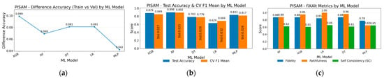
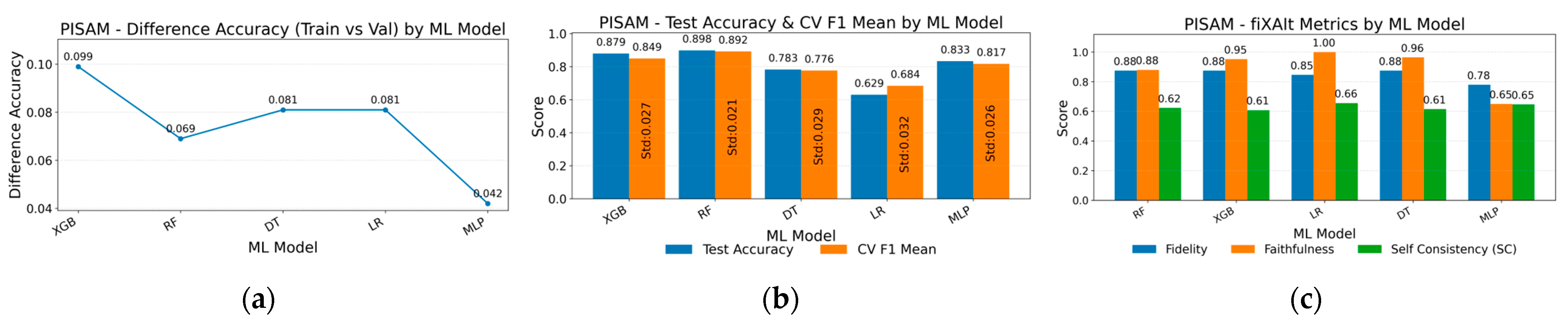
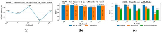
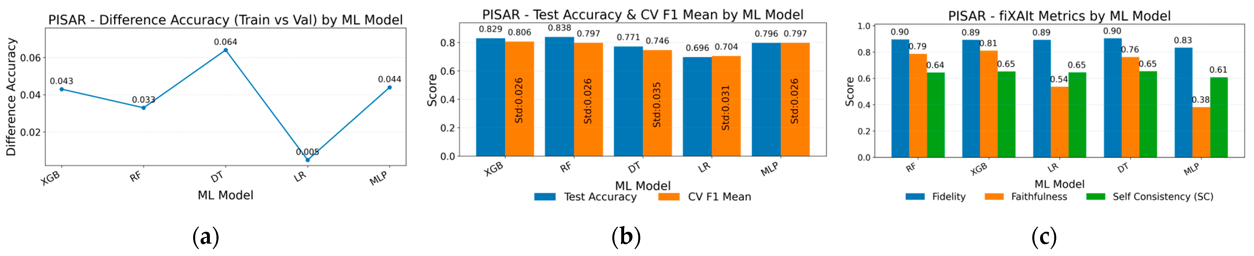
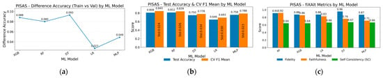
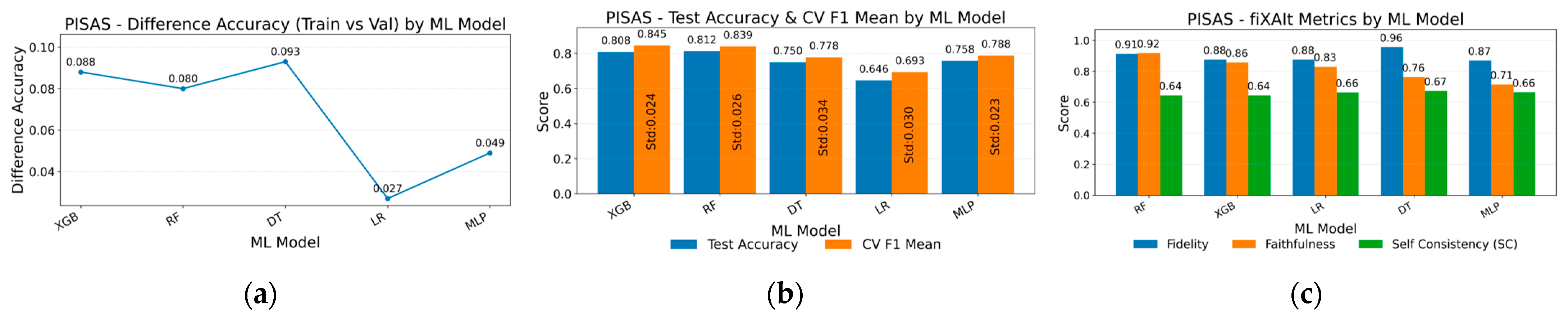
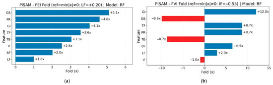
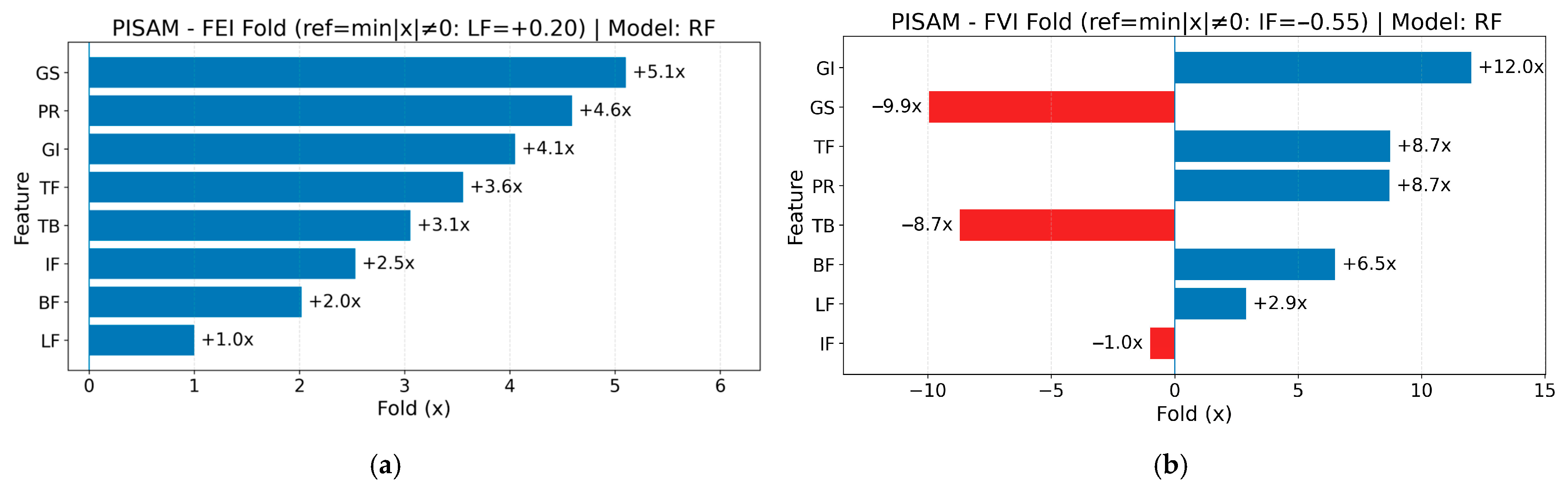
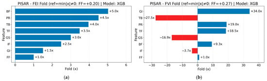
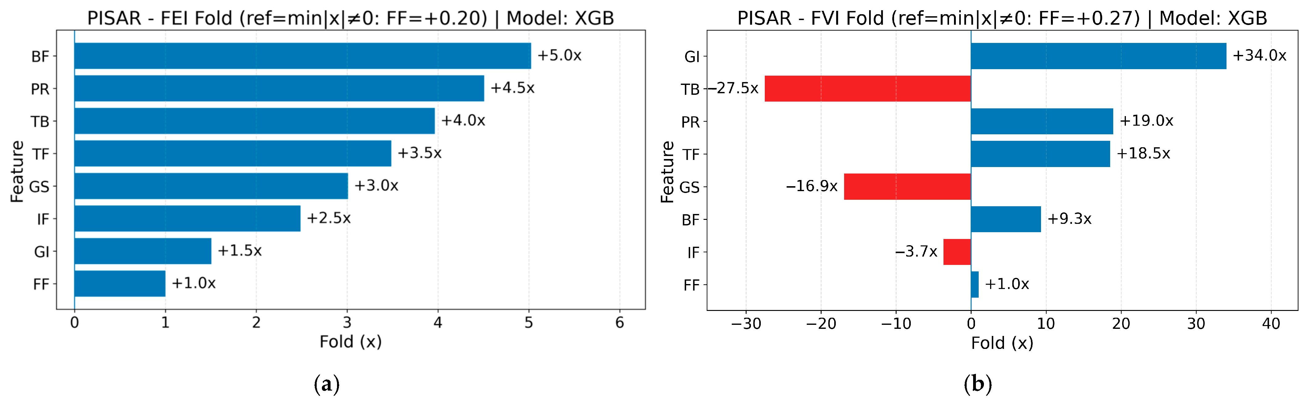
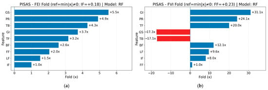
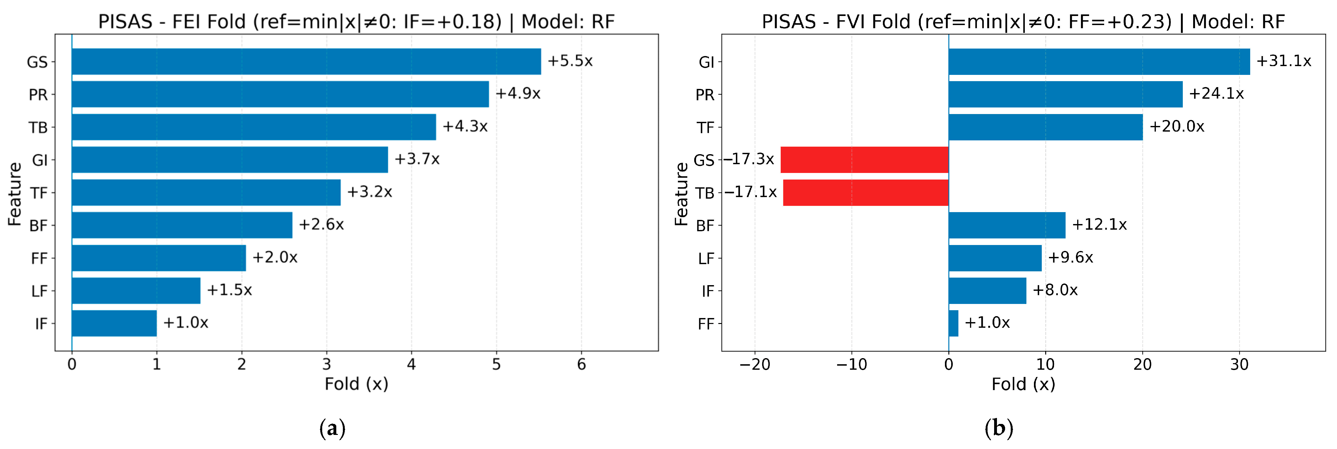
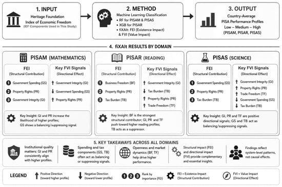
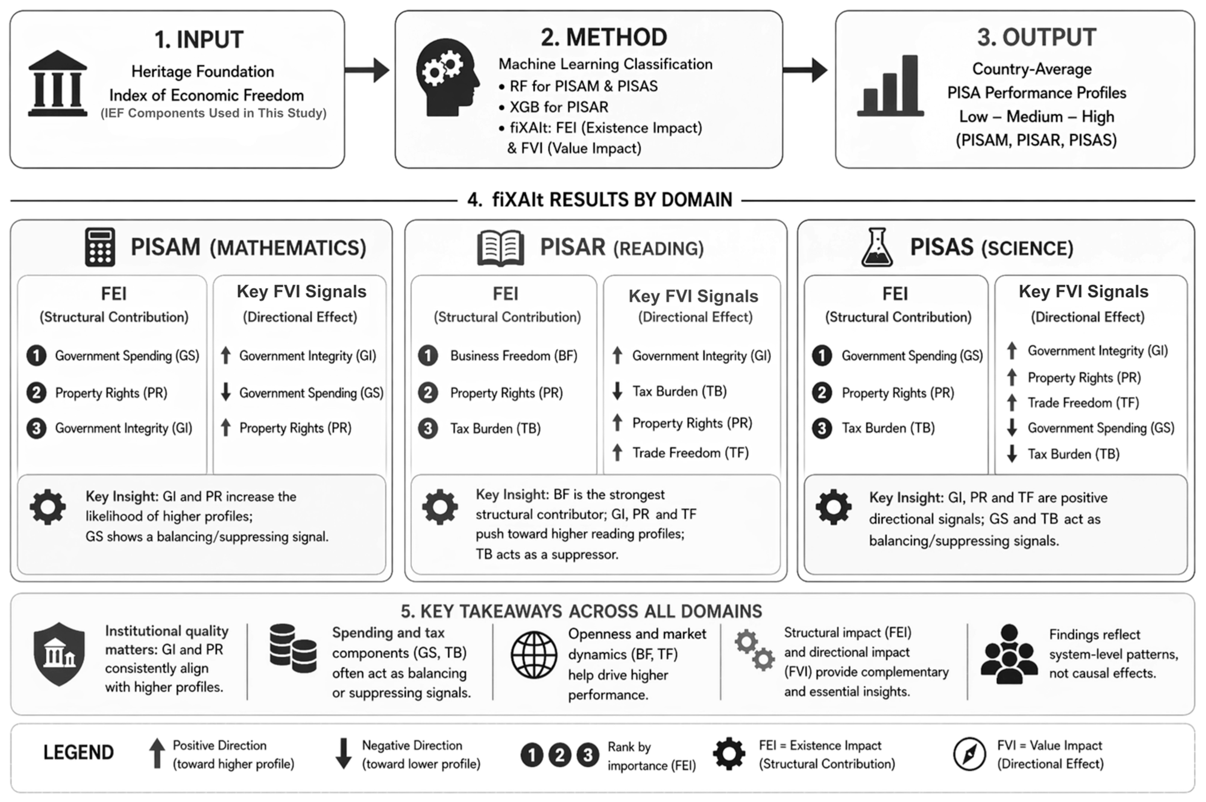

Disclaimer/Publisher’s Note: The statements, opinions and data contained in all publications are solely those of the individual author(s) and contributor(s) and not of MDPI and/or the editor(s). MDPI and/or the editor(s) disclaim responsibility for any injury to people or property resulting from any ideas, methods, instructions or products referred to in the content. |
© 2026 by the authors. Licensee MDPI, Basel, Switzerland. This article is an open access article distributed under the terms and conditions of the Creative Commons Attribution (CC BY) license.