


Abstract
Storage location assignment in automated warehouses strongly affects order-processing efficiency. Existing co-occurrence-based approaches often rely on pointwise mutual information (PMI) statistics or direct frequency co-occurrence. This paper compares two deliberately chosen representation families for storage assignment in automated warehouses operated under Multi-Agent Pickup and Delivery (MAPD) constraints: Pointwise Positive PMI (PPPMI), representing direct pairwise co-occurrence, and Latent Dirichlet Allocation (LDA), representing latent-topic smoothing. The purpose is not to benchmark every possible representation space, but to make the pairwise-versus-latent contrast interpretable under a fixed execution pipeline consisting of task construction, visit-order selection, path planning, and collision avoidance. The broader research setting is motivated by real warehouse order data in which SKU co-occurrence structure is present, but such logs mix latent-topic effects, explicit family-based co-occurrence, noise, and demand variation. We therefore use two controlled abstractions of order structure: one generator with latent-topic mixtures and one generator with more direct family co-occurrence. We embed the proposed LDA representation and the PPPMI baseline in constrained-clustering and simulated-annealing placement methods and evaluate them against frequency-based, load-balancing, and random baselines. Evaluation is conducted in a fixed extended MAPD simulator that explicitly models orientation-aware motion, turning costs, service times, dynamic task release, and collision avoidance. In the latent-topic regime, LDA-based methods tended to form the leading group in average finite-horizon makespan, computed over completed combinations of random seeds and operating conditions. In the supplementary direct-co-occurrence condition, PPPMI was competitive in the plain representation comparison, while LDA-driven local search on top of a frequency-based initial layout remained strong. These results do not imply that LDA is universally superior; rather, they indicate that the relative suitability of PPPMI and LDA depends on the order structure and on how the representation interacts with the placement optimizer. The controlled generators are useful for isolating those effects, but they do not replace external validation on real warehouse logs.
1. Introduction
Fulfillment centers are operational nodes within logistics and supply networks, and their efficiency directly influences end-to-end supply-chain performance. Among warehouse processes, order picking is especially critical because it aggregates the items required for each customer order and accounts for a large share of processing time and operating cost [1,2,3]. The growth of e-commerce has increased both order volume and demand variability, which in turn has strengthened the need for highly automated warehouse operations capable of handling frequent and short-lead-time outbound requests. Recent application-oriented studies of robotic picking and robotic warehousing similarly emphasize that algorithm design must be evaluated together with the operational environment in which humans, robots, and inventory decisions interact [4,5].
Against this background, goods-to-person automated warehouses such as Robotic Mobile Fulfillment Systems (RMFSs) have attracted considerable attention [3,6]. In RMFS-like systems, robots transport shelves or pods to picking stations, where workers or automated equipment retrieve the requested items. This architecture reduces worker travel and improves responsiveness, but it also creates persistent multi-agent interference because many robots move continuously in a shared space. Path conflicts, aisle congestion, and waiting times can therefore dominate operational performance. Such settings are naturally related to Multi-Agent Pickup and Delivery (MAPD), where multiple agents repeatedly serve transport requests that arrive over time [7,8,9].
However, warehouse performance is not determined only by online task allocation and collision-free path planning. Storage location assignment, namely, the decision of which storage slot holds each SKU, also has a large effect on robot travel distance, congestion, service time, and finite-horizon completion time. Placing high-frequency SKUs in accessible positions or locating SKUs that are frequently requested together near one another can directly improve outbound efficiency. Accordingly, storage location assignment has long been studied as the Storage Location Assignment Problem (SLAP) [1,10,11,12].
Prior SLAP studies have considered frequency-based, class-based, distance-based, and load-balancing policies, as well as approaches that exploit co-occurrence among products requested in the same order [13,14]. Co-occurrence-based placement is attractive because it can reflect order structure that is difficult to capture through single-SKU frequency alone. At the same time, the co-occurrence representations used so far have mostly been based on pointwise mutual information (PMI) variants, direct pair counts, or rule-based associations. The use of latent topic representations, which are standard in text mining, remains underexplored for warehouse storage assignment.
This paper therefore studies Latent Dirichlet Allocation (LDA) as a co-occurrence representation for storage assignment in automated warehouses and compares it with Pointwise Positive PMI (PPPMI). Although LDA was originally proposed as a probabilistic model for extracting latent topic structure from document collections [15,16], it can also be applied to order data by treating each order as a “document” and each SKU as a “word”. Under this interpretation, LDA may capture smoothed latent relations among SKUs that differ from the more literal pairwise associations emphasized by PMI-based features.
The comparison is intentionally narrow. Our purpose is not to benchmark every available representation family, but to contrast two interpretable modeling choices under the same execution pipeline, by which we mean the fixed sequence of task construction, visit-order selection, motion planning, reservation handling, and collision avoidance used to execute a placement: PPPMI as a representation of directly observed pairwise co-occurrence, and LDA as a representation that smooths co-occurrence through latent topics. Alternatives such as nonnegative matrix factorization (NMF) [17], correlated topic models (CTM) [18], and BERT-based embeddings [19] are also plausible candidates, but they are outside the present scope and remain for future work.
The broader research setting is motivated by practical warehouse order data, in which SKU co-occurrence structure is present. However, real logs can mix latent topic-like regularities, explicit family-based co-occurrence, noise, and demand variation. If all of these effects are left entangled, a PPPMI-versus-LDA difference is difficult to interpret. For that reason, this journal version uses two controlled order generators: a latent-mixture generator (topic) and a direct family-co-occurrence generator (basket). These generators should be read as controlled abstractions of co-occurrence patterns suggested by real orders, not as a substitute for eventual validation on real warehouse logs.
Our goal is not to claim that LDA is always better than PPPMI. Rather, we ask when a latent-topic representation is better matched to the order structure and whether that representational fit propagates to execution performance when the only experimental factor varied is the storage assignment policy. To keep the comparison interpretable, the main experiment uses orders with explicit latent topic structure, and a supplementary direct-co-occurrence condition (basket) checks how the conclusions change when co-occurrence is dominated more directly by explicit pairwise association. Concretely, we compare PPPMI and LDA as co-occurrence representations, embed them in both clustering-style and local-search-style placement methods, and compare them with classical baselines that do not use co-occurrence information. Evaluation is performed in an extended MAPD simulator with a fixed planner that includes orientation-aware motion, turning costs, loading/unloading service times, and collision avoidance. This isolates the impact of storage assignment under a realistic execution pipeline rather than under a purely geometric distance surrogate.
The main questions addressed in this paper are as follows. First, under order streams with latent-topic structure, is LDA more effective than PPPMI as a co-occurrence representation for storage assignment? Second, is the effect of the representation consistent across clustering-style and local-search-style placement methods, or does it depend on the interaction with the initial solution, the operating conditions, and the order structure itself?
The contributions of this paper are threefold:
- Methodological contribution: we evaluate storage assignment in the context of extended MAPD with a fixed planner that explicitly models orientation-aware motion, turning costs, service times, and collision avoidance, thereby providing a framework for comparing placement policies through execution performance in automated warehouses.
- Positioning and comparison contribution: we frame the study as an interpretable comparison between PPPMI as a direct pairwise representation and LDA as a latent smoothing representation, and complement the main topic-structured condition with a basket ablation so that the representation effect can be interpreted in terms of order structure rather than treated as a generic benchmark ranking.
- Empirical contribution: in the controlled topic-structured regime, LDA-based methods tended to form the leading group in mean makespan, whereas in the direct-co-occurrence condition (basket) PPPMI became competitive in the plain representation comparison; thus the results point to structure-dependent suitability of PPPMI versus LDA rather than to universal dominance of either representation.
Note on Prior Publication
Parts of this study build on our PAAMS 2025 conference paper [20]. The conference version reported an earlier storage-assignment study under a simpler execution setting, where immediate task assignment was handled by a greedy strategy and the empirical scope was more limited. The present journal manuscript substantially extends that work by replacing the earlier execution setting with a more realistic warehouse-oriented execution pipeline, referred to here as SHARP [21], built on the Anytime Multi-Task MAPD simulator framework [22]. Here, the execution pipeline denotes the complete fixed implementation used during evaluation, including task construction, visit-order generation, orientation-aware path search, reservation-table collision avoidance, and service-time handling. It also broadens the evaluation to multiple layouts, load conditions, goal policies, noise levels, and a larger comparison set, and it adds the PPPMI-versus-LDA analysis, the initial-solution ablations, and the supplementary order-structure experiments.
2. Related Work
This section reviews prior work on MAPD, SLAP, and co-occurrence modeling from the viewpoint most relevant to this paper: how to evaluate storage assignment while accounting for multi-agent interference during execution.
2.1. Multi-Agent Pickup and Delivery
MAPD studies how multiple agents should repeatedly serve transport tasks while maintaining collision-free motion. Representative methods include Token Passing and related schemes, and more recent work has improved scalability and congestion handling in large systems [6,7,8,9,23,24,25]. Most of this literature assumes that pickup locations are already given and focuses on online assignment and planning rather than on how storage locations should be designed. An exception more closely related to our setting is the work of Hattori et al. [14], which reported MAPD execution improvements through capacity-constrained clustering with co-occurrence information. Our study follows this direction by keeping the planner fixed and comparing storage assignment designs instead.
2.2. Storage Location Assignment Problem
The SLAP literature covers classical policies such as random storage, frequency-based storage, and class-based storage, as well as metaheuristic optimization for assignment refinement [1,2,11,26]. Closest to this paper are correlated-storage approaches that place related SKUs near each other by exploiting order-level associations [12,13,27,28]. Recent practical robotic-warehousing studies also show the importance of evaluating inventory, picking, and robot-execution decisions in an integrated operational setting rather than as isolated geometric subproblems [4,5]. However, many SLAP studies still evaluate policies mainly through travel distance for one or a few pickers. A comparatively limited number of studies incorporate MAPD-specific interference, collision avoidance, and shared-space congestion directly into the evaluation loop.
2.3. Co-Occurrence Analysis for Order Data
Pointwise mutual information (PMI), positive PMI (PPMI), and frequent-itemset mining are widely used to represent correlations in transactional data [29,30,31]. A PMI-derived representation describes each SKU by how strongly it co-occurs with the other SKUs in the order history. In this paper, PPPMI denotes the nonnegative SKU-feature matrix obtained from positive PMI with smoothing, so it functions as a direct feature representation of observed pairwise co-occurrence. Hattori et al. [14] used PMI-based similarity features in combination with capacity-constrained clustering and demonstrated placement improvements in automated warehouse settings. At the same time, pairwise methods rely heavily on directly observed pairs and therefore leave open the question of how to smooth sparse or unobserved co-occurrences.
2.4. Latent Dirichlet Allocation
LDA [15,16] is a generative model that represents discrete observations as mixtures of latent topics. It has also been applied to short transactional data such as purchase histories and market baskets [32,33,34]. The appeal of LDA in our setting is that it can represent not only direct pairwise co-occurrence but also higher-order latent structure shared across several SKUs. Nevertheless, its robustness on short orders and, more importantly, its contribution to actual storage-assignment performance in automated warehouses remain insufficiently understood.
2.5. Research Gap and Positioning
The literature therefore leaves three related gaps. First, MAPD research and SLAP research are still largely separate, and only a limited number of studies evaluate the interaction between placement design and multi-agent interference in a unified experimental setting that resembles practical robotized warehouses. Second, PPPMI has been tested as a co-occurrence representation for storage assignment, but the conditions under which latent representations such as LDA are advantageous are not yet clear. Answering that question requires controlling the order structure; otherwise an observed PPPMI-versus-LDA difference is hard to interpret. Third, the goal of the present paper is not an exhaustive benchmark across every modern representation family. Alternatives such as NMF [17], CTM [18], and BERT-based embeddings [19] are also plausible candidates, but including all of them would blur the more interpretable question addressed here: how a direct pairwise representation compares with a latent smoothing representation under the same execution pipeline. This paper therefore addresses the first two gaps by positioning itself as a deliberately controlled comparison between PPPMI and LDA within a shared extended MAPD simulator while disentangling the roles of the representation, the initial solution, local search, and order-generation structure. Broader representation benchmarking is left for future work.
3. Problem Setting
3.1. Evaluation Setting as an Extended MAPD Problem
We treat automated warehouse operation with storage assignment as an extended MAPD problem. Let the warehouse environment be
where is the movement graph induced by the warehouse grid and is the set of agents. Let denote the order stream, the set of SKUs, and the set of storage slots. The storage assignment is represented by
Figure 1 illustrates the warehouse environment used by the simulator on the well-formed layout. The traversable cells form
and edges in connect adjacent traversable cells. Because each has multiple shelf levels h, an assignment specifies both the access cell and the shelf level behind that cell.
Figure 1.
Schematic warehouse environment based on the simulator’s well-formed layout. The movement graph is constructed from traversable cells, and the storage slots are defined as , namely, a pair of a pick-access cell and a shelf level. The lower-left panel gives the legend for the cell symbols X, O, R, P, U, L, and S, and the lower-right panel illustrates how shelf levels h are attached behind an example P cell v.
The joint optimization problem of agent execution and storage assignment can then be written as
where maps the order stream and a storage assignment to an MAPD task sequence and denotes makespan. In this paper, makespan means the completion time of the last order request released within the finite evaluation horizon, that is, the elapsed time until all released orders have been processed. Jointly optimizing online MAPD decisions and storage assignment is computationally difficult, so in this paper we fix the agent policy and compare only the storage assignment:
Equations (1) and (2) distinguish the full joint problem from the fixed-planner storage-assignment subproblem addressed here. This lets us compare placement methods through the execution performance they induce under a realistic, fixed planner. Because real warehouses operate continuously, makespan is not used here as a standalone long-run operational KPI. It is a finite-horizon dynamic-simulation metric: orders are released during the evaluation horizon, the simulator continues until all released order requests are completed or the maximum simulation length is reached, and the reported makespan is the last completion time. The mean makespan reported later is the arithmetic mean of these run-level makespans over the completed combinations of random seeds and operating conditions.
3.2. Warehouse Layout and Storage Slots
The warehouse is represented as a rectangular grid. Table 1 summarizes the meaning of each cell type. Traversable cells are divided into , , , , and , and the set of outbound goal cells is denoted by . SKU items are stored in racks behind P cells, and each P location has H shelf levels. The set of storage slots is therefore
The level index h distinguishes storage positions vertically, while robot motion is still executed on the two-dimensional grid.
Table 1.
Meaning of the grid-cell symbols.
The simulator contains at least two layout types:
- Non-well-formed layout: shared aisles are narrow and passing opportunities are limited, so congestion is likely to cause head-on blocking.
- Well-formed layout: shared aisles are wide and intersections permit easier avoidance behavior, making it possible to test whether a placement method remains effective under more permissive geometry.
Our use of the term “well-formed” follows the well-formed infrastructure condition of Čap et al. [35]: any pair of endpoints is connected by a path that avoids other endpoints sufficiently so that robots resting at endpoints do not completely block the system. The non-well-formed layout does not satisfy this condition and is instantiated here as a narrow-aisle setting with concentrated interference. By using both layout types, we can test whether the placement effects generalize beyond one specific warehouse geometry.
3.3. Order Generation and Order-Request Construction
Orders are generated at discrete timesteps . At each timestep, an order is generated with probability . Order size is drawn from
and the main experiments use and .
In the experimental setting used here, the SKU catalog contains items partitioned into multiple product families, meaning groups of related SKUs that tend to appear in similar order contexts. Within each family, core items act as the central representative SKUs of the group, halo items are neighboring SKUs that are somewhat less central but still likely to be chosen together with the core items, and weak bridge relations connect neighboring families. This family structure is shared by the latent-structure generator used in the main experiments (topic) and by the direct-co-occurrence generator used in Appendix A.4 (basket).
The order generators are used because the purpose of this paper is to compare co-occurrence representations under controlled structure rather than on a single mixed dataset. The broader research setting is informed by real warehouse order data, where SKU co-occurrence structure is present, but such logs can combine latent mixture structure, explicit family-based co-occurrence, noise, and demand variation. If training and evaluation orders mix several mechanisms simultaneously, a PPPMI-versus-LDA difference is difficult to interpret. The main experiment therefore uses the latent-structure generator (topic) as a controlled regime for testing a latent representation, while Appendix A.4 uses the direct-co-occurrence generator (basket) as a counterpoint in which explicit family-level association is stronger and PMI-based statistics may be better matched. The generators are thus intended as controlled abstractions of co-occurrence structure suggested by real orders, not as toy settings and not as replacements for final validation on real warehouse logs. In particular, they let us vary whether the order stream is driven more by latent topic mixtures or by more explicit within-group co-occurrence, together with order size, arrival rate, and co-occurrence degradation through noise, while keeping the SKU catalog, planner, and warehouse layouts fixed.
Under the latent-structure generator (topic), each order is sampled from a topic–SKU distribution Φ that is consistent with the family structure:
Here, is the order-level topic mixture for order t, is the topic assigned to the n-th SKU token in that order, is the sampled SKU, and Φ is the topic–SKU distribution. In the main experiment, we fix . Hence each order is generated as a mixture of latent topics. This provides a controlled condition under which we can test whether a latent representation yields an execution advantage when the order stream truly contains latent mixture structure. The direct-co-occurrence generator (basket) is treated as an order-data ablation in Appendix A.4. Both generators include a noise rate , which replaces a fraction of sampled SKUs with other SKUs in order to control co-occurrence degradation.
Training and evaluation order streams are generated independently and are then converted into simulator order requests according to the storage assignment p. Each order request is simply the simulator representation of one outbound order: it specifies when the order appears, which pick-access cells must be visited, and which unloading destination cell must be reached. For an order , the corresponding order request is written as
where is the release timestep, is the set of rack-front access cells corresponding to the ordered SKUs under assignment p, and is the outbound goal. The word “goal” is used in the MAPD sense of a destination cell for unloading, not as a performance objective. We use two goal policies. Under random, is sampled uniformly from the outbound goals. Under nearest, the unloading cell minimizing the total travel distance from the ordered SKU access cells is selected. Consistent with the shared evaluation settings, the reported experiments use fixed service times of 5 for picking, unloading, and loading; in particular, the picking dwell time is 5 for every SKU.
3.4. Agent Motion Model and Operational Costs
The state of each agent a is
that is, the simulator tracks both position and orientation. This is necessary because rack access direction and turning time are modeled explicitly.
The primitive actions are forward motion, rotation, and waiting. Their unit costs are
The default value is , so turning is more expensive than one straight step. Hence the evaluation depends on orientation-aware travel cost rather than only on Manhattan distance.
Service actions also incur explicit dwell times. Picking SKU c requires
unloading at an outbound location requires
and loading at an inbound location requires
Thus, all service times used in the reported experiments are fixed at 5. Modeling turning, picking, unloading, and loading separately prevents the placement evaluation from collapsing to a pure shortest-distance objective.
The MAPD execution constraints are:
- No two agents may occupy the same cell at the same time (no vertex conflict).
- No two agents may swap cells across consecutive timesteps (no edge-swap conflict).
- A home S cell assigned to another agent is not traversable and remains exclusive to its owner.
- Cells P, U, and L remain reserved during service dwell times.
3.5. Fixed Planner: Base Simulator and SHARP Execution Layer
The evaluation pipeline in this paper uses the simulator setting of Anytime Multi-Task MAPD under energy constraint [22] as its base framework. On top of that base framework, we use a warehouse-oriented execution layer, referred to here as SHARP [21]. In other words, Anytime Multi-Task MAPD is the underlying simulator setting, whereas SHARP is the stronger execution model used in this study for placement evaluation. The purpose of the present work is not to improve task allocation or path planning themselves, but to compare storage assignment under a common execution pipeline. For this reason, the simulator uses the same deterministic task-release stream and the same fixed execution rules for every placement method. When an agent becomes available, the fixed task-assignment rule selects the next released order request according to the base simulator configuration; the visit-order module then enumerates candidate orders for visiting the pick-access cells in that request, and the planner executes the selected order while respecting the reservation table. Relative to the simpler conference setting that used greedy immediate-task assignment, SHARP retains the same base simulator configuration while adding the warehouse-specific execution rules needed in this study, such as orientation-aware motion costs, service times at P/U/L cells, and route execution that can insert waiting or detours through reservation-aware planning. All of these assignment and planning choices are fixed across methods; no storage-assignment method is allowed to change them.
The planning layer used in the experiments consists of candidate visit-order generation within a task, orientation-aware static A* cost computation [36], and collision avoidance through Safe Interval Path Planning (SIPP) with a reservation table [37]. In single-agent planning, both position and orientation are part of the state; forward cost is 1 and turn cost is . When the agent services P, U, or L, the corresponding cell remains occupied for the full service duration. SIPP constructs safe intervals from the reservation table and inserts only the waiting needed to avoid vertex and edge-swap conflicts. This gives a realistic but fixed planner with which to compare storage assignments while keeping the underlying simulator consistent across methods.
For reproducibility, the simulation loop is as follows. At each timestep, newly released orders are converted to order requests according to the current storage assignment. When an agent is available, the fixed assignment rule selects one released order request; the visit-order module enumerates candidate orders of the required pick-access cells; the orientation-aware A* module computes static route costs for those candidates; and SIPP generates a reservation-table-consistent route for the selected sequence. The agent then executes forward moves, rotations, waits, and service dwell actions, while occupied cells are recorded in the reservation table. A run terminates when all order requests released within the finite evaluation horizon have been completed or when the maximum simulation length is reached. This loop is identical for all storage-assignment methods, so the reported differences arise from the placement p rather than from changes in task allocation or path planning.
3.6. Fixed Elements in the Comparison Design
The only experimental factor varied in this paper is the storage assignment method. The following components are fixed across all compared conditions:
- the order-generation rules and random-seed handling;
- the goal policy (random or nearest);
- the visit-order enumerator within each order request;
- the orientation-aware A* and reservation-table SIPP planner;
- the turning cost and all service-time parameters.
Consequently, performance differences in the experiments indicate how strongly changes in SKU placement propagate to MAPD execution under realistic costs and collision avoidance.
4. Method
This section formulates the storage assignment methods. Let the SKU set be and the training-order set be . Each order is treated as a set of SKUs, and indicates whether SKU i appears in order d. Let be the set of storage slots and the set of outbound goals. Each slot has position , shelf level , and a fixed goal-zone assignment
where is randomly generated before the experiments and then shared across all compared methods. We write for the zone corresponding to goal u and for its capacity. The storage assignment is a bijection.
We compare the methods ck-pmi, ck-lda, sa-pmi, sa-lda, pmi-frequency-nearest, and lda-frequency-nearest alongside three classical baselines. Table 2 summarizes the compared methods and the intended comparison axes.
Table 2.
Compared methods and their roles in the comparison.
4.1. Proxy Objective
The ultimate objective is to improve makespan under the fixed planner. Directly searching over storage assignments using simulated makespan as the objective is computationally expensive, because each candidate assignment p requires a full dynamic MAPD simulation with task releases, service times, and reservation-table collision avoidance. We therefore introduce a surrogate that encourages SKUs that co-occur frequently to be placed near each other. The surrogate is based on the following operational rationale rather than on a formal optimality proof. If SKUs that tend to appear in the same order are assigned to nearby access cells, then the set of pick cells visited within one order becomes less spatially dispersed. Under the fixed execution policy, lower dispersion tends to shorten between-pick travel, reduce the time for which agents occupy productive aisle segments near those picks, and thereby reduce reservation conflicts and waiting cascades. The resulting placement is therefore expected to reduce both per-order service time and congestion-induced delay, which moves makespan in the favorable direction.
For slots , define
where controls the contribution of shelf-height difference. Under assignment , the slot distance between SKUs i and j is
Let be a co-occurrence weight representing how strongly SKUs i and j tend to be requested together. We then consider the weighted distance sum
This quantity measures the average spatial dispersion of strongly co-occurring SKU pairs and serves as a proxy for how spread out the visited pick cells of one order will be. Equations (3) and (4) define the distance and weighted-dispersion terms used by this surrogate. Reducing it should shorten intra-order movement and narrow the temporal occupancy window created by one task.
If the per-order processing time can be approximated by a sum of fixed processing cost, within-order movement, and congestion delay proportional to that movement, then
Here, summarizes the sensitivity of within-order travel time to the weighted dispersion , while summarizes the sensitivity of congestion delay to the same travel-related occupancy. Equation (5) is not claimed as a rigorous bound because actual makespan also depends on task interleaving, route conflicts, and planner decisions. Rather, it formalizes the directional argument above: concentrating within-order SKU locations reduces travel and aisle occupancy, and lower occupancy tends to reduce MAPD contention and hence makespan. Section 6.5 later checks this claim empirically by comparing the surrogate with measured mean makespan. The methods below therefore derive SKU embeddings for clustering and pair weights for simulated annealing from PMI- and LDA-based co-occurrence representations.
4.2. Co-Occurrence Representations (PMI/LDA)
Define SKU order frequency and pairwise co-occurrence count by
PMI-based statistics are computed from set-based frequencies, that is, repeated appearances of the same SKU within one order are collapsed.
4.2.1. PPPMI Representation
For PMI-based methods, we first compute
We smooth the context-side marginal as
which mitigates the tendency of raw PMI to overweight low-frequency events and follows the context-distribution smoothing practice shown to be effective in distributional similarity and PPMI-based representations [38]. The asymmetric PMI is
and the symmetric positive PMI matrix is defined by
Equation (6) defines the PPPMI value used as the direct pairwise co-occurrence representation. The PMI embedding of SKU i is the row vector
4.2.2. LDA Representation
For LDA-based methods, each order is treated as a document and each SKU as a word. We train LDA with K topics, Dirichlet priors
and collapsed Gibbs sampling. These hyperparameters are fixed across all conditions; sensitivity analysis for them is beyond the scope of this paper. The value encourages each order to concentrate on a small number of topics, while keeps topic–SKU distributions sparse enough to preserve family-level structure without assigning zero probability to rare SKUs. Thus, the LDA parameters are used to obtain a stable latent representation for the placement comparison rather than to tune the simulator outcome. For the nth token in document d taking SKU i, the topic-assignment update is
where is the number of times topic k is assigned in document d, is the number of times SKU i is assigned to topic k, and .
After training, the topic-word distribution and topic prior are estimated as
The SKU embedding used in CK-style clustering is the posterior topic distribution of SKU i,
For the simulated-annealing objective, we also construct the shared-topic pair matrix
Equations (7), (8), and (9) respectively define the Gibbs update, SKU embedding, and shared-topic pair matrix used by the LDA-based methods.
Representational Difference Between PMI and LDA
PMI directly scores observed pairwise co-occurrence using only and the marginals . Unobserved pairs therefore receive no positive evidence. By contrast, LDA infers higher-order latent structure through a shared topic variable. Even when direct co-occurrence is sparse, two SKUs may still obtain similar embeddings or positive pair weight if they are likely under the same topic. The PMI-versus-LDA comparison in this paper can thus be interpreted as a comparison between faithful use of observed pair co-occurrence and smoothed latent-topic modeling.
4.3. Baseline Placement Methods
We first compare three classical baselines: random, frequency-nearest, and balance. These methods are easy to interpret and represent three different design principles without explicit co-occurrence modeling: random placement, placing high-frequency SKUs near goals, and balancing load across zones.
4.3.1. Random
The random method ignores co-occurrence entirely. It shuffles the SKU set and the slot set independently and matches them in order. Equivalently,
where is the set of all bijections from to . This provides a neutral baseline against which the benefit of co-occurrence-aware methods can be assessed.
4.3.2. Frequency-Nearest
The frequency-nearest baseline sorts SKUs by descending order frequency and assigns them to slots sorted by increasing average distance to the outbound goals. Frequent SKUs are therefore prioritized for easy-to-access slots. This is a classical turnover-based storage policy that does not use co-occurrence information.
4.3.3. Balance
The balance baseline aims to distribute the number of SKUs approximately evenly across goal zones. After shuffling the SKUs, it assigns them to zones in round-robin order. The within-zone order remains random, so neither frequency nor co-occurrence is used.
4.4. CK-Style Placement
CK-Style Capacity-Constrained Clustering
The ck-* initial solutions are generated by a CK-style capacity-constrained clustering heuristic. The input is an SKU embedding and a frequency value for each SKU. First, the embeddings are normalized as
Next, seeds are chosen by
and, for ,
The first factor prefers high-frequency SKUs, and the second factor discourages selecting seeds too similar to earlier ones. The term prevents the frequency factor from becoming zero for tail SKUs, so seed selection remains jointly influenced by frequency and representational diversity even for rarely ordered items.
Each zone is then paired with one seed, and SKUs are processed in descending frequency order. An SKU is assigned to the feasible zone with remaining capacity that maximizes
breaking ties in favor of the zone with lower fill ratio , where is the current set of SKUs assigned to zone u and is its capacity. Thus, when two zones are equally similar for a given SKU, the less-filled zone is preferred. For the set assigned to zone u, we compute the centroid
then sort SKUs within the zone so that high-frequency SKUs similar to the centroid appear earlier. This ordering is mapped to the slots in sorted by proximity to goal u. For example, suppose there are two zones and with capacity 2 each and three SKUs processed in descending frequency order. If and become the two seeds, then is assigned to the zone whose seed has the larger cosine similarity to ; if the similarities tie, the algorithm chooses the zone with the smaller current fill ratio. After zone membership is fixed, the SKUs inside each zone are ordered using frequency and centroid similarity and then mapped to the nearer slots of that zone.
- ck-pmi
ck-pmi uses in Equations (10) and (11). Hence each row of the PPPMI matrix is treated as the direct co-occurrence profile of a SKU, and SKUs with similar profiles are clustered into the same zone.
- ck-lda
ck-lda uses instead. It therefore groups SKUs according to similarity in posterior topic distribution rather than direct pairwise co-occurrence. The comparison between ck-pmi and ck-lda isolates the effect of the SKU representation under the same clustering mechanism.
4.5. SA-Style Placement
4.5.1. Objective Function for Simulated Annealing
For SA-style methods, the slot distance in Equation (3) is transformed into a slot closeness score
Equation (12) is then combined with the pair-weight definitions below, and we use . To emphasize frequent SKUs without letting frequency dominate the co-occurrence signal, we normalize frequency by
The PMI-based pair weight is
and the LDA-based pair weight is
The cosine-similarity term in Equation (13) complements the direct PMI entry with neighborhood similarity in the PPPMI embedding space, while the factor upweights pairs that are both related and operationally frequent without letting frequency alone dominate the score. Equation (14) plays the analogous role for LDA by weighting pairs according to their shared latent-topic mass. For an arbitrary pair-weight matrix W, the objective is
Simulated annealing maximizes Equation (15), which is consistent with the surrogate principle of placing strongly related SKU pairs in nearby slots.
4.5.2. Neighborhood Search and Temperature Schedule
A neighborhood move swaps two slots. First, SKU i is selected according to
where smooths the selection so that low-frequency SKUs are still explored. The slot containing SKU i is then swapped with a uniformly sampled slot from the remainder. Accordingly, the proposal distribution is generated by a frequency-biased first choice followed by uniform partner selection over the remaining slots. The goal is heuristic search rather than unbiased sampling, so frequently requested SKUs are revisited more often while every remaining slot can still appear as the swap partner. Let be the difference between the new and old objective values. The acceptance probability is
The temperature follows geometric cooling:
Equations (16) and (17) define the acceptance and cooling rules used by the SA variants. where is the 80th percentile of over pre-sampled worsening swaps and
Here, controls the initial willingness to accept worsening swaps, sets the minimum exploration temperature, and is the total number of swap iterations in the schedule. This configuration is shared across all SA-based comparisons.
- sa-pmi
sa-pmi uses as the initial solution and optimizes Equation (15) with . The difference between ck-pmi and sa-pmi therefore isolates the additional effect of swap-based local search when the PMI representation is fixed.
- sa-lda
sa-lda uses and optimizes . Comparing ck-lda with sa-lda shows whether clustering alone is sufficient under the LDA representation or whether heuristic local search adds value.
- lda-frequency-nearest
lda-frequency-nearest uses as its initial solution and then optimizes the LDA objective . Relative to frequency-nearest, it measures the benefit of adding LDA-driven local search on top of a classical turnover-based layout. Relative to sa-lda, it measures the effect of the initial solution when the LDA objective is held fixed.
- pmi-frequency-nearest
pmi-frequency-nearest also starts from , but it optimizes instead. It is included to test whether the dependence on the initial solution observed for LDA is specific to LDA or also appears with PMI.
- Intent of the Comparison Design
The comparison design in Table 2 serves three purposes. Comparison with classical baselines tests whether co-occurrence information is useful at all. Comparison between ck-pmi/ck-lda and between sa-pmi/sa-lda isolates the representational effect of PPPMI versus LDA under matched construction mechanisms. Finally, comparison with pmi-frequency-nearest and lda-frequency-nearest reveals whether performance depends on the interaction between the co-occurrence representation and the initial solution.
5. Experimental Design
5.1. Research Objective and Questions
The experiments replace only the storage assignment p while keeping the planning pipeline fixed. The purpose is to identify how differences in co-occurrence representation and placement construction affect execution performance. The central question is not whether one representation universally dominates the other, but whether PPPMI and LDA behave differently when the order structure is controlled and the only experimental factor varied is the storage assignment method. We formulate the following research questions:
- RQ1: Do co-occurrence-aware placements outperform baselines that do not use co-occurrence information?
- RQ2: Which co-occurrence representation is more effective, PPPMI or LDA?
- RQ3: How do placement construction style and initial solution affect the observed gains?
- RQ4: How stable are the above tendencies under changes in goal policy, noise rate, number of agents, order arrival rate, and warehouse layout?
- RQ5: To what extent do the findings remain valid under different order structures and different numbers of LDA topics?
5.2. Compared Methods and Comparison Intent
The compared methods are random, balance, frequency-nearest, ck-pmi, ck-lda, sa-pmi, sa-lda, pmi-frequency-nearest, and lda-frequency-nearest. These methods are organized around three comparison axes:
- Comparison against non-co-occurrence baselines:random, balance, and frequency-nearest serve as reference points for testing whether using co-occurrence itself improves makespan.
- Comparison of co-occurrence representations:ck-pmi versus ck-lda and sa-pmi versus sa-lda compare PPPMI and LDA under matched construction mechanisms.
- Comparison of construction style and initial solution:ck-lda versus sa-lda evaluates the added effect of local search, and pmi-frequency-nearest and lda-frequency-nearest test how co-occurrence-based local search interacts with a frequency-based initial solution.
For LDA-based methods, we use topics. These two values were selected as moderate topic granularities for a 600-SKU catalog: provides coarse latent families, whereas allows finer subdivisions without making the representation comparison an extensive hyperparameter search. We report both values in the main results, but because this is only a two-point comparison, we treat topic-number effects conservatively and return to them only in the overall discussion. This experimental design should therefore be read as a controlled comparison, not as a claim of exhaustive benchmarking over all representation families or all real-world order distributions. The background of the study includes practical order data in which SKU co-occurrence structure is present, but those data mix several mechanisms that are difficult to disentangle directly. The topic and basket generators are used here to separate latent-topic-like and explicit family-based co-occurrence patterns so that the relative behavior of PPPMI and LDA can be interpreted more clearly. Final external validation on real warehouse logs remains future work.
5.3. Evaluation Environment and Metrics
The evaluation fixes the agent policy in the extended MAPD problem defined in Section 3.1 and changes only the storage assignment p. The question is therefore how the overall execution performance of the warehouse changes when only SKU placement is altered under the same robot team and planner configuration. The primary evaluation metric is makespan, namely the completion time of the last order request among those released during the evaluation horizon. The main comparisons in the body text are based on mean makespan, computed as the arithmetic mean over completed run-level simulations for the relevant condition set. For the most important paired comparisons, Appendix A.1 additionally reports exact sign tests, bootstrap 95% confidence intervals, and paired Cohen’s . Table 3 summarizes the shared evaluation settings. Table 4 and Figure 2 summarize and visualize the two warehouse layouts used in the evaluation.
Table 3.
Shared settings in the evaluation environment.
Table 4.
Structural comparison of the evaluation maps.
Figure 2.
The two warehouse layouts used for evaluation. The lower legend summarizes the cell symbols. The non-well-formed map is a narrow-aisle setting with concentrated interference, whereas the well-formed map offers more room for detours and avoidance maneuvers. (a) Non-well-formed layout with narrow rack gaps and limited cross-aisle freedom. (b) Well-formed layout with wider horizontal aisles and more room for avoidance.
Both maps have 100 storage access cells. With six shelf levels, this yields 600 storage slots in total. Using both layouts lets us test whether the effect of a placement method is tied to one specific geometry.
5.4. Main Experiment: Orders with Latent Topic Structure
The main experiment uses orders with latent topic structure in both training and evaluation (topic→topic). This is the main test bed for RQ1–RQ4 because it directly examines whether representational differences propagate to makespan when the order stream contains latent topic structure. The purpose of this experiment is not to claim a universal advantage for LDA. Rather, it is to test whether an order stream that truly contains latent mixture structure creates a controlled regime in which LDA is better matched than PPPMI under the fixed execution pipeline.
The varying factors are two maps, two agent counts, two order rates, three noise levels, two goal policies, five training seeds, and ten test seeds. This supports both overall averages across all conditions and condition-wise summaries for goal policy, noise, load, and layout. The most important comparisons are ck-pmi versus ck-lda, sa-pmi versus sa-lda, ck-lda versus sa-lda, and the interaction with the frequency-nearest initial solution through pmi-frequency-nearest and lda-frequency-nearest.
5.5. Supplementary Experiment: Robustness to Order Structure
As a supplementary experiment, we evaluate orders with direct co-occurrence structure in both training and evaluation (basket→basket), where the generator creates strong within-family co-occurrence. This experiment tests whether the main findings persist under an order structure different from the latent-topic setting. Its role is to check whether the main result is merely generator specific or whether some conclusions survive when the order structure is better matched to direct pairwise statistics. The full results are reported in Appendix A.4; the main text discusses only the high-level implications in Section 6.6.
5.6. Supplementary Diagnostic: Correspondence Between the Surrogate and Makespan
Section 4.1 introduced a surrogate based on weighted SKU-pair closeness. As a diagnostic, we examine how well this surrogate aligns with actual makespan in the simulator. The aim is not to re-optimize each method but to visualize whether the design principle of placing co-occurring SKUs nearby corresponds monotonically to execution performance.
For this diagnostic, we fix goal policy=random, order rate 0.20, and noise 0.0, and consider the four combinations of non-well-formed/well-formed and 6/12 agents. For each condition, we use the five training-seed placements generated by the representative methods random, balance, frequency-nearest, ck-pmi, sa-pmi, ck-lda (), and sa-lda (), for a total of 45 points per panel. The horizontal axis is a unified computed from a common with , reconstructed from the same training corpus for all placements. The vertical axis is the mean makespan across the ten test seeds for that placement.
6. Results and Discussion
This section answers the research questions in order. Section 6.1 uses Table 5 to establish the overall main-experiment ranking for RQ1, Section 6.2 and Section 6.3 unpack the representation and construction effects for RQ2–RQ3, and Section 6.4 uses Table 6 to show condition dependence for RQ4. Section 6.5 then uses Figure 3 as a diagnostic for the surrogate in Section 4.1, and Section 6.6 summarizes the robustness check under direct-co-occurrence orders (basket) from Appendix A.4 for RQ5.
Table 5.
Overall mean makespan in the main experiment.
Table 6.
Improvement rates by operating condition in the main experiment (relative to random under the same condition). For readability, we report ck-lda and sa-lda with and lda-frequency-nearest with .
Figure 3.
Unified surrogate built from () versus mean makespan for the four goal policy = random, rate-0.20, noise-0.0 conditions (non-well-formed/well-formed × 6/12 agents). Each point represents one training-seed placement, and the vertical axis reports the mean makespan over ten test seeds.
Unless otherwise stated, all values in the main-text tables are mean makespans in the main experiment, averaged over completed run-level simulations. Main-table makespans and improvement rates are reported to two decimal places for consistency. The overall averages aggregate across all combinations of two maps, two order rates, three noise levels, two goal policies, two agent counts, five training seeds, and ten test seeds. Appendix A.1 Table A1 reports exact sign tests for the main comparisons, Table A2 reports descriptive statistics, and Table A3 reports bootstrap confidence intervals and paired effect sizes.
6.1. RQ1: Overall Results in the Main Experiment
This subsection uses the overall averages in Table 5 to establish the aggregate ranking and answer RQ1.
6.1.1. Question Addressed in This Subsection
RQ1 asks whether co-occurrence-aware placements improve performance relative to baselines without co-occurrence information.
6.1.2. Results
Table 5 shows that the lowest overall mean makespan was achieved by lda-frequency-nearest with . lda-frequency-nearest with , sa-lda with , and ck-lda with followed very closely, so the top four methods in the full main-experiment average were all LDA-based. In contrast, frequency-nearest and ck-pmi improved on random only slightly, balance did not improve at all, and pmi-frequency-nearest was worse than random. For the headline comparison, lda-frequency-nearest () beats random by 130.01 makespan units on the paired runs, with an exact sign-test p-value of , a bootstrap 95% confidence interval of [117.15, 142.58], and paired Cohen’s .
6.1.3. Statistical Supplement
Appendix A.1 Table A1 shows that the difference between lda-frequency-nearest () and random is also supported by run-level sign comparison. Appendix A.2 Table A2 further indicates that the variance of lda-frequency-nearest () is slightly smaller than that of random. Appendix A.3 Table A3 reports a mean difference of 130.01 with a bootstrap 95% confidence interval of [117.15, 142.58] and paired Cohen’s .
6.1.4. Interpretation
Taken over all conditions, the results indicate that co-occurrence-aware storage assignment can improve warehouse execution, but the effect is not automatic for every co-occurrence-based method. In the topic-structured main experiment, the improvement is primarily driven by LDA-based methods. Under the present setting, the outcome depends less on whether co-occurrence is used at all and more on which representation and construction mechanism are combined.
6.2. RQ2: Effect of the Co-Occurrence Representation
This subsection uses the matched PPPMI-versus-LDA pairs in Table 5 and Table 6 to isolate the representation effect.
6.2.1. Question Addressed in This Subsection
RQ2 asks whether PPPMI or LDA is more effective when the construction mechanism is held fixed.
6.2.2. Results
In Table 5, ck-lda () is 83.64 points lower in the aggregate mean makespan than ck-pmi, corresponding to a relative advantage of 3.08%. The paired run-level analysis gives a mean difference of 80.26, an exact sign-test p-value of , a bootstrap 95% confidence interval of [67.31, 93.25], and for this comparison. Likewise, sa-lda () is 109.68 points lower than sa-pmi in the aggregate table, a relative advantage of 4.00%; the paired mean difference is 108.38, with sign-test , 95% CI [94.43, 122.58], and . The condition-wise summary in Table 6 further shows that the representative LDA-based methods outperform random in every reported factor-wise aggregation, whereas PMI-based methods can lose their advantage under goal policy = nearest or under heavier operating conditions.
6.2.3. Statistical Supplement
Appendix A.1 Table A1 supports both the ck-lda versus ck-pmi and the sa-lda versus sa-pmi comparisons. The corresponding confidence intervals in Appendix A.3 Table A3 are and , respectively, with paired Cohen’s values of and .
6.2.4. Interpretation
The correct interpretation is conditional rather than universal. In the main experiment with latent topic structure in both training and evaluation (topic→topic), the order stream contains latent mixture structure by construction, so LDA is the better matched representation for that regime. PMI faithfully reflects observed pairwise co-occurrence, but LDA can express relationships among SKUs even when direct co-occurrence is sparse by tying them together through shared latent topics. This is therefore evidence of representational fit under topic-structured orders, not evidence that LDA must dominate for every order generator. Section 6.6 revisits the question under a different generator.
6.3. RQ3: Effect of Construction Method and Initial Solution
This subsection uses Table 5 together with the factor-wise patterns in Table 6 to separate the effect of local search from the effect of the initial solution.
6.3.1. Question Addressed in This Subsection
RQ3 asks how the addition of local search and the choice of initial solution affect performance.
6.3.2. Results
Table 5 shows that the difference between sa-lda () and ck-lda () is only , so the average effect of adding local search is limited in the full aggregate. The paired statistics are also small for this contrast, with sign-test , 95% CI , and . By contrast, lda-frequency-nearest is the best method overall among the LDA family, whereas pmi-frequency-nearest is points worse than frequency-nearest; for the latter comparison, the paired analysis gives sign-test , 95% CI , and . Moreover, sa-pmi does not improve over ck-pmi. Table 6 reveals a more detailed pattern: lda-frequency-nearest is especially strong under goal policy=random, with 6 agents, order rate , and the non-well-formed layout, while ck-lda/sa-lda are relatively stronger under goal policy=nearest, with 12 agents, order rate , and the well-formed layout.
6.3.3. Statistical Supplement
Appendix A.1 Table A1 shows that the difference between sa-lda () and ck-lda () is not decisive (). In contrast, the worsening of pmi-frequency-nearest relative to frequency-nearest is clearly supported. Appendix A.3 Table A3 confirms that the mean difference between sa-lda () and ck-lda () is small, while the mean difference for pmi-frequency-nearest versus frequency-nearest is negative with a nontrivial confidence interval.
6.3.4. Interpretation
These results show that adding local search is not uniformly beneficial. Compatibility between the co-occurrence representation and the initial solution matters. In particular, LDA benefits from combining a frequency-based initial layout with local search, whereas the analogous PMI configuration does not. Under our setting, it is therefore more appropriate to discuss performance as a joint property of representation, initial solution, and search mechanism than to rank construction styles in isolation.
6.4. RQ4: Sensitivity to Operating Conditions
This subsection reads Table 6 factor by factor to show which findings remain stable across operating conditions and which depend on the regime.
6.4.1. Question Addressed in This Subsection
RQ4 asks whether the main tendencies persist when the goal policy, noise rate, number of agents, order arrival rate, and layout are varied.
6.4.2. Results
Table 6 shows that under goal policy=random, even frequency-nearest and pmi-frequency-nearest can improve substantially, whereas under goal policy=nearest, many frequency-based and PMI-based methods lose their advantage. By contrast, the representative LDA-based methods outperform random in every factor-wise aggregation reported in the table. In particular, under goal policy=nearest, ck-lda () and sa-lda () still improve by –. Even when the noise level is increased from to , the improvement of the LDA-based methods stays in the range –. At the same time, the best-performing LDA-based method changes with the condition: lda-frequency-nearest is stronger in lighter regimes and under goal policy=random, while ck-lda/sa-lda are stronger in heavier conditions and under goal policy=nearest.
6.4.3. Interpretation
As a representation family, LDA appears comparatively robust to changes in operating conditions in the main experiment, although this statement is conditional on the synthetic topic-structured regime. However, the best configuration within the LDA family is not universal. Changes in goal assignment and congestion alter which initial solution and search structure are most favorable. The evidence in this subsection is descriptive rather than inferential, because Table 6 aggregates over factor-wise slices rather than paired run-by-run contrasts. The correct conclusion is therefore not that one single LDA-based method dominates all regimes, but that within topic-structured orders LDA is a promising feature family across diverse operating conditions.
6.5. Diagnostic: Correspondence Between the Surrogate Objective and Makespan
This subsection uses Figure 3 only as a diagnostic; it is not another method ranking, but a check of whether the surrogate from Section 4.1 is directionally aligned with measured makespan.
6.5.1. Question Addressed in This Subsection
This diagnostic asks whether the surrogate from Section 4.1 behaves as a meaningful design indicator for makespan, at least under representative operating conditions.
6.5.2. Results
Figure 3 shows a negative Spearman correlation between and mean makespan in all four conditions. The correlation values are for non-well-formed/6 agents, for non-well-formed/12 agents, for well-formed/6 agents, and for well-formed/12 agents. Thus, under goal policy = random and noise , placements ranked higher by the unified surrogate tend also to yield smaller mean makespans.
6.5.3. Interpretation
The diagnostic does not validate Equation (5) as a theorem, but it does support the directional mechanism proposed in Section 4.1. Placements that bring related SKUs closer tend also to yield smaller mean makespans under representative conditions, which is consistent with lower within-order travel and shorter occupancy windows around frequently visited picks. The relationship is especially strong with 6 agents, suggesting that this mechanism is visible when multi-agent interference is moderate. The weaker correlation with 12 agents indicates that stronger multi-agent interference reduces how much of the makespan can be explained by a placement-only surrogate. Accordingly, should be interpreted not as a precise predictor of makespan but as a useful design heuristic.
6.6. RQ5: Robustness to Order Structure
This subsection uses Appendix A.4 Table A4 to leave the main latent-topic setting and test whether the qualitative conclusions survive under orders with direct co-occurrence structure (basket).
6.6.1. Question Addressed in This Subsection
The first half of RQ5 asks whether the main findings persist under an order structure different from the latent-topic generator.
6.6.2. Results
The full results for direct-co-occurrence orders in both training and evaluation (basket→basket) are reported in Appendix A.4. Table A4 shows that under the plain CK-style comparison, ck-pmi outperforms ck-lda. At the same time, lda-frequency-nearest () is still the best overall method, with a mean makespan of .
6.6.3. Interpretation
This supplementary experiment directly addresses the concern that the main result might only reflect alignment with the latent-structure generator (topic). When direct family-based co-occurrence is very strong, PPPMI can be competitive in the plain representation comparison. At the same time, LDA-driven search on top of a frequency-based initial layout remains effective. The main conclusion is therefore not that LDA uniformly dominates PMI, but that the favorable comparison axis depends on the order structure. The interaction between LDA and the initial solution remains important even outside the latent-topic setting.
6.7. Overall Discussion
6.7.1. Answers to the Research Questions
For RQ1, the main-experiment average shows that co-occurrence-aware placement can improve makespan over classical baselines, but the improvement does not appear uniformly for every co-occurrence-based method. For RQ2, LDA was better matched than PPPMI in the main experiment where both training and evaluation orders contain latent topic structure (topic→topic), but the direct-co-occurrence check (basket) shows that this advantage is conditional on the order structure. For RQ3, compatibility between the representation and the initial solution matters more than a simple ranking of clustering versus local search. For RQ4, LDA-based methods were comparatively stable across changes in operating conditions within the topic-structured synthetic regime, although the best LDA-based configuration still changed with the regime. For RQ5, changing the order structure changes which comparison axis is favorable; topic number is observed only through a two-point comparison and should therefore be interpreted cautiously.
6.7.2. Supplementary Observation on the Number of Topics
Within the LDA family, ck-lda and sa-lda both perform slightly better at than at , whereas lda-frequency-nearest is slightly better at . The differences are modest and are based only on two topic counts. It is therefore more appropriate to regard topic number as part of the overall configuration rather than to draw strong conclusions about its isolated sensitivity.
6.7.3. Why Did LDA Help in the Main Experiment?
In the main experiment, the order generator intentionally contains latent topic structure so that the representational comparison is identifiable. Under that controlled regime, LDA is better matched because it can smooth co-occurrence over several SKUs and capture relations that are not always visible in direct pair counts. By contrast, PPPMI is more literal and may be better matched when direct co-occurrence within product groups dominates, as in the basket condition. This reinforces that the choice of representation should be interpreted as a question of fit to the order structure rather than as a universal ranking for real warehouse data.
6.7.4. Limitations
This study has at least four limitations. First, the evaluation relies on synthetic latent-structure and direct-co-occurrence order generators (topic and basket), so external validation on real warehouse logs remains incomplete. This does not mean that the study was designed in isolation from practice: the broader research program, including the conference-stage work that motivated this journal extension, is grounded in real order data where SKU co-occurrence structure is present. However, real logs mix latent-topic-like co-occurrence, explicit family-level co-occurrence, noise, and demand variation. The topic and basket generators were therefore used as controlled abstractions to separate those effects and make the PPPMI-versus-LDA comparison interpretable. They help characterize when each representation is better matched, but they do not replace final validation on real warehouse logs. In particular, real logs may combine latent-topic-like relations, explicit family-level associations, substitutions, seasonality, promotions, and operational batching rules in proportions that neither synthetic generator exactly matches. Second, the planner and goal policy are fixed to a small set of design choices, and the results may depend on those choices. Third, although Appendix A.1 reports exact sign tests, bootstrap confidence intervals, and paired effect sizes for the main comparisons, the main-text discussion still centers on mean makespan. More extensive statistical analysis over condition-wise slices remains future work. Fourth, the paper focuses on offline placement optimization and does not compare the computational cost of LDA training, PPPMI construction, simulated annealing, and broader alternative representation families such as NMF, CTM, or BERT-based embeddings in detail.
7. Conclusions
This paper evaluated storage location assignment in automated warehouses as an extended MAPD problem under a fixed execution pipeline and compared PPPMI and LDA as two deliberately chosen representation families: direct pairwise co-occurrence versus latent-topic smoothing. In the controlled topic regime, lda-frequency-nearest () achieved the best overall mean makespan, and the LDA-based methods tended to compare favorably on average. The supplementary basket condition showed that PPPMI can be competitive when explicit pairwise structure is stronger, while LDA-driven local search on top of a frequency-based initial layout remained strong. The main takeaway is therefore not that LDA is universally superior, but that PPPMI and LDA are better matched to different order structures under the tested execution pipeline. The synthetic generators should be read as controlled abstractions motivated by co-occurrence structure observed in real order data, not as a substitute for final external validation. Future work should compare additional representation families such as NMF, CTM, and BERT-based embeddings, and should test the resulting methods on real warehouse logs under rolling-horizon operation.
Author Contributions
T.I. performed conceptualization, methodology, software, validation, formal analysis, investigation, and writing of the original draft. T.H. contributed the experimental simulator used in the study and supported its use in the experiments. N.H. contributed to methodology refinement, interpretation of results, and review and editing. H.S. and I.N. contributed to interpretation of results and review and editing. H.S. and I.N. supervised the project. All authors have read and agreed to the published version of the manuscript.
Funding
This research received no external funding.
Data Availability Statement
The source code, generated data, and manuscript materials used in this study are available from the corresponding author upon reasonable request.
Conflicts of Interest
Naoki Hattori is employed by Toyota Industries Corporation. The remaining authors declare no conflict of interest. This study was conducted as a collaborative research project among the participating institutions, and the authors do not consider that collaborative relationship itself constitutes a conflict of interest. No other potential commercial interests are declared.
Appendix A. Supplementary Results
Appendix A.1. Statistical Supplement for the Main Comparisons
This appendix reports exact sign tests, bootstrap 95% confidence intervals, and effect sizes for the main paired makespan comparisons. In Table A1, the reported mean difference is “makespan of method 2 minus makespan of method 1”, so a positive value means that method 1 performs better on average.
Table A1.
Exact sign tests for the main pairwise comparisons.
Table A1 confirms that the improvements of lda-frequency-nearest () over random, ck-lda () over ck-pmi, and sa-lda () over sa-pmi are supported even at the run level. By contrast, the difference between sa-lda () and ck-lda () is small, and pmi-frequency-nearest is consistently worse than frequency-nearest.
Appendix A.2. Descriptive Statistics for the Overall Main-Experiment Average
Table A2 reports distributional statistics for the overall main-experiment averages. The standard deviation is the sample standard deviation, and the IQR is the difference between the 75th and 25th percentiles.
Table A2.
Descriptive statistics for the overall main-experiment averages.
Appendix A.3. Confidence Intervals and Effect Sizes
Table A3 gives paired bootstrap 95% confidence intervals and paired Cohen’s for the same main comparisons as Table A1. The bootstrap uses 10,000 resamples of the paired differences.
Table A3.
Bootstrap confidence intervals and effect sizes for the main pairwise comparisons.
Appendix A.4. Order-Data Ablation
This appendix summarizes the condition with direct-co-occurrence orders in both training and evaluation (basket→basket), where the generator creates strong within-family correlation with weak inter-family mixing. Compared with the main experiment using latent-structure orders in both training and evaluation (topic→topic), this condition emphasizes explicit family-based co-occurrence rather than latent topic mixtures.
Appendix A.4.1. Generation of Family-Based Orders
Each order first chooses a primary family, namely the main product group around which the order is formed, optionally adds a secondary family with probability , and then samples items without replacement with decreasing weights for the primary-family core items (central representatives), halo items (related but less central products), and secondary-family items. This corresponds to a setting where direct family co-occurrence is more dominant than latent topic mixtures.
Appendix A.4.2. Experimental Setting
The same two maps, two agent counts, two load levels, three noise rates, two goal policies, five training seeds, and ten test seeds are used as in the main experiment. Service times are again fixed at 5 for picking, unloading, and loading. The compared methods are random, frequency-nearest, ck-pmi, ck-lda, sa-lda, and lda-frequency-nearest.
Table A4 shows that under direct-co-occurrence orders in both training and evaluation (basket→basket), ck-pmi outperforms ck-lda in the plain CK-style comparison, but lda-frequency-nearest () is still the best method overall. Thus, the combination of a frequency-based initial solution and LDA-driven search remains effective even when direct family structure is strong.
Table A4.
Representative methods under the basket→basket condition.
References
- De Koster, R.; Le-Duc, T.; Roodbergen, K.J. Design and control of warehouse order picking: A literature review. Eur. J. Oper. Res. 2007, 182, 481–501. [Google Scholar] [CrossRef] [Scilit]
- Gu, J.; Goetschalckx, M.; McGinnis, L.F. Research on warehouse operation: A comprehensive review. Eur. J. Oper. Res. 2007, 177, 1–21. [Google Scholar] [CrossRef] [Scilit]
- Wurman, P.R.; D’Andrea, R.; Mountz, M. Coordinating hundreds of cooperative, autonomous vehicles in warehouses. AI Mag. 2008, 29, 9. [Google Scholar]
- Allgor, R.; Cezik, T.; Chen, D. Algorithm for Robotic Picking in Amazon Fulfillment Centers Enables Humans and Robots to Work Together Effectively. INFORMS J. Appl. Anal. 2023, 53, 266–282. [Google Scholar] [CrossRef] [Scilit]
- Barnhart, C.; Jacquillat, A.; Schmid, A. Robotic Warehousing Operations: A Learn-Then-Optimize Approach to Large-Scale Neighborhood Search. INFORMS J. Optim. 2024, 7, 171–194. [Google Scholar] [CrossRef] [Scilit]
- Li, J.; Tinka, A.; Kiesel, S.; Durham, J.W.; Kumar, T.S.; Koenig, S. Lifelong multi-agent path finding in large-scale warehouses. In Proceedings of the AAAI Conference on Artificial Intelligence, Virtual, 2–9 February 2021; Volume 35, pp. 11272–11281. [Google Scholar]
- Ma, H.; Li, J.; Kumar, T.; Koenig, S. Lifelong multi-agent path finding for online pickup and delivery tasks. arXiv 2017, arXiv:1705.10868. [Google Scholar] [CrossRef] [Scilit]
- Liu, M.; Ma, H.; Li, J.; Koenig, S. Task and path planning for multi-agent pickup and delivery. In Proceedings of the International Joint Conference on Autonomous Agents and Multiagent Systems (AAMAS), Montreal, QC, Canada, 13–17 July 2019. [Google Scholar]
- Salzman, O.; Stern, R. Research challenges and opportunities in multi-agent path finding and multi-agent pickup and delivery problems. In Proceedings of the 19th International Conference on Autonomous Agents and MultiAgent Systems, Auckland, New Zealand, 9–13 May 2020; pp. 1711–1715. [Google Scholar]
- Frazelle, E.H. Stock Location Assignment and Order Picking Productivity; Georgia Institute of Technology: Atlanta, GA, USA, 1989. [Google Scholar]
- Reyes, J.; Solano-Charris, E.; Montoya-Torres, J. The storage location assignment problem: A literature review. Int. J. Ind. Eng. Comput. 2019, 10, 199–224. [Google Scholar] [CrossRef] [Scilit]
- Islam, M.S.; Uddin, M.K. Correlated storage assignment approach in warehouses: A systematic literature review. J. Ind. Eng. Manag. 2023, 16, 294–318. [Google Scholar] [CrossRef] [Scilit]
- Zhang, R.Q.; Wang, M.; Pan, X. New model of the storage location assignment problem considering demand correlation pattern. Comput. Ind. Eng. 2019, 129, 210–219. [Google Scholar] [CrossRef] [Scilit]
- Hattori, N.; Kondo, T.; Nawa, M.; Kato, N.; Noda, I. Semi-Optimal Storage Location Assignment in Automated Warehouses via Constrained Clustering with Co-Occurrence Information. In Proceedings of the 38th Annual Conference of the Japanese Society for Artificial Intelligence; Japanese Society for Artificial Intelligence: Shizuoka, Japan, 2024; p. 3Xin204. [Google Scholar]
- Blei, D.M.; Ng, A.Y.; Jordan, M.I. Latent dirichlet allocation. J. Mach. Learn. Res. 2003, 3, 993–1022. [Google Scholar]
- Griffiths, T.L.; Steyvers, M. Finding scientific topics. Proc. Natl. Acad. Sci. USA 2004, 101, 5228–5235. [Google Scholar] [CrossRef] [Scilit] [PubMed]
- Lee, D.D.; Seung, H.S. Learning the Parts of Objects by Non-Negative Matrix Factorization. Nature 1999, 401, 788–791. [Google Scholar] [CrossRef] [Scilit]
- Blei, D.M.; Lafferty, J.D. A Correlated Topic Model of Science. Ann. Appl. Stat. 2007, 1, 17–35. [Google Scholar] [CrossRef] [Scilit]
- Devlin, J.; Chang, M.W.; Lee, K.; Toutanova, K. BERT: Pre-training of Deep Bidirectional Transformers for Language Understanding. In Proceedings of the 2019 Conference of the North American Chapter of the Association for Computational Linguistics: Human Language Technologies, Minneapolis, MN, USA, 3–5 June 2019; pp. 4171–4186. [Google Scholar] [CrossRef] [Scilit]
- Ito, T.; Hattori, N.; Sakaji, H.; Noda, I. LDAS: Proposal for Semi-optimal Storage Locations Using LDA and SA. In Proceedings of the International Conference on Practical Applications of Agents and Multi-Agent Systems; Springer: Cham, Switzerland, 2025; pp. 191–202. [Google Scholar]
- Hirayama, T.; Yoshida, K.; Sakaji, H.; Noda, I. SHARP: A Complete Multi-Task MAPD Planner for Realistic Warehouse Scenarios. In Proceedings of the 18th International Conference on Agents and Artificial Intelligence (ICAART 2026), Marbella, Spain, 5–7 March 2026; Volume 1, pp. 648–659. [Google Scholar] [CrossRef] [Scilit]
- Kudo, F.; Cai, K. Anytime multi-task multi-agent pickup and delivery under energy constraint. IEEE Robot. Autom. Lett. 2024, 9, 10145–10152. [Google Scholar] [CrossRef] [Scilit]
- Stern, R.; Sturtevant, N.; Felner, A.; Koenig, S.; Ma, H.; Walker, T.; Li, J.; Atzmon, D.; Cohen, L.; Kumar, T.; et al. Multi-agent pathfinding: Definitions, variants, and benchmarks. In Proceedings of the International Symposium on Combinatorial Search, Napa, CA, USA, 16–17 July 2019; Volume 10, pp. 151–158. [Google Scholar]
- Zhang, Y.; Jiang, H.; Bhatt, V.; Nikolaidis, S.; Li, J. Guidance graph optimization for lifelong multi-agent path finding. arXiv 2024, arXiv:2402.01446. [Google Scholar] [CrossRef] [Scilit]
- Zang, H.; Zhang, Y.; Jiang, H.; Chen, Z.; Harabor, D.; Stuckey, P.J.; Li, J. Online guidance graph optimization for lifelong multi-agent path finding. In Proceedings of the AAAI Conference on Artificial Intelligence, Philadelphia, PA, USA, 25 February–4 March 2025; Volume 39, pp. 14726–14735. [Google Scholar]
- Muppani, V.R.; Adil, G.K. Efficient formation of storage classes for warehouse storage location assignment: A simulated annealing approach. Omega 2008, 36, 609–618. [Google Scholar] [CrossRef] [Scilit]
- Lee, I.G.; Chung, S.H.; Yoon, S.W. Two-stage storage assignment to minimize travel time and congestion for warehouse order picking operations. Comput. Ind. Eng. 2020, 139, 106129. [Google Scholar] [CrossRef] [Scilit]
- Kim, J.; Méndez, F.; Jimenez, J. Storage location assignment heuristics based on slot selection and frequent itemset grouping for large distribution centers. IEEE Access 2020, 8, 189025–189035. [Google Scholar] [CrossRef] [Scilit]
- Church, K.; Hanks, P. Word association norms, mutual information, and lexicography. Comput. Linguist. 1990, 16, 22–29. [Google Scholar]
- Agrawal, R.; Srikant, R. Fast Algorithms for Mining Association Rules. In Proceedings of the 20th International Conference on Very Large Data Bases, Santiago, Chile, 12–15 September 1994; pp. 487–499. [Google Scholar]
- Levy, O.; Goldberg, Y. Neural word embedding as implicit matrix factorization. In Advances in Neural Information Processing Systems 27; Ghahramani, Z., Welling, M., Cortes, C., Lawrence, N.D., Weinberger, K.Q., Eds.; Curran Associates, Inc.: Red Hook, NY, USA, 2014; Volume 27, pp. 2177–2185. [Google Scholar]
- Hruschka, H. Linking multi-category purchases to latent activities of shoppers: Analysing market baskets by topic models. Mark. ZFP–J. Res. Manag. 2014, 36, 267–273. [Google Scholar] [CrossRef] [Scilit]
- Reisenbichler, M.; Reutterer, T. Topic modeling in marketing: Recent advances and research opportunities: M. Reisenbichler, T. Reutterer. J. Bus. Econ. 2019, 89, 327–356. [Google Scholar]
- Vega Carrasco, M.; Manolopoulou, I.; O’Sullivan, J.; Prior, R.; Musolesi, M. Posterior summaries of grocery retail topic models: Evaluation, interpretability and credibility. J. R. Stat. Soc. Ser. C Appl. Stat. 2022, 71, 562–588. [Google Scholar] [CrossRef] [Scilit]
- Čáp, M.; Vokřínek, J.; Kleiner, A. Complete decentralized method for on-line multi-robot trajectory planning in well-formed infrastructures. In Proceedings of the International Conference on Automated Planning and Scheduling, Jerusalem, Israel, 7–11 June 2015; Volume 25, pp. 324–332. [Google Scholar]
- Hart, P.E.; Nilsson, N.J.; Raphael, B. A formal basis for the heuristic determination of minimum cost paths. IEEE Trans. Syst. Sci. Cybern. 1968, 4, 100–107. [Google Scholar] [CrossRef] [Scilit]
- Phillips, M.; Likhachev, M. Sipp: Safe interval path planning for dynamic environments. In Proceedings of the 2011 IEEE International Conference on Robotics and Automation, Shanghai, China, 9–13 May 2011; IEEE: Piscataway, NJ, USA, 2011; pp. 5628–5635. [Google Scholar]
- Levy, O.; Goldberg, Y.; Dagan, I. Improving distributional similarity with lessons learned from word embeddings. Trans. Assoc. Comput. Linguist. 2015, 3, 211–225. [Google Scholar] [CrossRef] [Scilit]
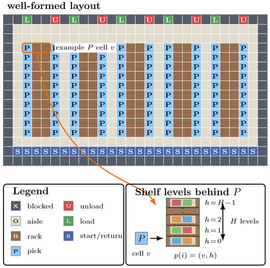
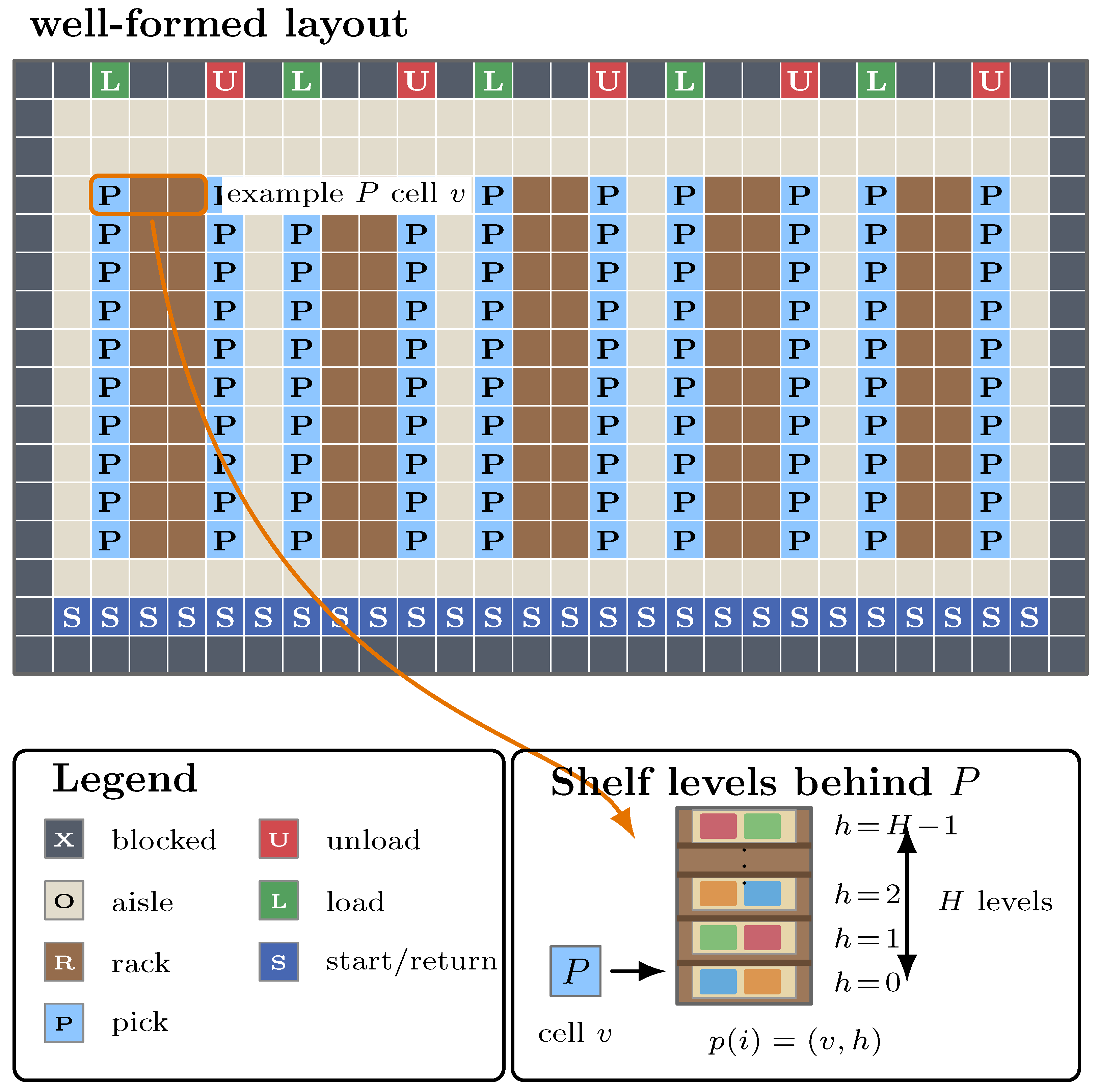
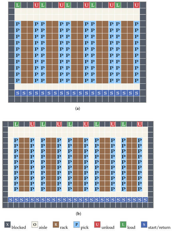
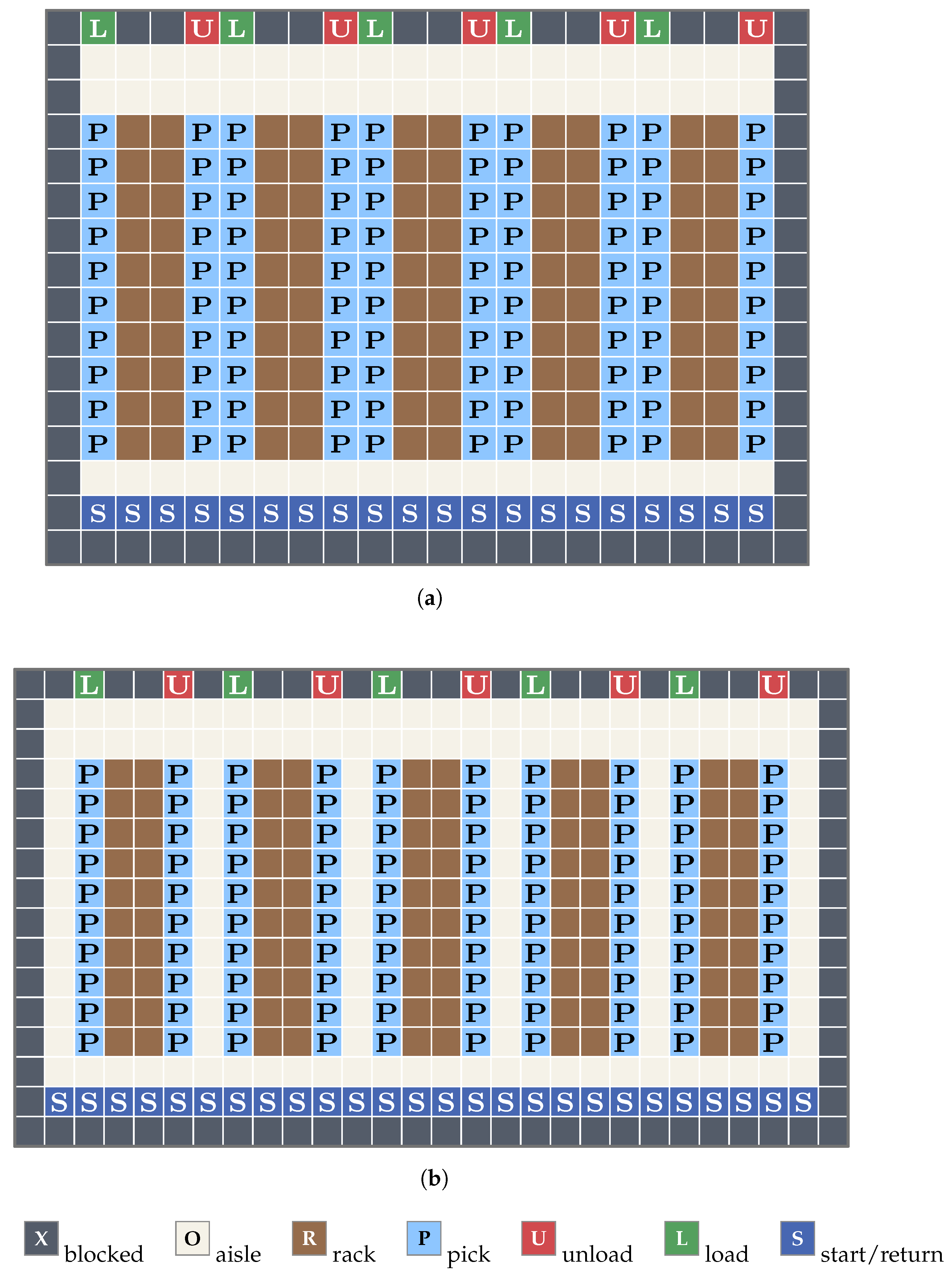
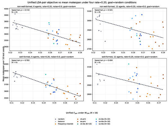
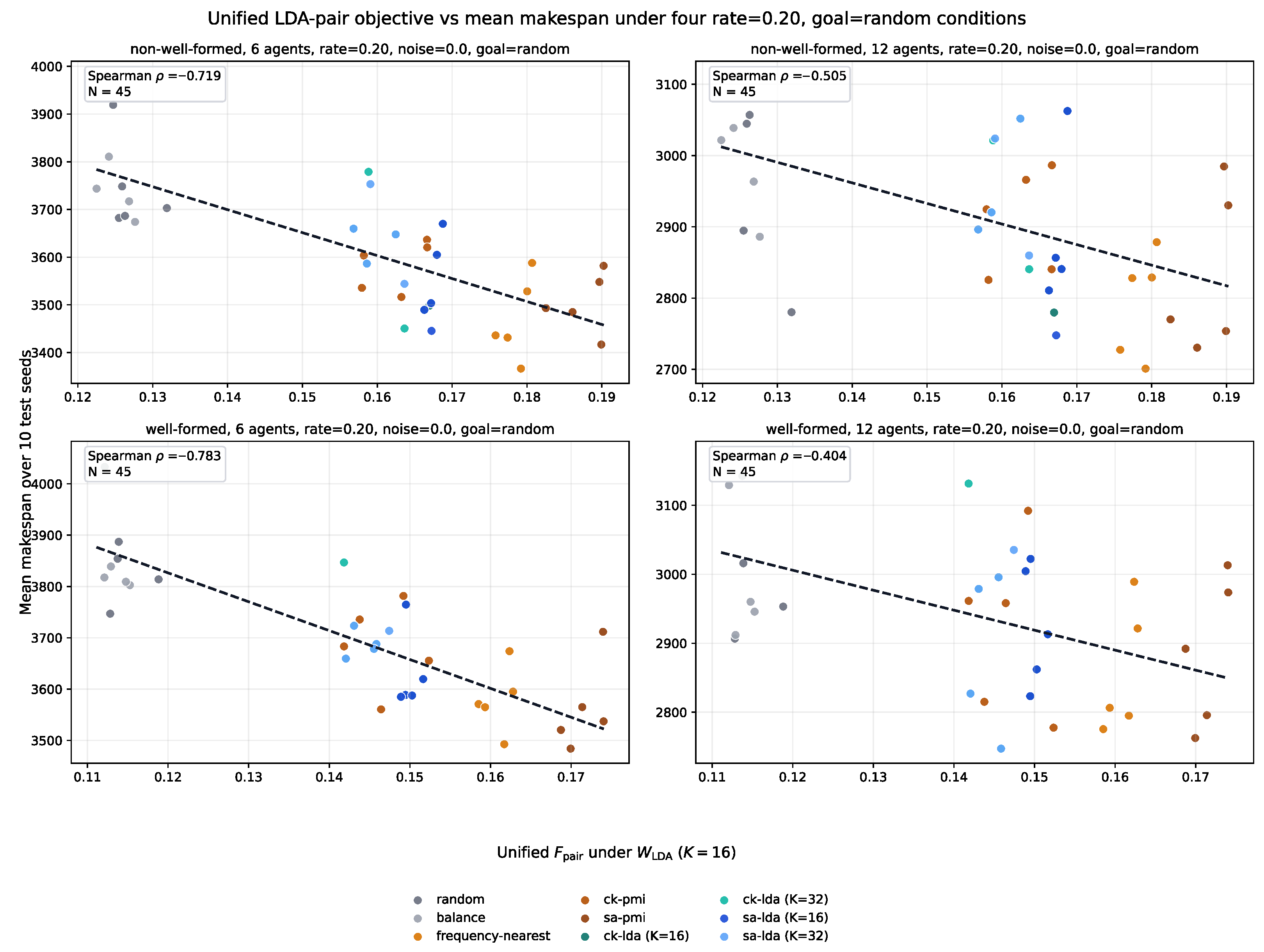

Disclaimer/Publisher’s Note: The statements, opinions and data contained in all publications are solely those of the individual author(s) and contributor(s) and not of MDPI and/or the editor(s). MDPI and/or the editor(s) disclaim responsibility for any injury to people or property resulting from any ideas, methods, instructions or products referred to in the content. |
© 2026 by the authors. Licensee MDPI, Basel, Switzerland. This article is an open access article distributed under the terms and conditions of the Creative Commons Attribution (CC BY) license.