


Abstract
This study benchmarks three ROS 2 Navigation2 local controllers—Dynamic Window Approach Based (DWB), Regulated Pure Pursuit (RPP), and Model Predictive Path Integral (MPPI)—under three complementary operational stressors in simulation: (i) a structured corridor with a transient dynamic obstacle, (ii) a sloped environment where terrain inclination biases a planar 2D LiDAR costmap through spurious occupancy projections, and (iii) a narrow corridor that amplifies inflation effects. A reproducible rosbag2-based protocol records five key performance indicators per trial: time-to-goal, lateral tracking RMSE, stopped time, heading oscillations, and control effort. With 15 independent repetitions per cell (scene × controller × direction), the design yields 270 trials. The results expose complementary value profiles: RPP minimizes mission time, DWB produces the fewest heading oscillations through critic-based shaping, and MPPI achieves the lowest control effort via smooth trajectory generation. In the sloped scene, the tracking RMSE differences compress across all controllers—a signature of a perception-limited regime in which costmap bias overshadows controller logic. These findings translate into an actionable controller-selection guide and a reproducible baseline for quantifying gains from upstream perception and cost-representation improvements. In concrete terms, we contribute (i) a controlled benchmark with fixed planning, localization, and costmaps, (ii) full configuration disclosure (controller parameters, costmap settings, and software versions with package pinning), and (iii) a scene-specific costmap distortion index that links slope-induced local cost bias to measurable performance shifts, underpinning a decision matrix for controller selection in semi-structured environments.
1. Introduction
Local trajectory planning within the ROS 2 ecosystem, implemented through the Navigation2 (Nav2) software stack, has become a de facto standard for autonomous mobile robot deployment in both academic and industrial settings. Field experience, however, repeatedly shows that end-to-end navigation performance is often limited not by the sophistication of the controller itself but by the fidelity of the perception-to-costmap pipeline. The issue is especially acute in semi-structured and subterranean domains, where irregular terrain and degraded sensing conditions inject systematic bias into obstacle evidence, inflate conservative maneuver margins, and shrink the effective navigable free space [1,2,3,4,5,6]. A well-documented failure mode arises when planar two-dimensional Light Detection and Ranging (2D LiDAR) sensors operate over non-planar surfaces: vehicle pitch and roll, combined with ground-level height discontinuities, violate the planar scanning assumption. As a result, sensor returns are projected into spuriously occupied grid cells, generating artificial inflation-induced bottlenecks in the local costmap [7].
Recent systems-oriented work in underground mining confirms this view, showing that enriching the perception-to-cost pipeline with semantic risk encoding can reshape navigation trade-off surfaces in non-trivial ways [8]. In deliberate contrast, the present study retains a purely geometric perception pipeline to establish a rigorous controller-level baseline before any semantic augmentation is introduced.
The Nav2 architecture is well suited for controlled comparisons thanks to its modular plugin design, which allows swapping the local controller while keeping global planning, localization, costmap fusion, and perception preprocessing unchanged [9,10,11]. Building on recent benchmarking work [12], we compare three representative local controllers that span distinct control-theoretic families: (i) Dynamic Window Approach as implemented by Nav2’s DWB controller (DWB, velocity sampling with weighted multi-objective critics) [13,14], (ii) Regulated Pure Pursuit (RPP, geometric path-following augmented with adaptive regulation and collision checking) [15,16], and (iii) Model Predictive Path Integral (MPPI, stochastic optimal control with soft-minimum trajectory aggregation) [17,18,19,20].
We evaluate these controllers under three complementary stressors: (i) a structured corridor with a transient dynamic obstacle, (ii) a sloped semi-structured environment that biases a 2D LiDAR-derived costmap, and (iii) a narrow corridor with tight geometric margins. Each controller runs in both travel directions ( and ) with repetitions per cell, yielding 270 trials. All trials are logged with rosbag2 for traceability [21,22,23], and five operational metrics are computed: time-to-goal, plan-tracking RMSE, stopped time, heading oscillations, and a control-effort proxy [8]. Robust summaries (medians and IQR) together with rank-based inferential comparisons support decision-making beyond individual runs.
This study addresses two questions: (Q1) which controller advantages persist when the dominant limitation is upstream (perception-to-cost fidelity) rather than controller optimization? and (Q2) how do mission-relevant trade-offs among time, tracking, angular stability, and effort re-balance across stressor regimes? Our contributions are: (1) a reproducible rosbag2-driven acquisition and analysis protocol; (2) a three-scene benchmark that disentangles transient obstacle interactions, systematic costmap bias, and tight-margin navigation; and (3) a decision-oriented synthesis that maps controllers to stable value profiles across regimes.
Scope is intentionally limited to local control on a differential-drive platform with fixed 2D costmaps. We do not propose new critics, layers, or perception modules; rather, we characterize comparative behavior under controlled conditions to establish a geometry-only baseline for future cost/perception enrichments.
2. Related Work and Theoretical Background
2.1. Navigation2 Architecture and Reproducible Evaluation
In ROS 2 Nav2, a global planner produces a polyline in the map frame; the global and local costmaps fuse static, obstacle, and inflation layers; and the controller server issues commands for the base [9,10]. For reproducible benchmarking, the key requirements are: fix the perception and localization parameters, swap only the controller plugin, log each trial with rosbag2, and report metrics that cover temporal efficiency, path tracking, angular stability, and actuation cost [11,21]. Recent comparative studies further recommend holding the costmap configuration constant across runs because changes in resolution, inflation radius, or update rates can dominate local decision-making and confound controller attributions [12,24,25]. In multi-robot settings with formation and obstacle constraints, the constraint formulation itself strongly shapes feasible motions and resulting trajectories [26]. When extending single-robot controller comparisons to such settings, constraint models should therefore be aligned to prevent confounded interpretations.
Beyond controller-only swaps, repeatability in navigation is also shaped by (i) simulation determinism, (ii) consistent random seeds for obstacle motion when used, (iii) fixed update frequencies across Nav2 servers, and (iv) stable middleware timing assumptions (e.g., simulated time) to avoid subtle drift in controller invocation and costmap refresh. In ROS 2, end-to-end reproducibility is facilitated by standardized logging pipelines and data-centric evaluation workflows, where a single rosbag2 dataset can be replayed to verify metric computation and to support ablation studies on analysis choices [21,22]. This mirrors broader benchmarking efforts in mobile robotics that advocate standardized scenario batches and progressive difficulty, especially when dynamic obstacles are involved [27,28].
Complementarily, several open platforms have emerged to lower the barrier for controller benchmarking and scenario management in ROS 2-centric workflows. Web-based suites and benchmark platforms provide consistent simulation harnesses and make it easier to compare classical planners against learning-based approaches under shared conditions [29,30,31]. Within this landscape, Nav2’s plugin architecture remains attractive for controlled local-controller comparisons precisely because it allows holding global planning, localization, and costmap pipelines fixed while swapping only the controller and its parameters [9,11].
2.2. Costmaps, Layers, and Controller–Perception Coupling
Local planners in Nav2 are only as reliable as the local costmap signals they consume. Even when global planning is stable, short-horizon decisions can be dominated by layer semantics (static, obstacle, and inflation), update timing, and the projection of sensor artifacts into occupancy. Recent work shows that real-time costmap update strategies—for instance, in agricultural settings—materially affect local planning by reducing stale obstacle evidence and improving responsiveness [32]. The community is also moving toward richer cost representations beyond binary occupancy, including object- or affordance-aware costmaps that enable proactive collision avoidance [33].
This coupling matters most when the environment violates planar assumptions. Under slopes or uneven ground, a corridor that is geometrically safe may become artificially narrow once sensor returns are projected into 2D occupancy and inflated. In such a regime, controller differences reflect not only optimization logic but also how each algorithm reacts to biased cost gradients—whether by braking, steering aside, or oscillating. This observation motivates testing controllers under both favorable (costmap faithful to geometry) and adverse (costmap biased by perception limits) conditions [9,11].
Semantic Risk-Aware Cost Encoding and Effort-Aware Trade-Offs
Beyond purely geometric occupancy, recent mining-oriented systems work has shown that injecting semantic risk into the perception-to-cost pipeline can systematically reshape navigation trade-offs while preserving compatibility with ROS planner interfaces [8]. In particular, semantic priority encoding and risk-adaptive inflation can increase minimum clearance to high-priority obstacles with a modest increase in kinematic effort, reinforcing that upstream perception and cost representations are first-order levers for end-to-end behavior [8]. In contrast, the present study keeps the perception stack unchanged and analyzes the complementary regime, where costmap distortion is induced by geometric sensing limits (2D LiDAR on slopes), isolating controller behavior under perception-limited costs.
Table 1 summarizes representative strands that frame this work: controller families, upstream cost/perception factors shaping the local decision space, and benchmarking practices enabling like-for-like comparisons.
Table 1.
Compact taxonomy of representative works relevant to Nav2 local navigation (controllers, costmaps, and benchmarking).
2.3. Dynamic Window Approach
The Dynamic Window Approach discretizes admissible velocities under kinematic limits, rolls out short arcs, and evaluates them with a weighted sum of costs reflecting goal progress, plan adherence, and obstacle clearance [13]. In Nav2, DWB exposes configurable critics including PathDist, GoalDist, GoalAlign, BaseObstacle, and oscillation/twirling suppression, providing explicit levers to penalize unnecessary heading reversals and to stay near the global plan [14]. Recent variants accelerate sampling and pruning or refine obstacle handling to cut evaluation time while preserving local safety [35,36]. In practice, the short-horizon rollout and critic stacking of DWB bias solutions toward predictable heading behavior, typically producing low counts of sign changes in when the costmap is stable.
More broadly, DWB-style velocity sampling sits within a large family of local planning methods that trade compute for robustness by evaluating many feasible commands against cost functions. Comparative studies that include classic sampling-based planners alongside learning-based policies typically find that classical approaches remain competitive when sensing and mapping are reliable but may degrade sharply when the perceived free space is biased or delayed [29,37]. This motivates the inclusion of metrics that diagnose not only speed or tracking but also stop-and-go behavior and oscillatory corrections under inflated costs.
2.4. Regulated Pure Pursuit
Pure Pursuit aligns the robot toward a lookahead point sliding along the global path; Regulated Pure Pursuit extends this geometry with linear-velocity regulation based on curvature and costmap values, plus forward collision checks [15,16]. The regulation prevents abrupt braking in tight passages and increases stability in bends, often sustaining competitive speeds on straight, low-cost segments. In practice, behavior depends on the lookahead policy and on the gains for curvature and cost regulation. In corridors with few conflicts, the geometry-first design of RPP often translates into a short time-to-goal; in narrow or cost-inflated areas, it reduces speed smoothly rather than stopping.
The recent path-tracking literature continues to refine pure-pursuit-style controllers via multi-objective tuning and robustness improvements under real sensing constraints, reinforcing that geometry-driven tracking can be strong when the global plan is trustworthy and costs are well-calibrated [38]. However, in perceptually degraded settings, the effectiveness of RPP can hinge on whether the cost regulation reacts too aggressively to spurious occupancy, producing conservative slowdowns that dominate time-to-goal without necessarily improving tracking error.
2.5. Model Predictive Path Integral
MPPI samples control sequences, simulate their state rollouts with a kinematic (or dynamic) model, and aggregate costs using a soft-min weighting. Specifically, each sampled trajectory with cost receives weight , and the commanded control is the weighted average of the samples. The scalar is the “temperature”: small makes the soft-min sharp (a few low-cost rollouts dominate, yielding reactive, possibly chattering behavior), whereas large flattens the weights (many rollouts contribute, yielding smoother but more conservative commands) [17,18,19]. Penalizing input magnitudes with a quadratic term further biases solutions toward low-amplitude commands, which correlates with reduced actuation effort and fewer full stops. The Nav2 implementation exposes batch size, horizon length, exploration standard deviations, and temperature , letting practitioners trade responsiveness against smoothness and compute [39]. MPPI has also been adapted to robustness-oriented domains beyond ground navigation, highlighting its generality as a sampling-based stochastic optimal control method [20].
In recent years, MPPI has also been extended in directions that are directly relevant to practical navigation: leveraging fast parallel simulation, biasing sampling with auxiliary controllers, and improving performance under constrained compute [40,41]. Importantly for non-planar or semi-structured scenes, MPPI has been demonstrated with terrain-aware representations (e.g., 2.5D/elevation maps), indicating that controller smoothness benefits may persist when the cost representation captures slopes more faithfully than a 2D occupancy projection [42]. This reinforces the key question in this paper: how much of the MPPI value profile survives when the dominant bottleneck is costmap bias rather than controller optimization.
2.6. Perception Limits with 2D LiDAR
In underground or semi-structured environments, sensing artifacts such as dust and adverse conditions can bias range returns and corrupt the obstacle evidence feeding 2D costmaps, amplifying conservative inflation and recovery behaviors [1,3,4,43,44].
On non-planar terrain, a planar 2D LiDAR combined with scan-to-grid rendering can inject systematic bias into occupancy: partial ground returns and height discontinuities are rendered as occupied cells and subsequently inflated, producing spurious bottlenecks and apparent corridor narrowing [34,45]. These artifacts can dominate the effective local decision space, amplifying trade-offs in time, angular stability, and actuation effort, and motivating evaluation under perception-limited cost representations [9,11].
Terrain-aware navigation pipelines increasingly incorporate 2.5D or semantic terrain representations to reduce false occupancy and to reason about traversability explicitly [46,47]. By contrast, when a planar 2D LiDAR feeds a 2D costmap, slopes act as a systematic bias injected into the controller’s cost function. Under that lens, comparing controllers in sloped scenes partly measures robustness to biased costs rather than pure tracking capability.
2.7. Metrics and Interpretation
The metrics adopted here reflect widely used operational KPIs. Time-to-goal captures temporal efficiency and is sensitive to regulation and conflict resolution near inflated costs. Lateral tracking error is computed as the orthogonal point-to-segment distance from the executed trajectory to the global plan and summarized as RMSE; its interpretation must account for the plan selection window and local replanning behavior. Stopped time quantifies operational idling via a near-zero velocity threshold and is useful for detecting freeze-like behaviors. Heading oscillations count sign changes in , serving as a proxy for zig-zag corrections and short-horizon indecision [48,49]. Control effort, defined as , serves as a kinematic-effort proxy [8].
Recent benchmarking protocols often add success-rate and collision-centric safety indicators together with path-length and smoothness families, particularly in settings involving humans or dynamic obstacles [28,50]. Here, we opt for a compact metric set aligned with mission execution and controller behavior diagnosis (speed, tracking, stopping, oscillations, and effort), while preserving rosbag2 traceability for future extensions with additional safety or comfort metrics [21,22].
2.8. Our Positioning
While comparative reports exist, few studies isolate the controller as the sole changing variable while holding global planning, localization, costmaps, and sensor parameters fixed across scenes. Even fewer explicitly separate a transient obstacle stressor from a slope-induced perceptual stressor within the same benchmark. By adopting a rosbag2-driven, reproducible protocol [21,22], this work provides a basis to map each controller to a robust value profile across environments—RPP for speed, DWB for angular stability, MPPI for smoothness/effort—and to motivate future work targeting the dominant error source under slopes: perception and costmap quality.
In particular, recent directions in navigation research stress the importance of improving fidelity and semantics in cost representations (e.g., real-time local updates and object-aware costmaps) to unlock controller performance in perceptually challenging settings [32,33]. Our benchmark complements these efforts by showing what can (and cannot) be achieved when the costmap remains 2D and perception-limited, thereby clarifying whether gains should be pursued primarily at the controller level or upstream in sensing and mapping.
3. Methodology
3.1. Experimental Setup and Control Stack
Experiments were conducted on a simulated differential-drive platform (Clearpath Husky A200) running Ubuntu 22.04, ROS 2 Humble, Nav2, and Gazebo Ignition Fortress bridged via ros_gz [9,51]. Global planning, localization, and costmaps were held constant across all runs so as to isolate the local controller’s effect. Localization relied on AMCL with standard Nav2 integration [52]. Both global and local costmaps combined static, obstacle, and inflation layers at fixed resolution, inflation radius, update/publish rates, and rectangular footprint. Only the local controller plugin and its internal parameters were varied among DWB, RPP, and MPPI [10,11,14,15,19,39]. Obstacle information came from a simulated planar 2D LiDAR feeding the local costmap obstacle layer through the Nav2 laser scan integration.
3.2. Scenarios and Trial Protocol
Three complementary scenes were used. Scene 1 is a structured corridor with a single transient dynamic obstacle on the outbound leg; depending on costmap clearing behavior and update timing, inflated costs may persist briefly after the obstacle leaves the sensing frustum. Scene 2 is a semi-structured environment with slopes and uneven surfaces; a planar 2D LiDAR can render elevation changes as occupied cells in 2D grids, creating spurious bottlenecks. Scene 3 is a narrow corridor that enforces tight geometric margins, amplifying inflation and short-horizon conflict resolution. Scenes and goal placement are illustrated in Figure 1.
Figure 1.
Evaluation scenes and goals. (a) Scene 1: structured corridor with a transient dynamic obstacle on . (b) Scene 2: semi-structured slopes; S and G positioned to enforce an uphill segment on . (c) Scene 3: narrow corridor enforcing tight geometric margins. The costmap is overlaid.
For each scene, controller, and direction (S → G and G → S), 15 independent repetitions were executed under identical arrival conditions and system parameters, yielding a total of 270 trials (3 scenes × 3 controllers × 2 directions × 15 repetitions).
3.3. Data Acquisition with Rosbag2
Each trial was logged using rosbag2 in SQLite3 format (.db3) for traceability and offline analysis via Python 3.10 [21,22]. Logging was triggered programmatically from the task scripts that also published goal coordinates for outbound and return runs. Table 2 lists the recorded topics used in the metrics pipeline, including the simulated clock to reconstruct a coherent chronology with use_sim_time enabled. The experimental methodology is summarized in Figure 2.
Table 2.
Recorded data used for metrics (rosbag2/SQLite3).
Figure 2.
Experimental methodology flowchart.
Bags were named {controller}_{forward|return}_{trial}_{timestamp}.db3, one file per attempt. Logging depth and I/O parameters were chosen to prevent drops; when necessary, QoS overrides were used to match publisher/subscriber reliability for high-rate sensors [9,11,21]. Bags were associated with each scene via the corresponding launch configuration and output directory used during data collection; summaries and per-trial CSVs are stored per-scene to preserve traceability.
3.4. Preprocessing, Synchronization, and Plan Selection
Time origin was defined as the first timestamp of /goal_pose. If /goal_pose was missing, the first odometry message was used. All signals were cropped to , where was the first arrival instant when the AMCL position entered a radius r around the goal and remained within it for at least h (yaw unconstrained).
Plan selection followed a robust rule: among the plans published in the window with s, the polyline with the largest geometric length was chosen from /plan and /received_global_plan. This strategy mitigates bias from short transient plans and provides a consistent reference. Lateral RMSE is computed with respect to this selected reference plan to ensure like-for-like comparability across controllers, even when replanning occurs during a trial.
Pose source priority was AMCL. If AMCL was unavailable or inconsistent early on, odometry was aligned to the map frame by estimating a rigid 2D transform—one planar rotation plus a translation—from early correspondences to the selected plan, and then re-expressing the odometry trajectory in map coordinates. Simulated time was used throughout; recording /clock with use_sim_time enabled avoided cross-topic timing inconsistencies [53].
For derived quantities, finite differences with protection against very small were used; non-monotonic or duplicated timestamps were ignored and replaced by a minimum positive sampling interval.
3.5. Metrics Definition
We report five metrics that jointly capture task completion, tracking accuracy, and dynamic feasibility. Let be the time when the goal is issued and let be the robot position. The global plan is represented as a polyline and the commanded twist as .
- Time-to-goal.
Let the goal position be and define the arrival time as the first t such that the robot remains within a radius for a dwell time :
The time-to-goal is then .
- Lateral tracking error (RMSE).
For each sample, let be the Euclidean distance from to the closest point on the global plan polyline. The lateral RMSE is
- Stopped time.
Define and an inactivity threshold . The stopped time accumulated during the trial is
For completeness, the stopped-time ratio is .
- Heading oscillations.
Let and define the sign function . The oscillation count is the number of non-zero sign changes:
- Control effort.
We approximate actuation effort by the command energy (squared-command integral) over the trial,
which penalizes sustained high-magnitude translational and rotational commands. In the released dataset, this corresponds to cmd_lin_L2+cmd_ang_L2. It is important to note that is a post hoc evaluation KPI, not an optimization objective within any controller’s internal cost function. Each algorithm pursues its own formulation during execution: DWB selects trajectories by minimizing a weighted critic sum that balances progress, clearance, and alignment; RPP tracks the global path through a regulated pursuit law with curvature and collision constraints; and MPPI aggregates sampled roll-outs via soft-minimum weighting over a user-defined running cost. The metric is computed after each trial from the recorded /cmd_vel stream, providing a uniform basis to compare the actuation intensity that each strategy produces under identical mission conditions.
We summarize each metric using the median and the interquartile range (IQR), defined as
where and denote the 25th and 75th percentiles, respectively.
3.6. Costmap Distortion Metric for Scene 2
To quantify slope-induced bias in the local cost representation, we define a per-trial costmap distortion index measuring the fraction of high-cost cells within a fixed-radius neighborhood around the robot footprint. The metric is computed from the recorded local costmap and robot pose, with no modifications to the Nav2 stack.
Let denote the local costmap at time t (Nav2 nav_msgs/msg/OccupancyGrid published on /local_costmap/costmap), and let be the robot position in the costmap frame. For a fixed evaluation radius m around the robot footprint, define the set of grid cells inside that disk as . Each cell has an occupancy cost , where denotes unknown and larger values indicate higher collision risk (inflation/lethal).
We define the instantaneous high-cost fraction around the robot as
where and . The per-trial distortion score is the mean over the navigation interval,
We also monitored the unknown-cell fraction inside ; it was consistently negligible in our rolling-window local costmap during motion.
Figure 3 provides qualitative evidence for this phenomenon, showing the slope geometry, the raw planar scan projection, the resulting inflated costmap, and the footprint-clearing effect in Scene 2.
Figure 3.
Scene 2 qualitative evidence of slope-induced planar-scan artifacts and their effect on the rolling local costmap. (a) Gazebo side-view of the sloped segment; the yellow polyline traces the local terrain profile that violates the planar 2D LiDAR assumption. (b) RViz overlay of raw planar LaserScan endpoints (red) on the 2D map, showing off-plane returns projected into the corridor. (c) Resulting rolling local costmap with inflation enabled: inflated high-cost bands (cyan/magenta) narrow the feasible corridor. (d) Footprint clearing in the rolling costmap: cells are repeatedly cleared in the immediate footprint vicinity while nearby inflated artifacts persist along the passage.
3.7. Per-Trial Computation Pipeline
The analysis pipeline applied the same sequence to each .db3:
- Determine from /goal_pose; if absent, from the first odometry sample. Crop all signals to , where is the arrival time.
- Select the global plan using the robust window rule with s and longest-length criterion across /plan and /received_global_plan.
- Choose the pose source: AMCL is preferred; otherwise, align the odometry to the map by fitting a rigid 2D transform (rotation + translation) and rewrite the odometry trajectory in map coordinates.
- Compute the five metrics over using finite-difference derivatives, thresholding for stopped time, and sign-change counting for oscillations.
- Write one CSV row per attempt containing metrics and metadata (controller, direction, trial index, and parameters).
3.8. Aggregation and Visualization
For each scene, controller, and direction, medians across 15 trials were reported for the five metrics, together with interquartile ranges (IQRs) as a dispersion statistic. Totals were computed as outbound plus return for time-to-goal, stopped time, oscillations, and control effort. For lateral RMSE, per-direction medians were reported; for compact comparison across controllers, their sum was included consistently with the analysis dataset. We report the sum of per-direction medians as a compact composite indicator (not as a distributional statistic).
3.9. QoS and Loss Mitigation
Publisher–subscriber QoS compatibility influences both recording and replay. Reliability and durability policies were configured to match the expected producers and consumers; for high-rate or lossy sensors such as 2D LiDAR, best-effort publishers may be preferable, while map and costmap channels were kept reliable [9,11,21]. Subscriber queue depths were set to a sufficiently high value of 50 to avoid drops during transient bursts; simulated time was enforced during both recording and offline processing [53].
3.10. Default Parameters and Reproducibility
Unless stated otherwise, the following defaults were used: positional radius m, hold time s, yaw threshold with hold s when required, stopped-time threshold m/s, and plan-selection window s. Orientation thresholds (, ) are defined in the pipeline for future extensions but were not applied in this study (position-only arrival). The pipeline is deterministic given the rosbag2 logs and the parameter settings reported here, and it is scriptable end-to-end: rosbag2 logging, plan selection, metric computation, and figure generation [21,22].
- Software versions.
All experiments used ROS 2 Humble on Ubuntu 22.04 (Jammy) with Nav2 installed from the ROS apt repository at version 1.1.20 (Debian build stamps 20251228). The Gazebo integration used ros-humble-ros-gz version 0.244.20 (build stamps 20251228), running on Gazebo Sim 6.17.0. Since these packages were installed from the official ROS apt repository as pre-built Debian binaries, upstream Git commit hashes are embedded in the Debian changelog and can be retrieved via apt-get changelog ros-humble-navigation2; the corresponding source tarball (and thus the exact commit) is also pinned in the repository snapshot. The full dpkg -l listing for all ROS packages used in this study is archived in the data repository alongside the rosbag2 logs to ensure bit-exact reproducibility.
- Controller and costmap configurations.
To maximize comparability, we start from the default controller parameterizations maintained by Nav2 and then adjust only what is required to (i) enforce identical kinematic limits and (ii) avoid obviously unfair advantages (e.g., mismatched horizons or sampling budgets). Table 3 consolidates the exact settings used for DWB, RPP and MPPI. In addition, Table 4 reports the fixed local/global costmap configuration (resolution, inflation, update/publish rates, window size and footprint), which is identical across all runs.
Table 3.
Consolidated controller configuration used across runs (only the local-controller plugin and its internal parameters change; all other Nav2 components and costmaps remain fixed).
Table 4.
Fixed costmap configuration (identical across controllers and runs). Values are taken from the Nav2 YAML used in all experiments.
4. Results
This section reports the navigation performance of three Nav2 local controllers (DWB, RPP, and MPPI) across three scenes designed to stress complementary failure modes: (i) a structured corridor with a transient dynamic obstacle, (ii) a sloped scene where terrain distorts the 2D LiDAR-derived local costmap, and (iii) a narrow corridor that amplifies inflation. The design is fully crossed: each controller was evaluated in both directions ( and ) with independent repetitions, yielding 270 successful trials. Arrival was assessed using a position-only condition (yaw unconstrained); all trials met the criterion and none were excluded.
Results are presented in two layers. First, robust descriptive statistics (median and interquartile range, IQR) per controller and direction characterize central tendency and dispersion under the non-Gaussian behavior typical of navigation timing and interaction events. Second, inferential statistics assess whether controller differences are statistically supported within each scene, complemented by effect sizes and multiple-comparison control.
Five operational metrics are analyzed, aligned with the methodology: time-to-goal , lateral tracking error relative to the selected global plan (RMSE), stopped time , heading oscillations (sign changes of ), and a control-effort proxy defined as the integral of squared commanded velocities. Metrics were computed per trial from rosbag2 logs using a deterministic pipeline; the per-trial dataset is the source of truth for all tables and figures. For traceability, results are organized by scene and direction.
4.1. Descriptive Statistics (Baseline)
As a baseline, each metric is summarized with robust descriptive statistics (median and IQR) over the repetitions in every controller–direction cell. This choice is motivated by the skewness and heavy tails commonly observed in navigation outcomes (e.g., stop episodes and interaction events), where mean–variance summaries can be misleading. Unless otherwise stated, tables report medians separately for the outbound () and return () legs.
For control effort, we report the per-trial proxy as implemented in the dataset via the sum of the linear and angular squared-command integrals ().
4.1.1. Scene 1: Structured Corridor — Descriptive Summary
In Scene 1 (Table 5), the strongest separation appears in time-to-goal: RPP shows the lowest medians on both legs, while MPPI is consistently slower. Tracking behavior reveals a complementary profile: DWB attains the lowest return-leg RMSE, whereas RPP exhibits the largest RMSE dispersion on the return leg, consistent with more variable convergence after interaction events. Stop behavior is markedly asymmetric for DWB, with a much larger return-leg stopped-time median and IQR, indicating more frequent stop-and-go episodes. MPPI maintains the lowest effort profile across both legs, indicating smoother low-amplitude command sequences despite longer traversal times.
Table 5.
Scene 1 (structured corridor): descriptive statistics by controller and direction (median [IQR]).
4.1.2. Scene 2: Semi-Structured Slopes — Descriptive Summary
Scene 2 (Table 6) compresses the tracking differences relative to Scene 1, consistent with a perceptual bottleneck: slope-induced false occupancy constrains the feasible corridor in the 2D costmap. RPP remains fastest in median time-to-goal, with DWB close on both legs. MPPI again yields the lowest effort, while exhibiting noticeably higher oscillation counts; descriptively, this indicates frequent small heading corrections under an unstable free-space estimate, yet with low command energy. Stopped-time medians are on the order of ∼1 s or below, suggesting that delays stem more from cautious progression and corrective steering than from prolonged halts. To quantify the local cost bias directly, Table 7 reports the costmap distortion index (and its unknown/high-cost components), computed from the recorded local costmap around the robot footprint.
Table 6.
Scene 2 (semi-structured slopes): descriptive statistics by controller and direction (median [IQR]).
Table 7.
Costmap distortion summary for Scene 2 (median [IQR] across trials per direction). is the mean high-cost fraction within a disk of radius m around the robot footprint (Section 3.6).
4.1.3. Sensitivity to Costmap Distortion (Scene 2)
Because Scene 2 is dominated by a perception-to-costmap bias that varies across trials, we complement the factorial comparisons with a targeted sensitivity analysis on the costmap distortion index . Trials are stratified into low and high distortion groups using the global median over Scene 2 (both directions pooled). Table 8 reports robust within-stratum medians of completion time, the control-effort proxy, and oscillation counts. In this regime, MPPI shows the largest degradation under high distortion (increased completion time and oscillations), DWB exhibits the most stable medians across strata, and RPP remains competitive in time but trends toward higher oscillation counts as distortion increases. The stratified results thus link an environmental nuisance variable () to the metrics that become most discriminative in Scene 2, and help explain controller behavior under perception-biased local costs.
Table 8.
Scene 2 sensitivity analysis to the local costmap distortion index. Trials are split into low and high distortion by the global median over all Scene 2 trials (both directions pooled). Each cell reports the within-bin median of the distortion index and performance metrics: completion time T (s), control-effort proxy (squared-command integral), and oscillations count O. The number of trials n varies by controller and bin because the split is performed globally.
4.1.4. Scene 3: Narrow Corridor—Descriptive Summary
In Scene 3 (Table 9), tight margins amplify short-horizon corrections, making oscillations and effort the most discriminative indicators. RPP preserves the time advantage on both legs but exhibits higher tracking RMSE than DWB and MPPI, indicating larger lateral deviations under corridor constraints. MPPI continues to minimize (and slightly reduces stopped time), yet accumulates the largest oscillation counts, consistent with frequent micro-corrections while maintaining low-energy actuation. DWB shows the lowest oscillation levels among the three controllers, with intermediate time-to-goal and effort comparable to RPP (and consistently higher than MPPI).
Table 9.
Scene 3 (narrow corridor): descriptive statistics by controller and direction (median [IQR]).
To complement Table 5, Table 6, Table 7, Table 8 and Table 9, Figure 4 visualizes the full per-trial distributions ( per controller–direction cell) of time-to-goal and plan-tracking RMSE across the three scenes. The boxplots make dispersion and direction-dependent asymmetries explicit, highlighting the RPP throughput advantage and the RMSE compression in the perception-limited sloped environment (Scene 2).
Figure 4.
Per-trial distributions of time-to-goal and plan-tracking RMSE across scenes, controllers, and directions ( per controller–direction cell). Boxes show median and IQR; whiskers extend to 1.5 IQR; outliers are omitted for readability. Direction is indicated by hatch pattern.
Figure 5 reports the corresponding distributional view for oscillations and the effort proxy . This visualization supports the interpretation that DWB stabilizes heading decisions (lower oscillation counts), while MPPI consistently reduces actuation intensity (lower ), even when oscillation counts increase under constrained or perception-distorted free space.
Figure 5.
Per-trial distributions of heading oscillations and control-effort proxy across scenes, controllers, and directions ( per controller–direction cell). Boxes show median and IQR; whiskers extend to 1.5 IQR; outliers are omitted for readability. Direction is indicated by hatch pattern.
4.2. Inferential Statistics (Controller and Direction Effects)
Beyond the descriptive baseline in Table 5, Table 6, Table 7, Table 8 and Table 9, we test whether the observed performance differences are statistically supported under the fully crossed design (Controller × Direction) within each scene. Because navigation metrics often deviate from Gaussian assumptions (skewness, heavy tails, and discrete interaction counts), we adopt a rank-based factorial approach. For each metric and scene, the Scheirer–Ray–Hare test assesses the main effects of the controller and direction, as well as their interaction. We report p-values alongside a rank-based effect size (computed as for each factor).
When the controller main effect is significant, we follow with post hoc comparisons between controllers (DWB, MPPI, RPP) using two-sided Mann–Whitney U tests. If the Controller × Direction interaction is significant, post hoc tests are reported within each direction; otherwise, comparisons are reported on pooled data across directions. Within each family of three pairwise contrasts, p-values are corrected using Holm’s method. The practical magnitude is summarized with Cliff’s and the median difference (first minus second).
4.2.1. Scene 1: Structured Corridor—Factorial and Post-Hoc Analysis
Table 10 confirms statistically supported controller differences for all five metrics in Scene 1. Direction-dependent effects are consistent with the transient disturbance on and with traversal asymmetries when the corridor is navigated in reverse under the same fixed costmap and controller settings. Accordingly, post hoc comparisons for those metrics are reported within each direction, while time-to-goal and control effort are compared on pooled data (no interaction).
Table 10.
Scene 1: rank-based factorial tests for controller and direction effects (Scheirer–Ray–Hare). (Factors: controller, direction, and interaction; effect size reported as ).
Post hoc outcomes in Table 11 operationalize the Scene 1 trade-offs. On pooled data, RPP is significantly faster than both DWB and MPPI in time-to-goal, and MPPI is also significantly slower than DWB. For control effort, MPPI is significantly lower than both DWB and RPP, reinforcing its low-effort profile. For interaction-driven metrics, direction dependence emerges: on the return leg, tracking RMSE separates all controllers (DWB < MPPI < RPP), while on the outbound leg RMSE separates MPPI from RPP. The return-leg stopped time is also fully separated (DWB > RPP > MPPI), and return-leg oscillations are lower for DWB than for both MPPI and RPP.
Table 11.
Scene 1: significant post hoc controller differences (two-sided Mann–Whitney U with Holm correction). (Pairwise Wilcoxon rank-sum with Holm correction; Cliffs effect size.)
4.2.2. Scene 2: Semi-Structured Slopes — Controller and Direction Effects
Scene 2 (Table 6) is dominated by a perceptual stressor: slope-induced projections into a planar 2D costmap intermittently constrain free space and can amplify small steering corrections. The rank-based factorial results in Table 12 show statistically supported controller effects for all five metrics but with smaller effect sizes than in Scene 1 for RMSE and stopped time. Direction effects are significant for time-to-goal and control effort, indicating systematic outbound/return asymmetry in traversal dynamics. A controller×direction interaction is detected for RMSE, motivating direction-stratified post hoc comparisons for tracking behavior.
Table 12.
Scene 2: rank-based factorial tests for controller and direction effects (Scheirer–Ray–Hare). (Factors: controller, direction, and interaction; effect size reported as .)
Post hoc comparisons (Table 13) confirm that MPPI is significantly slower than both DWB and RPP on pooled data; DWB and RPP are not separable in time-to-goal. Oscillation behavior is the most strongly separated outcome in this scene: DWB yields substantially fewer oscillations than the other controllers, and MPPI exhibits higher oscillation counts than RPP overall, consistent with frequent micro-corrections under fluctuating local costs. For RMSE, the significant differences concentrate on the return leg, where MPPI achieves lower tracking error than both DWB and RPP, aligning with the controller × direction interaction.
Table 13.
Scene 2: significant post hoc controller differences (two-sided Mann–Whitney U with Holm correction; direction-stratified only when the interaction is significant). (Pairwise Wilcoxon rank-sum with Holm correction; Cliffs effect size.)
4.2.3. Scene 3: Narrow Corridor — Inferential Comparisons
Scene 3 (Table 9) stresses short-horizon conflict resolution under constrained geometry, where small deviations can trigger inflation-driven replanning and rapid heading corrections. The rank-based factorial results in Table 14 show statistically supported controller effects across all five metrics. In contrast to Scenes 1–2, no Controller×Direction interaction is detected for any metric; therefore, controller comparisons are reported on pooled data across directions. Direction effects are statistically supported for RMSE and oscillations, indicating a systematic outbound/return shift in tracking and heading correction behavior under tight margins but without changing the controller ranking.
Table 14.
Scene 3: rank-based factorial tests for controller and direction effects (Scheirer–Ray–Hare). (Factors: controller, direction, and interaction; effect size reported as .)
Post hoc results in Table 15 make the Scene 3 trade-offs decision ready. For time-to-goal, all controller pairs are significantly separated on pooled data, yielding a clear ranking consistent with the descriptive medians. For tracking RMSE, RPP shows significantly higher error than both DWB and MPPI, indicating that tight margins penalize geometry-first progression with larger lateral deviations. For stopped time, DWB accumulates significantly more stop time than MPPI, reflecting a more conservative deadlock-avoidance policy under narrow clearances. Oscillations exhibit the strongest separation: DWB yields substantially fewer oscillations than both alternatives, while MPPI exceeds RPP, consistent with frequent micro-corrections. Finally, control effort preserves the MPPI low-effort profile: MPPI is significantly lower than both DWB and RPP, while DWB and RPP are not significantly separable.
Table 15.
Scene 3: significant post hoc controller differences (two-sided Mann–Whitney U with Holm correction). (Pairwise Wilcoxon rank-sum with Holm correction; Cliffs effect size.)
4.3. Cross-Scene Synthesis and Decision-Oriented Comparison
Taken together, the rank-based factorial tests (Table 10, Table 12 and Table 14) and the post hoc contrasts (Table 11, Table 13 and Table 15) point to a stable separation of controller value profiles across stressor regimes. RPP consistently achieves the lowest time-to-goal. DWB consistently produces the fewest heading oscillations, most clearly under tight geometric margins. MPPI consistently delivers the lowest control-effort proxy , though it tends to accumulate more frequent micro-corrections (higher oscillation counts) when free space is constrained or perception-distorted. To clarify how oscillation counts relate to actuation intensity, Figure 6 plots per-trial against heading oscillations for each scene. The scatter reveals that MPPI frequently produces many low-amplitude corrective turns (high oscillation counts but low ), whereas DWB clusters at lower oscillation levels with moderate effort, making the stability–smoothness trade-off explicit.
Figure 6.
Per-trial trade-off between heading oscillations and control-effort proxy for each scene. Points correspond to individual trials ( per controller–direction cell). The plot highlights that oscillation counts should be interpreted jointly with effort to distinguish low-amplitude micro-corrections from high-intensity steering.
The dominant performance bottleneck shifts by scene. In Scene 1, differences are driven primarily by interaction dynamics associated with the transient disturbance, which induces direction-dependent effects in tracking and interaction metrics. In Scene 2, slope-induced costmap distortion compresses tracking separations and shifts discrimination toward time, oscillations, and effort, indicating a perception-limited regime where controller logic operates on a biased local cost representation. In Scene 3, narrow clearances amplify short-horizon conflict resolution; consequently, oscillations and effort become the most decision-relevant metrics, while tracking RMSE primarily separates RPP from the other controllers.
From a deployment perspective, these outcomes translate into a practical selection map. If mission time is the primary KPI and the environment is sufficiently regular, RPP is the most competitive default. If predictable heading behavior and reduced angular oscillations are prioritized (e.g., for downstream safety constraints or repeatability), DWB provides the most stable profile. If smooth actuation and reduced command energy are prioritized (e.g., wear/energy proxies), MPPI provides the lowest-effort baseline, with the operational caveat that it may trade time and exhibit frequent low-amplitude heading corrections in constrained or perception-limited settings.
5. Discussion and Limitations
5.1. Controller Selection Decision Matrix
To make the benchmark actionable for practitioners, Table 16 consolidates the observed controller value profiles into a decision matrix that maps environmental conditions to a primary controller choice (and a pragmatic fallback). Each cell explicitly links the choice to the metric(s) that became most discriminative in that regime, consistent with the scene-specific analyses in Section 4.
Table 16.
Decision matrix mapping environment conditions to a recommended local controller (primary/fallback) and the discriminative metrics in our benchmark. Recommendations reflect the observed value profiles across the three stressors (Scenes 1–3) rather than a claim of global optimality.
5.2. Decision-Ready Interpretation: Stable Value Profiles Across Stressors
Across the three stressor regimes, the results support a clear and statistically grounded separation of controller value profiles (Table 5, Table 6, Table 7, Table 8, Table 9, Table 10, Table 11, Table 12, Table 13 and Table 14). RPP delivers the lowest time-to-goal in every scene. DWB yields the fewest heading oscillations, most strikingly under tight geometric margins. MPPI minimizes the effort proxy and maintains low stopped time, at the cost of longer traversals and—in constrained or perception-distorted settings—more frequent low-amplitude heading corrections.
This synthesis directly addresses the systems-level intent of the study: by holding global planning, localization, and costmaps constant and swapping only the controller plugin [9,10,11], the benchmark isolates which performance trade-offs are controller-driven versus perception- and cost-representation-limited. The practical outcome is a selection map that remains stable across regimes: speed (RPP), angular predictability (DWB), and actuation smoothness/intensity proxy (MPPI).
5.3. Answering the Study Questions
Q1: Do controller-specific advantages persist when the bottleneck is perceptual rather than algorithmic? The sloped environment (Scene 2) shows that some advantages do persist, but the discriminative axis shifts. Tracking RMSE differences compress relative to the structured scene, consistent with a perception-limited regime in which slope-induced projection artifacts bias the 2D costmap and narrow the feasible corridor. Under those conditions, controller advantages are expressed more strongly in time-to-goal, oscillations, and effort than in lateral tracking. This finding supports the claim that once the local cost representation is systematically biased, improving the controller alone yields diminishing returns in tracking fidelity; the performance ceiling is instead set by upstream perception-to-cost quality [9,11].
Q2: How do mission-relevant trade-offs rebalance across controllers when perceived geometry is altered by sensing limits? Across scenes, time-to-goal remains the most decision-relevant KPI when mission throughput dominates; oscillations become the most discriminative stability indicator under tight margins; and effort remains the most consistent separator of smooth actuation. Scene 2 demonstrates that the costmap bias does not erase controller trade-offs—it re-weights them. Under slope-induced cost distortion, tracking becomes a weaker differentiator, while micro-corrections and progress regulation dominate the operational profile.
5.4. Mechanistic Interpretation by Stressor Regime
5.4.1. Scene 1: Transient Disturbance in Structured Geometry
In the structured corridor, the transient dynamic obstacle introduces short-lived local conflicts and clearing dynamics that can create direction-dependent behavior. The inferential results show interaction effects for tracking RMSE, stopped time, and oscillations (Table 10), consistent with an outbound leg where the disturbance perturbs local decisions and a return leg where residual inflated costs or recovery behaviors can dominate. In this regime, the RPP geometry-driven progression and regulated speed translate into the strongest throughput advantage, while the DWB critic shaping supports predictable heading behavior but can trigger stop-and-go episodes when local costs remain conservative. MPPI maintains the lowest effort profile, consistent with soft-min aggregation and quadratic input penalties favoring smooth command sequences [17,18,39].
5.4.2. Scene 2: Perception-Limited Navigation Under Slope-Induced Costmap Distortion
Scene 2 operationalizes a common field failure mode: when planar 2D LiDAR returns are projected into a 2D grid over non-planar terrain, false occupancy and inflation can narrow free space and induce fluctuating cost gradients. The key system outcome is that tracking RMSE becomes less decisive, while oscillation behavior and progress regulation become dominant. DWB yields substantially fewer oscillations than both alternatives, indicating that critic shaping can stabilize heading decisions even when costs are biased. MPPI shows higher oscillation counts while maintaining low effort, consistent with frequent micro-corrections of small amplitude: oscillations count sign changes, not magnitude, so higher counts can coexist with low . This highlights a practical nuance: in perception-limited regimes, oscillation counts should be interpreted together with effort to distinguish “chattering” from low-amplitude corrective steering.
5.4.3. Scene 3: Tight Geometric Margins and Short-Horizon Conflict Resolution
The narrow corridor stresses inflation-driven constraint amplification: small deviations increase the likelihood of entering high-cost regions and triggering corrective steering. Here, oscillations and effort become the most decision-relevant metrics (Table 9 and Table 15). The low oscillation profile of DWB indicates stable angular decisions under tight margins, consistent with oscillation and alignment critics suppressing heading reversals [14,49]. RPP preserves the time advantage but exhibits higher RMSE than DWB and MPPI, suggesting that geometry-first pursuit under tight constraints can trade lateral precision for progress. MPPI minimizes effort but accumulates the largest oscillation counts, again consistent with frequent low-amplitude corrections in constrained corridors.
5.5. Controller-Specific Takeaways and Tuning Levers (Implementation-Facing)
Because all controllers ran inside the same Nav2 controller server and shared the same costmap pipeline [10,11], the observed differences can be translated into practical tuning levers:
RPP (throughput-first). The RPP advantage is strongest when the global plan is reliable and the local costmap is faithful to geometry. Its tunable levers (lookahead policy, curvature regulation, and cost scaling) can shift the time–tracking frontier: aggressive lookahead and weak cost regulation can improve throughput but may increase lateral deviation in tight margins, while stronger regulation can improve caution under inflation at the expense of time-to-goal [16,54].
DWB (stability-first). DWB provides the most consistent reduction in heading oscillations, indicating that critic shaping is an effective stabilizer under both constrained geometry and costmap volatility. The primary levers are critic weights (path adherence, goal alignment, obstacle cost, and oscillation suppression) and sampling resolution; however, stability gains can be accompanied by conservative stop episodes when inflated costs persist or when progress costs are outweighed by obstacle penalties [13,14].
MPPI (smoothness-first). MPPI reliably minimizes the command-intensity proxy , consistent with stochastic optimal control formulations and explicit quadratic input penalties [17,18,19]. The temperature , horizon length, batch size, and exploration variances provide a direct handle on the reactivity–smoothness trade-off [39]. In constrained or perception-distorted settings, higher oscillation counts with low effort suggest that MPPI can “hunt” with small-amplitude steering corrections; practitioners should interpret oscillations jointly with effort and consider tuning temperature and angular noise to reduce sign changes without sacrificing smoothness.
5.6. Implications for Deployment: A Practical Selection Map
The benchmark supports a pragmatic deployment map under fixed 2D costmaps. When mission time is the dominant KPI and the environment is reasonably regular, RPP is the strongest default. When predictable heading behavior matters most (e.g., for repeatability, downstream safety logic, or comfort proxies), DWB offers the most stable angular profile. When command smoothness and low actuation intensity are priorities (e.g., energy-aware operation or wear reduction), MPPI provides the most compelling baseline, with the caveat that it may trade throughput and exhibit frequent low-amplitude corrections in constrained or perception-limited corridors.
Notably, Scene 2 shows that when costmaps become systematically biased, the greatest leverage often lies upstream: improving terrain representation and scan-to-grid rendering fidelity can unlock controller performance more effectively than controller-only tuning. This aligns with the broader push toward richer cost representations and improved costmap update strategies [32,33].
5.7. Limitations and Threats to Validity
Several limitations should be noted. The evaluation is simulation based, conducted on a single differential-drive platform across three scenes; generalization to other robot types, sensing stacks, terrains, and real-world timing effects require empirical validation. Each controller–direction cell used repetitions; while medians and IQR provide robust summaries, they do not capture full distributional structure beyond dispersion. The plan-selection window s and the thresholds for stopped time and oscillations influence absolute metric values; sensitivity analysis around these parameters is advisable for cross-platform comparisons. Perception was intentionally restricted to a planar 2D LiDAR to expose the slope-induced costmap bottleneck; pipelines incorporating elevation mapping, IMU compensation, or explicit ground segmentation would likely reshape RMSE and conflict dynamics. Finally, Scene 1 uses a single transient dynamic obstacle; richer interaction patterns (multiple moving obstacles or social navigation scenarios) remain out of scope and could alter stop-and-go and oscillation behavior [28,50].
5.8. Forward Roadmap
Several extensions are immediately actionable within the same benchmark harness. On the perception side, integrating elevation-aware representations (2.5D or elevation maps), IMU-assisted compensation, or ground segmentation should reduce slope-induced false occupancy and clarify whether tracking RMSE re-emerges as a discriminative metric in Scene 2 [42,45]. On cost representation, object- or risk-aware encoding can reshape safety–effort trade-offs while remaining compatible with Nav2 interfaces [8,33]. On the control side, adaptive schedules—lookahead modulation in RPP, critic re-weighting in DWB, temperature/horizon adaptation in MPPI—could respond to online indicators such as curvature, clearance margin, or costmap volatility, potentially outperforming any single fixed controller configuration. Finally, porting the benchmark to a physical Husky-class platform and reporting per-cycle compute load and latency distributions would quantify the sim-to-real gap and inform real deployment constraints.
In sum, this study does not propose a new controller but rather provides a reproducible, decision-oriented baseline that clarifies where controller tuning is effective and when upstream perception and cost representation become the primary levers for performance gains.
6. Conclusions
This paper presented a controlled, reproducible benchmark of three ROS 2 Nav2 local controllers—DWB, RPP, and MPPI—across three complementary stressor regimes in simulation: (i) a structured corridor with a transient dynamic obstacle, (ii) a sloped environment that biases a planar 2D LiDAR costmap, and (iii) a narrow corridor with tight geometric margins. By fixing global planning, localization (AMCL), and costmap configurations and changing only the controller plugin, the study isolates controller-driven trade-offs from perception and cost-representation effects. Each trial was logged with rosbag2/SQLite3 and processed through a deterministic Python pipeline that computes five operational KPIs: time-to-goal, lateral plan-tracking RMSE, stopped time, heading oscillations, and a command-intensity proxy . The fully crossed design—15 repetitions per controller, direction, and scene—produced 270 successful trials and supports both robust (median/IQR) and rank-based inferential comparisons.
Across all three regimes, each controller exhibited a stable and decision-ready value profile. RPP minimized mission time, making it the strongest throughput-oriented default when the costmap faithfully reflects geometry. DWB minimized heading oscillations, providing the most predictable angular behavior under both tight margins and cost volatility. MPPI minimized the effort proxy while maintaining low stopped time, delivering the smoothest actuation at the expense of longer traversals and, under constrained or perception-distorted free space, more frequent low-amplitude heading corrections. Nonparametric factorial tests and post hoc comparisons confirmed that these rankings are statistically grounded under the fixed-stack protocol, not artifacts of individual runs.
A key systems-level insight is that the dominant bottleneck shifts with the environment. In the sloped scene, lateral tracking differences compressed relative to the structured corridor, revealing a perception-limited regime where slope-induced false occupancy in a planar 2D costmap constrains feasible motion and reduces inter-controller separability by RMSE. In that regime, discrimination moved to mission time, oscillatory behavior, and effort—implying that controller tuning alone has diminishing returns unless the perception-to-cost pipeline is improved (e.g., through better scan-to-grid rendering, ground handling, or elevation-aware representations).
The benchmark therefore delivers two practical outcomes. It provides a reproducible baseline (rosbag2 + fixed-costmap + unified metrics) that can be reused to quantify incremental improvements in controllers, costmaps, or perception modules. It also yields an actionable selection map: RPP when throughput dominates and geometry is regular; DWB when angular stability and repeatability are critical; MPPI when smooth actuation and low command intensity are priorities, accepting potential time penalties in constrained or costmap-biased settings.
Several extensions follow directly. Upstream, incorporating elevation/2.5D representations, IMU-assisted compensation, or explicit ground segmentation should mitigate slope-induced costmap bias and reveal whether tracking RMSE becomes controller-limited again. At the controller layer, adaptive parameter schedules—lookahead and regulation modulation for RPP, critic re-weighting for DWB, temperature/horizon adaptation for MPPI—could respond to online curvature, clearance, or costmap volatility indicators. Porting the benchmark to a physical Husky-class platform and reporting compute/latency budgets would quantify sim-to-real effects and strengthen deployment relevance. By decoupling controller logic from upstream perception while stressing complementary failure modes, this work establishes a concrete, evidence-based foundation for systems-oriented local navigation benchmarking in Nav2.
Author Contributions
Conceptualization, C.U. and K.V.-A.; methodology, C.U. and K.V.-A.; software, C.U. and K.V.-A.; validation, C.U. and K.V.-A.; formal analysis, C.U. and K.V.-A.; investigation, C.U. and K.V.-A.; resources, C.U. and K.V.-A.; data curation, C.U. and K.V.-A.; writing—original draft preparation, C.U. and K.V.-A.; writing—review and editing, C.U. and K.V.-A.; visualization, C.U.; supervision, C.U.; project administration, C.U.; funding acquisition, C.U. All authors have read and agreed to the published version of the manuscript.
Funding
This research received no external funding.
Institutional Review Board Statement
Not applicable, as this study used synthetic data and simulations, involving no human or animal subjects, per Chilean research guidelines.
Informed Consent Statement
Not applicable, as no human participants were involved in this study.
Data Availability Statement
The complete research dataset and computational resources supporting this study are publicly available through multiple repositories to ensure full reproducibility and FAIR compliance. All source code is available on GitHub at https://github.com/ClaudioUrrea/DWB-RPP-MPPI (accessed on 26 January 2026). Comprehensive simulation datasets, containing rosbag2 recordings with raw trajectories, processed metrics (45+ performance indicators), statistical analysis outputs, and trajectory visualizations, are deposited on FigShare at https://doi.org/10.6084/m9.figshare.31150735 in both CSV and Parquet formats. All datasets include comprehensive metadata complying with FAIR (Findable, Accessible, Interoperable, Reusable) data management principles. Complete documentation, including installation guides, experimental protocols, and data dictionaries, accompanies all repositories to facilitate independent replication of reported findings.
Acknowledgments
This work was supported by the Faculty of Engineering of the University of Santiago of Chile, Chile.
Conflicts of Interest
The authors declare no conflicts of interest.
Abbreviations
The following abbreviations are used in this manuscript:
| AMCL | Adaptive Monte Carlo Localization |
| API | Application Programming Interface |
| a.u. | Arbitrary Units |
| CSV | Comma-Separated Values |
| DB3 | SQLite3 rosbag2 file extension |
| DWA | Dynamic Window Approach |
| DWB | Dynamic Window Approach-based Nav2 controller |
| G→S | Return leg (Goal to Start) |
| IQR | Interquartile range |
| KPI | Key performance indicator |
| LiDAR | Light Detection and Ranging |
| MPPI | Model Predictive Path Integral (controller) |
| Nav2 | Navigation2 (ROS 2 navigation stack) |
| QoS | Quality of Service |
| RMSE | Root Mean Square Error |
| RPP | Regulated Pure Pursuit (Nav2 controller) |
| ROS 2 | Robot Operating System 2 |
| SLAM | Simultaneous Localization and Mapping |
| TF | Transform library (tf2) |
| Special Euclidean group in 2D | |
| S→G | Outbound leg (Start to Goal) |
References
- Tranzatto, M.; Miki, T.; Dharmadhikari, M.; Bernreiter, L.; Kulkarni, M.; Mascarich, F.; Andersson, O.; Khattak, S.; Hutter, M.; Siegwart, R.; et al. CERBERUS in the DARPA Subterranean Challenge. Sci. Robot. 2022, 7, eabp9742. [Google Scholar] [CrossRef] [Scilit] [PubMed]
- Yang, X.; Lin, X.; Yao, W.; Ma, H.; Zheng, J.; Ma, B. A Robust LiDAR SLAM Method for Underground Coal Mine Robot with Degenerated Scene Compensation. Remote Sens. 2023, 15, 186. [Google Scholar] [CrossRef] [Scilit]
- Dreissig, M.; Scheuble, D.; Piewak, F.; Boedecker, J. Survey on LiDAR Perception in Adverse Weather Conditions. In Proceedings of the 2023 IEEE Intelligent Vehicles Symposium (IV), Anchorage, AK, USA, 4–7 June 2023; pp. 1–8. [Google Scholar] [CrossRef] [Scilit]
- Parsons, T.; Hanafi Sheikhha, F.; Seo, J.; Lee, H. RGB-LiDAR sensor fusion for dust de-filtering in autonomous excavation applications. Autom. Constr. 2024, 168, 105850. [Google Scholar] [CrossRef] [Scilit]
- Liu, Y.; Wang, S.; Xie, Y.; Xiong, T.; Wu, M. A Review of Sensing Technologies for Indoor Autonomous Mobile Robots. Sensors 2024, 24, 1222. [Google Scholar] [CrossRef] [Scilit]
- Konieczna-Fuławka, M.; Koval, A.; Nikolakopoulos, G.; Fumagalli, M. Autonomous Mobile Inspection Robots for Underground Mining: Current Trends and Future Directions. Sensors 2025, 25, 3598. [Google Scholar] [CrossRef] [Scilit]
- Yao, L.; Wen, J.; Bian, C.; Chen, Y.; Xu, L.; Yao, L. Localization and mapping method for forestry mobile platforms based on enhanced Hector SLAM. J. King Saud Univ.-Comput. Inf. Sci. 2025, 37, 229. [Google Scholar] [CrossRef] [Scilit]
- Urrea, C.; Valencia-Aragón, K.; Kern, J. Semantic Priority Navigation for Energy-Aware Mining Robots. Systems 2025, 13, 799. [Google Scholar] [CrossRef] [Scilit]
- Macenski, S.; Moore, T.; Lu, D.V.; Merzlyakov, A.; Ferguson, M. From the desks of ROS maintainers: A survey of modern & capable mobile robotics algorithms in the robot operating system 2. Robot. Auton. Syst. 2023, 168, 104493. [Google Scholar] [CrossRef] [Scilit]
- Navigation 2 Project. Controller Server—Navigation2 Documentation. 2025. Available online: https://docs.nav2.org/configuration/packages/configuring-controller-server.html (accessed on 26 January 2026).
- Navigation 2 Project. Navigation2 Documentation (ROS 2 Nav2). 2025. Available online: https://docs.nav2.org/ (accessed on 26 January 2026).
- Elbouhy, S.M.; Adamanov, A.; Braun, P.M.; Wilhelm Rose, H. Comparative Analysis of Local Trajectory Planning Algorithms in ROS2. In Proceedings of the 2025 IEEE International Conference on Simulation, Modeling, and Programming for Autonomous Robots (SIMPAR), Palermo, Italy, 14–18 April 2025; pp. 1–6. [Google Scholar] [CrossRef] [Scilit]
- Fox, D.; Burgard, W.; Thrun, S. The dynamic window approach to collision avoidance. IEEE Robot. Autom. Mag. 1997, 4, 23–33. [Google Scholar] [CrossRef] [Scilit]
- Navigation 2 Project. DWB Controller. 2025. Available online: https://docs.nav2.org/configuration/packages/configuring-dwb-controller.html (accessed on 26 January 2026).
- Navigation 2 Project. nav2_regulated_pure_pursuit_controller (Navigation2 Repository). 2025. Available online: https://github.com/ros-navigation/navigation2/tree/main/nav2_regulated_pure_pursuit_controller (accessed on 26 January 2026).
- Macenski, S.; Singh, S.; Martín, F.; Ginés, J. Regulated Pure Pursuit for robot path tracking. Auton. Robot. 2023, 47, 685–694. [Google Scholar] [CrossRef] [Scilit]
- Williams, G.; Aldrich, A.; Theodorou, E. Model Predictive Path Integral Control: From Theory to Parallel Computation. J. Guid. Control. Dyn. 2017, 40, 344–357. [Google Scholar] [CrossRef] [Scilit]
- Williams, G.; Drews, P.; Goldfain, B.; Rehg, J.M.; Theodorou, E.A. Information-Theoretic Model Predictive Control: Theory and Applications to Autonomous Driving. IEEE Trans. Robot. 2018, 34, 1603–1622. [Google Scholar] [CrossRef] [Scilit]
- Williams, G.; Drews, P.; Goldfain, B.; Rehg, J.M.; Theodorou, E.A. Aggressive driving with model predictive path integral control. In Proceedings of the 2016 IEEE International Conference on Robotics and Automation (ICRA), Stockholm, Sweden, 16–21 May 2016; pp. 1433–1440. [Google Scholar] [CrossRef] [Scilit]
- Raisi, M.; Noohian, A.; Fallah, S. A fault-tolerant and robust controller using model predictive path integral control for free-flying space robots. Front. Robot. AI 2022, 9, 1027918. [Google Scholar] [CrossRef] [Scilit] [PubMed]
- Open Robotics. Recording and Playing Back Data. 2025. Available online: https://docs.ros.org/en/humble/Tutorials/Beginner-CLI-Tools/Recording-And-Playing-Back-Data/Recording-And-Playing-Back-Data.html (accessed on 26 January 2026).
- ROS 2 Community. rosbag2—The Tool for Recording and Playback of Communications in ROS 2 Systems. 2025. Available online: https://github.com/ros2/rosbag2/blob/master/README.md (accessed on 26 January 2026).
- Xu, Z.; Wen, X.; Song, Y.; Yin, S. ROSfs: A User-Level File System for ROS. arXiv 2024, arXiv:2406.10635. [Google Scholar] [CrossRef] [Scilit]
- Navigation 2 Project. Costmap 2D—Navigation2 Documentation. 2025. Available online: https://docs.nav2.org/configuration/packages/configuring-costmaps.html (accessed on 26 January 2026).
- Navigation 2 Project. Inflation Layer—Navigation2 Documentation. 2025. Available online: https://docs.nav2.org/configuration/packages/costmap-plugins/inflation.html (accessed on 26 January 2026).
- Liu, W.; Hu, J.; Zhang, H.; Wang, M.Y.; Xiong, Z. A Novel Graph-Based Motion Planner of Multi-Mobile Robot Systems with Formation and Obstacle Constraints. IEEE Trans. Robot. 2024, 40, 714–728. [Google Scholar] [CrossRef] [Scilit]
- Xiao, X.; Xu, Z.; Wang, Z.; Song, Y.; Warnell, G.; Stone, P.; Zhang, T.; Ravi, S.; Wang, G.; Karnan, H.; et al. Autonomous Ground Navigation in Highly Constrained Spaces: Lessons Learned From the Benchmark Autonomous Robot Navigation Challenge at ICRA 2022 [Competitions]. IEEE Robot. Autom. Mag. 2022, 29, 148–156. [Google Scholar] [CrossRef] [Scilit]
- Rondoni, C.; Scotto di Luzio, F.; Tamantini, C.; Tagliamonte, N.L.; Chiurazzi, M.; Ciuti, G.; Zollo, L. Navigation benchmarking for autonomous mobile robots in hospital environment. Sci. Rep. 2024, 14, 18334. [Google Scholar] [CrossRef] [Scilit]
- Kästner, L.; Carstens, R.; Nahrwold, L.; Liebig, C.; Shcherbyna, V.; Lee, S.; Lambrecht, J. Demonstrating Arena-Web: A Web-based Development and Benchmarking Platform for Autonomous Navigation Approaches. In Proceedings of the Robotics: Science and Systems (RSS), Daegu, Republic of Korea, 10–14 July 2023. [Google Scholar]
- Shcherbyna, V.; Kästner, L.; Diaz, D.; Nguyen, H.G.; Schreff, M.H.K.; Lenz, T.; Kreutz, J.; Martban, A.; Zeng, H.; Soh, H. Arena 4.0: A Comprehensive ROS2 Development and Benchmarking Platform for Human-Centric Navigation Using Generative-Model-Based Environment Generation. arXiv 2024, arXiv:2409.12471. [Google Scholar]
- Pérez-Higueras, N.; Pardo, J.; Abate, A.; Rodríguez-Losada, D. HuNavSim: A simulator for benchmarking human-aware robot navigation. IEEE Robot. Autom. Lett. 2023, 8, 7130–7137. [Google Scholar] [CrossRef] [Scilit]
- Sani, E.; Buisan, M.; Doria, A.; Carpin, S.; Sgorbissa, A. Improving the ROS 2 Navigation Stack with Real-Time Local Costmap Updates for Agricultural Applications. In Proceedings of the 2024 IEEE International Conference on Robotics and Automation (ICRA), Yokohama, Japan, 13–17 May 2024. [Google Scholar] [CrossRef] [Scilit]
- Xu, B.; Tao, A.; Thomas, H.; Zhang, J.; Barfoot, T.D. MakeWay: Object-Aware Costmaps for Proactive Indoor Navigation Using LiDAR. arXiv 2024, arXiv:2408.17034. [Google Scholar] [CrossRef] [Scilit]
- Jiménez Bermejo, V.; Godoy, J.; Artuñedo, A.; Villagra, J. Object-wise comparison of LiDAR occupancy grid scan rendering methods. Robot. Auton. Syst. 2023, 161, 104363. [Google Scholar] [CrossRef] [Scilit]
- Lin, Z.; Taguchi, R. Faster Implementation of The Dynamic Window Approach Based on Non-Discrete Path Representation. Mathematics 2023, 11, 4424. [Google Scholar] [CrossRef] [Scilit]
- Gong, X.; Gao, Y.; Wang, F.; Zhu, D.; Zhao, W.; Wang, F.; Liu, Y. A Local Path Planning Algorithm for Robots Based on Improved DWA. Electronics 2024, 13, 2965. [Google Scholar] [CrossRef] [Scilit]
- Arce, D.; Solano, J.; Beltrán, C. A Comparison Study Between Traditional and Deep-Reinforcement-Learning-Based Algorithms for Indoor Autonomous Navigation in Dynamic Scenarios. Sensors 2023, 23, 9672. [Google Scholar] [CrossRef] [Scilit] [PubMed]
- Jiang, X.; Kuroiwa, T.; Cao, Y.; Sun, L.; Zhang, H.; Kawaguchi, T.; Hashimoto, S. Enhanced Pure Pursuit Path Tracking Algorithm for Mobile Robots Optimized by NSGA-II with High-Precision GNSS Navigation. Sensors 2025, 25, 745. [Google Scholar] [CrossRef] [Scilit] [PubMed]
- Navigation 2 Project. Model Predictive Path Integral Controller. 2025. Available online: https://docs.nav2.org/configuration/packages/configuring-mppic.html (accessed on 26 January 2026).
- Pezzato, C.; Salmi, C.; Trevisan, E.; Spahn, M.; Alonso-Mora, J.; Hernández Corbato, C. Sampling-Based Model Predictive Control Leveraging Parallelizable Physics Simulations. arXiv 2023, arXiv:2307.09105. [Google Scholar] [CrossRef] [Scilit]
- Trevisan, E.; Alonso-Mora, J. Biased-MPPI: Informing Sampling-Based Model Predictive Control by Fusing Ancillary Controllers. IEEE Robot. Autom. Lett. 2024, 9, 5871–5878. [Google Scholar] [CrossRef] [Scilit]
- Dergachev, S.; Muravyev, K.; Yakovlev, K. 2.5D Mapping, Pathfinding and Path Following For Navigation Of A Differential Drive Robot In Uneven Terrain. IFAC-PapersOnLine 2022, 55, 80–85. [Google Scholar] [CrossRef] [Scilit]
- Afzalaghaeinaeini, A.; Seo, J.; Lee, D.; Lee, H. Design of Dust-Filtering Algorithms for LiDAR Sensors Using Intensity and Range Information in Off-Road Vehicles. Sensors 2022, 22, 4051. [Google Scholar] [CrossRef] [Scilit]
- Chen, W.; Chi, W.; Ji, S.; Ye, H.; Liu, J.; Jia, Y.; Yu, J.; Cheng, J. A survey of autonomous robots and multi-robot navigation: Perception, planning and collaboration. Biomim. Intell. Robot. 2025, 5, 100203. [Google Scholar] [CrossRef] [Scilit]
- Gomes, T.; Matias, D.; Campos, A.; Cunha, L.; Roriz, R. A Survey on Ground Segmentation Methods for Automotive LiDAR Sensors. Sensors 2023, 23, 601. [Google Scholar] [CrossRef] [Scilit]
- Guan, T.; Kothandaraman, D.; Chandra, R.; Sathyamoorthy, A.J.; Weerakoon, K.; Manocha, D. GA-Nav: Efficient Terrain Segmentation for Robot Navigation in Unstructured Outdoor Environments. IEEE Robot. Autom. Lett. 2022, 7, 8138–8145. [Google Scholar] [CrossRef] [Scilit]
- Frey, M.; Mattamala, M.; Chebrolu, N.; Cadena, C.; Fallon, M.; Hutter, M. Fast Traversability Estimation for Wild Visual Navigation. In Proceedings of the Robotics: Science and Systems (RSS), Daegu, Republic of Korea, 10–14 July 2023. [Google Scholar] [CrossRef] [Scilit]
- Sathyamoorthy, A.J.; Patel, U.; Guan, T.; Manocha, D. Frozone: Freezing-Free, Pedestrian-Friendly Navigation in Human Crowds. arXiv 2020, arXiv:2003.05395. [Google Scholar] [CrossRef] [Scilit]
- Navigation 2 Project. OscillationCritic—Navigation2 Documentation. 2025. Available online: https://docs.nav2.org/configuration/packages/trajectory_critics/oscillation.html (accessed on 26 January 2026).
- Francis, A.; Pérez-D’Arpino, C.; Li, C.; Xia, F.; Alahi, A.; Alami, R.; Bera, A.; Biswas, A.; Biswas, J.; Chandra, R.; et al. Principles and Guidelines for Evaluating Social Robot Navigation Algorithms. ACM Trans.-Hum.-Robot. Interact. 2025, 14, 34. [Google Scholar] [CrossRef] [Scilit]
- GazeboSim Community. ros_gz: Integration Between ROS (1&2) and Gazebo. 2025. Available online: https://github.com/gazebosim/ros_gz?tab=readme-ov-file (accessed on 26 January 2026).
- Navigation 2 Project. AMCL Configuration in Navigation 2. 2025. Available online: https://docs.nav2.org/configuration/packages/configuring-amcl.html (accessed on 26 January 2026).
- Foote, T. Clock and Time. 2018. Available online: https://design.ros2.org/articles/clock_and_time.html (accessed on 26 January 2026).
- Navigation 2 Project. Regulated Pure Pursuit Controller: Configuration and Usage. 2025. Available online: https://docs.nav2.org/configuration/packages/configuring-regulated-pp.html (accessed on 26 January 2026).
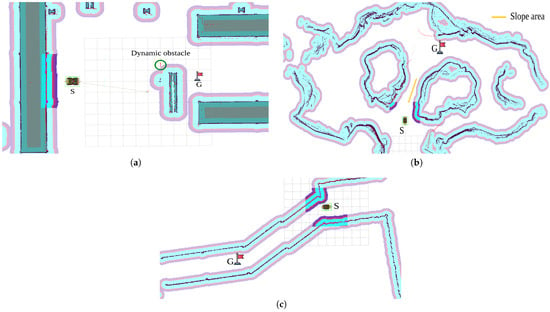
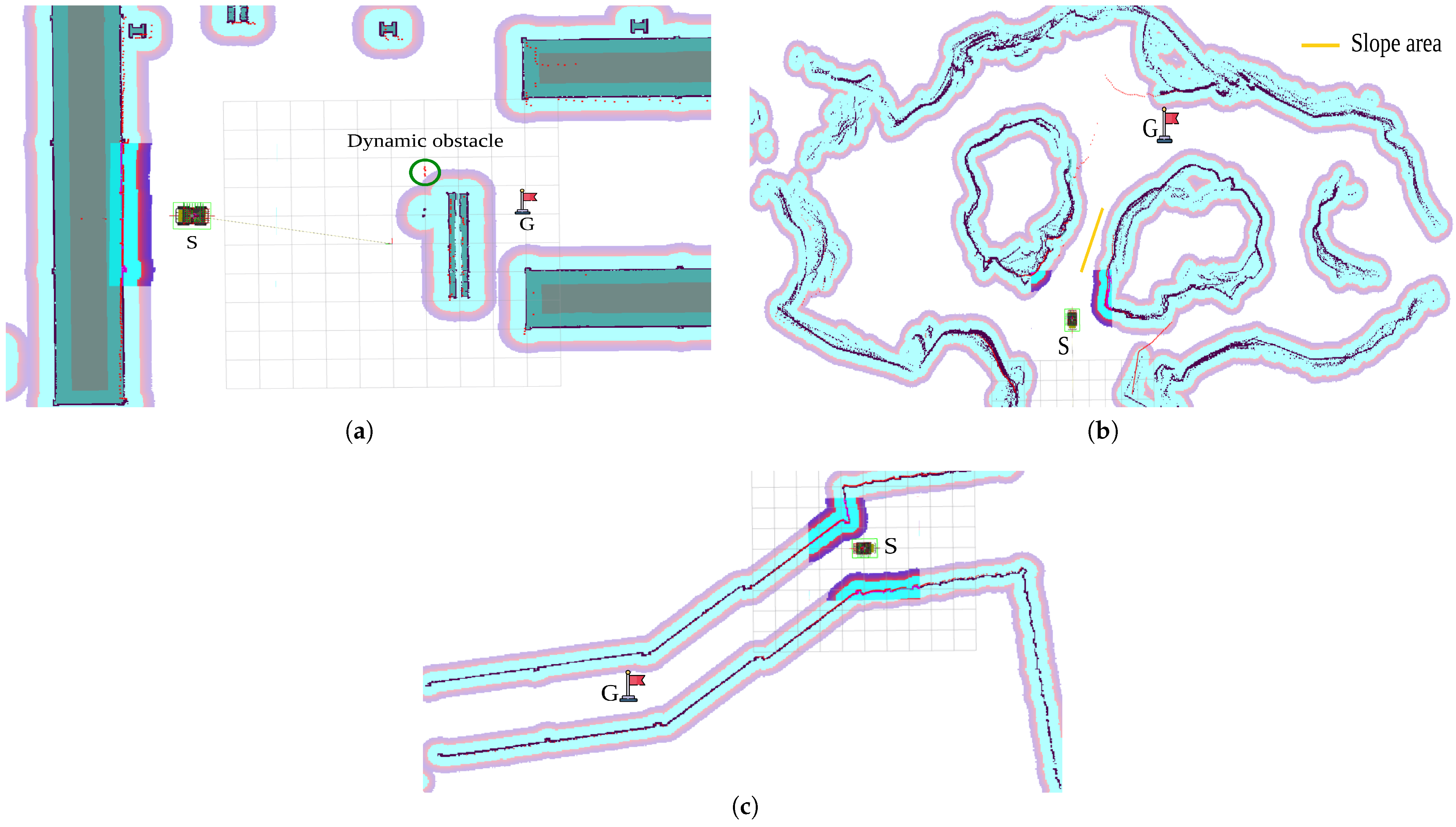
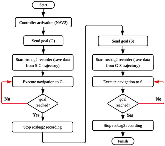
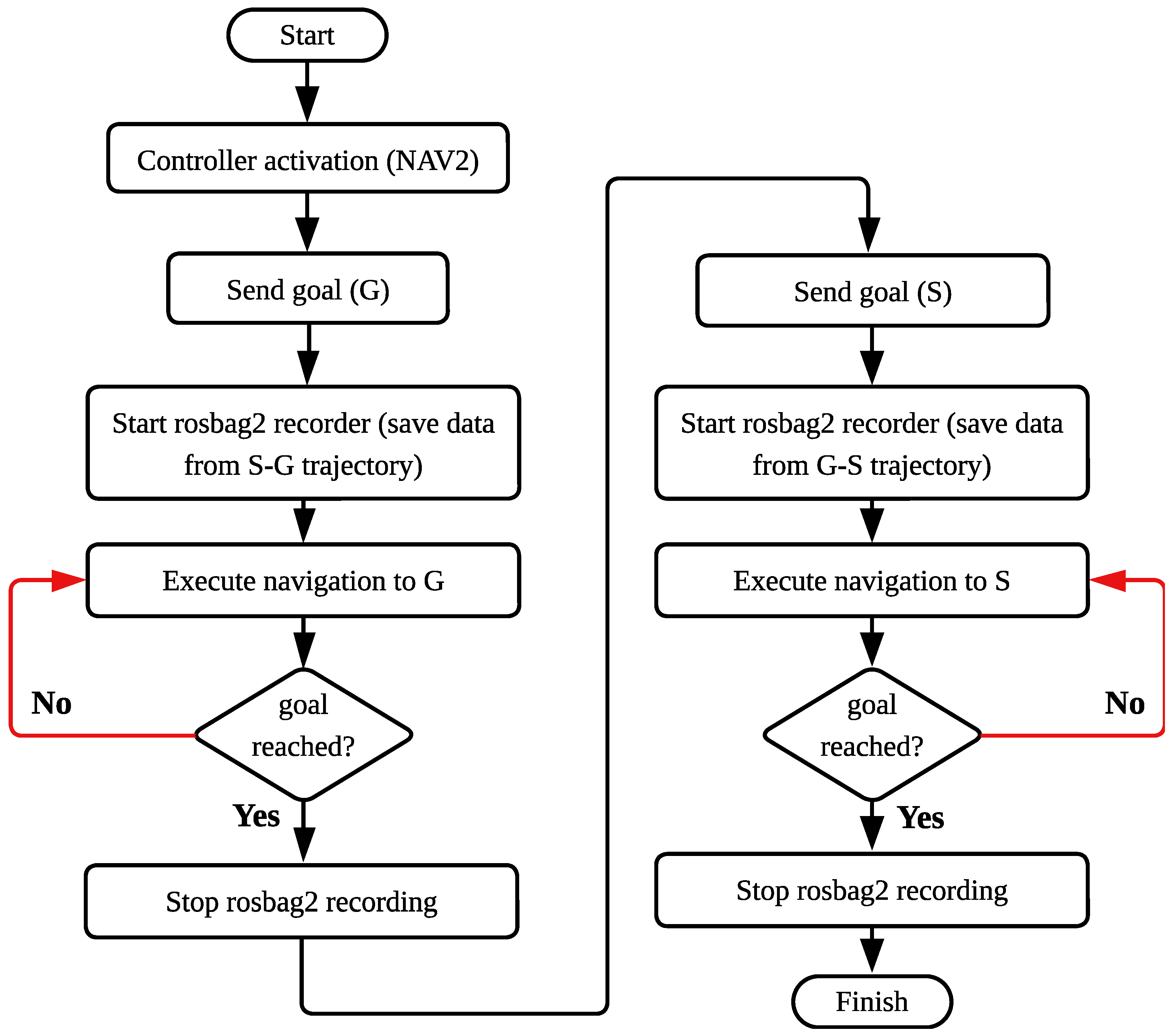
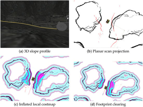
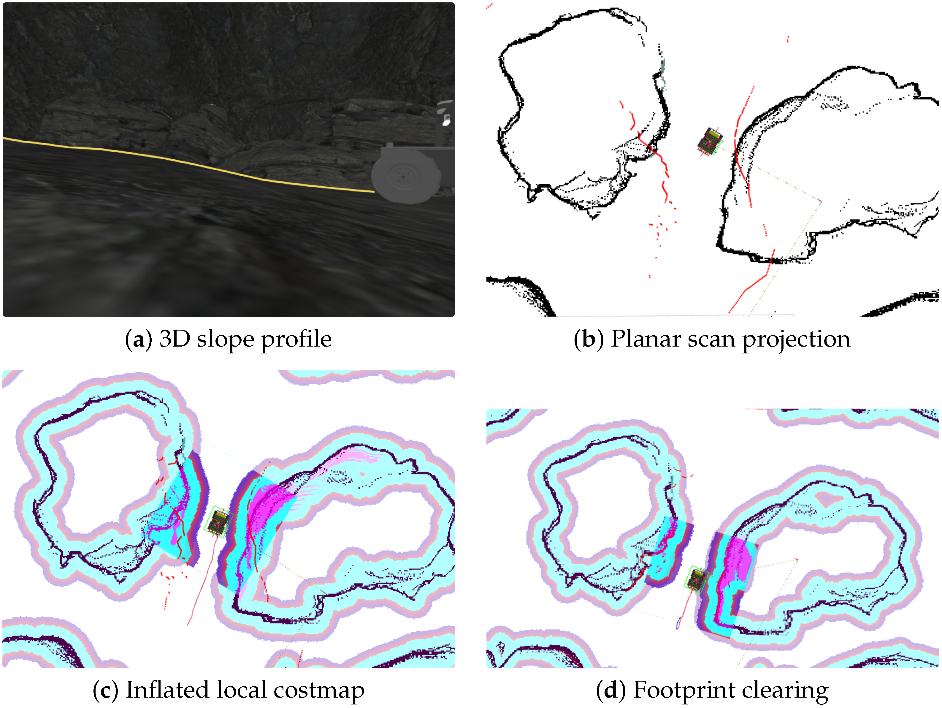
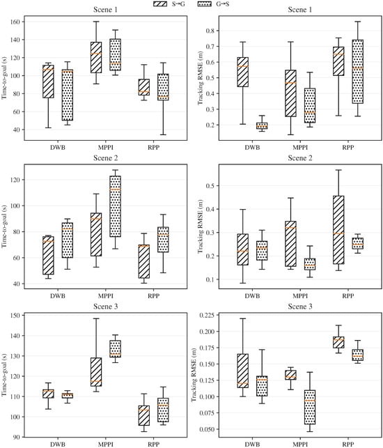
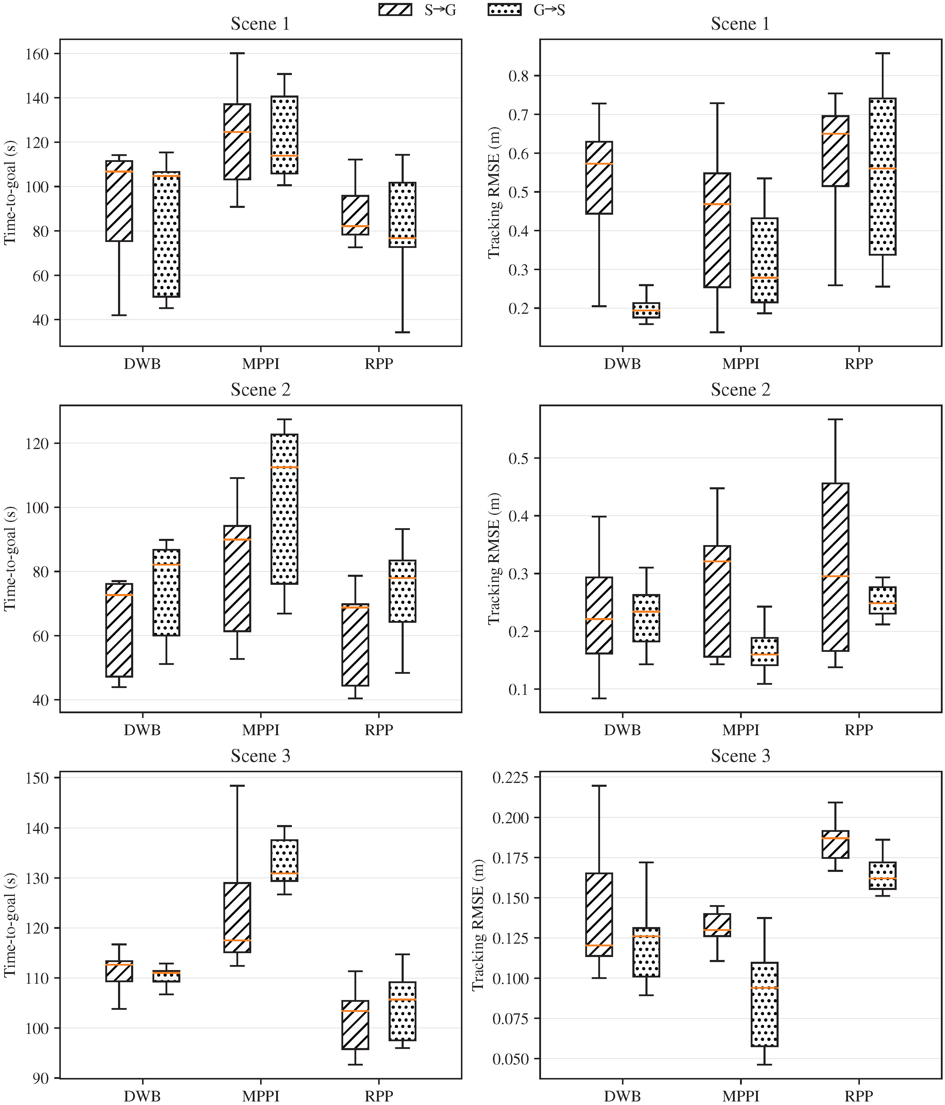
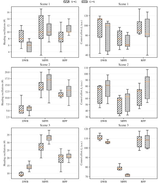
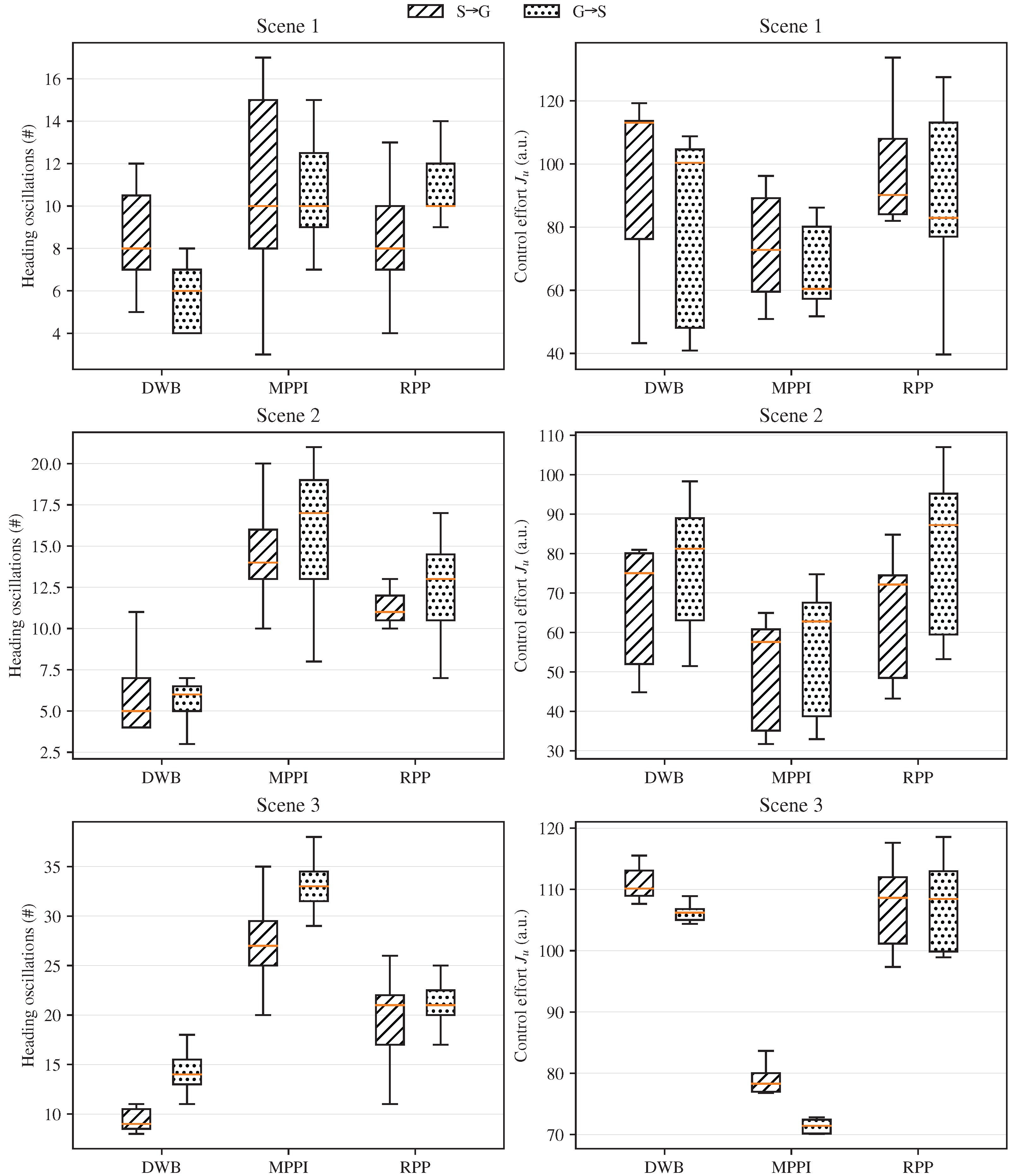
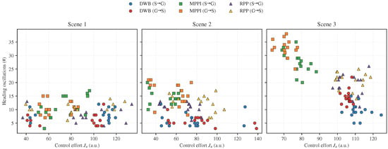
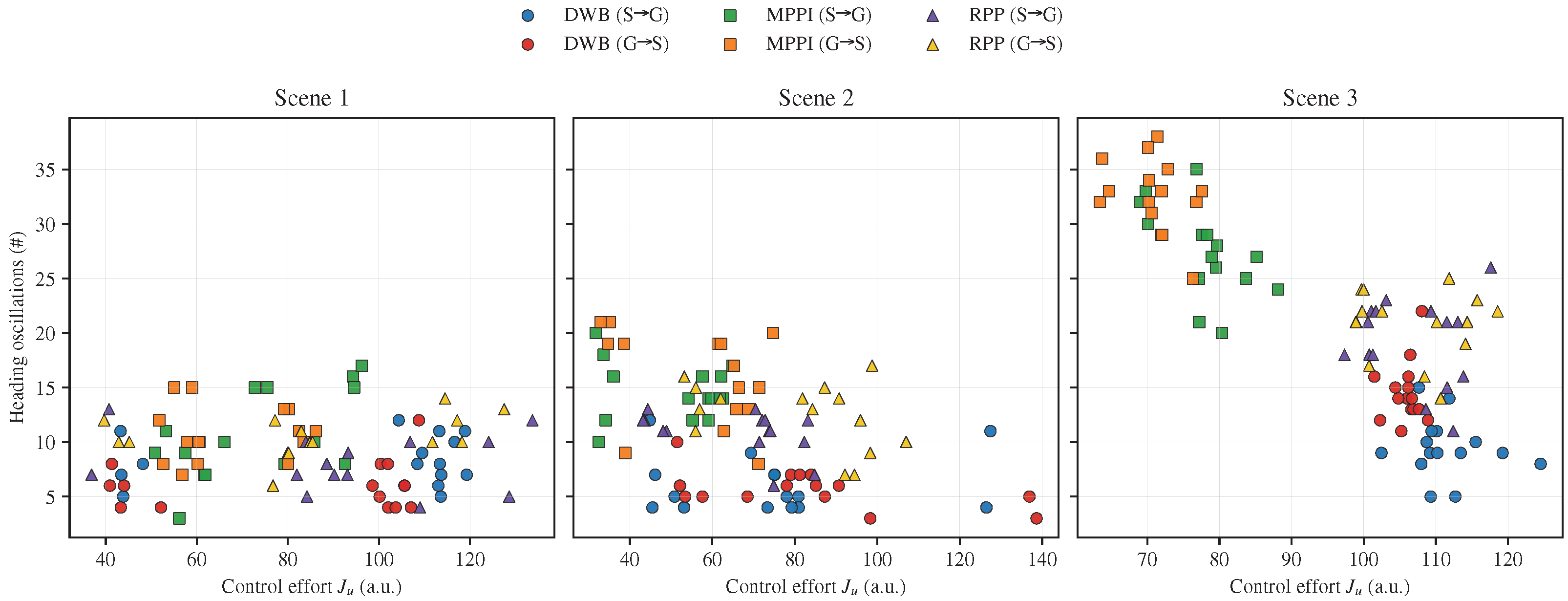

Disclaimer/Publisher’s Note: The statements, opinions and data contained in all publications are solely those of the individual author(s) and contributor(s) and not of MDPI and/or the editor(s). MDPI and/or the editor(s) disclaim responsibility for any injury to people or property resulting from any ideas, methods, instructions or products referred to in the content. |
© 2026 by the authors. Licensee MDPI, Basel, Switzerland. This article is an open access article distributed under the terms and conditions of the Creative Commons Attribution (CC BY) license.