Influence of Soil–Structure Interface Modeling on Seismic Response of Buried Nuclear Facilities in Non-Bedrock Sites

Highlights

What are the main findings?

• A three-dimensional ANSYS soil–structure interaction model compares node-to-node bonded connection, multi-point constraints and separable contact element interface methods for a buried nuclear power plant.
• The separable contact element model amplifies the soil response near the structure, while the node-to-node bonded connection model and multi-point constraint model restrain it.
• The separable contact element model yields a markedly larger structural seismic response than node-to-node bonded connection model or multi-point constraint model.
• Under the separable contact elements model, soil displacement consistently exceeds the structural displacement.

What are the implications of the main findings?

• The soil–structure interface choice strongly affects non-bedrock nuclear power plant results.
• Interface modeling must be tailored to the soil layer and site conditions.
• Findings guide connection-method selection for buried nuclear facility design.

Abstract

In this study, the seismic response of the buried structure of a nuclear power plant (NPP) located on a non-bedrock site is investigated using a three-dimensional finite element model incorporating soil–structure interaction (SSI). Three distinct soil–structure connection methods are compared: node-to-node bonded connection (NNBC), multi-point constraints (MPCs), and separable contact elements (SCEs). The results indicate that the NNBC and MPC models show a restraining effect of the structure on the seismic response of the surrounding soil, whereas the SCE model amplifies the soil response adjacent to the structure and yields significantly greater structural responses. Quantitatively, relative to the NNBC model, the SCE model increases the mean ground-surface and mean in-structure peak spectral accelerations by about 23% and 93%, with a peak soil–structure relative displacement of 0.81–0.98 cm. This study concludes that the choice of soil–structure connection method significantly influences the finite element simulation results for non-bedrock sites. Further research is needed to determine the appropriate connection methods for different soil layers.

1. Introduction

In recent years, the continuous rise in global energy demand has led to a growing gap in power supply. Nuclear power, as an efficient and clean energy source, can not only help reduce greenhouse gas emissions but also compensate for the energy shortfall, thus holding significant importance for development. Earthquakes represent one of the primary external threats to the safe operation of nuclear power plants. Lessons from past seismic-induced nuclear accidents [1] indicate that damage to nuclear power equipment during earthquakes is a major factor leading to safety incidents such as nuclear leakage. In inland areas, the availability of bedrock sites is relatively limited, increasing the likelihood of nuclear power plants being constructed on non-bedrock sites. Therefore, it is worthwhile to study the seismic response of nuclear power equipment on non-bedrock sites. Unlike bedrock sites, where seismic waves act directly on the structure, non-bedrock sites require analysis using soil–structure interaction (SSI) models. SSI is generally considered to produce two principal effects: kinematic interaction and inertial interaction [2,3]. However, analytical results for SSI problems vary depending on the specific methodology and scenario employed. There remains ongoing debate regarding whether the inclusion of SSI in simulations increases or decreases the seismic response of structures [4,5]. Destructive earthquakes—including the 1999 Chi-Chi (Taiwan), 2011 Tohoku (Japan) and 2023 Kahramanmaras (Turkiye) events—have repeatedly demonstrated that local soil conditions and soil–structure interaction (SSI) can amplify seismic demand and alter the failure mode of engineered structures [6]. The key issue, in the view of this study, lies in the contact connection between the soil and the structure. Consequently, the focus of this paper is on utilizing finite element technology to investigate soil–structure connection modeling methods suitable for the seismic analysis of nuclear power facilities.

Many scholars have conducted relevant research on the seismic resistance of nuclear power plants on non-bedrock sites using finite element simulations from both the time domain and frequency domain perspectives. Tuñón-Sanjur et al. [7] employed ANSYS and SASSI software to perform finite element simulations for the seismic analysis of AP1000 nuclear island structures on both soil and rock sites. The study introduced a lumped-mass stick model, a coarse solid-shell element model for hard rock sites, and a refined solid-shell element model for SSI analysis on soil sites, concluding that these three models yield similar seismic responses within the frequency range of 2–20 Hz. Navjeev Saxena and D.K. Paul [8,9] used a two-dimensional finite element model to analyze the sliding and separation of reactor buildings under seismic-induced soil–structure interaction. Chandrakanth Bolisetti [10] investigated structure–soil–structure interaction (SSSI) within a cluster of buildings. Both experimental and simulation results indicated that SSSI affects the structural responses. The study also compared results from the frequency-domain program SASSI and the time-domain program LS-DYNA, noting that for linear analyses, SASSI’s frequency-domain results closely match those from direct time-domain methods, whereas significant differences arise in nonlinear time-domain SSI analyses compared to linear frequency-domain outcomes. Naserkhaki [11] used a discrete soil model to analyze twin buildings, showing that SSI lengthens periods and increases lower-story drifts/shears. For closely spaced twins, SSSI partially offsets SSI effects, acting as a mild shield. Impacts were significant for soft–stiff soils but faded in hard soils. Reza V. Farahani [12] used the SASSI program to study structural responses under high-frequency seismic excitations across different geological conditions, highlighting the considerable influence of both geology and input frequency on vibrational response. Wang [13] established a numerical model considering SSI to analyze the underground station–soil–ground building system. The study highlighted the reciprocal influence between the subway station and adjacent buildings, revealing that the vertical acceleration response of the coupled system under seismic loading is significant and must be considered in design. Fernanda de Borbón [14] developed a 3D SSI finite element model of the CAREM-25 nuclear plant using ANSYS, incorporating equivalent linear soil behavior and viscous boundaries at the sides and bottom of the soil domain. The direct method was applied to investigate the influence of soil parameters on the dynamic response in SSI analysis. Abell [15] employed the Domain Reduction Method (DRM) to couple a full 3D seismic wave field—generated via finite-difference simulation of near-field dip-slip sources—with a high-fidelity finite element model of a generic nuclear power plant and layered soil site. By contrasting this approach against conventional 1-D and 3 × 1-D vertically propagating plane-wave approximations derived from the same free-field motion, they demonstrated that neglecting 3D wave-field effects can overestimate structural response peaks by approximately 50%. Utilizing a hybrid FK-FEM framework, Ba [16] developed a method capable of simulating the full seismic chain from point-source dislocation to underground structural response. This approach effectively incorporates source and propagation path effects, overcoming the limitations of uniform wave field inputs. Liang Li [17] studied multi-unit nuclear power plants on a shared foundation, establishing a detailed 3D finite element model in Abaqus to compare seismic responses considering SSI and SSSI. Results showed significant differences in floor response spectra peaks, though peak acceleration differences were relatively small. Research trends are shifting toward high-fidelity 3D modeling. Moreover, given its ability to provide more detailed information and accommodate nonlinear analysis, time-history analysis is increasingly adopted.

Post-earthquake reconnaissance and site-specific analyses of the 2023 Kahramanmaras earthquakes showed that soft soil sites systematically increased spectral demand relative to rock sites [6], and site-specific response spectra and accelerograms for bedrock versus soil surfaces have been derived [18]. Nonlinear soil–structure interaction formulations [19] and interface sliding experiments [20] further confirm that interface behavior and tangential slip control the transmitted demand.

In studies of the seismic response of SSI models on non-bedrock sites, the contact modeling between soil and structure is crucial. H. Huo [21] used 2D finite element analysis to investigate the seismic response of Daikai Station, comparing three interface friction coefficients (μ = 0, 0.4, and no-slip). The study concluded that the relative stiffness between the structure and soil, and the frictional characteristics of the interface, are key factors determining structural response under seismic loading. Farghaly [22] employed a multi-linear Winkler spring-dashpot system in three directions to model the soil–foundation interaction within SAP2000. Their analysis demonstrated that incorporating this flexible soil–structure connection significantly lengthened the fundamental period of the structure and amplified top displacements. Yikun Liu [23] performed 3D finite element SSI simulations using hard contact in the normal direction and a friction coefficient of 0.4 in the tangential direction, validating the results against experimental data. Hui Boyi [24] investigated the influence of different soil-structure contact models on the seismic response of underground structures in sites with liquefiable interlayers. Using 2D time-history analysis, the study compared tied contact, friction contact with zero thickness, and thin-layer contact with finite thickness, concluding that the finite-thickness interface model yields results closer to actual seismic responses. Liu [25] employed shaking table tests and a validated finite element model to investigate SSI effects. Their numerical approach, which utilized surface-to-surface contact to simulate the soil–pile interface, demonstrated that SSI significantly alters the system’s dynamic characteristics by reducing the fundamental frequency and increasing damping. Dou [26] established a three-dimensional finite-difference numerical model of a soil–pile–group-superstructure system in a liquefiable site using FLAC3D software. The study defined soil–pile interfaces with coupling springs, added a tip bearing spring, and modeled the pile–cap connection as an articulated link. The seismic responses showed good agreement with the results from large-scale shaking-table experiments. These findings indicate that the choice of soil–structure contact model significantly affects computational results. However, there are very few studies using three-dimensional models to investigate the differences in the time-domain and frequency-domain responses of structures caused by different soil–structure connection methods under seismic conditions. Therefore, this paper considers SSI and employs a three-dimensional finite element model to analyze the influence of the node-to-node bonded connection (NNBC), multi-point constraint (MPC), and separable contact element (SCE) models on the seismic assessment of non-bedrock buried nuclear power plants (NPPs).

The remainder of this paper is organized as follows: Section 2 describes the structural configuration and site conditions; Section 3, the finite element model, equivalent-linear soil and viscous-spring boundary; Section 4, the seismic input and equivalent boundary loading; Section 5, the responses of the ground, structure and interface for the three connection methods; Section 6 discusses these findings together with the limitations of the modeling assumptions; and Section 7 presents the conclusions. Unlike previous studies that fix a single connection type, this work compares bonded (NNBC), constraint-based (MPC) and separable frictional-contact (SCE) interfaces within a single three-dimensional time-domain model.

2. Structural Configuration and Site Condition

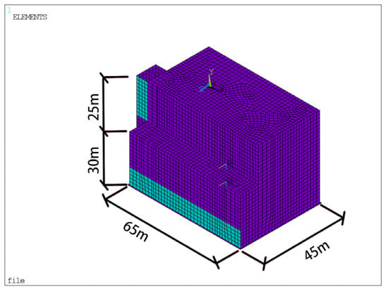
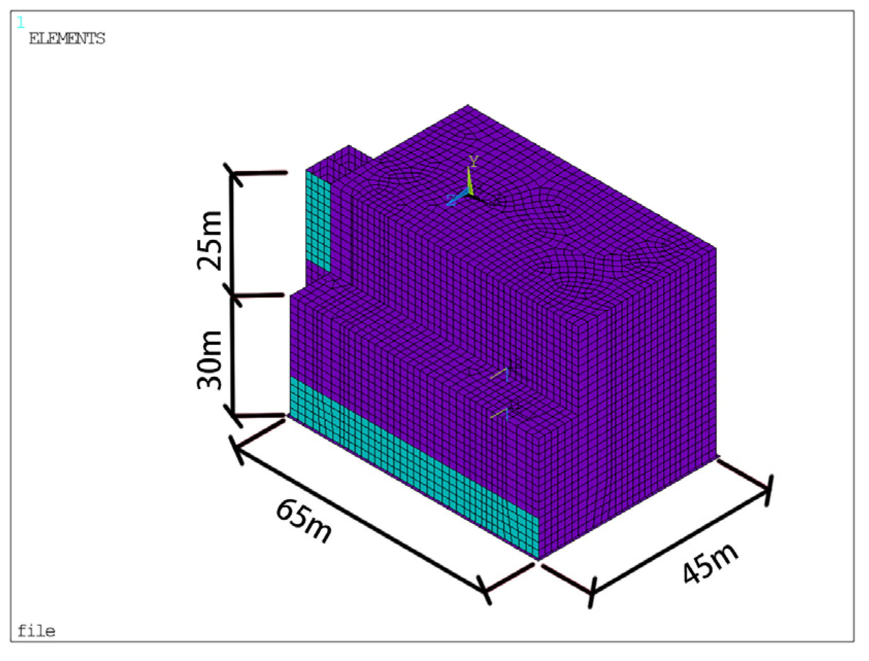
The novel buried NPP examined in this study is a small modular reactor design with its primary structures situated underground, forming a box-shaped underground configuration. The structure has a burial depth of 30 m and an above-ground height of 25 m, with plan dimensions of approximately 65 by 45 m. This configuration results in dynamic characteristics that are more representative of an underground structure, making its behavior markedly different from that of a conventional, large-scale surface NPP.

The subsurface conditions to a depth of 50 m below the plant consist primarily of gravelly sandstone. This material is classified as a semi-igneous rock, representing a transitional state between soil and rock. Below this layer lies strongly weathered granite. The gravelly sandstone layer exhibits a shear wave velocity ranging from 250 m/s to 750 m/s, a dynamic elastic modulus of 0.36 GPa, and a dynamic shear modulus of 0.13 GPa. The value G = 0.13 GPa quoted above is the small-strain dynamic shear modulus of the gravelly sandstone as provided by the geotechnical investigation, whereas the layer-wise shear moduli in Table 1 (98–1373 MPa) are the strain-compatible equivalent-linear values obtained after iteration in the one-dimensional site response analysis, with the corresponding shear-wave velocities in Table 1 computed as Vs = (G/rho)^0.5 from these moduli and the layer densities; the two therefore refer to different strain levels and are not inconsistent. The layer densities (1901–2145 kg/m³) and Poisson’s ratios (0.33–0.39) used in the equivalent-linear model are listed in Table 1.

Table 1. Properties of soil profiles.

Soil Layer	Depth (m)	Shear Wave Velocity (m/sec)	Shear Modulus (Mpa)	Damping Ratio (%)	Mass-Proportional Damping	Stiffness-Proportional Damping	Density (kg/m3)	Poisson’s Ratio
1	0~9	226	98	7.50	2.64	0.00202	1923	0.38
2	9~18	324	202	7.62	3.05	0.00162	1930	0.39
3	18~27	416	329	7.70	3.30	0.00136	1901	0.36
4	27~37	545	566	5.40	2.37	0.000897	1905	0.36
5	37~47	667	855	4.48	2.04	0.000647	1929	0.34
6	47~55	800	1373	3.44	1.59	0.000471	2145	0.33

3. Finite Element Model

To address the needs for nonlinear analysis and to obtain results in both the time and frequency domains [27,28], a three-dimensional soil–structure interaction (SSI) finite element model is developed in this study. The modeling and analysis are conducted using the finite element software ANSYS 2022 R1.

3.1. Model of the Structure

The primary containment and reactor building, situated centrally within the NPP, are constructed with thick reinforced concrete shear walls and slabs. Given the model’s complexity, shell elements were selected over solid elements for the structural modeling, offering a lower computational cost without compromising result accuracy. These shell elements employ a linear shape function. Quadrilateral elements with four nodes and six degrees of freedom per node were used. Specifically, within the ANSYS environment, the SHELL63 element was used for walls, and the BEAM188 element was used for beams and columns. An element size of 1.0 m was adopted, yielding a sufficiently refined mesh for the study’s objectives. The final structural model comprised 11,591 elements and 10,637 nodes, shown in Figure 1.

Figure 1. Model of the structure.

The element size of 1.0 m was selected with reference to the shortest shear wavelength of interest. In the softest layer, the strain-compatible (post-iteration) shear-wave velocity is 226 m/s (Table 1), giving a wavelength of about 6.8 m at 33 Hz, i.e., about seven elements per wavelength, so the one-eighth-wavelength criterion [29] is satisfied for frequencies up to about 28 Hz; at the site dominant frequency (about 5 Hz), there are about 45 elements per wavelength. The analysis is a single implicit transient (ANTYPE, TRANS) solution with a fixed time step dt = 0.01 s over 2570 load steps using the default Newmark constant-average-acceleration scheme; the structure uses SHELL63 and BEAM188, the soil SOLID45, and SURF154 elements carry the equivalent boundary loads.

The concrete behavior was represented using a linear isotropic elastic material model, with a Young’s modulus of 35 GPa, a Poisson’s ratio of 0.2, and a density of 2600 kg/m³.

The concrete is modeled as linear isotropic elastic because the design-basis motion is expected to keep the containment essentially elastic; this precludes capturing cracking or inelastic energy dissipation in the structure.

3.2. Model of Soil

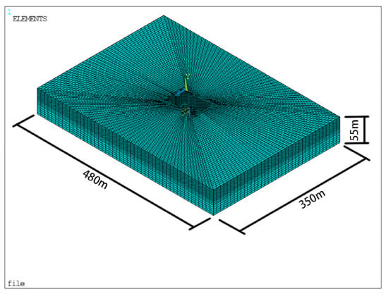
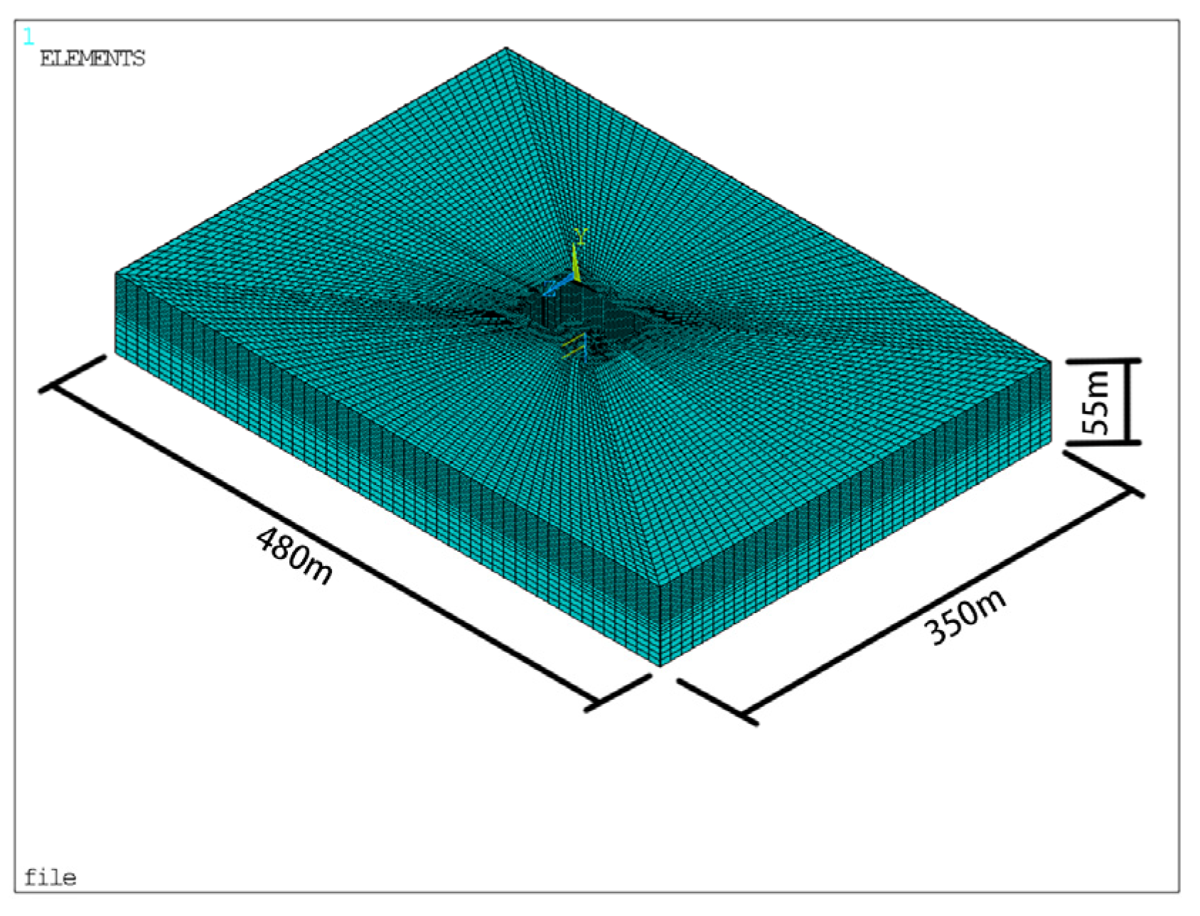
Soil nonlinearity was approximated using equivalent linear properties. A 3D soil domain was modeled with hexahedral solid elements featuring a linear shape function, 8 nodes, and 3 degrees of freedom per node. In accordance with code requirements [30], the distance from the model boundary to the structural edge shall exceed three times the structural width. The soil model dimensions are 480 m in length, 350 m in width, and 55 m in depth. The mesh was refined similarly to the structural mesh near the interface and coarsened progressively towards the model boundaries. The SOLID45 element was utilized for the soil, resulting in a model with 191,724 elements and 203,595 nodes, shown in Figure 2.

Figure 2. Model of the soil.

Soil properties were stratified vertically. The dynamic properties for each layer were determined iteratively based on one-dimensional seismic site response analysis.

To account for soil nonlinearity, the one-dimensional site response was performed using an equivalent-linear approach, as implemented in programs like SHAKE and EERA. This method simulates soil nonlinearity under seismic loading by employing a hysteretic damping ratio and a shear modulus that degrade with increasing shear strain. The equivalent soil parameters (shear modulus and hysteretic damping) are iteratively adjusted until compatible with the effective shear strain levels. The final equivalent parameters, representing the soil’s nonlinear response, are then used in the SSI analysis. While the degraded shear modulus is directly applicable, the hysteretic damping must be converted for use in the time-domain analysis. This conversion was achieved by approximating the hysteretic damping as Rayleigh damping, following the method in [31]. This scheme equates the hysteretic damping coefficient of a soil layer to its modal damping ratio within the Rayleigh damping model. The mass and stiffness proportional coefficients for the Rayleigh damping are then calculated based on the site’s fundamental frequency and the dominant frequency of the input motion, ultimately forming a linear elastic model with Rayleigh damping for the site response calculation. Properties of soil profiles are presented in Table 1.

3.3. The Viscous-Spring Artificial Boundary

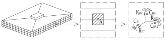
The analysis of seismic SSI problems requires defining a finite computational domain. To simulate the unbounded soil medium, artificial boundary conditions that absorb outgoing waves are applied at the truncated model boundaries. This study employs the viscous-spring boundary condition [32], recognized for its stability, accuracy, and effectiveness in simulating the radiation damping and elastic recovery of a semi-infinite domain. As schematically illustrated in Figure 3 [32], this boundary condition is implemented by applying parallel spring–damper systems in three orthogonal directions to the nodes on the model’s lateral and bottom boundaries.

Figure 3. SSI model with viscous-spring boundary.

The parameters of the springs and dampers are as follows [32]:

Normal direction:

$$K_{\mathit{BN}}={\displaystyle \frac{{\alpha }_{N}G}{R}}A,C_{\mathit{BN}}=\rho c_{p}A$$

(1)

Tangential direction:

$$K_{\mathit{BT}}={\displaystyle \frac{{\alpha }_{T}G}{R}}A,C_{\mathit{BT}}=\rho c_{s}A$$

(2)

Of these parameters, K_BN denotes the spring coefficient of Normal direction, and K_BT denotes the spring coefficient of Tangential direction. C_BN represents the damping coefficient of Normal direction and C_BT represents the damping coefficient of Tangential direction. The shear modulus of the material is given by G, and its mass density is denoted by ρ. The propagation velocities of the shear wave and the compression wave are defined as c_s and c_p, respectively. Furthermore, α_N and α_T are the modified coefficients specified for the normal and tangential directions of the boundary. Finally, the variable R is defined as the radial distance from the artificial boundary to the geometric center of the finite element model.

The existing viscoelastic artificial boundary is typically simulated using discrete spring–dashpot analogs. However, when addressing three-dimensional problems with finite element models, this method can be computationally intensive and time-consuming. Therefore, this study adopts a consistent viscous-spring boundary, which yields results essentially consistent with the discrete viscoelastic artificial boundary while enabling more convenient and rapid computation [33]. The implementation of the consistent viscous-spring boundary involves adding a layer of solid elements to the outer sides of the soil domain, whose material properties are specifically defined to replicate the mechanical characteristics of the springs and dashpots.

The parameters of the consistent viscous-spring artificial boundary are as follows:

$$\tilde{G}=h{K}_{\mathit{BT}}$$

(3)

$$\tilde{E}={\displaystyle \frac{(1+\tilde{\upsilon })(1-2\tilde{\upsilon })}{1-\tilde{\upsilon }}}h{K}_{\mathit{BN}}$$

(4)

$$\tilde{\upsilon }=\left\{\begin{array}{c}{\displaystyle \frac{\alpha -2}{2(\alpha -1)}}\alpha \ge 2\\ \mathrm{0 }\alpha <2\end{array}\right.$$

(5)

α = α_N/α_T

(6)

$$\tilde{\eta }={\displaystyle \frac{\mathit{\rho R}}{3G}}(2{\displaystyle \frac{c_s}{{\alpha }_T}}+{\displaystyle \frac{c_p}{{\alpha }_N}})$$

(7)

where $\tilde{G}$ is the equivalent shear modulus, $\tilde{E}$ is the equivalent elastic modulus, $\tilde{\upsilon }$ is the equivalent Poisson’s ratio, and $\tilde{\eta }$ is the equivalent damping coefficient. The modified parameter α_N and α_T can be determined from analysis and some example tests [33]. The recommended value ranges are 1.0–2.0 for αN and 0.5–1.0 for αT, and the corresponding recommended values adopted in this study are 1.33 and 0.67, respectively. Of these, the equivalent damping coefficient eta-tilde is the damping parameter of the added consistent viscous-spring boundary layer: it reproduces the dashpot (radiation-damping) behavior of the discrete viscous-spring boundary within the boundary-layer solid elements and is implemented as their Rayleigh (stiffness-proportional) damping, following [33].

3.4. Soil–Structure Interaction

Accurately capturing the seismic response of the structure necessitates a precise simulation of the connection between the soil and the structure. This study will utilize ANSYS finite element software to develop three distinct finite element models representing different soil–structure connection methods, aiming to analyze the impact of these different connection methods on the structural response.

The first method is a NNBC, a conventional approach frequently used in seismic analysis. Although potential incompatibility in degrees of freedom (e.g., three DOFs per node for solid elements versus six for shell elements) may lead to an attenuation of seismic motion transfer, this method is simple to implement and computationally efficient. It is suitable for scenarios where only minor relative slippage is expected between the soil and structure, and load transfer is maintained. In the NNBC model, the three translational degrees of freedom (UX, UY, UZ) of coincident soil and structure nodes are merged; the rotational degrees of freedom of the shell nodes at the interface are not constrained by the solid nodes, which is the source of the degree-of-freedom incompatibility discussed in Section 6.

The second method involves establishing SCEs between the soil and structure to simulate potential gap opening, tangential sliding, and friction at the interface. ANSYS provides robust contact element formulations; specifically, target element TARGE170 and contact element CONTA173 can be paired to create a contact pair. This setup allows for separation and sliding between the adjacent elements on either side of the interface. The normal contact pressure reduces to zero upon separation, making this method appropriate for simulating cases where the soil and structure may lose contact.

The third method employs a bonded contact formulation with MPC. This approach binds the structural and soil elements together within a defined contact area, creating a rigid connection in both the normal and tangential directions. It enforces compatibility of displacement and rotation at the interface nodes, making it applicable for simulating conditions where the soil and structure are expected to undergo coordinated deformation without separation or significant slippage under vibrational loading. In the MPC model, the constraint equations enforce compatibility of the translational degrees of freedom between the soil solid nodes and the structure shell nodes over the contact area, removing the degree-of-freedom incompatibility present in NNBC.

4. Load

Seismic excitation in this model is applied in the form of a seismic load. The procedure for applying the seismic load is as follows. First, the surface ground motion time history suitable for the seismic check of the nuclear island structure at the specific site is obtained. Subsequently, this surface ground motion time history is used to back-calculate the corresponding seismic motion time histories at different depths within the model domain. Finally, the seismic force loads at various depths are computed based on these depth-specific seismic motion time histories and the properties of the artificial boundary.

4.1. Surface Ground Motion Time History

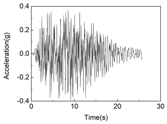
In this model, the study adopts the free-field surface ground motion parameters corresponding to a 1% probability of exceedance in 100 years at the project site, with a damping ratio of 5%. To meet the requirements stipulated by the code [30], an artificial acceleration time history that matches target design response spectrum (TDRS) and envelope target power spectral density (TPSD) was generated. For this purpose, a hybrid simulation method was employed, which is advantageous in terms of both computational accuracy and efficiency. The design motion corresponds to a peak ground acceleration of approximately 0.39 g at the free-field surface, is compatible with the site-specific target design response spectrum (TDRS) with 5% damping, and represents a non-bedrock site (gravelly sandstone over strongly weathered granite, Vs 250–750 m/s).

The horizontal artificial acceleration time histories generated using the hybrid simulation method, corresponding to the 1% probability of exceedance in 100 years, are shown in Figure 4. The time interval for the artificial acceleration time history is Δt = 0.01 s, with a total duration of T₀ = 25.7 s.

Figure 4. Artificial acceleration time history.

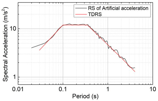
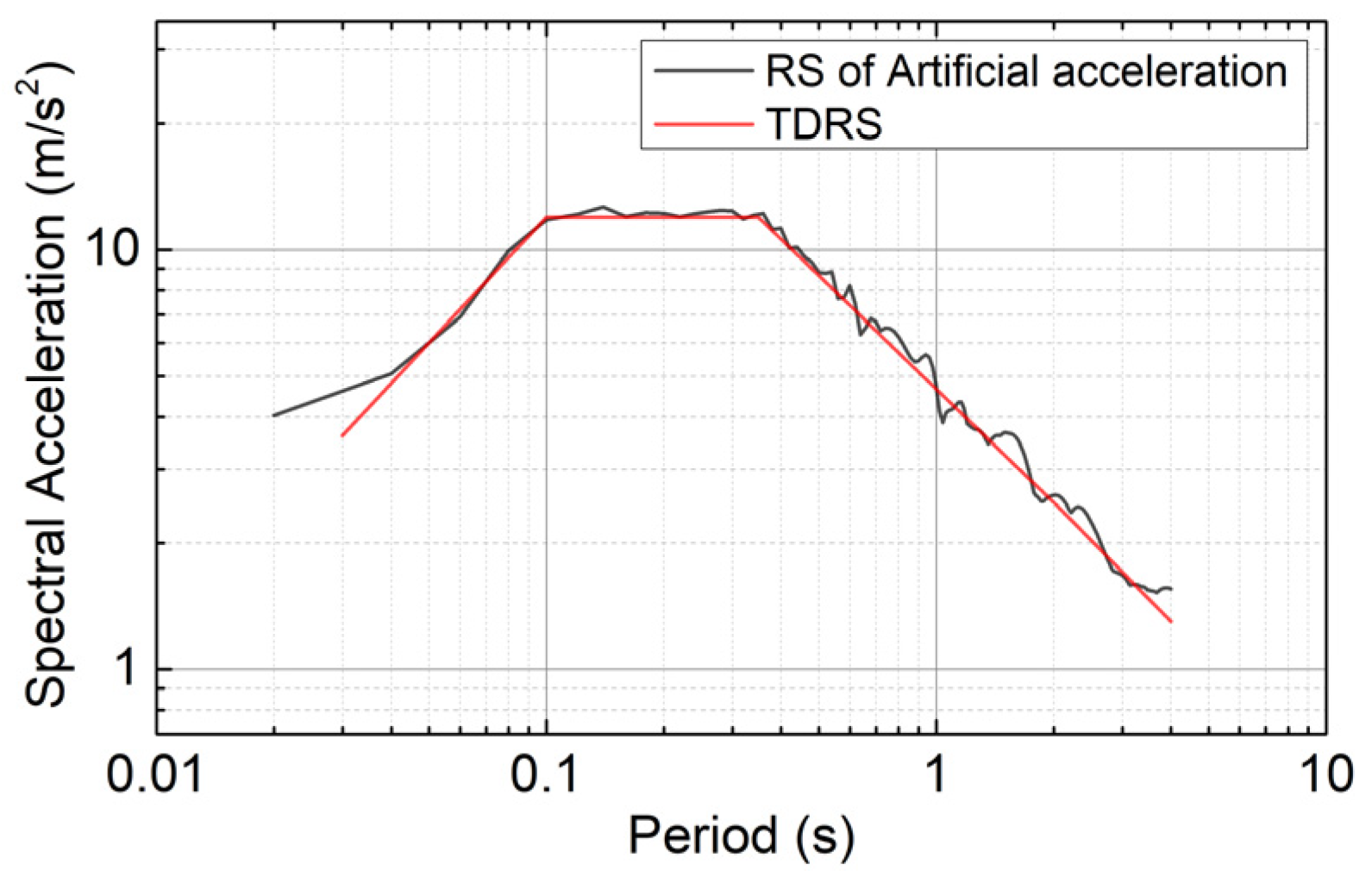
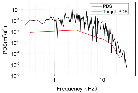
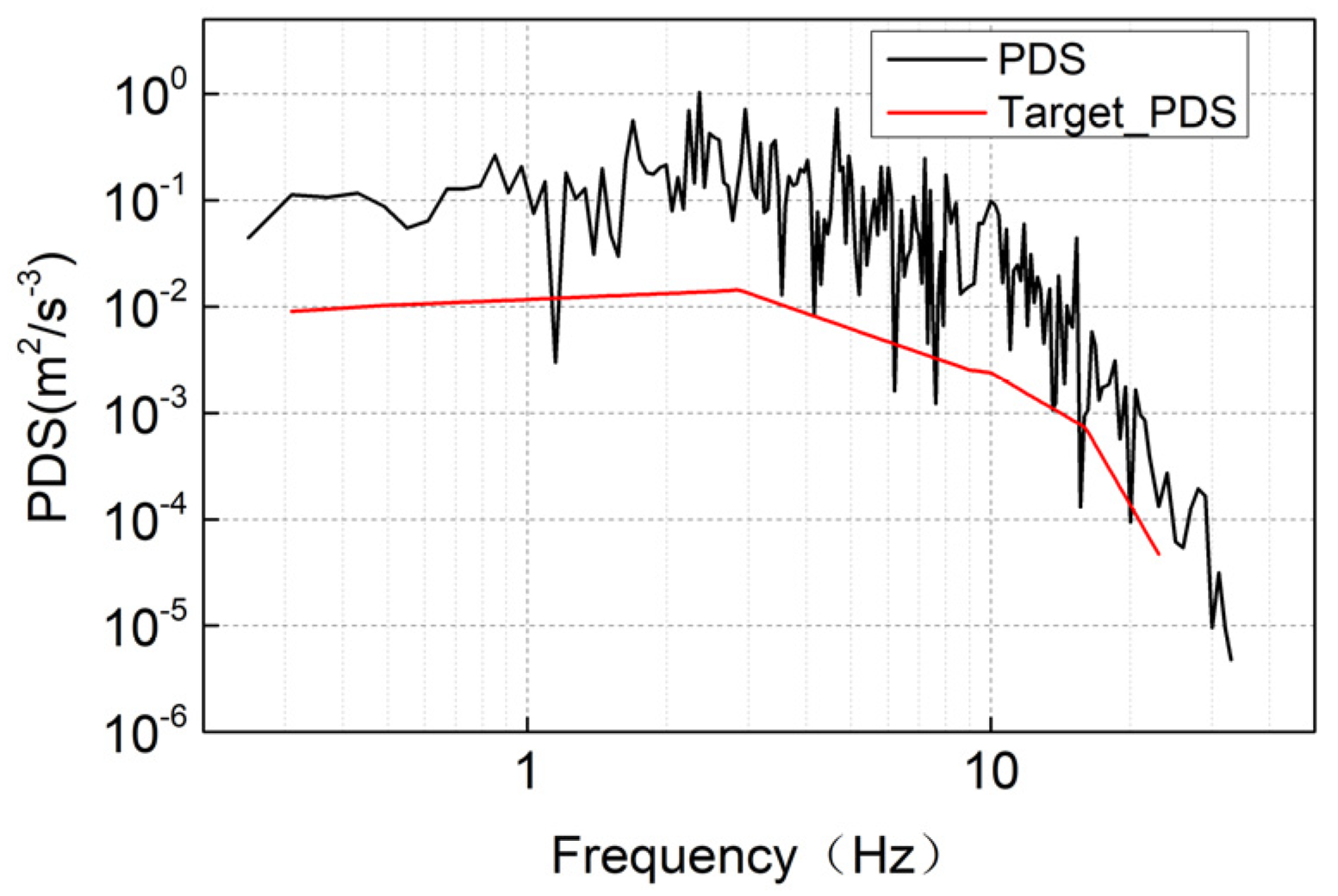
As required by the specifications [30], the number of frequency control points for the response spectrum (RS) must be no less than 75 within the frequency range of 0.2–33 Hz and no less than 100 within the range of 0.1–50 Hz. These frequency points should be approximately uniformly distributed on a logarithmic scale. In this study, the numbers of frequency control points are 111 and 120, respectively, meeting the code’s requirement [30] for frequency increment. Figure 5 and Figure 6 present the matching results between the artificial acceleration time history and the TDRS, as well as the results of enveloping 80% of the TPSD, respectively.

Figure 5. TDRS matching results of surface artificial acceleration time history.

Figure 6. TPSD envelop results of surface artificial acceleration time history.

For all frequency control points, there is only one point for each of the horizontal and vertical artificial acceleration time histories where the RS value is lower than the TDRS value. This number is within the allowable limit of no more than 5 points, and the value is not less than 90% of the TDRS. Furthermore, the RS values at all control points do not exceed 1.3 times the TDRS values [30]. For frequency control points within the range of 0.3–24 Hz, the power spectral density (PSD) of both artificial acceleration time histories exceeds the corresponding 80% TPSD values, thus satisfying the requirements of the code [30].

4.2. Seismic Responses of Different Depths in Free Field

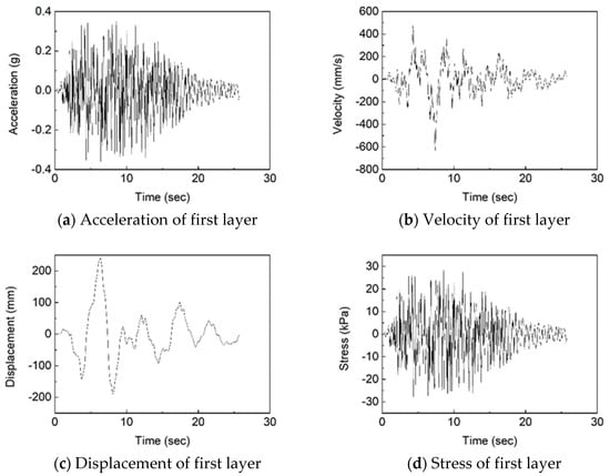
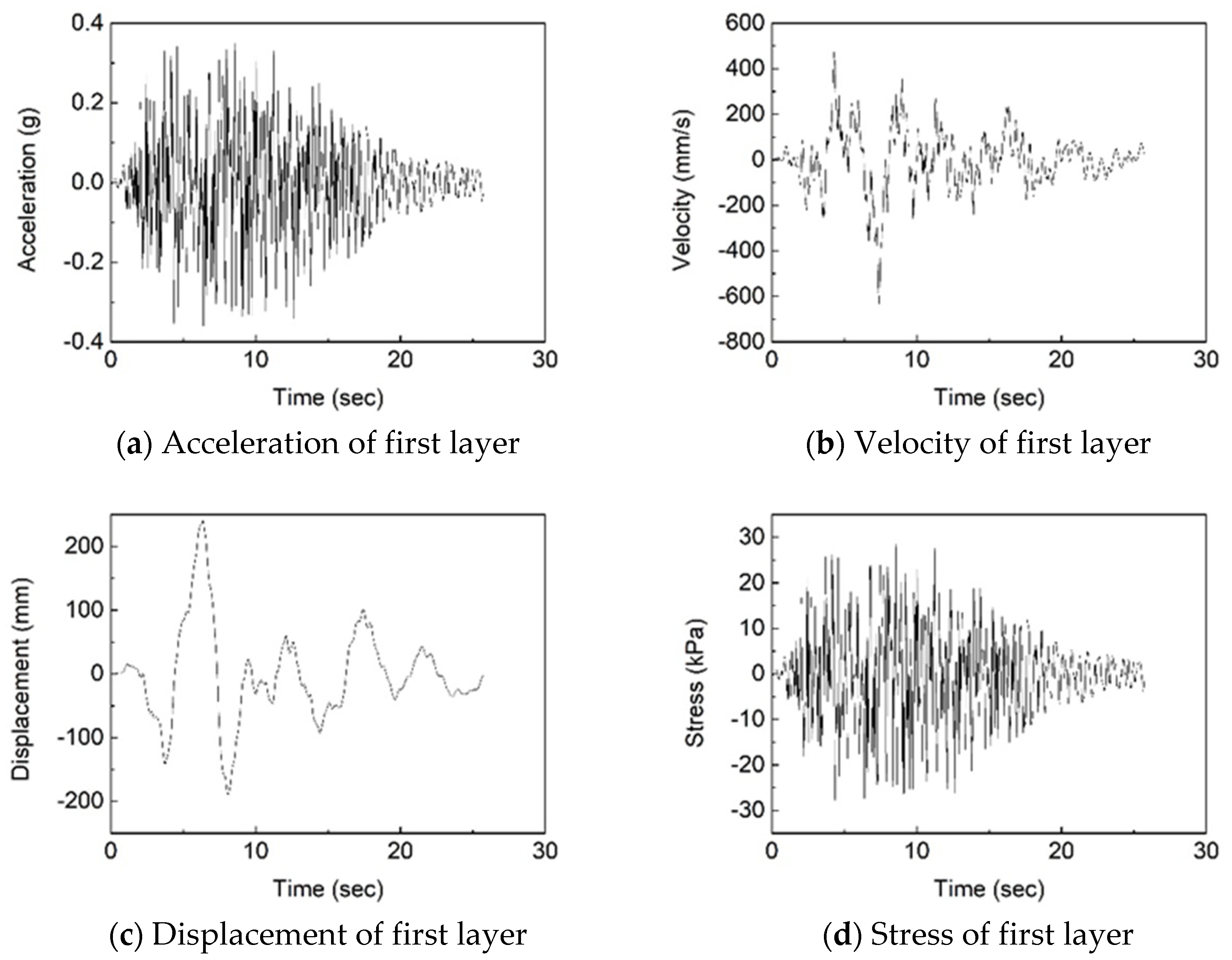
Under strong seismic motions, soil behavior is generally considered nonlinear. As the shear strain γd of the soil increases, the dynamic shear modulus ratio Gd/Gmax (where Gd is the dynamic shear modulus and Gmax is the maximum shear modulus) exhibits a decreasing trend, while the damping ratio ζ shows an increasing trend. Based on the curves describing the relationship between the dynamic shear modulus ratio, damping ratio, and shear strain, the dynamic shear modulus and damping ratio under seismic loading can be determined using the one-dimensional equivalent linearization method. Subsequently, acceleration, velocity, displacement, and stress time histories at different depths of the site are obtained through site seismic response analysis. These results are ultimately used as input conditions for the wave method. This study employs EERA software to perform the soil layer response calculation. Using the artificially generated surface acceleration time history mentioned above, the seismic response at different depths of the free field is determined, including the accelerations, velocities, displacements and shear stresses of each layer. The seismic response at the first layer (0–9 m) is shown in Figure 7.

Figure 7. Seismic response at first layer.

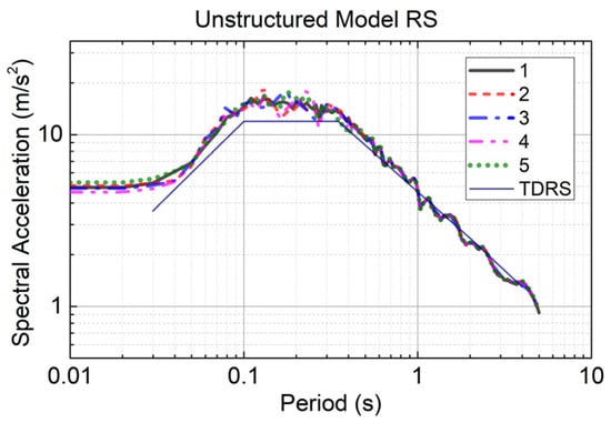
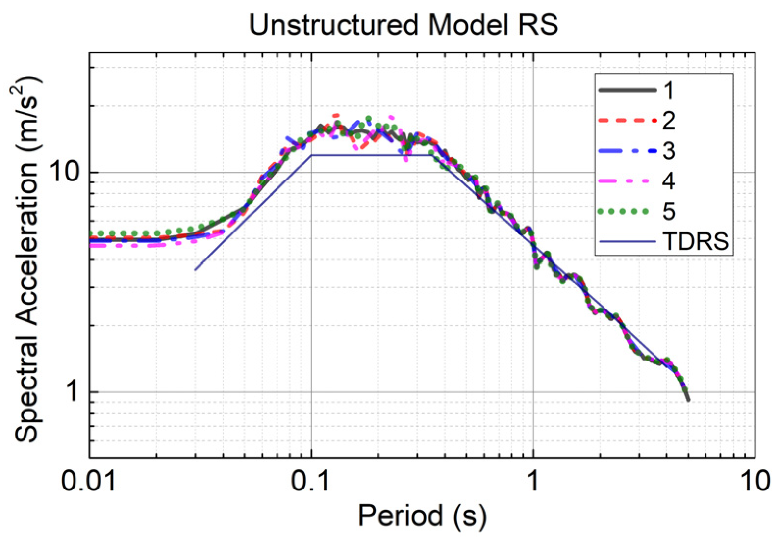
To verify the model, a free-field (no-structure) model with identical soil, domain, boundaries and input motion was analyzed. Its surface response spectra match the target design spectrum (Figure 8) over the whole period range (including T > 1 s), and the computed surface PGA (0.40–0.43 g) and peak displacement (about 0.23 m) agree with the one-dimensional equivalent-linear EERA results (0.37 g, 0.24 m) to within about 10%, confirming that the soil column, the viscous-spring boundary and the seismic input are correctly formulated.

Figure 8. Response spectrum of unstructured model.

4.3. Equivalent Seismic Force Load

Based on the relevant literature [34], the seismic action is treated as an equivalent load applied to the artificial boundaries to achieve the input of ground motion. The artificial boundaries define a finite computational domain extracted from the semi-infinite free field. The equivalent stress time history applied to the interior faces of these artificial boundaries should ensure that the displacements and stresses on the boundaries are consistent with those of the original free field. The formulation is as follows [34]: the equivalent-boundary-load formulation (Equations (10)–(12)) is taken from [34]; the authors’ own contribution lies in combining this formulation with the consistent viscous-spring boundary of Section 3.3 and in driving it with the free-field displacement, velocity and stress fields computed by EERA for the present non-bedrock site.

$$\mathsf{\delta }\left({\mathrm{x}}_{\mathrm{B}},{\mathrm{y}}_{\mathrm{B}},{\mathrm{z}}_{\mathrm{B}},\mathrm{t}\right)={\mathsf{\delta }}_0\left({\mathrm{x}}_{\mathrm{B}},{\mathrm{y}}_{\mathrm{B}},{\mathrm{z}}_{\mathrm{B}},\mathrm{t}\right)$$

(8)

$$\mathsf{\tau }\left({\mathrm{x}}_{\mathrm{B}},{\mathrm{y}}_{\mathrm{B}},{\mathrm{z}}_{\mathrm{B}},\mathrm{t}\right)={\mathsf{\tau }}_0\left({\mathrm{x}}_{\mathrm{B}},{\mathrm{y}}_{\mathrm{B}},{\mathrm{z}}_{\mathrm{B}},\mathrm{t}\right)$$

(9)

In the equations, δ and τ are the displacements and stresses (with coordinates of x_B, y_B, z_B, and time t) at the internal nodes within the artificial boundary. δ₀ and τ₀ are the free-field displacements and stresses (with coordinates of x_B, y_B, z_B, and time t).

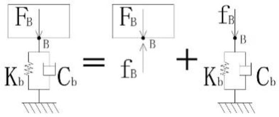
The stress F_B (t) applied at the artificial boundary point (modeled as a parallel spring-dashpot system) is assumed as the input value for wave motion. Using the concept of a free-body diagram in mechanical analysis, the artificial boundary is conceptually separated from the soil mass at the internal boundary point B, as shown in Figure 9.

Figure 9. Artificial boundaries and isolated bodies.

The internal forces f_B(t) at the junction of the physical components and the artificial boundary are shown in Figure 9. The stress at the artificial boundary is given by Equation (10).

$$\mathsf{\tau }\left({\mathrm{x}}_{\mathrm{B}},{\mathrm{y}}_{\mathrm{B}},{\mathrm{z}}_{\mathrm{B}},\mathrm{t}\right)=F_B(t)-f_B(t)$$

(10)

For the free-body diagram of the artificial boundary, the equation of motion for the physical components (comprising the spring and the dashpot) is given by Equation (11):

$$f_B(t)=C_b{\dot{\mathsf{\delta }}}_0({\mathrm{x}}_{\mathrm{B}},{\mathrm{y}}_{\mathrm{B}},{\mathrm{z}}_{\mathrm{B}},\mathrm{t})+K_b{\mathsf{\delta }}_0({\mathrm{x}}_{\mathrm{B}},{\mathrm{y}}_{\mathrm{B}},{\mathrm{z}}_{\mathrm{B}},\mathrm{t})$$

(11)

C_b and K_b are the damping coefficient of the distributed dashpot and the stiffness coefficient of the distributed spring, respectively.

Substituting Equation (11) into Equation (10) yields the following:

$$F_B(t)={\mathsf{\tau }}_0({\mathrm{x}}_{\mathrm{B}},{\mathrm{y}}_{\mathrm{B}},{\mathrm{z}}_{\mathrm{B}},\mathrm{t})+C_b{\dot{\mathsf{\delta }}}_0({\mathrm{x}}_{\mathrm{B}},{\mathrm{y}}_{\mathrm{B}},{\mathrm{z}}_{\mathrm{B}},\mathrm{t})+K_b{\mathsf{\delta }}_0({\mathrm{x}}_{\mathrm{B}},{\mathrm{y}}_{\mathrm{B}},{\mathrm{z}}_{\mathrm{B}},\mathrm{t})$$

(12)

The displacements, velocities and stresses in the free field were all calculated by EERA software.

5. Result

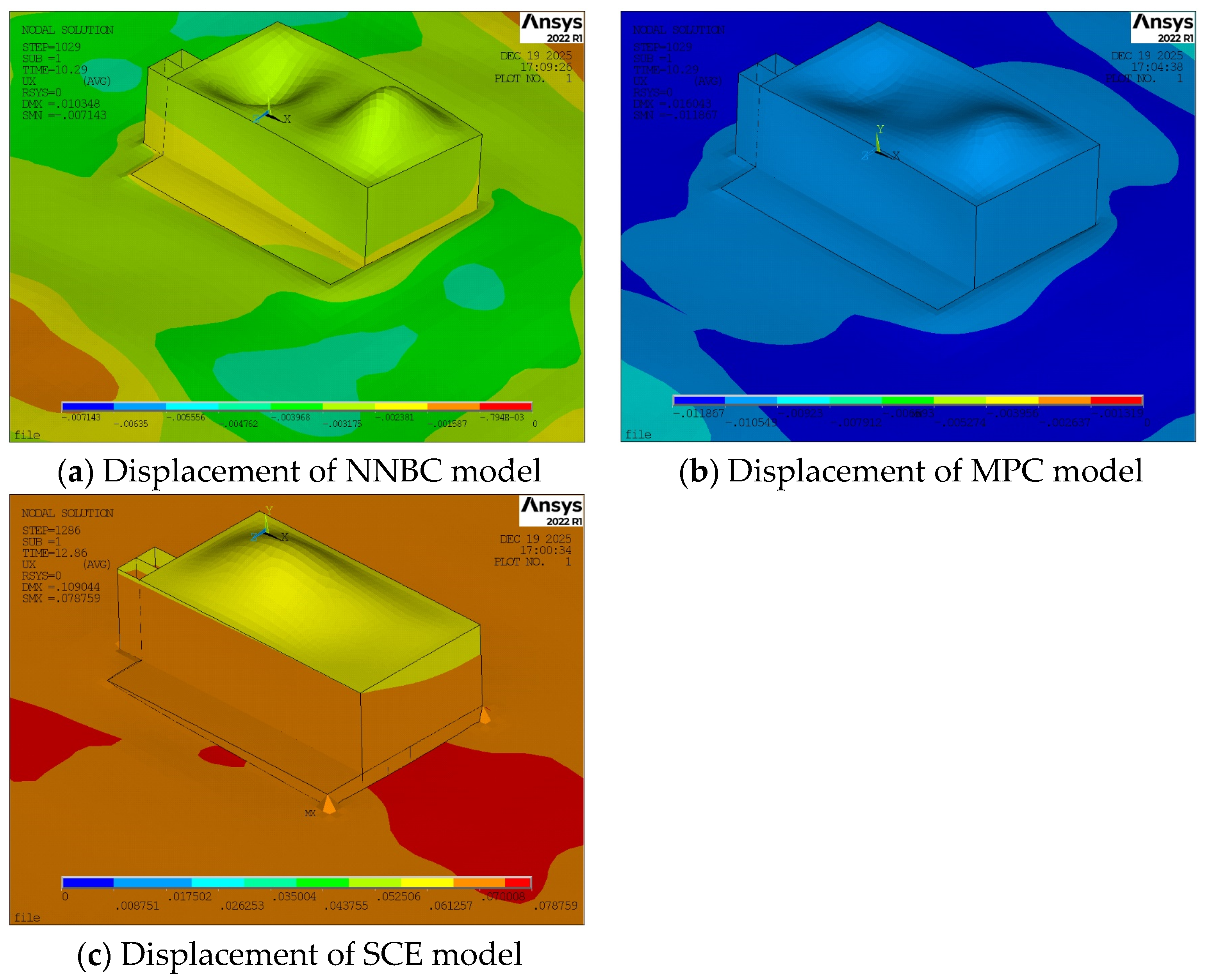
This paper primarily focuses on the analysis of the horizontal seismic response. Since the vibration characteristics in the two horizontal directions are essentially consistent, the vibration response along the long-side direction of the structure is selected for investigation. The displacement of each model is shown in Figure 10.

Figure 10. Displacement of each model.

5.1. Response of the Ground

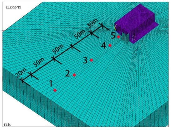
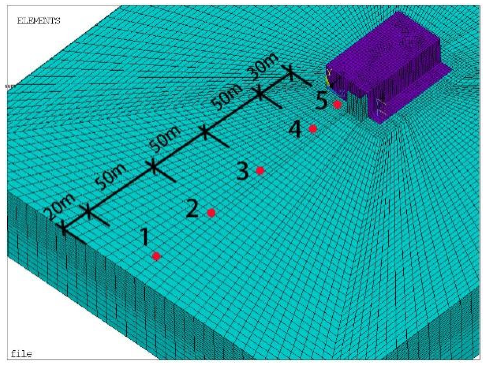
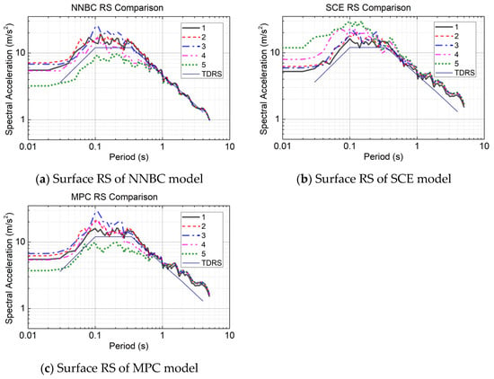
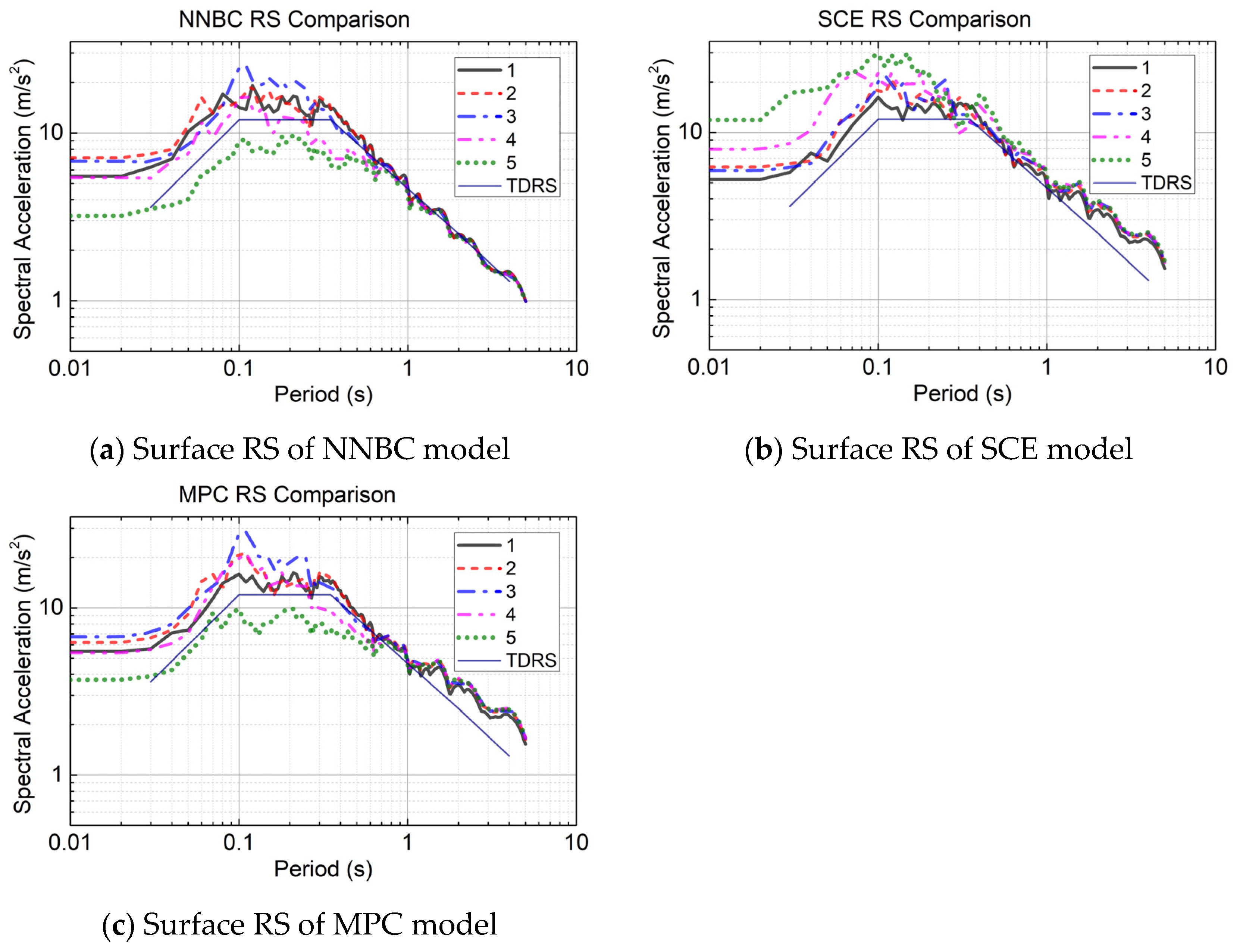
First, the ground surface response results from the three soil–structure contact models (NNBC, SCE, MPC) are analyzed. Five response points on the ground surface, ranging from near the boundary to close to the structure, were selected, as detailed in Figure 11. The RS results for the three models are shown in Figure 12. It is noted that at very short periods (T approaching zero) all response-spectrum curves flatten to a plateau: this is the expected asymptotic behavior, because the pseudo-spectral acceleration tends to the peak ground acceleration of the corresponding point as the period approaches zero, so the flat short-period values reflect the local peak ground acceleration rather than a numerical artefact.

Figure 11. Surface measurement point layout diagram.

Figure 12. Surface RS of various models.

Figure 11 defines the five surface monitoring points, from near the lateral boundary to adjacent to the structure; the response spectra at these points for the three interface models are compared in Figure 12 and interpreted below in terms of wave reflection and radiation at the soil–structure interface.

From the surface RS results of the NNBC model, it can be observed that Point 5, located closest to the structure, exhibits the smallest response spectrum amplitude. This is attributed to the relatively high stiffness of the structure, resulting in a smaller vibrational response. The NNBC causes the soil near the structure to be influenced by the structural behavior, thereby reducing the response spectrum amplitude in its vicinity. Point 3, situated near the middle of the soil domain, shows the largest response spectrum amplitude. This amplification is likely due to the superposition of waves reflected from the structure with the incoming seismic motion. Figure 12 also shows that the RS curve at Point 1, near the boundary, closely matches the TDRS. This demonstrates the effectiveness of the seismic input method and indicates that the viscoelastic boundary of the model effectively absorbs reflected waves. The RS curves for Points 2 and 4 fall between those of Points 1 and 3 as well as Points 5 and 3, respectively, which is reasonable. Furthermore, for periods greater than 0.6 s, the response spectrum curves from all points converge and essentially coincide with the TDRS.

The surface RS results from the SCE model indicate that Point 5, adjacent to the structure, has the largest RS amplitude. The amplitude at Point 4 is smaller than at Point 5. Points 2 and 3 show similar amplitudes, which are lower than Point 4. Point 1 exhibits the smallest amplitude, and its curve closely aligns with the TDRS. This suggests that in the SCE model, the ability of the structure and soil to separate during vibration means the structure does not restrain the surrounding soil’s response. Instead, vibrations reflected from the structure superimpose onto the adjacent soil, amplifying its response. The surface response then gradually diminishes from the structure towards the boundary. The close match of Point 1’s RS curve with the TDRS again validates the seismic input method and the viscoelastic boundary’s performance. Additionally, for periods greater than 0.6 s, the response spectra from all points converge. However, for periods exceeding 1 s, the RS curves exceed the TDRS.

The surface RS results of the MPC model show a distribution in the short-period range (periods < 0.6 s) similar to the NNBC model. Specifically, Point 5 near the structure has the smallest amplitude, Point 3 in the central area has the largest amplitude, Points 2 and 4 show intermediate values, and Point 1’s curve matches the TDRS well. This indicates that the MPC connection behaves similarly to the NNBC model in this range, with the structure restraining the vibration of the surrounding soil. However, in the long-period range (periods > 0.6 s), the RS curve resemble those of the SCE model. The RS curves from all points largely converge, and for periods greater than 1 s, they exceed the TDRS.

5.2. Response of the Structure

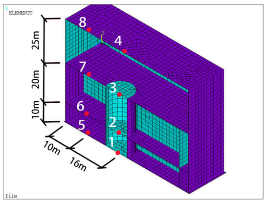
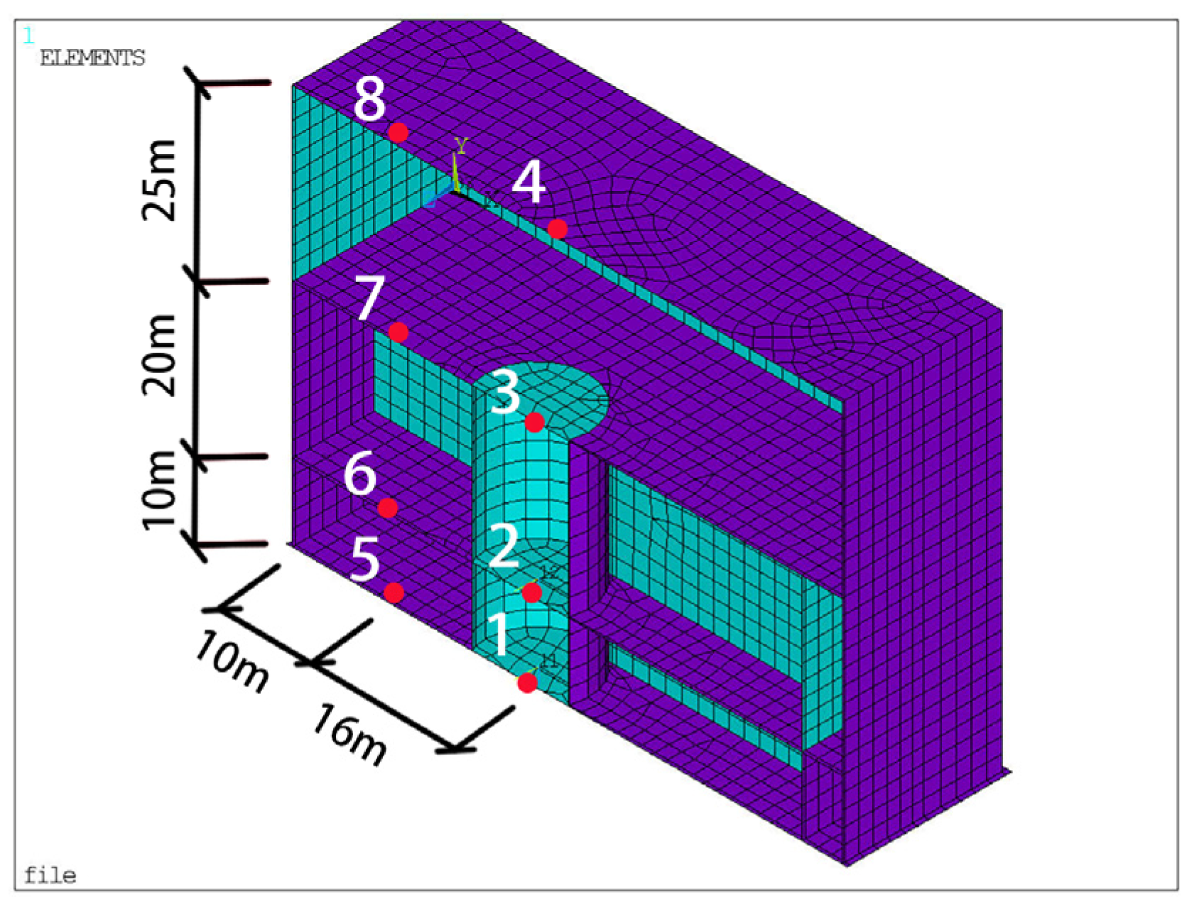
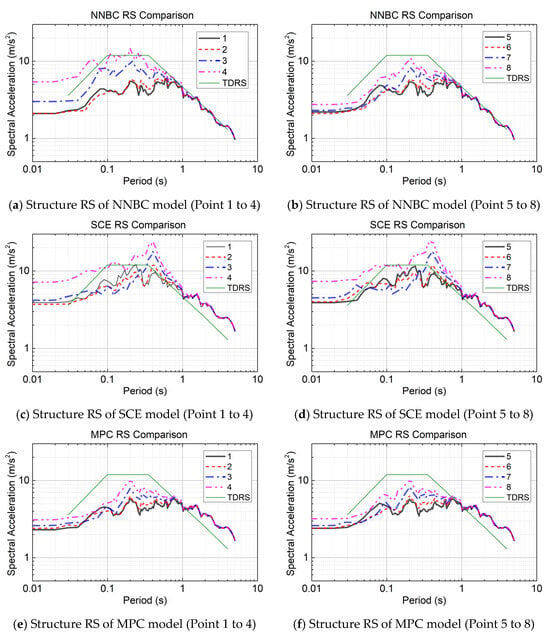
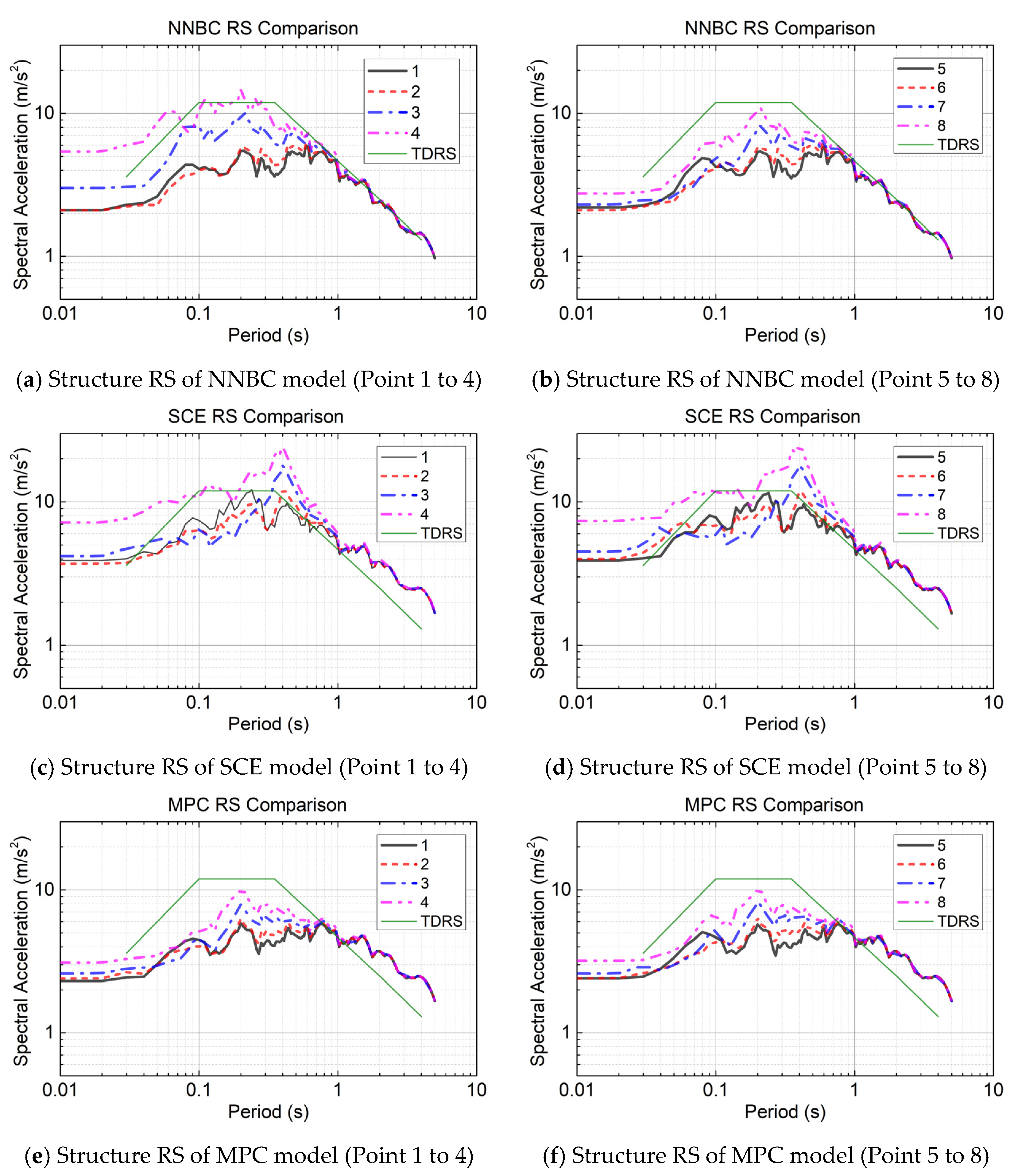
To investigate the horizontal vibrational response within the structure, this study selected three points inside the circular reactor cavity, corresponding to the second underground level, the first underground level, and the ground level, respectively. An additional point (Point 4) was selected on the corresponding floor slab. Furthermore, to mitigate the influence of the high stiffness of the circular cavity, Points 5 to 8 were chosen at typical locations within the nuclear island building; their specific positions are detailed in Figure 13. The vibrational response spectrum results at these points are shown in Figure 14.

Figure 13. Internal structure measurement point layout diagram.

Figure 14. Structure RS of various models.

Figure 13 shows the locations of the eight in-structure monitoring points (Points 1–8) at the second underground, first underground, ground and above-ground levels; the corresponding response spectra for the three interface models are compared in Figure 14 and discussed below.

The RS curves generally exhibit the characteristic of increasing amplitude from the second underground level to the second above-ground level. This trend aligns with the decreasing input seismic load from the model base to the ground surface and is consistent with the expected amplification of seismic response in above-ground structures with increasing height. It is noteworthy that all models show very close response spectrum curves between the points on the second and first underground levels. This is likely attributable to the relatively lower story height of the second underground level (9 m versus 18 m for the first underground level), resulting in higher stiffness and consequently similar vibrational responses in this region.

In the NNBC model, the RS curves for all measurement points on the structure converge for periods greater than 0.6 s and essentially coincide with the TDRS. In both the SCE and MPC models, the response spectra from various points also converge for periods beyond 0.6 s; however, for periods greater than 1 s, the RS curves exceed the TDRS. This indicates that the characteristics of the vibrational response spectra on the structure are fundamentally consistent with those observed on the ground surface near the structure across the three models.

The differences and commonalities among the models are analyzed below. The structural vibrational response of the SCE model is higher than that of the NNBC and MPC models. In both the SCE and MPC models, the response spectra at points inside and outside the reactor cavity are essentially identical. Conversely, in the NNBC model, differences exist in the response spectra between corresponding points on the first and second above-ground floors located inside and outside the cavity, with the points inside the cavity exhibiting larger amplitudes. For periods ranging from 0.1 s to 1 s, the RS amplitudes in both the NNBC and MPC models are generally lower than the surface TDRS. In the SCE model, the RS at the first above-ground level is close to the surface TDRS, while that at the second above-ground level exceeds it. Comparing the response spectrum curves of the three models reveals that the curves for the NNBC and MPC models are quite similar, with their peaks occurring around a period of 0.1 s. For the SCE model, however, the peak of the response spectrum curve shifts to a period of approximately 0.3 s.

5.3. Comparison of Response of the Interface on SCE Model

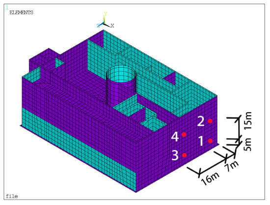
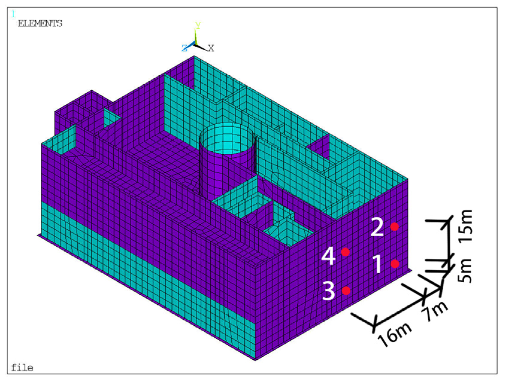
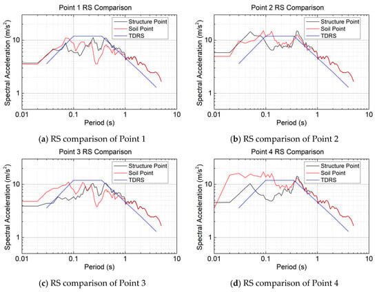
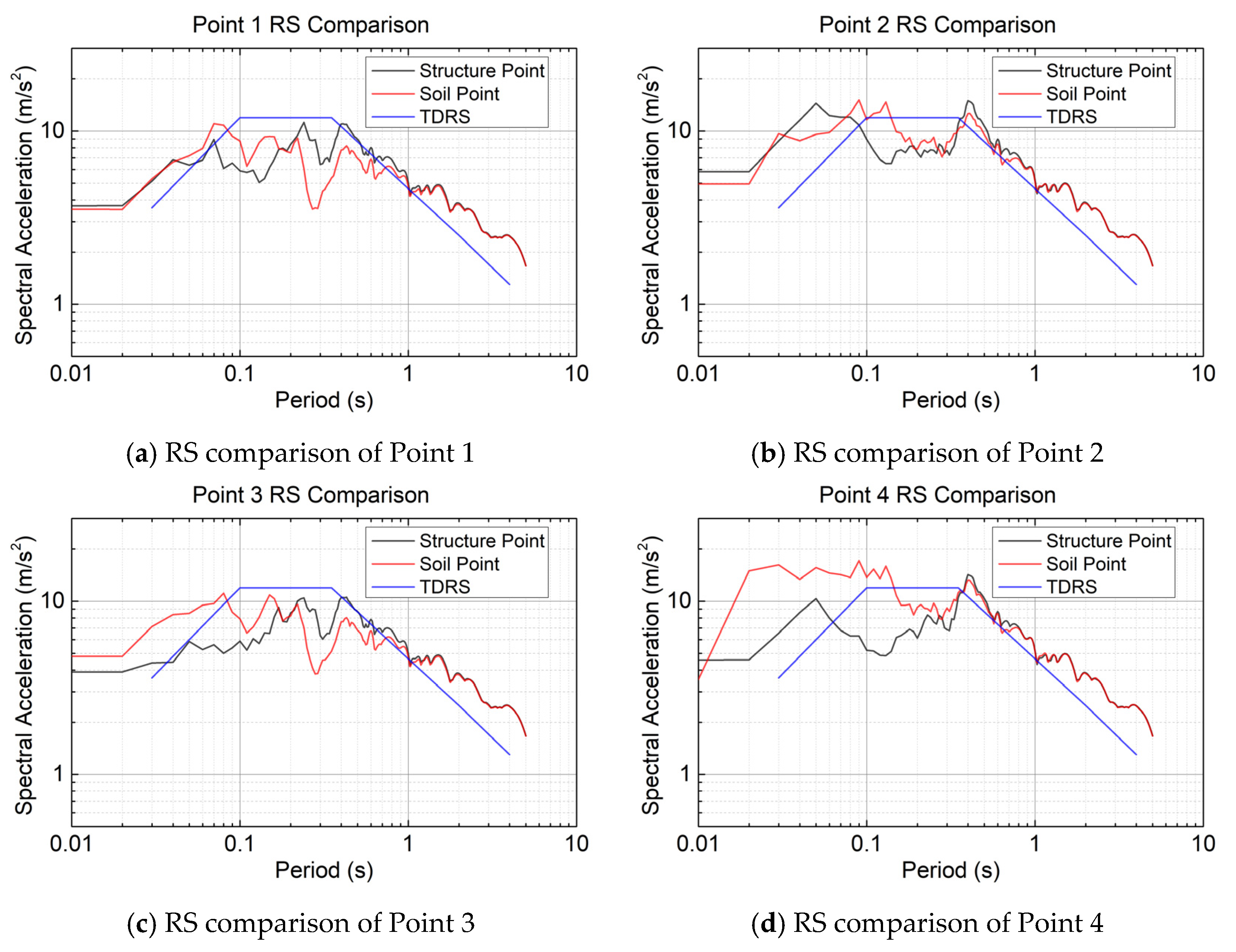
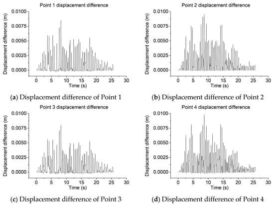
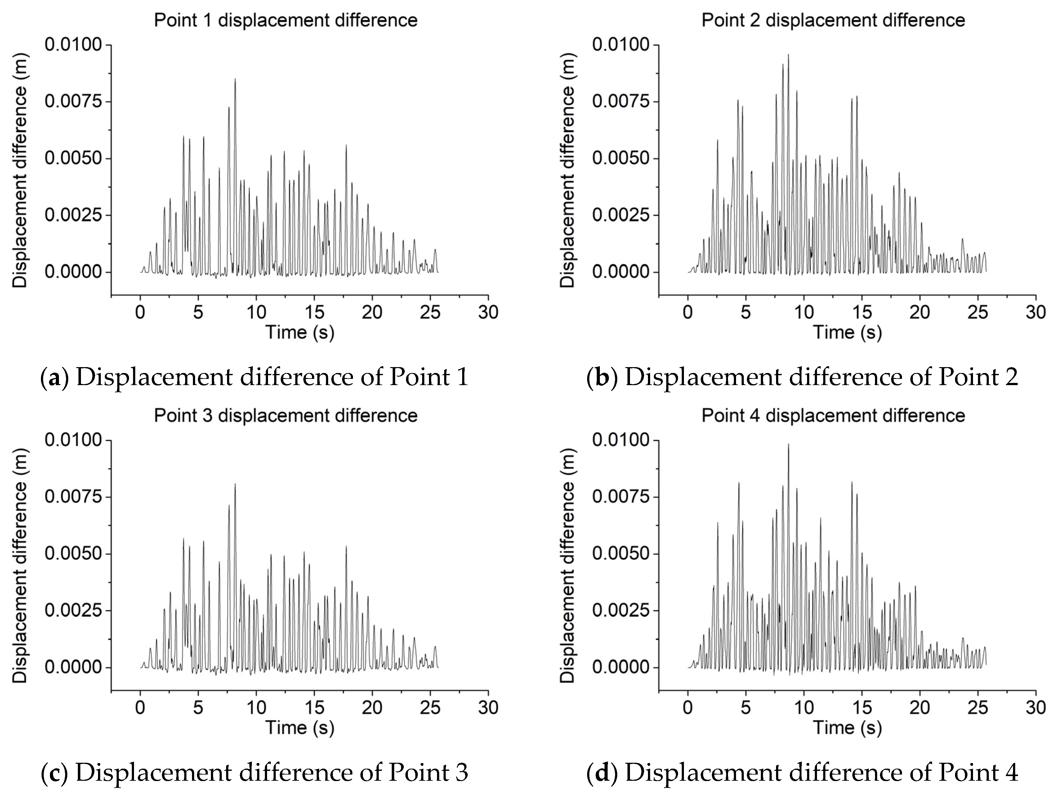
To investigate the differences between structural points and soil points in the SCE model, this study examined eight points (four pairs) located along the side of the structure in the short-side direction. To analyze the influence of burial depth and the presence of shear walls on the behavior of the contact elements, the four selected locations corresponded to the second underground level without a shear wall, the first underground level without a shear wall, the second underground level with a shear wall, and the first underground level with a shear wall. Each location contains one structural point and one adjacent soil point. The specific positions are detailed in Figure 15. The vibrational response spectrum results for these points are shown in Figure 16. The x-direction (horizontal, perpendicular to the wall face) displacement difference between the soil and structure points at each location is presented in Figure 17.

Figure 15. SCE model measurement point layout diagram.

Figure 16. Vibrational response spectrum results.

Figure 17. X-direction (perpendicular to the wall face) displacement difference of Points 1–4.

A comparison of the acceleration response spectra between the structural and soil points at the same location reveals significant differences in the period range less than 1.0 s, whereas the spectra essentially overlap for periods greater than 1.0 s. No clear, consistent pattern was identified within the range where differences occur. The displacement differential results indicate that the soil displacement consistently exceeds the structural displacement throughout the vibration process. The distribution of the displacement differential is generally consistent at the same burial depth. The peak displacement differential values for Points 1 to 4 are 0.85 cm, 0.96 cm, 0.81 cm, and 0.98 cm, respectively. This suggests that the magnitude of the displacement differential tends to increase with decreasing burial depth. The presence or absence of a shear wall appears to have a minor influence on the displacement differential.

The SCE interface uses a Coulomb friction model with a tangential friction coefficient mu = 0.4, a static-to-dynamic friction ratio of 1.25 and a decay coefficient of 0.8; the initial gap is zero and the soil and structure are initially in contact. The value mu = 0.4 is representative of soil–concrete interface friction reported in the literature [35,36,37]. The peak soil–structure relative (differential) displacement in the horizontal x-direction, i.e., perpendicular to the wall face, remains below 1.0 cm (0.81–0.98 cm, Figure 17); because the normal contact gap was not evaluated directly, this relative displacement is interpreted as indicating limited relative slippage and deformation across the interface rather than as direct evidence of negligible contact opening. A parametric study of the friction coefficient is recommended to bound the response.

From the perspective of different depths, the overall RS amplitudes at Point 2 (first underground level) are higher than those at Point 1 (second underground level), and similarly, Point 4 shows higher amplitudes than Point 2. This trend corresponds to the distribution pattern of the input motion amplitudes with depth. Regarding the effect of the shear wall, a comparison between Points 1 (without wall) and 3 (with wall) shows that the RS curves of the structural points are quite similar. For the soil points, the RS at Point 3 exceeds that at Point 1 for periods less than 0.9 s, while the spectra are relatively close for other periods. Similarly, comparing Points 2 (without wall) and 4 (with wall) reveals closely matched RS on the structure. For the soil points at these locations, the RS at Point 4 is higher than that at Point 2 for periods less than 0.9 s, with the curves being similar elsewhere.

6. Discussion and Limitations

6.1. Discussion

Modal analyses give fundamental frequencies of 1.383 Hz (NNBC), 1.159 Hz (SCE) and 1.160 Hz (MPC). The separable and constraint interfaces therefore soften the coupled soil–structure system and lengthen its fundamental period relative to the fully bonded case. This period lengthening is consistent with the response-spectra results of Section 5, in which the SCE and MPC models show enhanced long-period (T > 1 s) ordinates together with a reduced in-structure short-period demand, and it is consistent with the interpretation that the interface-modeling assumption, rather than the soil profile alone, controls how the seismic demand is distributed between the ground and the structure. The modal frequencies and the spectral ordinates above are the observed numerical results; the attribution of the peak shift from about 0.1 s to about 0.3 s and of the long-period amplification to interface decoupling is a plausible physical interpretation supported by, but not conclusively demonstrated by, these results.

Table 2 quantifies these interface-modeling effects. At the ground surface, the two non-bonded interfaces act in the same direction but with very different intensity: relative to the NNBC model (mean 18.1, maximum 25.0 m/s²), the SCE interface raises the peak PSA to 22.3 and 30.0 m/s² (ratios of 1.23 and 1.20), whereas the MPC interface gives only 19.4 and 28.4 m/s² (1.07 and 1.14). Inside the structure, the contrast is larger and the ordering changes: SCE almost doubles the mean in-structure peak PSA (from 8.6 to 16.5 m/s², ratio 1.93) and raises the maximum from 14.6 to 25.0 m/s² (1.71), while MPC keeps the mean at 7.6 m/s² (0.89) and reduces the maximum to 10.3 m/s² (0.71). The same pattern appears in the peak floor acceleration (the T -> 0 ordinate, i.e., the peak acceleration response), which increases from 5.40 m/s² (NNBC) to 7.35 m/s² (SCE, 1.36) but drops to 3.20 m/s² (MPC, 0.59). Allowing the interface to separate and slide therefore concentrates additional demand both at the ground surface and, more strongly, within the structure, whereas the constraint interface transmits the least demand of the three and gives the lowest in-structure and floor accelerations. Since the peak soil–structure relative displacement in the x-direction remains small (0.81–0.98 cm for SCE, and bonded for NNBC and MPC) and the normal contact gap was not evaluated, these differences are interpreted as being governed by the interface stiffness and frictional coupling rather than by gross separation, which is consistent with the period lengthening identified from the modal analyses.

Table 2. Quantification of the interface-modeling effects on ground and structural response.

Quantity	NNBC	SCE	MPC	SCE/NNBC	MPC/NNBC
Mean ground-surface peak PSA (m/s2)	18.1	22.3	19.4	1.23	1.07
Max ground-surface peak PSA (m/s2)	25.0	30.0	28.4	1.20	1.14
Mean in-structure peak PSA (m/s2)	8.6	16.5	7.6	1.93	0.89
Max in-structure peak PSA (m/s2)	14.6	25.0	10.3	1.71	0.71
Max peak floor acceleration, T -> 0 (m/s2)	5.40	7.35	3.20	1.36	0.59
Peak soil–structure relative displacement (cm)	bonded	0.81–0.98	bonded	-	-

6.2. Limitations

First, the soil is represented by an equivalent-linear model whose strain-compatible modulus reduction and hysteretic (Rayleigh) damping are fitted at the site fundamental frequency and the dominant input frequency (Section 3.2). Such a model cannot reproduce cumulative plastic deformation or pore-pressure generation, and it applies the correct damping only at the fitted frequencies. Near a stiff embedded structure, the local strains can exceed the range over which these equivalent parameters are representative, so the short-period in-structure ordinates reported for the SCE model in Table 2 carry greater uncertainty than the long-period ground ordinates.

Second, the spatial discretization and domain size are adequate but bounded. In the softest layer (strain-compatible Vs = 226 m/s, Table 1), the 1.0 m element resolves the shortest shear wavelength of interest to about 6.8 m at 33 Hz, i.e., about seven elements per wavelength, so the one-eighth-wavelength criterion [29] is satisfied up to about 28 Hz and is marginally relaxed at 33 Hz; the lateral boundaries lie 207.5 m and 152.5 m from the structure edges, exceeding three times the structural plan dimensions required by GB 50267-2019 [30]. Input motion containing significant energy above about 28 Hz would require a correspondingly finer mesh. No alternative mesh densities or computational domain sizes were analyzed, so the model is not claimed to be mesh-converged; the wavelength criterion and the agreement with EERA verify the free-field response only, not the coupled soil–structure model, and local stress and displacement gradients near the soil–structure interface may require a finer discretization.

Third, the results derive from a single horizontal component of one artificial accelerogram compatible with the 1%-in-100-years design spectrum and from a linear–elastic structural model (Section 3.1 and Section 4.1). Multiple recorded motions, the vertical component, and inelastic structural behavior would change the quantitative ratios in Table 2; the qualitative ranking of the three interface models is expected to remain robust, but the magnitudes should be re-checked for other inputs.

Fourth, the SCE interface adopts a single tangential friction coefficient (mu = 0.4), a mid-range value supported by soil-concrete interface friction data [35,36,37]. This coefficient governs the tangential load transfer between the soil and the structure: as mu increases, the interface approaches the fully bonded (NNBC) limit, whereas as mu tends to zero, it approaches frictionless sliding and the two media decouple, so mu directly controls the SCE/NNBC ratios reported in Table 2. Because a single mid-range value is adopted here, a parametric study over mu is recommended to bound the response.

7. Conclusions

This study established a 3D finite element model based on a new-type buried NPP structure to compare the differences among three soil–structure connection methods: NNBC, SCE, and MPC. Utilizing site-specific seismic response characteristics as input conditions and incorporating a viscoelastic artificial boundary, the model analyzed the seismic dynamic responses of both the soil and the structure under these different connection methods. Three key conclusions are drawn from this research.

• In the finite element models using the NNBC and MPC methods, the structure exerts a restraining effect on the seismic response of the surrounding soil. Conversely, in the model employing the SCE method, the structure produces an amplifying effect on the seismic response of the adjacent soil.
• The seismic response within the structure is significantly larger in the model utilizing the SCE method compared to the models using the NNBC or MPC methods.
• For the finite element model with the contact connection, the presence or absence of a shear wall has a minor influence on the acceleration RS and displacements of both the structure and the soil. Regarding the acceleration response spectra, notable differences exist between the soil and structure at the same location, but no clear, consistent pattern is observed. Concerning displacements, the soil displacement is consistently greater than the structural displacement throughout the seismic response.
• Quantitatively, the SCE model yields ground-surface peak spectral accelerations of 16.2–30.0 m/s² (mean 22.3 m/s²) versus 9.7–25.0 m/s² (mean 18.1 m/s²) for NNBC and 9.9–28.4 m/s² (mean 19.4 m/s²) for MPC, as well as in-structure peak responses up to 25.0 m/s² compared with 14.6 m/s² (NNBC) and 10.3 m/s² (MPC); the peak soil–structure relative displacement in the SCE model remains below 1.0 cm, indicating negligible interface opening.
• For design practice, and in line with ASCE 4-16 and GB 50267-2019, the SCE model produced higher seismic demands than the bonded representations under the investigated conditions (single structural configuration, single soil profile and single seismic input); a separable frictional contact interface is therefore advisable for bounding the soil amplification adjacent to the structure and the in-structure demand in similar cases, whereas bonded representations (NNBC, MPC) may under-estimate these demands. The broader applicability of this recommendation requires further verification.

References

- Witter, P.K.; Champine, B.; Tamashiro, A.S.; Maggi, P. A Review of the Lawrence Livermore Nuclear Accident Dosimeter 1980s-present. Radiat. Meas. 2024, 179, 107309. [Google Scholar] [CrossRef] [Scilit]
- Bararnia, M.; Hassani, N.; Ganjavi, B.; Ghodrati Amiri, G. Estimation of inelastic displacement ratios for soil-structure systems with embedded foundation considering kinematic and inertial interaction effects. Eng. Struct. 2018, 159, 252–264. [Google Scholar] [CrossRef] [Scilit]
- Mirzaie, F.; Mahsuli, M.; Ghannad, M.A. Probabilistic analysis of soil-structure interaction effects on the seismic performance of structures. Earthq. Eng. Struct. Dyn. 2017, 46, 641–660. [Google Scholar] [CrossRef] [Scilit]
- Renzi, S.; Madiai, C.; Vannucchi, G. A simplified empirical method for assessing seismic soil-structure interaction effects on ordinary shear-type buildings. Soil Dyn. Earthq. Eng. 2013, 55, 100–107. [Google Scholar] [CrossRef] [Scilit]
- Mylonakis, G.; Gazetas, G. Seismic soil-structure interaction: Beneficial or detrimental? J. Earthq. Eng. 2000, 4, 277–301. [Google Scholar] [CrossRef] [Scilit]
- Isik, E.; Avcil, F.; Buyuksarac, A.; Arkan, E.; Harirchian, E. Impact of local soil conditions on the seismic performance of reinforced concrete structures: In the context of the 2023 Kahramanmaraş earthquakes. Appl. Sci. 2025, 15, 2389. [Google Scholar] [CrossRef] [Scilit]
- Tuñón-Sanjur, L.; Orr, R.S.; Tinic, S.; Ruiz, D.P. Finite element modeling of the AP1000 nuclear island for seismic analyses at generic soil and rock sites. Nucl. Eng. Des. 2007, 237, 1474–1485. [Google Scholar] [CrossRef] [Scilit]
- Saxena, N.; Paul, D.K.; Kumar, R. Effects of slip and separation on seismic SSI response of nuclear reactor building. Nucl. Eng. Des. 2011, 241, 12–17. [Google Scholar] [CrossRef] [Scilit]
- Saxena, N.; Paul, D.K. Effects of embedment including slip and separation on seismic SSI response of a nuclear reactor building. Nucl. Eng. Des. 2012, 247, 23–33. [Google Scholar] [CrossRef] [Scilit]
- Bolisetti, C.; Whittaker, A.S. Site Response, Soil-Structure Interaction and Structure-Soil-Structure Interaction for Performance Assessment of Buildings and Nuclear Structures; Technical Report MCEER-150002; State University of New York at Buffalo: Buffalo, NY, USA, 2015. [Google Scholar]
- Naserkhaki, S.; Pourmohammad, H. SSI AND SSSI EFFECTS IN SEISMIC ANALYSIS OF TWIN BUILDINGS: Discrete model concept. J. Civ. Eng. Manag. 2012, 18, 890–898. [Google Scholar] [CrossRef] [Scilit]
- Farahani, R.V.; Dessalegn, T.M.; Vaidya, N.R.; Bazan-Zurita, E. Seismic soil-structure interaction analysis of a nuclear power plant building founded on soil and in degraded concrete stiffness condition. Nucl. Eng. Des. 2016, 297, 320–326. [Google Scholar] [CrossRef] [Scilit]
- Wang, G.; Yuan, M.; Ma, X.; Wu, J. Numerical study on the seismic response of the underground subway station- surrounding soil mass-ground adjacent building system. Front Struct. Civ. Eng. 2017, 11, 424–435. [Google Scholar] [CrossRef] [Scilit]
- de Borbón, F.; Domizio, M.; Ambrosini, D.; Curadelli, O. Influence of various parameters in the seismic soil-structure interaction response of a nuclear power plant. Eng. Struct. 2020, 217, 110820. [Google Scholar] [CrossRef] [Scilit]
- Abell, J.A.; Orbović, N.; McCallen, D.B.; Jeremic, B. Earthquake soil-structure interaction of nuclear power plants, differences in response to 3-D, 3 × 1-D, and 1-D excitations. Earthq. Eng. Struct. Dyn. 2018, 47, 1478–1495. [Google Scholar] [CrossRef] [Scilit]
- Ba, Z.; Fu, J.; Zhu, Z.; Zhong, H. An end-to-end 3d seismic simulation of underground structures due to point dislocation source by using an FK-FEM hybrid approach. Front. Struct. Civ. Eng. 2022, 16, 1515–1529. [Google Scholar] [CrossRef] [Scilit]
- Li, L.; Chen, Q.; Pan, R. Analysis of the Influence of Structure–Soil–Structure Interaction on the Seismic Response for Nuclear Power Plant ASTS. Energies 2023, 16, 194. [Google Scholar] [CrossRef] [Scilit]
- Hu, Y.; Khatiwada, P.; Tsang, H.H.; Menegon, S. Site-specific response spectra and accelerograms on bedrock and soil surface. CivilEng 2023, 4, 311–332. [Google Scholar] [CrossRef] [Scilit]
- Lv, H.; Chen, S.L. Analysis of nonlinear soil-structure interaction using partitioned method. Soil Dyn. Earthq. Eng. 2022, 162, 107470. [Google Scholar] [CrossRef] [Scilit]
- Shahraki, M.; Tessari, A.; Bolisetti, C.; Kurt, E.; Kim, K. Experimental study on sliding at the soil-structure interface of a shallow foundation. Geotech. Test. J. 2024, 47, 521–538. [Google Scholar] [CrossRef] [Scilit]
- Huo, H.; Bobet, A.; Fernández, G.; Ramírez, J. Load Transfer Mechanisms between Underground Structure and Surrounding Ground: Evaluation of the Failure of the Daikai Station. J. Geotech. Geoenviron. Eng. 2005, 131, 1522–1533. [Google Scholar] [CrossRef] [Scilit]
- Farghaly, A.A.; Ahmed, H.H. Contribution of Soil-Structure Interaction to Seismic Response of Buildings. KSCE J. Civ. Eng. 2013, 17, 959–971. [Google Scholar] [CrossRef] [Scilit]
- Liu, Y.; Chen, Q.; Chen, X.; Liao, C. Seismic Damage Mechanism of Five-Story and Three-Span Underground Complex in Soft Soil Site. Buildings 2025, 15, 2380. [Google Scholar] [CrossRef] [Scilit]
- Hui, B.; Yan, G.; Xu, C. Influence of Different Soil-Structure Interface Model on Seismic Response of Structure in the Liquefaction Interlayer Site. Technol. Earthq. Disaster Prev. 2025, 20, 127–139. (In Chinese) [Google Scholar]
- Liu, S.; Li, P.; Zhang, W.; Lu, Z. Experimental study and numerical simulation on dynamic soil-structure interaction under earthquake excitations. Soil Dyn. Earthq. Eng. 2020, 138, 106333. [Google Scholar] [CrossRef] [Scilit]
- Dou, P.; Liu, H.; Xu, C.; Wang, J.; Sun, Y.; Du, X. Numerical analysis on seismic response and failure mechanism of articulated pile–structure system in a liquefiable site from shaking-table experiments. Front Struct. Civ. Eng. 2024, 18, 1117–1133. [Google Scholar] [CrossRef] [Scilit]
- Onitsuka, S.; Iijima, T.; Yamada, T.; Yoshimura, S. Seismic analysis of nuclear power plants by using three-dimensional finite element models: A review. J. Nucl. Sci. Technol. 2019, 56, 1–16. [Google Scholar] [CrossRef] [Scilit]
- Amorosi, A.; Boldini, D.; di Lernia, A. Dynamic soil-structure interaction: A three-dimensional numerical approach and its application to the Lotung case study. Comput. Geotech. 2017, 90, 34–54. [Google Scholar] [CrossRef] [Scilit]
- Kuhlemeyer, R.L.; Lysmer, J. Finite element method accuracy for wave propagation problems. J. Soil Mech. Found. Div. 1973, 99, 421–427. [Google Scholar] [CrossRef] [Scilit]
- GB 50267-2019; Standard for Seismic Design of Nuclear Power Plants. China Planning Press: Beijing, China, 2019.
- Du, X.L.; Xu, Z.G.; Xu, C.S.; Li, Y.; Jiang, J.W. Time-history analysis method for soil-underground structure system based on equivalent linear method. Chin. J. Geotech. Eng. 2018, 40, 2155–2163. [Google Scholar] [CrossRef]
- Liu, J.; Du, Y.; Du, X.; Wang, Z.; Wu, J. 3D viscous-spring artificial boundary in time domain. Earthq. Eng. Eng. Vib. 2006, 5, 93–102. [Google Scholar] [CrossRef] [Scilit]
- Gu, Y.; Liu, J.B.; Du, Y.X. 3D consistent viscous-spring artificial boundary and viscous-spring boundary element. Eng. Mech. 2007, 24, 31–37. [Google Scholar]
- Jingbo, L.; Yandong, L. A direct method for analysis of dynamic soil-structure interaction. China Civ. Eng. J. 1998, 31, 55–64. [Google Scholar]
- Potyondy, J.G. Skin friction between various soils and construction materials. Geotechnique 1961, 11, 339–353. [Google Scholar] [CrossRef] [Scilit]
- Lu, D.C.; Wang, X.; Luo, L.; Du, X.L. Research on the seismic responses of underground structures considering the soil and structure contact. J. Disaster Prev. Mitig. Eng. 2017, 37, 177–186. [Google Scholar]
- Peng, Y.; Liu, B.; Wang, G.; Wang, Q. Analyses of the suction anchor-sandy soil interactions under slidable pulling action using DEM-FEM coupling method: The interface friction effect. J. Mar. Sci. Eng. 2024, 12, 535. [Google Scholar] [CrossRef] [Scilit]
Disclaimer/Publisher’s Note: The statements, opinions and data contained in all publications are solely those of the individual author(s) and contributor(s) and not of MDPI and/or the editor(s). MDPI and/or the editor(s) disclaim responsibility for any injury to people or property resulting from any ideas, methods, instructions or products referred to in the content. |
© 2026 by the authors. Licensee MDPI, Basel, Switzerland. This article is an open access article distributed under the terms and conditions of the Creative Commons Attribution (CC BY) license.