


Abstract
High levels of photovoltaic (PV) generation in distribution networks create substantial uncertainty and voltage variability, which limits the effectiveness of conventional deterministic distribution network reconfiguration (DNR) strategies. In PV-dominated feeders, rare but severe operating conditions may considerably influence active power losses and voltage stability. To address this challenge, this paper proposes a risk-informed optimization framework for DNR that combines reinforcement learning with probabilistic performance assessment. A Deep Q-Network (DQN) agent is designed to support the selection of feasible radial switching configurations by interacting with the distribution network environment. Throughout the learning process, candidate network topologies are evaluated through radial load flow calculations, while a composite objective function incorporating active power losses and voltage deviation steers the agent toward improved configurations. The training stage is based on deterministic performance indices; however, the final reconfiguration solution is assessed under uncertainty to examine its operational robustness. For this purpose, extensive Monte Carlo simulations are performed to capture the stochastic behavior of PV generation and load demand. Tail-based risk metrics, including Value at Risk (VaR) and Conditional Value at Risk (CVaR), are computed for both loss and voltage deviation indices, providing insight into the performance of the selected configuration under unfavorable operating scenarios. The proposed framework is first validated on the IEEE 33-bus distribution system and then further investigated on the IEEE 69-bus network. The obtained results demonstrate that the proposed DQN-based reconfiguration approach can enhance voltage profiles and reduce power losses under high PV penetration. In addition, the probabilistic analysis identifies meaningful trade-offs between efficiency and voltage robustness, highlighting the importance of considering uncertainty-driven risk assessment in computational decision-making for modern active distribution networks.
1. Introduction
1.1. Motivation
The growing integration of photovoltaic (PV) generation at the distribution level has introduced increased variability into feeder operation. In radial networks originally designed for largely unidirectional power transfer, fluctuations in local generation can lead to rapid changes in voltage magnitude and power flow patterns, particularly during transitions in irradiance or demand [1]. Consequently, operating conditions that were previously managed under relatively stable assumptions now require more adaptive control strategies. Distribution system operators must ensure acceptable loss levels and voltage profiles despite short-term variations that may not be well represented by nominal operating points.
Among available operational measures, distribution network reconfiguration (DNR) provides a flexible mechanism for adjusting network topology without major infrastructure upgrades. By altering switch statuses while preserving radiality, operators can influence power flow paths and voltage distribution across the feeder. However, the effectiveness of a given switching configuration depends strongly on the prevailing load and generation conditions [2,3]. A topology that reduces losses during high PV output may produce less favorable voltage behavior under reduced generation or peak demand [4]. As the number of feasible switching combinations increases, systematically evaluating all configurations under multiple operating states becomes computationally demanding. Moreover, assessing performance solely on the basis of expected or average conditions may overlook operating states that occur infrequently but have significant technical impact. This operational context motivates decision-making approaches that can account for variability while maintaining computational practicality, particularly in distribution networks with substantial PV penetration.
1.2. Literature Review
Distribution network reconfiguration (DNR) has been extensively investigated as an effective operational strategy for improving the performance of distribution feeders. By modifying the network topology through switching operations, DNR can reduce active power losses, improve voltage profiles, and enhance the operational flexibility of distribution systems. However, the increasing penetration of renewable energy resources, particularly photovoltaic (PV) generation, has introduced new challenges to conventional reconfiguration approaches. The optimality of a switching configuration is no longer determined only by network topology but also depends on the interaction between variable generation patterns and changing load conditions.
Several studies have explored topology-based control strategies to mitigate voltage fluctuations in PV-rich distribution networks while reducing the dependence on additional power-electronic regulation devices [5]. Alongside these efforts, DNR has frequently been formulated as a multi-objective optimization problem, where loss reduction, voltage improvement, and reliability-related objectives are considered simultaneously. For example, epsilon-constrained optimization combined with fuzzy satisfaction approaches has been applied to minimize active power losses while improving reliability indicators such as energy not served (ENS) [6].
The increasing uncertainty associated with distributed generation (DG) output and load demand has gradually shifted research attention from deterministic formulations toward uncertainty-aware approaches. Scenario-based and iterative optimization frameworks have been developed to evaluate whether reconfiguration decisions remain effective under different operating conditions. In this context, metaheuristic-based methods evaluated on benchmark systems, including IEEE 33-bus, 85-bus, and larger synthetic feeders, have demonstrated the importance of considering DG and load variability during the optimization process [7]. Beyond standalone reconfiguration, some studies have investigated coordination with other flexible resources. For instance, two-stage frameworks have been proposed in which EV charging management is optimized before performing network reconfiguration, allowing the interaction between transportation flexibility and distribution system operation to be considered [8]. Similar integrated approaches have also been explored in energy systems involving flexible building operation, where network constraints and equipment limitations are simultaneously considered [9].
A considerable portion of previous DNR research has relied on heuristic, metaheuristic, and mathematical optimization techniques. Harmony Search-based methods have been employed to improve voltage security indices and reduce feeder losses; however, their validation has often been limited to specific benchmark networks [10]. Other evolutionary algorithms, such as bacterial foraging, cuckoo search, and gravitational search algorithms, have also been applied to discrete switching problems with the primary goals of reducing losses and improving voltage quality [11,12,13]. Although these methods have achieved promising results, their performance is generally influenced by algorithmic parameters, search mechanisms, and repeated optimization requirements when operating conditions change.
To provide more structured formulations, mathematical programming approaches have also been investigated for DNR problems. Mixed-integer second-order cone programming (MISOCP) has been applied to hourly reconfiguration problems considering stochastic DG and load variations, leading to reductions in daily energy losses [14]. Robust optimization frameworks have further been introduced to handle uncertainty by considering unfavorable operating conditions during the decision-making process [15]. In addition, some studies have extended the problem formulation by simultaneously optimizing DG placement, sizing, and network reconfiguration to address both operational and planning objectives [16]. Solver-based models, including CPLEX-based formulations, have also demonstrated the capability of mathematical optimization approaches for improving feeder performance under different operating scenarios [17]. Nevertheless, the computational burden of solving large-scale mixed-integer formulations remains an important consideration, particularly for systems requiring frequent operational decisions.
Recent research has also examined hybrid evolutionary methods that combine network reconfiguration with additional operational objectives. For example, GWO–PSO-based approaches have been developed for coordinated DG allocation and feeder reconfiguration with the aim of reducing power losses [18]. EMA–WGA frameworks have incorporated reliability indices, including AENS, SAIFI, and SAIDI, while improving network efficiency [19]. Other studies have integrated radiality-preserving evolutionary mechanisms with OpenDSS-based power-flow analysis to simultaneously optimize losses and voltage deviations [20,21]. Furthermore, modified binary PSO formulations have been proposed to improve the exploration capability of discrete switching spaces [22]. These studies demonstrate the continuous effort to improve the search capability of optimization-based DNR methods; however, most approaches still require solving an optimization problem for each operating condition.
More recently, reinforcement learning (RL) has attracted increasing attention for distribution network reconfiguration due to its capability of learning decision policies through interaction with the system environment. Unlike conventional optimization methods that repeatedly solve the optimization problem, RL-based approaches attempt to learn an operational policy that maps system conditions to appropriate switching decisions. Deep reinforcement learning methods, including DQN and NoisyNet-DQN variants, have been applied to reduce power losses and voltage deviations in distribution feeders [23,24]. Other studies have extended RL-based formulations by incorporating reliability-related factors, such as switch failure probabilities, into the decision process [25]. Comparative investigations of advanced DRL architectures, including dueling DQN, prioritized experience replay, soft actor–critic (SAC), and proximal policy optimization (PPO), have further explored the capability of learning-based methods in handling large discrete action spaces. To improve computational efficiency, action-space reduction and sampling strategies have also been proposed [26,27]. In addition, explainable RL approaches have recently been introduced to provide insight into how system states influence the switching decisions generated by trained agents [28].
Although these developments have significantly improved the capability of DNR methods, several research challenges remain unresolved. A large number of existing studies evaluate the performance of reconfiguration strategies using average indicators, such as expected power loss reduction or mean voltage deviation. Consequently, the behavior of the obtained solutions under rare but technically significant operating conditions is often not fully characterized. In particular, the combined impact of correlated load–PV uncertainty and the resulting tail behavior of operational indicators has received limited attention. Therefore, Table 1 compares representative DNR approaches and highlights the limited application of explicit risk measures, including Value at Risk (VaR) and Conditional Value at Risk (CVaR), for evaluating loss and voltage deviation under uncertain renewable generation conditions.
Table 1.
Comparison of recent DNR methods.
As summarized in Table 1, existing DNR studies, including metaheuristic methods [7,8,9,10,11,12,13,14,15,16,17,18,19,20,21,22], uncertainty-based optimization formulations [14,15,16,17], and DRL-based approaches [23,24,25,26,27,28], have mainly focused on improving conventional operational indicators, such as active power loss reduction and voltage profile enhancement. However, the evaluation of reconfiguration decisions under unfavorable but plausible operating conditions has received comparatively less attention. In particular, explicit quantification of tail behavior through risk measures such as VaR and CVaR, together with correlated modeling of load and PV generation uncertainties, remains limited in many existing studies. These limitations motivate the development of the proposed framework, which integrates DRL-based reconfiguration with uncertainty-aware operational risk assessment.
Although recent studies have significantly advanced DNR through stochastic optimization, risk assessment approaches, and DRL-based decision-making, an integrated framework that simultaneously addresses these aspects remains limited. Stochastic DNR studies mainly focus on representing uncertainty in load and renewable generation, while risk-oriented approaches often evaluate robustness through predefined optimization formulations. Meanwhile, recent DRL-based methods have demonstrated promising performance for reconfiguration problems but generally emphasize average operational improvements rather than explicit evaluation of uncertainty-driven tail behavior. Therefore, a research gap remains in developing a state-aware learning framework that combines probabilistic load–PV uncertainty modeling, tail-risk assessment, and adaptive reconfiguration decisions for PV-rich distribution networks.
1.3. Contributions
This study proposes a reinforcement learning-based framework for distribution network reconfiguration in PV-rich distribution systems considering operational uncertainty. Unlike conventional approaches that mainly optimize reconfiguration for a single operating condition, the proposed framework learns feasible switching decisions while considering variations in load demand and renewable generation. The main contributions of this work are summarized as follows:
It is worth emphasizing that the role of reinforcement learning in this study is not to replace classical optimization methods for small deterministic benchmark systems. Instead, RL is employed as a state-dependent decision-making mechanism capable of adapting switching decisions to different operating conditions. The IEEE 33-bus feeder is used as the primary validation system to evaluate the capability of the proposed method under diverse network states, while the IEEE 69-bus feeder is considered for additional validation.
- A state-aware DQN-based reconfiguration framework for PV-rich distribution networks. The proposed method employs a Deep Q-Network (DQN) agent to select feasible radial switching configurations through interaction with the distribution network environment. The learning process considers system states, including bus loads, PV-based DG injections, and voltage conditions, while experience replay and a target network are used to improve training stability.
- Probabilistic representation of renewable and load uncertainty. The proposed framework incorporates load variability using a truncated Normal distribution (σ = 0.1) and PV generation uncertainty using a Beta distribution (α = 3, β = 2). A negative correlation between PV output and load demand is considered to represent their complementary behavior during PV generation periods.
- Risk-oriented evaluation of reconfiguration performance under uncertainty. Beyond reporting average Monte Carlo results, the proposed framework evaluates the variability and unfavorable operating behavior of loss and voltage deviation using VaR and CVaR indicators.
- Scenario-based analysis of coordinated reconfiguration, PV-based DG integration, and reactive power compensation. Different operating scenarios are investigated to distinguish the individual and combined effects of topology modification, distributed generation, and fixed shunt capacitor support on feeder performance.
The remainder of this paper is organized as follows. Section 2 introduces the mathematical formulation, including the objective function, operational constraints, uncertainty modeling, and risk assessment framework. Section 3 presents the proposed DQN-based solution methodology for selecting feasible switching configurations. Section 4 describes the simulation setup and discusses the results obtained from the IEEE 33-bus and IEEE 69-bus test systems. Finally, Section 5 concludes the paper and presents potential directions for future research.
2. Problem Formulation
2.1. Objective Function
The reconfiguration objective considered in this study is based on two main operational criteria: active power loss reduction and voltage profile improvement. For each feasible switching configuration, a radial load flow is performed to obtain branch currents and bus voltages. The total active power loss and voltage deviation index (VDI) are then calculated and combined through a weighted objective function. This formulation allows the optimization process to improve feeder efficiency while maintaining acceptable voltage performance.
- Power loss
After solving the radial load flow, branch active loss is calculated as the sum over all energized branches:
Let denote the current flowing through the branch, where corresponds to the branch resistance and specifies the total number of branches in the network [29].
- Voltage deviation index
Voltage performance is summarized through an average deviation measure that penalizes configurations whose bus voltage magnitudes drift away from the nominal reference.
Equation (2) formulates F2 as the voltage deviation index (VDI) objective, quantifying the departure of bus voltage magnitudes from the nominal reference value of 1 p.u. throughout the distribution network. The following section outlines the operational and technical constraints imposed on the optimization problem [30]. Here, Vi represents the actual voltage at the bus, while Vrate denotes its rated voltage.
In this work, the reconfiguration problem is expressed as a single scalar optimization formulation by combining the normalized operational objectives through fixed weighting coefficients. Instead of considering loss reduction and voltage improvement as independent competing objectives, a weighted aggregation approach is adopted, where each term reflects a specific operational requirement. Since active power loss and voltage deviation have different physical meanings and numerical scales, the objective components are normalized using their corresponding reference values before aggregation. This procedure converts both terms into dimensionless quantities, preventing one objective from dominating the optimization process due to scale differences. The relative importance of each objective is then determined through the weighting coefficients, and the overall objective function is formulated as follows:
Inside the reinforcement learning loop, this cost is converted to a reward to encourage better configurations:
The agent learns using a Deep Q-Network (DQN) approach. The Q-value function Q(s, a; θ) is approximated by a neural network with parameters θ. For a given state s (which includes bus loads, PV power injections, and voltage profile) and action a (switching configuration), the network outputs an estimate of the expected future reward. The update rule is based on minimizing the temporal difference error:
2.2. Operational Constraints and Feasibility Conditions
Reconfiguration is only meaningful if the feeder remains radial and connected. Here, this requirement is handled directly at the action-definition level: the search is limited to a predefined set of switching configurations that preserve radiality by construction (a tie closure is paired with opening a specific sectionalizing branch). Voltage limits are enforced as operational feasibility checks, while voltage quality is additionally reflected through the VDI term in the objective.
- Power flow constraints
In the power flow analysis, the following equations must hold to achieve bus voltage convergence; if not, the forward–backward power flow computations are repeated [31].
- Network topology constraints
All candidate topology is evaluated while satisfying the radiality and connectivity requirements of the distribution feeder. The feasible configuration is selected based on the minimum value of the proposed objective function.
The distribution network must maintain a radial configuration at all times, as expressed in Equation (7). In the proposed framework, radiality is primarily ensured during the construction of the feasible action set, where switching operations are generated by coordinated tie-switch closing and sectionalizing switch opening. Graph theory is then employed as an additional verification step to validate the connectivity of the selected topology and detect possible loop formation. Let Mn denote the elements of the bus–branch incidence matrix associated with branch n. The following condition is used to confirm the radial structure and identify infeasible candidate topologies [1,30].
N = L + 1
- Voltage Constraints
The voltage at each node must remain within a specified range:
- Capacitor Capacity Constraint
The capacity of the capacitors must lie within the specified limits:
- Constraint of PV-based DG resources
2.3. Uncertainty Modeling
In this study, uncertainty is represented through probabilistic variations in load demand and PV-based DG injections. The purpose is to evaluate the robustness of the reconfiguration strategy under different operating conditions rather than a single deterministic operating point.
- Load uncertainty
Let and denote the nominal active and reactive power demand at bus i, respectively. For each scenario s (corresponding to a learning episode or Monte Carlo sample), both active and reactive loads are scaled by a multiplicative factor drawn from a truncated Normal distribution:
The mean is centered at 1 (nominal value), and the standard deviation of 0.1 represents typical daily load fluctuations. Although the corresponding unbounded Normal distribution would theoretically allow approximately ±30% variation within a three-standard-deviation interval, the truncation limits are intentionally restricted to [0.8,1.2] to prevent generating extreme operating conditions and maintain physically meaningful load scenarios [4]. The same scaling factor is applied to both active and reactive components to preserve the local power factor:
- PV-based DG unit’s uncertainty
PV-based DG units are treated in the same spirit. For unit k, nominal injections () are first set from the assigned apparent power and the selected power factor case. Then, for each scenario s, DG injections are perturbed using
The generated Beta-distributed variable is first considered as a normalized PV variation factor. To represent deviations around the nominal PV output, this normalized variable is linearly transformed as:
It is worth noting that the objective of the adopted Beta-based PV uncertainty model is to represent normalized PV availability variations around typical operating conditions rather than to fully characterize extremely rare meteorological events. In practical distribution systems, the occurrence and duration of near-zero PV generation events are highly dependent on local irradiance patterns, weather conditions, and geographical characteristics, which require site-specific measurements for accurate statistical modeling. Therefore, the selected parameters provide a general uncertainty representation suitable for comparative assessment of network reconfiguration strategies, while more detailed irradiance-driven models incorporating extreme low-generation scenarios can be considered in future studies.
This formulation assigns higher probability to moderate-to-high PV output levels while allowing variations around the nominal operating condition. A negative correlation coefficient (ρ ≈ −0.3) is introduced between PV generation and nearby load demand to represent the complementary relationship between daytime PV production and local consumption. The correlation coefficient is introduced during the generation of correlated Gaussian variables using a Gaussian copula approach before transformation into the desired marginal distributions. The correlated variables are subsequently transformed into the PV marginal distribution through the normal-to-uniform and uniform-to-Beta transformations. Therefore, the dependency structure between load demand and PV generation is incorporated at the sampling stage while preserving the prescribed marginal characteristics.
The correlation between PV generation and load demand is introduced through a correlated random sampling procedure. Load scaling factors and PV generation factors are generated with a predefined correlation coefficient (ρ ≈ −0.3) and then transformed into their corresponding marginal distributions, namely the truncated Normal distribution for load demand and the Beta distribution for PV generation. The correlation is applied between each PV-based DG unit and its nearby load demand to represent the complementary relationship between daytime PV generation and consumption. Spatial correlations among distant buses and temporal dependencies between consecutive scenarios are not considered in this study. Each Monte Carlo realization is independently generated to evaluate the robustness of the proposed framework under uncertain operating conditions. Active and reactive DG injections are scaled simultaneously:
The radial load flow is solved using the net nodal injections formed by subtracting DG injections (and fixed shunt capacitor support) from the perturbed loads:
Here, (i) and (i) denote the sets of DG units and shunt capacitor banks connected at bus iii, respectively. In the uncertainty experiments, capacitor injections are kept fixed at their nominal values. For each scenario s, the net bus injections are computed from the perturbed active and reactive demands (, ), the active power from distributed generation units (), and the reactive power from shunt capacitors (). These quantities are then aggregated to obtain the net active and reactive injections used in the radial load-flow calculations.
It should be noted that the adopted uncertainty models are intended as engineering-based probabilistic representations rather than site-specific statistical calibrations. The truncated Normal distribution for load demand and the Beta distribution for PV-based DG output are selected to generate bounded and physically meaningful operating conditions for probabilistic evaluation. Similarly, the assumed negative correlation between PV generation and load demand represents a moderate complementary relationship during daytime operation and is not considered as an empirically calibrated coefficient. Therefore, the adopted uncertainty model is used to assess the robustness of the proposed framework under representative operating variations.
During DQN training, a fresh probabilistic realization of load and DG variations is generated in every episode. This exposes the agent to diverse operating conditions, promoting robust policy learning. For final performance reporting and risk assessment, extensive Monte Carlo simulation (Nmc = 10,000) is performed on the learned optimal configuration, yielding empirical distributions of both active power loss and voltage deviation index for subsequent tail-risk analysis (VaR and CVaR).
2.4. Risk Modeling
This study evaluates operational risk using the empirical distributions of both total active power loss and voltage deviation index (VDI) obtained from Monte Carlo simulations under uncertain load demand and PV-based DG injections. Tail-based indices, namely Value at Risk (VaR) and Conditional Value at Risk (CVaR), are reported for both metrics to provide a comprehensive view of worst-case behavior.
For each Monte Carlo scenario s, after solving the radial load flow for the selected configuration, values of total active power loss L(s) and voltage deviation index VDI(s) are recorded. The sampled sets {L(1), L(2), …, L(Nmc)} and {VDI(1), VDI(2), …, VDI(Nmc)} approximate the respective distributions [32], where Nmc is the number of Monte Carlo scenarios.
Let L(1), L(2), …, L(Nmc) denote the loss samples sorted in ascending order. For a given confidence level α ∈ (0,1), the index k = ⌈α Nmc⌉ is defined to locate the boundary between typical and tail realizations. The Value at Risk (VaR) for total active power loss is then given by the α-quantile of the empirical distribution as:
While VaR identifies the loss threshold exceeded with probability 1−α, it does not convey the severity of outcomes beyond this point. To address this limitation, the Conditional Value at Risk (CVaR) is used to quantify the expected magnitude of losses within the tail of the distribution:
Other risk-related aspects, including voltage violation probability, branch current tail behavior, and confidence bounds of the estimated VaR and CVaR values, are not explicitly considered in this study. This is because the proposed framework focuses on steady-state distribution network reconfiguration, where voltage limits and radiality are handled as operational feasibility constraints rather than probabilistic risk indicators. Detailed branch current risk analysis and statistical confidence estimation require additional reliability and uncertainty quantification models, which are beyond the scope of the current work. These aspects can be considered in future research to extend the framework toward a more comprehensive risk assessment approach.
3. Solution Methodology
The decision variable in this study is the distribution feeder switching configuration. Since switch states are discrete and every candidate topology must remain radial and connected, the problem is formulated as selecting the optimal action from a combinatorial set of feasible configurations. A DQN-based framework is employed to learn effective reconfiguration policies through interaction with the distribution network environment.
In the proposed MDP formulation, the transition from the current state to the next state occurs after the agent selects a switching action. Each action represents a feasible network reconfiguration operation, after which the corresponding topology is evaluated through radial load flow calculations. The resulting bus voltage profile and network operating conditions, together with the current load and PV generation realization, determine the next system state. The state vector includes the relevant electrical and operational variables of the distribution network, while the reward is calculated based on the composite objective function considering active power loss and voltage deviation after each reconfiguration action. In uncertain learning mode, a new realization of load demand and PV-based DG output is generated at the beginning of each episode, while the switching action updates the network topology within that operating condition. The interaction sequence follows the standard RL procedure: the agent observes the current state, selects an action, the environment evaluates the resulting topology, provides the reward based on the composite objective function, and transfers the system to the next state.
- State representation
The states at each episode provide the agent with contextual information about the current network condition:
The voltage vector Vbus corresponds to the bus voltages obtained from the most recent load-flow solution associated with the current network configuration. Where PL and QL denote the active and reactive loads at all buses, PDG represents the active power injections of PV-based DG units, and Vbus corresponds to the bus voltage vector obtained from the latest available load-flow solution of the current network configuration. At each decision step, the agent selects an action based on the available network information, and the resulting operating condition is used to update the next state. Unlike deterministic formulations based on a single operating point, this representation allows the agent to learn switching decisions under different combinations of load demand, PV generation, and voltage conditions. Unlike deterministic reconfiguration formulations that optimize a single operating point, the adopted state representation enables the agent to associate switching decisions with different combinations of load demand, PV generation, and voltage conditions. In the sequential decision process, the transition from the current state st to the next state st+1 is determined after applying the selected switching action at. Specifically, the selected reconfiguration action modifies the network topology, and a subsequent load-flow calculation is performed on the updated configuration. The resulting bus voltage profile and operating variables are then used to construct the next state. Therefore, the stored transition (st, at, rt, st+1) in the experience replay buffer explicitly represents the impact of the selected action on the subsequent network condition.
- Action set and configuration evaluation
Each action a ∈ represents a complete switching plan selected from a predefined set of feasible radial configurations. The action space is generated based on the available tie switches and sectionalizing branches of the distribution feeder, where one or more available tie switches are closed and the corresponding sectionalizing branches are opened to eliminate loops and maintain radial operation. Therefore, the DQN agent does not independently select arbitrary switch states; instead, it selects among admissible configurations that satisfy the basic network topology requirements. For the IEEE 33-bus feeder, the candidate action set is constructed by evaluating possible switching combinations and retaining only configurations that preserve network connectivity, avoid islanding, and satisfy the radiality constraint with exactly Nbus − 1 energized branches. Feasible configurations satisfying connectivity, radiality, and non-islanding requirements are retained as valid actions. Graph-based validation is then applied to verify the feasibility of candidate topologies. Actions violating connectivity or radiality constraints are considered infeasible and excluded from the valid action set; if encountered during exploration, a penalty reward is assigned to discourage their selection. This predefined feasible action construction reduces the search space from all possible switch combinations to only physically realizable radial configurations. For each valid action, a radial load-flow calculation is performed using the backward-forward sweep (BFS) algorithm, and the composite objective F(s,a) is calculated according to Equation (4).
- Reward signal
The immediate reward is defined as the negative of the composite objective:
This formulation encourages configurations that simultaneously minimize active power loss and voltage deviation. The composite objective F(s,a) consists of a weighted aggregation of active power loss and voltage deviation, regulated by coefficients W1 and W2. These weights control the relative importance of efficiency-oriented operation (loss minimization) versus voltage quality preservation. In practical distribution systems, these objectives may be partially conflicting, as aggressive loss reduction can lead to increased voltage deviations, while strict voltage regulation may result in higher losses. Therefore, W1 and W2 determine the operational trade-off learned by the agent. In this study, the reward function is formulated to capture the primary steady-state operational objectives of DNR, namely active power loss reduction and voltage profile improvement. Other practical considerations, including switching operation cost, switch aging effects, detailed branch current constraints, and reliability-related economic factors, are not explicitly included in the current reward formulation. Instead, network feasibility is maintained through the operational constraints described in Section 2.2, including radiality and voltage limit requirements.
- Action selection
Actions are selected according to an ε-greedy policy:
- DQN training and update
Standard DQN mechanisms are employed to ensure stable and efficient learning:
- Transitions (s,a,r,s′) are stored in an experience replay buffer for off-policy learning.
- A target network with parameters θ− (periodically updated from the main network θ) provides stable targets to reduce correlation issues.
- Mini-batch samples are drawn from the replay buffer, and the network parameters θ are updated by minimizing the temporal difference loss:
- Deterministic and uncertain learning modes
Two learning modes are considered. In the deterministic mode, loads and PV-based DG injections are fixed at their nominal values throughout training. In the uncertain mode, each episode begins with a fresh probabilistic realization of load demand (drawn from a truncated Normal distribution) and PV-based DG injections (drawn from a scaled Beta distribution with negative correlation to load), as detailed in Section 2.3. This repeated exposure allows the agent to learn switching policies that remain effective under varying operating conditions.
- Post-learning Monte Carlo assessment and tail-risk reporting
Upon completion of training, the action with the highest Q-value under the nominal network state is selected as the optimal configuration = , where snom denotes the nominal network state. This configuration is then subjected to extensive Monte Carlo simulation (Nmc = 10,000 scenarios) to generate empirical distributions of both active power loss and voltage deviation index:
The Monte Carlo evaluation does not replace the DQN-derived decision. It is performed after policy convergence to assess the robustness of the selected configuration under uncertain operating conditions.
The selected configuration is therefore obtained from the converged DQN policy through the evaluation of the learned action-value function under the given network state. The Monte Carlo simulations subsequently assess the operational robustness of this policy-derived decision under different uncertain scenarios.
Tail-based risk indices are computed separately for each metric at confidence level α (typically 0.95). VaR is the α-quantile of the sorted samples, and CVaR is the expected value in the worst (1 − α) fraction. The CVaR calculation follows the tail-average formulation given in Equation (21), where the average is evaluated over the samples exceeding the VaR threshold. These risk indices are reported only for post-learning performance evaluation and comparison. They are not incorporated into the learning update or reward calculation. These indices are therefore used only for independent post-learning evaluation of operational variability under uncertain conditions.
The pseudocode of the proposed DQN method, incorporating probabilistic uncertainty modeling and tail-risk assessment, is presented in Algorithm 1.
| Algorithm 1. Pseudocode of the proposed DQN-based DNR framework under probabilistic load/DG uncertainty, with post-learning Monte Carlo evaluation and VaR/CVaR risk reporting for loss and VDI |
| Inputs: - Network data: bus/line parameters, slack bus, switch list (sectionalizing and tie), feasible action set A - Nominal loads: , - PV-based DG data: DG buses, nominal , power factor case - Capacitors: capacitor buses, fixed Qcap - Uncertainty models: load (truncated Normal), PV (Beta) with correlation - DQN parameters: architecture, gamma, batch size, replay buffer size, target update frequency, epsilon parameters - Monte Carlo settings: Nmc, confidence level alpha - Evaluate function: Evaluate(a, Pnet, Qnet) → Loss, VDI, F, Vbus Outputs: - Optimal configuration a* - Trained Q-network Q(s,a;θ) - Reward history - Risk metrics: VaR/CVaR for loss and VDI 1. Initialize: Initialize Q-network and target network Initialize replay buffer Set exploration rate epsilon Initialize reward history 2. Learning loop: For each episode: - Sample load and PV uncertainty - Form net injections - Construct state s = [PL, QL, PDG, QDG, Vbus] - Select action using epsilon-greedy policy - Validate radiality and connectivity -Evaluate configuration via power flow after applying action at -Compute reward rt = −F -Construct the next state st+1 using the updated topology, resulting voltage profile, and operating variables obtained from the load-flow solution -Store transition (st, at, rt, st+1) in the replay buffer - Sample a mini-batch from the replay buffer -Compute TD targets using the target network - Update Q-network parameters by minimizing TD loss - Periodically update target network parameters - Decay epsilon - Save reward 3. Select optimal configuration: Select action with highest Q-value under nominal state 4. Post-learning Monte Carlo assessment: For Nmc scenarios: - Resample uncertainty - Evaluate a* - Record loss and VDI Compute VaR and CVaR 5. Return results |
Unlike a contextual bandit formulation, where each action is independently evaluated without considering its impact on future states, the proposed DQN framework explicitly updates the network state after each switching decision. Therefore, each transition stored in the replay buffer captures the relationship between the selected topology action and the subsequent operating condition, enabling temporal-difference learning through the Q-network update.
4. Test System, Simulation Setup, and Results
4.1. Test System and Switching Configurations
The proposed framework is evaluated on the standard IEEE 33-bus radial distribution feeder (see the network layout in Figure 1) and then validated on the IEEE 69-bus feeder to check whether the observed decisions and performance trends remain consistent across different feeder sizes and topologies. The 33-bus system includes 33 buses supplied by a single slack (substation) bus. Its base radial structure is formed by 32 normally closed sectionalizing branches, while five normally open tie switches are available to create alternative power-flow paths. In practical operation, reconfiguration is only acceptable if the feeder stays both radial and fully connected. To maintain radial operation, each action is defined as a coordinated switching operation, where one (or more) tie switches are closed and the same number of sectionalizing branches are opened to eliminate possible loops. During training and evaluation, a graph-based radiality check is applied to verify the feasibility of each candidate topology. After applying an action, the resulting network configuration must satisfy the following conditions:
Figure 1.
The 33-bus network diagram.
- Form a connected tree with all buses reachable from the slack bus.
- Contain exactly Nbus−1 energized branches, ensuring a loop-free topology.
- Avoid islanding.
Configurations that do not satisfy these conditions are excluded from the feasible action set or penalized during training. Therefore, the DQN agent learns only from physically feasible radial configurations.
4.2. DG, Capacitors, and Uncertainty Scenarios
In this study, the DG units are assumed to be PV-based, reflecting the dominant form of renewable integration in practical medium-voltage distribution feeders; both DG units and fixed shunt capacitor banks are added to the IEEE 33-bus feeder.
Five DG units are placed at buses 7, 11, 16, 25, and 31. To reflect the spread typically seen in small- to medium-sized distributed resources, each unit is assigned a nominal capacity drawn within 100–250 kW. The base active injection for each DG is then determined from its nominal rating and the selected operating power factor; these base values are used in the uncertainty modeling described in Section 2.3. Reactive support is provided by three shunt capacitor banks installed at buses 12, 24, and 30. Each capacitor bank is assigned a nominal reactive power within 100–400 kVAr, consistent with common fixed-capacitor sizes in medium-voltage feeders. In the uncertainty experiments, capacitor injections are kept fixed at their nominal values so that variability is introduced only through load demand and DG output. The placements and size ranges are held constant across all scenario groups to ensure consistent comparisons.
In this study, DG placement and capacitor locations are predefined and are not considered optimization variables. The proposed framework focuses on solving the network reconfiguration problem in the presence of distributed generation and reactive power compensation.
Since network reconfiguration and DG injection directly influence active power losses, while capacitor compensation mainly contributes to voltage profile improvement and voltage deviation reduction, the reconfiguration problem is formulated considering the simultaneous presence of predefined PV-based DG units and fixed capacitor banks. This approach allows the proposed framework to achieve a coordinated operational improvement by reducing active power losses, decreasing voltage deviation, and enhancing the overall voltage profile.
Accordingly, the obtained performance improvements represent the combined operational impact of topology reconfiguration, predefined PV-based DG injections, and fixed capacitor compensation under the considered operating scenarios. The simultaneous planning optimization of DG placement, DG sizing, capacitor allocation, and network reconfiguration is considered a broader planning problem and is outside the scope of the present study.
Four scenario groups are considered. Scenario 1 represents the base feeder without reconfiguration, DG, or capacitors. Scenario 2 enables reconfiguration only, with all loads fixed at their nominal values. Scenarios 3 and 4 extend Scenario 2 by activating DG units and shunt capacitors under two DG power-factor settings (pf = 0.98 and pf = 0.85, respectively). In these uncertainty-aware scenarios, load demand and DG injections are sampled probabilistically at the start of each learning episode using the distributions in Section 2.3. For reporting, the selected configuration is evaluated both at the nominal operating point and under extensive Monte Carlo sampling to capture representative performance as well as variability under fluctuating conditions.
The four scenarios are selected to isolate the individual effects of reconfiguration, distributed generation, reactive compensation, and uncertainty. As summarized in Table 2, the analysis includes the base case, reconfiguration-only operation, integration of PV-based DG units and capacitor banks under different power factor settings, and uncertainty-aware Monte Carlo scenarios. These cases allow the separate evaluation of network reconfiguration, renewable generation integration, reactive power support, and operating uncertainty. Furthermore, the proposed framework is validated on both IEEE 33-bus and IEEE 69-bus benchmark feeders, where the IEEE 69-bus system represents a medium-scale distribution network commonly used in reconfiguration studies. The considered scenarios introduce additional operational complexity and provide a comprehensive assessment of the proposed approach.
Table 2.
Performance comparison under different scenarios.
4.3. Learning and Monte Carlo Settings
The DQN implementation follows the framework presented in Section 3. The employed Q-network includes two fully connected hidden layers with 256 and 128 neurons, respectively. The rectified linear unit (ReLU) activation is used in the hidden layers, while the output layer provides the estimated Q-values for the feasible switching actions. The network weights are initialized using Xavier initialization, and the parameters are updated using the Adam optimizer with a learning rate of 10−3. The discount factor is set to γ = 0.99. An experience replay buffer containing 100,000 transitions is used to reduce correlations among consecutive samples. During each update step, 64 randomly selected transitions are used to train the online network. A separate target network is used to calculate the target Q-values. Its parameters are initialized using those of the online network and are updated through a hard parameter copy every 200 learning steps. The agent follows the ϵ-greedy action-selection strategy described in Section 3. At the beginning of training, the exploration rate is initialized at ϵ0 = 1.0, allowing the agent to examine a wide range of feasible switching configurations. At the end of each episode, the exploration rate is reduced according to the exponential-decay rule defined in Equation (25), with ϵmin = 0.05 and ϵdecay = 0.995. The agent therefore gradually shifts from exploring alternative switching configurations toward selecting actions with higher estimated Q-values.
In each episode, the agent evaluates a switching configuration selected by the current ϵ-greedy policy under the prevailing operating condition. Each episode contains a maximum of 50 interaction steps. In the deterministic mode, the load demand and DG injections remain fixed at their nominal values. In the uncertain mode, a new probabilistic realization of load demand and DG injections is independently generated at the beginning of each episode using the probability distributions described in Section 2.3. This repeated resampling exposes the agent to different operating conditions and encourages the learning of a policy that remains effective under variations in load demand and renewable generation. The DQN agent is trained for a maximum of 1000 episodes. An early stopping criterion is also considered: training is terminated when the moving-average reward improvement remains below 10−4 over 100 consecutive episodes.
To evaluate the stability of the obtained solution and reduce the dependency on random initialization and stochastic sampling, the DQN training process was repeated using three independent random seeds (42, 52, and 62). The final performance metrics are reported based on these independent training runs to assess the consistency of the obtained switching decisions.
After completing the training process, the final switching configuration is selected for the nominal operating state by applying the greedy action-selection rule described in Section 3 and Algorithm 1. The selected configuration is then assessed through an independent Monte Carlo simulation containing NMC = 10,000 scenarios. These post-training scenarios are generated independently of the samples used during DQN training. For each Monte Carlo realization, uncertain load demands and DG injections are sampled according to the distributions defined in Section 2.3, and a radial load-flow calculation is performed. Total active power loss and VDI are subsequently recorded. The resulting empirical distributions are used to calculate VaR and CVaR at the confidence level α = 0.95 for both active power loss and VDI. In this study, 10,000 independent Monte Carlo realizations are considered for the post-training risk assessment. This sample size is selected to obtain reliable empirical distributions of active power loss and voltage deviation index while maintaining an acceptable computational burden. The random-number generator seeds used for the independent training runs are consistently applied during network initialization, exploration, mini-batch sampling, and probabilistic scenario generation to ensure reproducibility. The adopted number of samples reduces the influence of individual random realizations on the estimated VaR and CVaR values and provides a more stable representation of the tail behavior under uncertain operating conditions. Therefore, the Monte Carlo assessment evaluates both the average operating performance and the potential degradation observed in the tail region of the distributions. It should be emphasized that VaR and CVaR are calculated only during the independent post-training assessment and are not directly included in the DQN reward function or network-training loss.
4.4. Results and Discussion
The results are analyzed by gradually introducing reconfiguration, DG integration, and uncertainty to identify their individual contributions. The scenarios are constructed so that deterministic operation is considered first, followed by the inclusion of reconfiguration, distributed generation, and finally probabilistic variations in load and generation. This step-by-step setup makes it possible to attribute observed performance changes to each modeling element individually.
The resulting numerical outcomes are summarized in the following tables. Table 2 reports the main technical performance indicators under each scenario, enabling a direct comparison in terms of power loss reduction and voltage-profile improvement. Table 3 focuses on tail-risk assessment, presenting VaR and CVaR indices at a confidence level of α = 0.95 for both active power loss and voltage deviation index. These indices provide additional insight into the robustness of each scenario by highlighting system behavior under unfavorable yet plausible operating conditions.
Table 3.
Tail-based risk indices at 95% confidence level for both loss and VDI under Monte Carlo simulation.
To provide a baseline comparison with existing deterministic reconfiguration approaches, the algorithms in Table 4 are evaluated under nominal operating conditions, without probabilistic uncertainty, focusing on loss reduction, voltage profile improvement, and computational effort.
Table 4.
A comparison of the obtained results of the 33-bus distribution network.
Table 4 presents a comparison of various optimization algorithms for DNR across the IEEE 33-bus test system. Key performance indicators such as the number of switches opened, active power losses, minimum voltage at buses, and time taken for execution (TT) are shown for each algorithm. The results indicate how each algorithm reduces active power losses and improves the voltage profile.
This table compares the performance of different distribution network reconfiguration methods in terms of active power loss, voltage profile, and reported execution time. The proposed DQN achieves competitive results for the 33-bus system, with a total execution time of 555.5 s, including the training phase and final policy evaluation. However, because the reported execution times of the benchmark methods were obtained under different hardware, software, implementation, and stopping conditions, they are included only as indicative values and should not be interpreted as a direct measure of relative computational efficiency. The consistency between the DQN-based solution and the optimal configuration identified by classical methods under deterministic conditions provides additional confidence in the reliability of the learned policy. This agreement indicates that the proposed framework can successfully capture the underlying reconfiguration strategy without requiring explicit enumeration of all feasible switching combinations. Nevertheless, the primary objective of the proposed approach is not limited to reproducing deterministic optimal solutions for small benchmark feeders; rather, it is intended to provide a state-dependent decision-making framework capable of evaluating and adapting to variations introduced by uncertain load demand and PV generation.
- Numerical performance comparison across scenarios
Table 2 summarizes the behavior of the IEEE 33-bus feeder across the four scenarios. The base case (S1) corresponds to the original network without reconfiguration, DG, or capacitor support. In this condition, losses are relatively high (202.2 kW) and the voltage profile is weak: the VDI is 0.04953, and the minimum bus voltage is 0.9136 p.u. This is consistent with the typical limitations of long radial feeders that operate without structural changes or local support.
Enabling reconfiguration alone (S2) improves performance. Losses drop to 139.55 kW (about a 31% reduction relative to S1), and VDI decreases to 0.03987. The minimum voltage also increases to 0.9279 p.u. This indicates that, even without local generation or reactive compensation, a suitable switching plan can redistribute power flows away from heavily loaded branches and reduce voltage drops along the feeder.
A larger improvement appears once DG and shunt capacitors are added (S3-nom). With DGs operating at pf = 0.98 and fixed capacitor support, losses fall to 69.25 kW, which is about 66% lower than the base case. Voltage quality improves accordingly (VDI = 0.02103; minimum voltage = 0.9652 p.u.). The composite objective FTotal is reduced to 0.04338, reflecting the combined benefit of reconfiguration, active power injection, and reactive support.
In Scenario 4 (S4-nom), DG units operate at a lower power factor (pf = 0.85). This increases reactive support but reduces active injection. The voltage profile strengthens slightly compared with S3-nom (VDI = 0.01998 and minimum voltage = 0.9673 p.u.), while losses increase to 73.15 kW. The reason is that less injected active power reduces the loss-reduction effect of the DGs, even though voltage support improves. Overall, the results show a clear progression: reconfiguration alone already improves feeder operation, and adding DGs and capacitors amplifies these gains. The comparison between S3-nom and S4-nom also makes the trade-off explicit—pf = 0.98 favors loss reduction, whereas pf = 0.85 favors voltage quality.
- Impact of uncertainty and Monte Carlo-based risk analysis
The effect of uncertainty is assessed by comparing the nominal cases (S3-nom and S4-nom) with their Monte Carlo counterparts (S3-mc and S4-mc). In S3, introducing probabilistic variability in both load demand and DG output increases the mean loss from 69.25 kW to 71.16 kW and raises the mean VDI from 0.02103 to approximately 0.02142. Although this average deterioration is modest, it indicates that the nominal operating point is sensitive to realistic fluctuations that deterministic studies cannot reveal. A similar pattern appears in S4: the mean loss increases slightly from 73.15 kW to 73.89 kW, while the mean VDI remains close to 0.020. Beyond mean values, the Monte Carlo evaluation provides full distributions.
In S3, aggregate DG output varies between 835.8 and 1253.7 kW around a nominal value of 1044.7 kW. In S4, the corresponding range is 724.9–1087.4 kW around a nominal value of 906.1 kW. These ranges confirm that the same switching configuration can be exposed to substantially different loading and injection conditions across scenarios.
Table 3 reports tail-based risk indices for both total active power loss and VDI at the 95% confidence level. For S3, the loss VaR and CVaR are 79.16 kW and 80.61 kW, respectively, while the corresponding VDI VaR and CVaR are 0.0255 and 0.0268 p.u. This implies that in the worst 5% of plausible scenarios, losses are expected to exceed about 79 kW and VDI to exceed 0.0255 p.u., even though the mean values are around 71 kW and 0.022 p.u. For S4, the loss tail metrics are slightly higher (VaR 80.92 kW and CVaR 82.69 kW), indicating greater exposure to unfavorable high-loss realizations. In contrast, the VDI tail metrics are lower (VaR 0.0242 p.u. and CVaR 0.0251 p.u.), which suggests stronger voltage robustness under extreme conditions. Overall, this reflects a trade-off: operating DGs at pf = 0.85 increases loss-related tail risk but reduces voltage-related tail risk compared with pf = 0.98, despite yielding slightly better average voltage performance.
The comparison between average values and tail-risk indicators demonstrates that nominal performance alone does not fully describe system behavior under uncertainty. Although S3 and S4 provide significant improvements under nominal conditions, Monte Carlo results indicate the possibility of higher losses and voltage deviations in unfavorable operating scenarios. Therefore, VaR and CVaR complement the average metrics by quantifying the severity of these tail events. Figure 2 and Figure 3, respectively, present the power loss and VDI objective results across the considered scenarios.
Figure 2.
Comparison of losses objective values across different scenarios.
Figure 3.
Evaluation of the VDI objective under different scenarios.
Based on Figure 2 and Figure 3, moving from S1 → S2 → S3/S4 yields a clear, monotonic improvement in both feeder losses and voltage-profile quality. DNR alone (S2) already cuts losses and reduces VDI relative to the base case, indicating that topology changes redistribute branch currents and ease voltage drops. The largest step change occurs when DG and shunt capacitors are added (S3/S4), where losses drop sharply and VDI nearly halves again, consistent with local active-power support and stronger reactive-power availability along the feeder. Comparing S3 vs. S4, the slightly lower VDI in S4 suggests better voltage support at pf = 0.85, while the small loss increase indicates a mild trade-off: improved voltage regulation does not necessarily coincide with the minimum loss under the same switching plan.
- Convergence behavior of the Q-learning process
Figure 4 and Figure 5 show the episode-by-episode reward evolution of the DQN agent under uncertainty for Scenario 3 (DG at pf = 0.98 with capacitors) and Scenario 4 (DG at pf = 0.85 with capacitors), respectively. Since the reward is defined as the negative of the composite objective, learning progress appears as an upward shift in the curves toward less negative values. In both scenarios, rewards fluctuate strongly in the early episodes, which is consistent with ϵ\epsilonϵ-greedy exploration and the evaluation of many different switching configurations over diverse operating states. As training proceeds, the trajectories become tighter and the average reward improves, suggesting that the agent increasingly concentrates on better-performing actions as Q-value estimates stabilize (supported by experience replay). Some variability persists throughout training because each episode is evaluated under a new stochastic realization of load and DG conditions. As a result, the same action can produce different rewards across episodes. In this setting, “convergence” is better interpreted as a stabilization of action preference rather than convergence to a single reward value. Overall, Scenario 3 attains slightly higher reward levels than Scenario 4, consistent with its stronger composite performance under uncertainty and reinforcing the value of complementing average metrics with Monte Carlo–based tail-risk assessment.
Figure 4.
Episode-by-episode reward evolution of the proposed Deep Q-Network under probabilistic uncertainty for Scenario 3 (DG at pf = 0.98 with capacitors).
Figure 5.
Episode-by-episode reward evolution of the proposed Deep Q-Network under probabilistic uncertainty for Scenario 4 (DG at pf = 0.85 with capacitors).
- Voltage profile improvement at critical buses
Figure 6 illustrates the voltage magnitude profiles of the distribution feeder under the four operating scenarios. In the base case, the voltage gradually decreases with distance from the slack bus, and several downstream buses operate close to the lower admissible limit, revealing insufficient voltage support along the feeder. Applying network reconfiguration alone partially mitigates this issue by improving the voltage profile; however, a number of weak buses remain, indicating that topology changes by themselves are not sufficient to fully resolve voltage constraints. A more pronounced improvement is obtained after integrating distributed generation and shunt capacitors, which results in a flatter voltage profile and a higher minimum voltage across most buses. The most favorable voltage performance is observed when DG units operate with enhanced reactive power capability, as this operating mode limits voltage deviations and improves overall voltage regulation throughout the network.
Figure 6.
Voltage profile of 33-node test system.
- Monte Carlo Sample Size Sensitivity Analysis
To examine the reliability of the uncertainty-based risk assessment, a sensitivity analysis is performed with respect to the number of Monte Carlo scenarios. Since the VaR and CVaR indices are estimated from empirical distributions, the number of generated samples can influence the stability of the obtained tail-risk indicators. Therefore, three different sample sizes (NMC = 1000, 5000, and 10,000) are considered for the selected configurations under uncertain operating conditions. The obtained results for Scenario S3 are presented in Table 5. As the number of Monte Carlo samples increases, the variation in the estimated risk indices becomes smaller, indicating improved stability of the empirical distribution. The results show that the values obtained with NMC = 10,000 are consistent with those achieved using lower sample sizes, while providing a more reliable representation of the tail behavior. A similar trend is observed for Scenario S4, as summarized in Table 6. The estimated risk measures remain close as the number of samples increases, confirming that the selected Monte Carlo size provides a stable estimation of the uncertainty-induced operational risk.
Table 5.
Sensitivity analysis of Monte Carlo sample size for scenario S3.
Table 6.
Sensitivity analysis of Monte Carlo sample size for scenario S4.
Overall, the sensitivity results demonstrate that increasing the number of Monte Carlo samples mainly improves the stability of the estimated tail-risk indices rather than significantly changing the obtained operational performance. Accordingly, NMC = 10,000 is selected for the final risk evaluation to ensure a reliable estimation of VaR and CVaR.
- Evaluation on the IEEE 69-Bus Distribution Network
Although the proposed framework is primarily evaluated on the IEEE 33-bus feeder, we also test it on the IEEE 69-bus distribution network to examine scalability and robustness [17]. The additional case study is used to examine whether the learned reconfiguration policy can be transferred to a larger feeder. The IEEE 69-bus feeder consists of 69 buses and 68 normally closed branches supplied by a single slack bus. In addition, five normally open tie switches are available, allowing alternative radial configurations to be formed. Table 7 presents the results of a benchmarking study on the IEEE 69-bus distribution feeder. The table compares various reconfiguration algorithms, including mathematical, metaheuristic, and deep reinforcement learning (DQN) approaches, with the primary objective of reducing power losses and improving the voltage profile at the most critical bus locations. Starting with the initial configuration, the system shows significant power loss (224.95 kW) and relatively low minimum voltage at bus 65 (0.90918 p.u.). Upon applying various reconfiguration methods, including MICP [17], BGSO [35], and, HSA [41], the active power loss is reduced to approximately 98.8 kW and the minimum voltage is improved to about 0.94947 p.u. at bus 61, which is a clear improvement over the initial setup. However, the proposed DQN method stands out by achieving even lower power losses (98.65 kW) and a higher minimum voltage (0.94947 p.u.) compared to other methods. While MICP, BGSO, and AC solutions achieve losses around 98.8 kW with the same minimum voltage, the proposed DQN method slightly outperforms them by delivering a lower loss with the same voltage level. The proposed DQN achieves a favorable balance between active power loss reduction and voltage-profile improvement for the IEEE 69-bus system. Its total execution time under the computational environment used in this study is 611.5 s. However, the execution times reported for the benchmark methods may have been obtained using different hardware, software, implementations, initialization procedures, and stopping criteria. Therefore, the reported TT values in Table 4 and Table 5 are provided only as indicative measures of computational requirements and should not be interpreted as evidence of relative computational superiority. A fully controlled runtime comparison using identical hardware, software settings, and repeated executions is beyond the scope of this study. Instead, the reported values demonstrate the computational feasibility of the proposed approach on the considered test systems.
Table 7.
A comparison of the obtained results of the 69-bus distribution network.
The results obtained for the IEEE 69-bus system demonstrate that the proposed approach remains effective on a larger test feeder than the IEEE 33-bus system. Nevertheless, further evaluations on larger and more diverse distribution networks under controlled computational conditions are required to establish its computational efficiency and scalability.
To account for uncertainty in both load demand and DG outputs, four DG units with capacities ranging from 0 to 200 kW are considered in the network. As in the 33-bus test case, these DG units are assumed to represent PV-based generation, and their probabilistic behavior is modeled accordingly. Monte Carlo simulation with 10,000 scenarios is performed, and Table 8 summarizes the mean values as well as tail-risk metrics (Value at Risk—VaR and Conditional Value at Risk—CVaR at 95% confidence level).
Table 8.
Deterministic and Monte Carlo performance of IEEE 69-bus.
The integration of DG does not necessarily increase the minimum voltage value under all operating conditions. The voltage response depends on several factors, including DG location, penetration level, power factor, and its interaction with network reconfiguration. In this case, although the minimum voltage value shows a slight reduction after DG integration, the overall system performance is improved through significant reductions in active power losses, VDI, and uncertainty-related variations. Therefore, the effect of DG should be assessed using multiple performance indicators instead of relying only on the minimum voltage value.
According to Table 6, DNR reduces losses significantly compared to the base case, with mean loss dropping from 228.4 kW to 101.2 kW and the VDI decreasing from 0.0612 to 0.0328 p.u. DNR + DG further improves both mean and tail metrics, with a mean loss of 71.0 kW and a VDI 0.0304 p.u., and the VaR and CVaR values are lower, indicating that extreme high-loss or high-VDI scenarios occur less frequently and are less severe. The spread between VaR and CVaR also shrinks in the DNR + DG case, showing reduced variability and tighter distributions, which reflects a more stable feeder operation under uncertainty. These results show that mean performance indicators alone cannot fully describe feeder behavior under uncertainty. Although a configuration may provide favorable average values, high-loss or high-deviation events can still occur in a limited number of scenarios. Reporting VaR and CVaR allows the severity of these unfavorable scenarios to be quantified and provides additional information about the robustness of the obtained DQN-based configuration.
The boxplots in Figure 7a,b provide a probabilistic comparison of the IEEE 69-bus system under different configurations, including the original network, DNR, and coordinated DNR with DG integration and capacitor banks. For active power losses, the median value decreases progressively after applying DNR, with further reductions achieved when DG and capacitor banks are incorporated. In addition, the interquartile ranges and whiskers become narrower in the optimized configurations, indicating lower variability and more consistent performance under uncertain operating conditions.
Figure 7.
Boxplots of active power loss (a) and VDI (b) for the IEEE 69-bus feeder, showing variability and tail behavior.
A similar trend is observed for the voltage deviation index (VDI). The original network exhibits higher VDI values and wider dispersion, reflecting weaker voltage-profile performance and greater sensitivity to uncertainty. Applying DNR improves the voltage profile by reducing both the median value and the spread of VDI. The integration of DG and capacitor banks with DNR provides additional voltage regulation improvement, resulting in lower VDI values and more compact distributions.
Overall, the boxplots demonstrate that the proposed coordinated DNR + DG approach not only reduces active power losses and voltage deviation but also decreases performance variability across the 10,000 Monte Carlo realizations. The reduced upper ranges indicate a lower occurrence of unfavorable operating conditions under uncertain load demand and renewable generation.
Figure 8 compares the cumulative distributions of active power loss and VDI for the base case, DNR-only case, and coordinated DNR + DG scheme under uncertain operating conditions. In the upper plot, the CDF of the base case is located farthest to the right, indicating consistently higher active power losses. Applying DNR shifts the distribution noticeably toward lower loss values, while the DNR + DG case provides the largest leftward shift and the steepest curve. This shows that the coordinated strategy not only reduces the typical loss level but also concentrates the outcomes within a narrower and more favorable range. The lower plot presents a similar improvement for VDI. The base-case curve remains on the right side of the graph, reflecting larger voltage deviations across the Monte Carlo scenarios. DNR improves the voltage profile by moving the VDI distribution to lower values. The DNR + DG case gives a further leftward shift, meaning that a larger share of scenarios achieves smaller voltage deviations. Overall, the CDFs indicate that coordinated reconfiguration and DG integration improve both loss reduction and voltage regulation, while also reducing the probability of unfavorable high-loss and high-VDI outcomes.
Figure 8.
CDF comparison of active power loss (a) and VDI (b) for the IEEE 69-bus feeder.
5. Conclusions
This study proposed an uncertainty-aware distribution network reconfiguration framework for PV-rich distribution feeders. The framework employs a state-aware Deep Q-Network (DQN) to determine feasible switching decisions and uses post-training Monte Carlo simulations to evaluate operational risks. The proposed approach was evaluated on the IEEE 33-bus distribution feeder and further tested on the IEEE 69-bus system to examine its applicability to a larger test network. The results demonstrate that network reconfiguration alone can noticeably reduce active power losses and improve voltage profiles. More substantial improvements are achieved when reconfiguration is coordinated with PV-based distributed generation and fixed shunt capacitor banks, leading to loss reductions exceeding 60% compared with the base case and raising minimum bus voltages from marginal levels to acceptable operating ranges.
A key feature of the proposed framework is the explicit incorporation of operational uncertainty during the learning process. Load-demand variability is modeled using a Normal distribution, while PV-generation uncertainty is represented through a Beta distribution with negative correlation to load, capturing renewable intermittency and daytime compensation effects. By exposing the agent to different combinations of load demand and PV generation during training, the obtained policy is not limited to a single deterministic operating condition. This capability is particularly important for PV-rich distribution networks, in which operating conditions can change considerably over short time horizons.
The Monte Carlo evaluation indicates that average performance indicators alone may not fully represent the behavior of reconfiguration solutions under uncertain conditions. Scenarios with similar mean losses or voltage deviations may exhibit markedly different behavior under adverse but plausible operating conditions. To characterize these differences, tail-oriented risk metrics—Value at Risk (VaR) and Conditional Value at Risk (CVaR)—were calculated for total active power loss and the voltage deviation index. These indicators provide additional information about the variability of network performance and highlight the difference between average behavior and unfavorable operating conditions. However, VaR and CVaR are used in the present framework only for post-training performance evaluation and are not directly incorporated into the DQN reward function. Therefore, the proposed method should be interpreted as an uncertainty-aware learning framework complemented by post-training risk assessment, rather than as a risk-optimized reinforcement-learning method.
From a methodological standpoint, the proposed DQN framework achieves loss and voltage performance comparable to the reported results of deterministic optimization methods and selected deep reinforcement-learning benchmarks. However, a direct comparison of execution times should be interpreted carefully because the reported values may correspond to different hardware platforms, software environments, implementation details, and termination criteria. Consequently, these values should be regarded only as indicative and do not establish definitive computational superiority. Experience replay and a target network are employed to improve the stability of DQN training. The additional results obtained for the IEEE 69-bus feeder show that the observed performance trends are not limited to the IEEE 33-bus system and provide preliminary evidence of applicability to a larger network. However, further evaluations on larger and more diverse distribution systems are required before drawing general conclusions regarding scalability.
Future research may extend this work in several directions. First, the uncertainty modeling framework can be further improved by incorporating field measurements, statistical calibration, and distributional sensitivity analysis to better represent practical operating conditions. Second, the risk assessment framework can be expanded by incorporating additional reliability-oriented indicators, such as voltage violation probability, branch current tail behavior, and confidence bounds of the estimated risk indices, to provide a more comprehensive evaluation of operational risks. Furthermore, future studies may investigate the integration of reliability costs, operational penalties, and additional risk metrics into the learning objective to develop more comprehensive risk-informed reconfiguration strategies.
Funding
This research received no external funding.
Data Availability Statement
The original contributions presented in this study are included in the article. Further inquiries can be directed to the corresponding author.
Acknowledgments
The author used ChatGPT 5.4 for the purpose of language editing and improving the English expression of this manuscript. All scientific content and data analysis were performed by the author without the use of generative AI.
Conflicts of Interest
The author declares no conflict of interest.
References
- Parsadust, H.; Hajiabadi, M.E.; Lotfi, H. Bi-Level Graph-Based Optimisation for Distribution Network Reconfiguration and Optimal Placement of TCLBS and DC Switches. IET Gener. Transm. Distrib. 2025, 19, e70144. [Google Scholar] [CrossRef] [Scilit]
- Pratap, A.; Tiwari, P.; Maurya, R. Simultaneous optimal network reconfiguration and power compensators allocation with electric vehicle charging station integration using hybrid optimization approach. Electr. Eng. 2025, 107, 2935–2967. [Google Scholar] [CrossRef] [Scilit]
- Kahouli, O.; Alsaif, H.; Bouteraa, Y.; Ben Ali, N.; Chaabene, M. Power system reconfiguration in distribution network for improving reliability using genetic algorithm and particle swarm optimization. Appl. Sci. 2021, 11, 3092. [Google Scholar] [CrossRef] [Scilit]
- Lotfi, H. Optimal sizing of distributed generation units and shunt capacitors in the distribution system considering uncertainty resources by the modified evolutionary algorithm. J. Ambient Intell. Humaniz. Comput. 2022, 13, 4739–4758. [Google Scholar] [CrossRef] [Scilit]
- Song, Y.; Zheng, Y.; Liu, T.; Lei, S.; Hill, D.J. A new formulation of distribution network reconfiguration for reducing the voltage volatility induced by distributed generation. IEEE Trans. Power Syst. 2019, 35, 496–507. [Google Scholar] [CrossRef] [Scilit]
- Jahani, M.T.G.; Nazarian, P.; Safari, A.; Haghifam, M.R. Multi-objective optimization model for optimal reconfiguration of distribution networks with demand response services. Sustain. Cities Soc. 2019, 47, 101514. [Google Scholar] [CrossRef] [Scilit]
- Helmi, A.M.; Carli, R.; Dotoli, M.; Ramadan, H.S. Efficient and sustainable reconfiguration of distribution networks via metaheuristic optimization. IEEE Trans. Autom. Sci. Eng. 2021, 19, 82–98. [Google Scholar] [CrossRef] [Scilit]
- Singh, J.; Tiwari, R. Real power loss minimisation of smart grid with electric vehicles using distribution feeder reconfiguration. IET Gener. Transm. Distrib. 2019, 13, 4249–4261. [Google Scholar] [CrossRef] [Scilit]
- Zhang, Y.; Qian, T.; Tang, W. Buildings-to-distribution-network integration considering power transformer loading capability and distribution network reconfiguration. Energy 2022, 244, 123104. [Google Scholar] [CrossRef] [Scilit]
- Kumar, P.; Ali, I.; Thomas, M.S.; Singh, S. Imposing voltage security and network radiality for reconfiguration of distribution systems using efficient heuristic and meta-heuristic approach. IET Gener. Transm. Distrib. 2017, 11, 2457–2467. [Google Scholar] [CrossRef] [Scilit]
- Naveen, S.; Kumar, K.S.; Rajalakshmi, K. Distribution system reconfiguration for loss minimization using modified bacterial foraging optimization algorithm. Int. J. Electr. Power Energy Syst. 2015, 69, 90–97. [Google Scholar] [CrossRef] [Scilit]
- Nguyen, T.T.; Truong, A.V. Distribution network reconfiguration for power loss minimization and voltage profile improvement using cuckoo search algorithm. Int. J. Electr. Power Energy Syst. 2015, 68, 233–242. [Google Scholar] [CrossRef] [Scilit]
- Narimani, M.R.; Azizi Vahed, A.; Azizipanah-Abarghooee, R.; Javidsharifi, M. Enhanced gravitational search algorithm for multi-objective distribution feeder reconfiguration considering reliability, loss and operational cost. IET Gener. Transm. Distrib. 2014, 8, 55–69. [Google Scholar] [CrossRef] [Scilit]
- Dorostkar-Ghamsari, M.R.; Fotuhi-Firuzabad, M.; Lehtonen, M.; Safdarian, A. Value of distribution network reconfiguration in presence of renewable energy resources. IEEE Trans. Power Syst. 2015, 31, 1879–1888. [Google Scholar] [CrossRef] [Scilit]
- Haghighat, H.; Zeng, B. Distribution system reconfiguration under uncertain load and renewable generation. IEEE Trans. Power Syst. 2015, 31, 2666–2675. [Google Scholar] [CrossRef] [Scilit]
- Xing, H.; Sun, X. Distributed generation locating and sizing in active distribution network considering network reconfiguration. IEEE Access 2017, 5, 14768–14774. [Google Scholar] [CrossRef] [Scilit]
- Mahdavi, M.; Alhelou, H.H.; Hatziargyriou, N.D.; Al-Hinai, A. An efficient mathematical model for distribution system reconfiguration using AMPL. IEEE Access 2021, 9, 79961–79993. [Google Scholar] [CrossRef] [Scilit]
- Abd El-salam, M.F.; Beshr, E.; Eteiba, M.B. A new hybrid technique for minimizing power losses in a distribution system by optimal sizing and siting of distributed generators with network reconfiguration. Energies 2018, 11, 3351. [Google Scholar] [CrossRef] [Scilit]
- Jafari, A.; Ganjehlou, H.G.; Darbandi, F.B.; Mohammadi-Ivatloo, B.; Abapour, M. Dynamic and multi-objective reconfiguration of distribution network using a novel hybrid algorithm with parallel processing capability. Appl. Soft Comput. 2020, 90, 106146. [Google Scholar] [CrossRef] [Scilit]
- Marksan, P.; Buayai, K.; Ratchapan, R.; Sa-nga-ngam, W.; Bhumkittipich, K.; Kerdchuen, K.; Stadler, I.; Marsong, S.; Kongjeen, Y. Multi-objective optimization of mobile battery energy storage and dynamic feeder reconfiguration for enhanced voltage profiles in active distribution systems. Energies 2025, 18, 5515. [Google Scholar] [CrossRef] [Scilit]
- Kamel, S.; Khasanov, M.; Jurado, F.; Kurbanov, A.; Zawbaa, H.M.; Alathbah, M.A. Simultaneously distributed generation allocation and network reconfiguration in distribution network considering different loading levels. IEEE Access 2023, 11, 105916–105934. [Google Scholar] [CrossRef] [Scilit]
- Pegado, R.; Ñaupari, Z.; Molina, Y.; Castillo, C. Radial distribution network reconfiguration for power losses reduction based on improved selective BPSO. Electr. Power Syst. Res. 2019, 169, 206–213. [Google Scholar] [CrossRef] [Scilit]
- Wang, B.; Zhu, H.; Xu, H.; Bao, Y.; Di, H. Distribution network reconfiguration based on NoisyNet deep Q-learning network. IEEE Access 2021, 9, 90358–90365. [Google Scholar] [CrossRef] [Scilit]
- Kundačina, O.B.; Vidović, P.M.; Petković, M.R. Solving dynamic distribution network reconfiguration using deep reinforcement learning. Electr. Eng. 2022, 104, 1487–1501. [Google Scholar] [CrossRef] [Scilit]
- Malekshah, S.; Rasouli, A.; Malekshah, Y.; Ramezani, A.; Malekshah, A. Reliability-driven distribution power network dynamic reconfiguration in presence of distributed generation by the deep reinforcement learning method. Alex. Eng. J. 2022, 61, 6541–6556. [Google Scholar] [CrossRef] [Scilit]
- Gholizadeh, N.; Kazemi, N.; Musilek, P. A comparative study of reinforcement learning algorithms for distribution network reconfiguration with deep Q-learning-based action sampling. IEEE Access 2023, 11, 13714–13723. [Google Scholar] [CrossRef] [Scilit]
- Gholizadeh, N.; Musilek, P. A Generalized Deep Reinforcement Learning Model for Distribution Network Reconfiguration with Power Flow-Based Action-Space Sampling. Energies 2024, 17, 5187. [Google Scholar] [CrossRef] [Scilit]
- Gholizadeh, N.; Musilek, P. Explainable reinforcement learning for distribution network reconfiguration. Energy Rep. 2024, 11, 5703–5715. [Google Scholar] [CrossRef] [Scilit]
- Lotfi, H.; Nikkhah, M.H.; Hajiabadi, M.E. Dynamic reconfiguration for energy management in EV and RES-Based grids using IWOA. World Electr. Veh. J. 2025, 16, 412. [Google Scholar] [CrossRef] [Scilit]
- Parsadust, H.; Lotfi, H.; Hajiabadi, M.E. A Dual-Objective Approach to Load Management: Telecommunication Switch Optimization with Distributed Generation Integration. Processes 2025, 13, 716. [Google Scholar] [CrossRef] [Scilit]
- Ghavidel, S.; Ghadi, M.J.; Azizivahed, A.; Aghaei, J.; Li, L.; Zhang, J. Risk-constrained bidding strategy for a joint operation of wind power and CAES aggregators. IEEE Trans. Sustain. Energy 2019, 11, 457–466. [Google Scholar] [CrossRef] [Scilit]
- Zhan, J.; Liu, W.; Chung, C.Y.; Yang, J. Switch opening and exchange method for stochastic distribution network reconfiguration. IEEE Trans. Smart Grid 2020, 11, 2995–3007. [Google Scholar] [CrossRef] [Scilit]
- Azizivahed, A.; Narimani, H.; Fathi, M.; Naderi, E.; Safarpour, H.R.; Narimani, M.R. Multi-objective dynamic distribution feeder reconfiguration in automated distribution systems. Energy 2018, 147, 896–914. [Google Scholar] [CrossRef] [Scilit]
- Mahboubi-Moghaddam, E.; Narimani, M.R.; Khooban, M.H.; Azizivahed, A. Multi-objective distribution feeder reconfiguration to improve transient stability, and minimize power loss and operation cost using an enhanced evolutionary algorithm at the presence of distributed generations. Int. J. Electr. Power Energy Syst. 2016, 76, 35–43. [Google Scholar] [CrossRef] [Scilit]
- Teimourzadeh, S.; Zare, K. Application of binary group search optimization to distribution network reconfiguration. Int. J. Electr. Power Energy Syst. 2014, 62, 461–468. [Google Scholar] [CrossRef] [Scilit]
- Mirhoseini, S.H.; Hosseini, S.M.; Ghanbari, M.; Ahmadi, M. A new improved adaptive imperialist competitive algorithm to solve the reconfiguration problem of distribution systems for loss reduction and voltage profile improvement. Int. J. Electr. Power Energy Syst. 2014, 55, 128–143. [Google Scholar] [CrossRef] [Scilit]
- Niknam, T.; Farsani, E.A.; Nayeripour, M. An efficient multi-objective modified shuffled frog leaping algorithm for distribution feeder reconfiguration problem. Eur. Trans. Electr. Power 2011, 21, 721–739. [Google Scholar] [CrossRef] [Scilit]
- Yu, J.; Zhang, F.; Ni, F.; Ma, Y. Improved genetic algorithm with infeasible solution disposing of distribution network reconfiguration. In 2009 WRI Global Congress on Intelligent Systems; IEEE: New York, NY, USA, 2009; Volume 2, pp. 48–52. [Google Scholar]
- Fard, A.K.; Samet, H. Multi-objective performance management of the capacitor allocation problem in distributed system based on adaptive modified honey bee mating optimization evolutionary algorithm. Electr. Power Compon. Syst. 2013, 41, 1223–1247. [Google Scholar] [CrossRef] [Scilit]
- Niknam, T.; Farsani, E.A.; Nayeripour, M.; Bahmani Firouzi, B. A new tribe modified shuffled frog leaping algorithm for multi-objective distribution feeder reconfiguration considering distributed generator units. Eur. Trans. Electr. Power 2012, 22, 308–333. [Google Scholar] [CrossRef] [Scilit]
- Rao, R.S.; Ravindra, K.; Satish, K.; Narasimham, S.V.L. Power loss minimization in distribution system using network reconfiguration in the presence of distributed generation. IEEE Trans. Power Syst. 2012, 28, 317–325. [Google Scholar] [CrossRef] [Scilit]
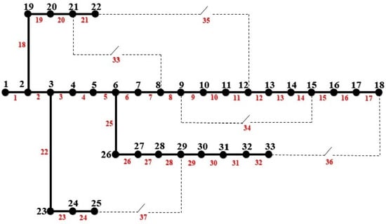
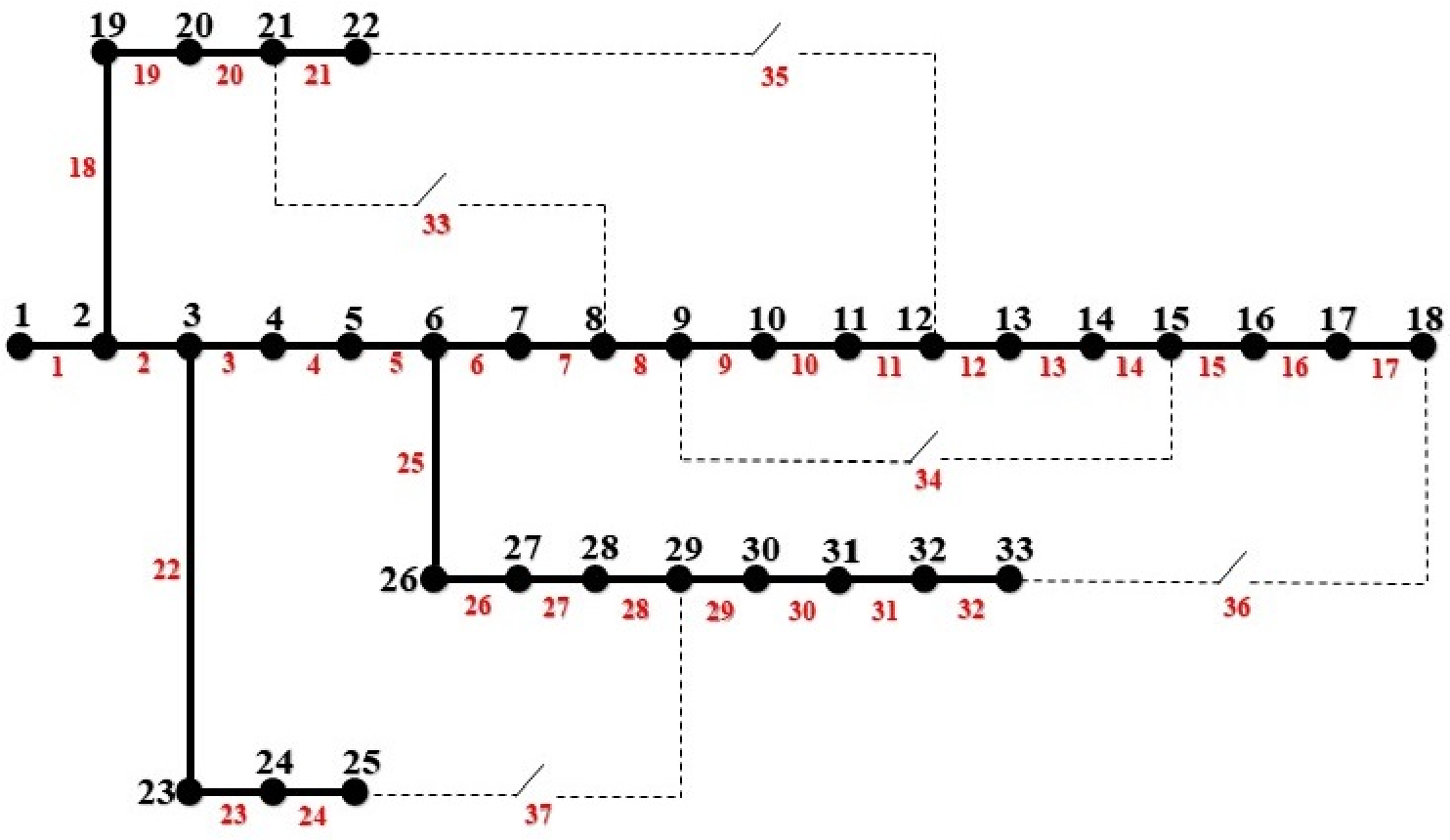
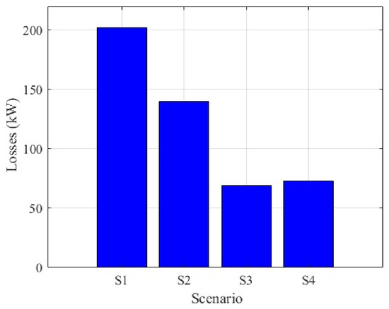
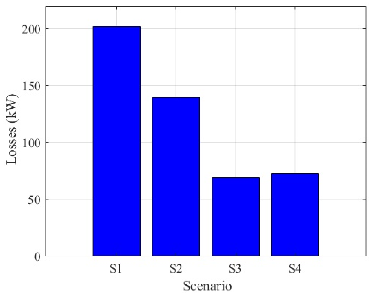
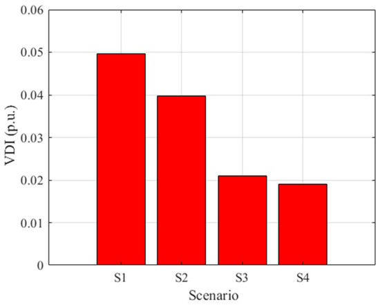
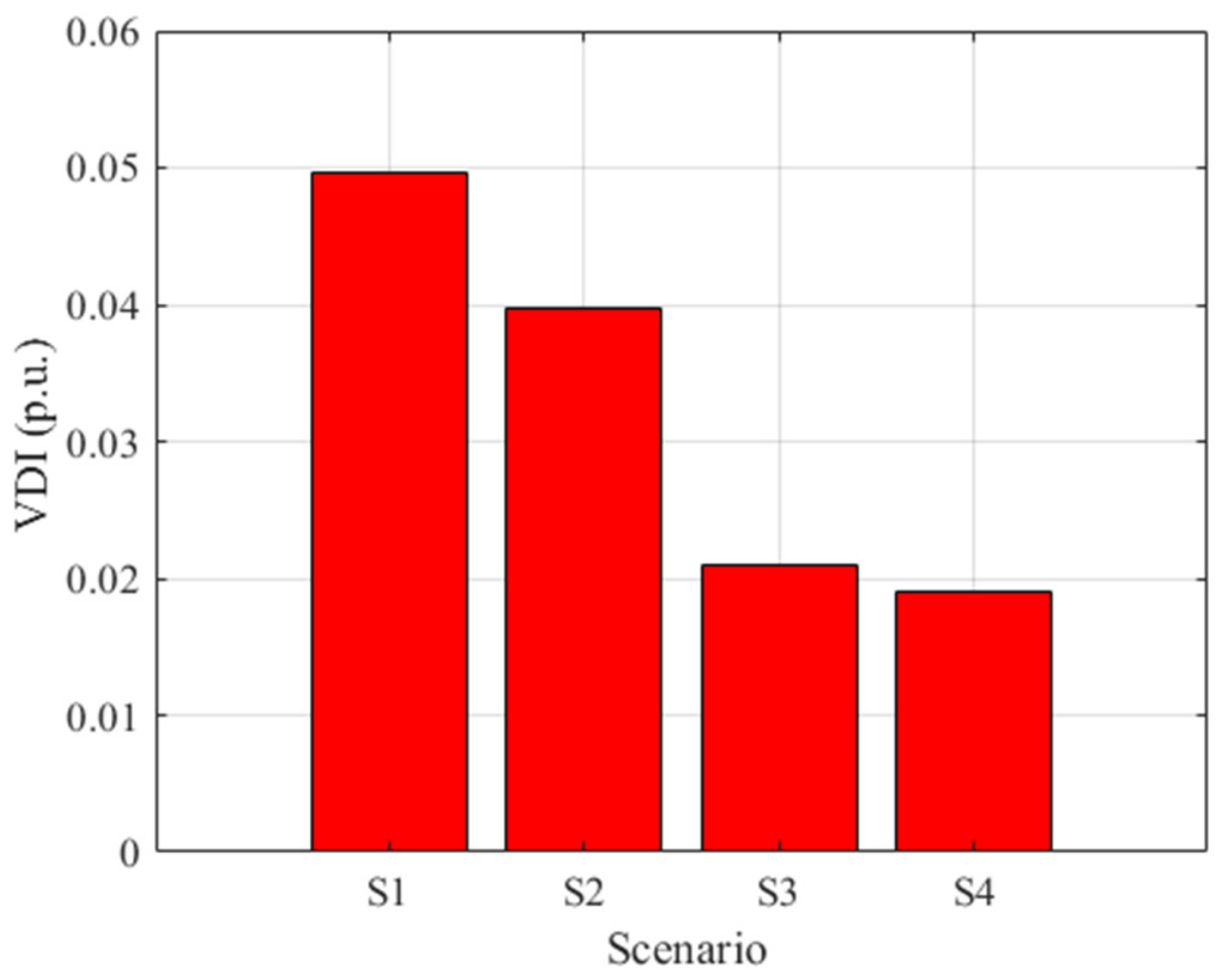
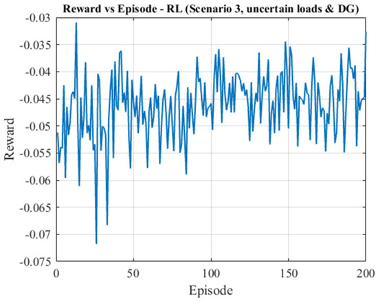
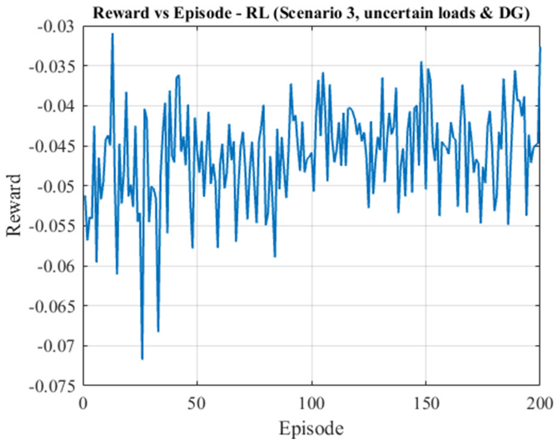
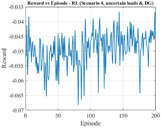
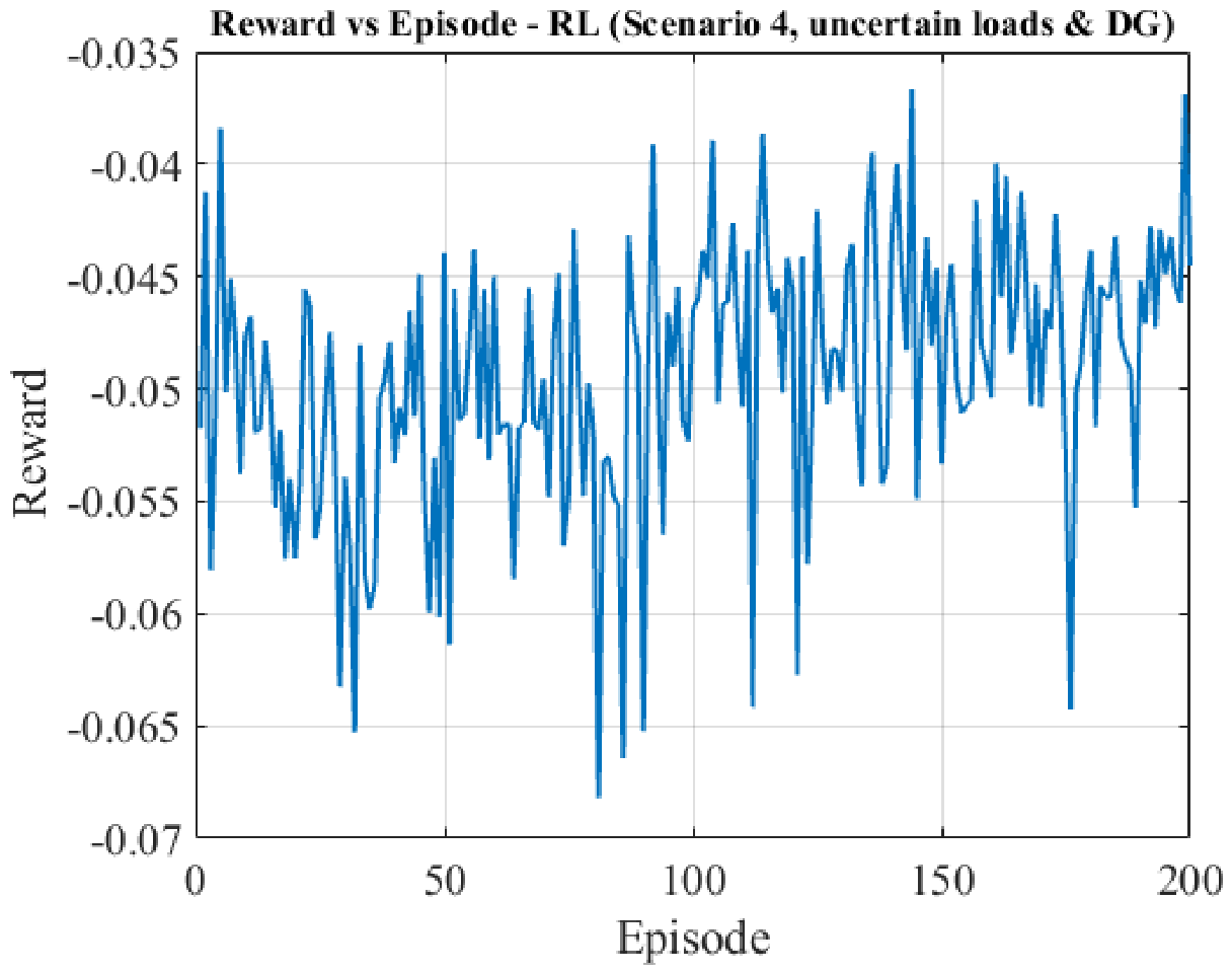
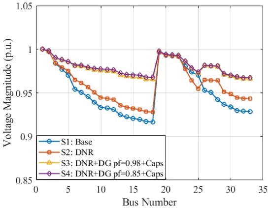
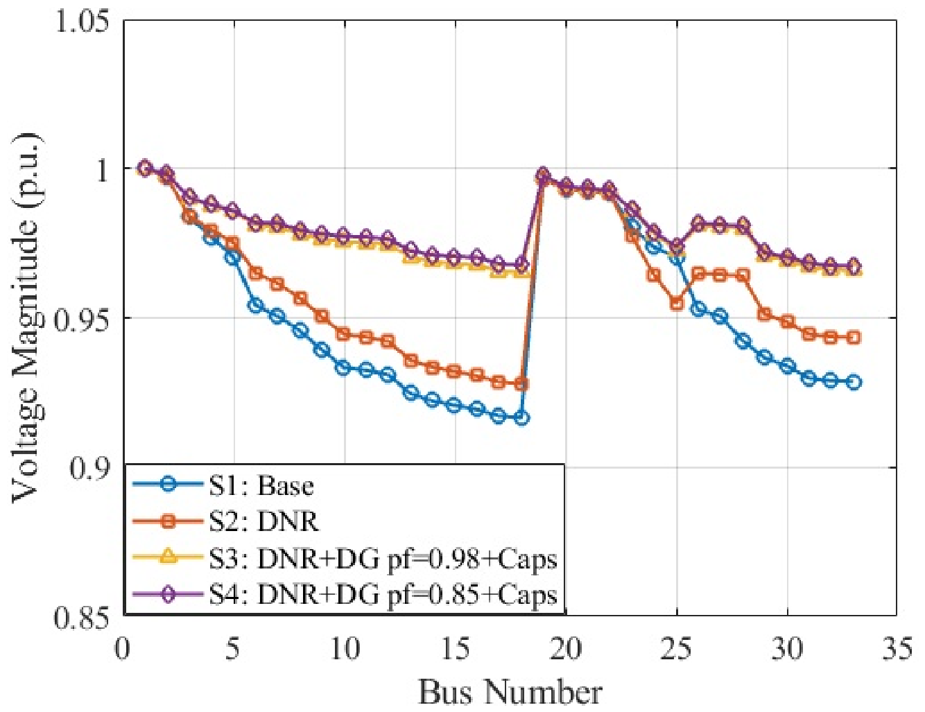
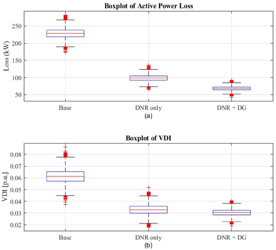
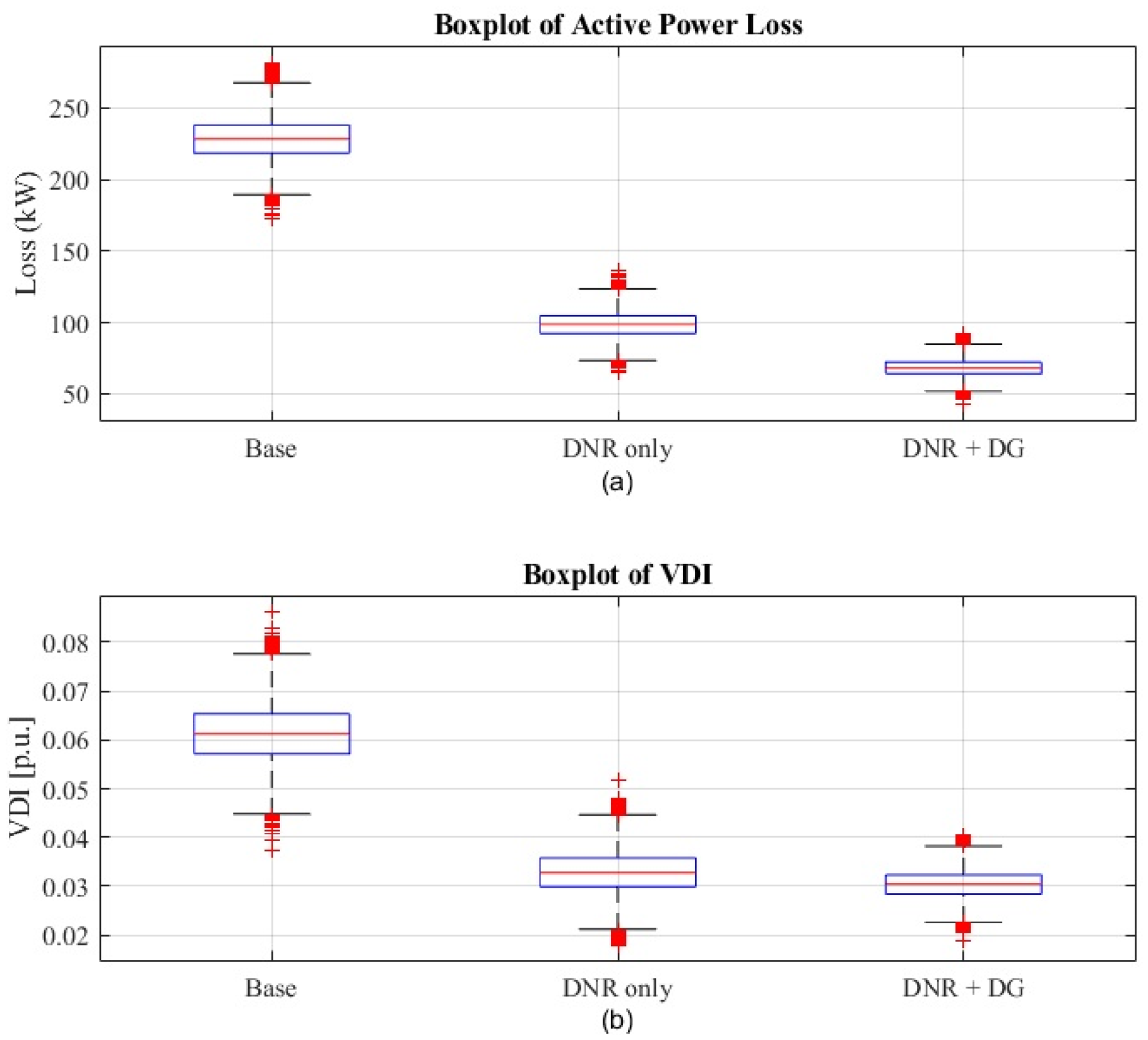
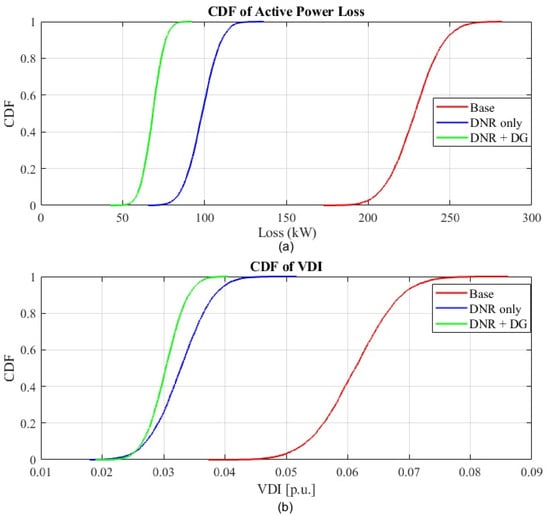
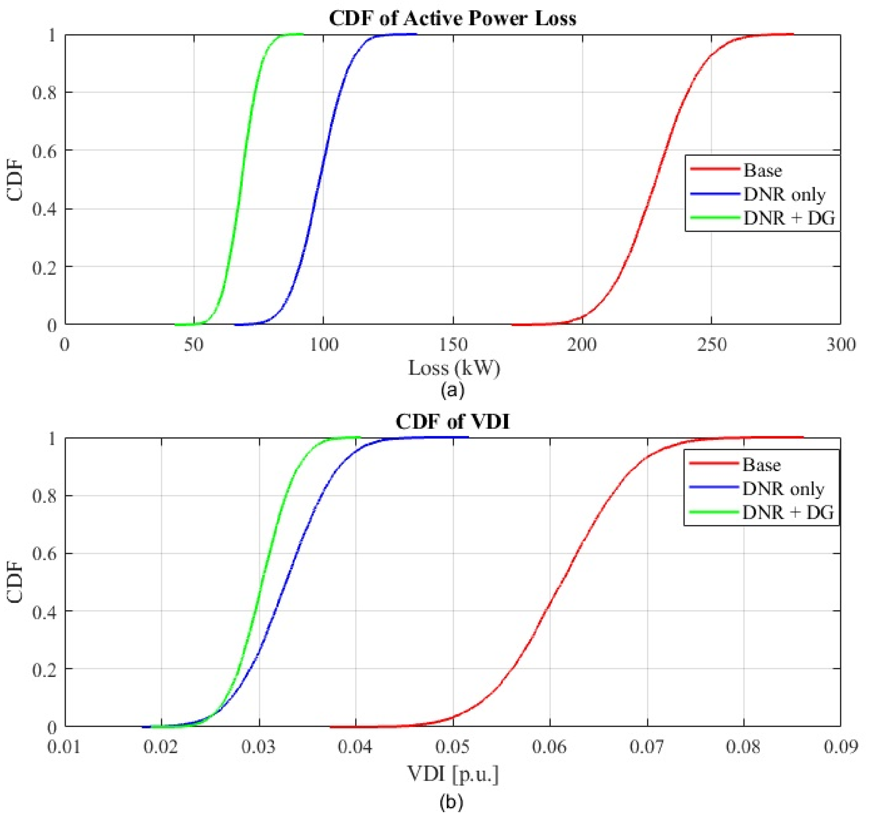

Disclaimer/Publisher’s Note: The statements, opinions and data contained in all publications are solely those of the individual author(s) and contributor(s) and not of MDPI and/or the editor(s). MDPI and/or the editor(s) disclaim responsibility for any injury to people or property resulting from any ideas, methods, instructions or products referred to in the content. |
© 2026 by the author. Licensee MDPI, Basel, Switzerland. This article is an open access article distributed under the terms and conditions of the Creative Commons Attribution (CC BY) license.