Predicting Football Match Outcomes Using Machine Learning

Abstract

Football match outcomes are influenced by a complex interplay of dynamic team strategies and stochastic match events, posing a significant challenge for predictive analytics. In this paper, we present a unified benchmarking study for football match outcome classification, using a dataset of 225,474 matches spanning 2018–2026 and a strictly chronological train–test split. Six classifiers spanning several modelling approaches, Logistic Regression, Generalized Additive Models, FastTree, Random Forest, Radial Basis Function networks and Multi-Layer Perceptron, are trained and evaluated under identical conditions. Bookmaker odds are converted into margin-free probabilities by the power method, with the exponent found by the Newton–Raphson method, and are included among the input features. In addition to the six classifiers, we also report a majority-class baseline and the de-vigged bookmaker prediction itself. Results are reported for both a binary one-vs-rest formulation and the original three-class (1, X, 2) formulation, with 95% bootstrap CIs for every metric and every model. Across the six classifiers, the differences are small: macro-averaged Precision ranges from 64.83% to 65.16% for Home Win and from 68.05% to 68.46% for Away Win, and macro-averaged Recall from 63.16% to 63.51% and from 59.10% to 59.72%, respectively, with substantially overlapping confidence intervals. In the three-class formulation, models trained without market data reach 48.0% accuracy against 43.4% for a trivial baseline and 51.9% for the bookmaker. Models trained with market data match the bookmaker but do not improve upon it on log-loss, Brier score or the ranked probability score. The only statistically distinguishable improvement of any kind is a 0.086 point accuracy advantage for the additive model, which is not accompanied by any improvement in the proper scoring rules and therefore does not indicate a practical advantage. Probability calibration and betting-signal generation are outside the scope of this study.

1. Introduction

Machine learning (ML) methods are now applied across a wide range of scientific and applied fields, from the physical sciences [1,2,3,4,5,6] to medicine [7,8] and economics [9,10], and the tools most often used are neural networks (NNs) [11,12,13,14], decision trees (DTs) [15,16] and support vector machines (SVMs) [17,18]. In this research study, we address the problem of predicting the outcome of a football match by examining it through a variety of ML techniques. This problem has been addressed in a number of earlier studies.

Predicting football match outcomes is difficult because of the high levels of noise, changing team strategies and unpredictable match events. Standard predictive models often struggle in these volatile environments. This research is important for three main reasons. First, we conduct a rigorous comparative analysis. Instead of focusing on just one algorithm, we compare different classifiers on the same input space. This provides a controlled comparison of how each model handles the non-linearity and volatility of sports data. Second, we report results for both a binary one-vs-rest decomposition and the original three-class outcome, using metrics that do not depend on an arbitrary decision threshold. Third, and central to this study, we evaluate all models against the de-vigged bookmaker forecast. Because market prices already aggregate team strength, recent form and public information, a benchmark that omits them cannot establish whether a model contributes new information or simply reproduces the bookmaker’s choice [19,20]. Reporting such a comparison also calls for restraint in what is claimed from model outputs, a concern documented in forecasting settings beyond sport [21].

For example, Hvattum et al. proposed the incorporation of ELO ratings for the prediction of match outcomes in their study [22]. Also, Owramipur et al. used Bayesian networks [23] to predict the outcomes for the Spanish League Barcelona team [24]. Similarly, Prasetio et al. proposed the incorporation of Logistic Regression [25] to predict the outcomes of football matches [26]. Moreover, Martins et al. used a polynomial classifier for the prediction of football outcomes [27]. Schauberger et al. selected the method of random forests (RFs) to predict the results of football matches in their study [28]. Player-level attributes were studied by Danisik et al. for the same purpose [29]. Constantinou proposed a new ML model, named Dolores, which is based on Hybrid Bayesian Networks, to predict football match outcomes from datasets selected in a series of countries [30]. Baboota et al. applied gradient boosting [31] to the English Premier League [32]. Additionally, Rahman proposed a deep learning framework for the same problem [33].

To address the limitations of individual algorithms in sports forecasting, we present a unified benchmarking study. Our methodology rests on two elements:

• A Consistent Feature Engineering Pipeline: We build a predictive feature vector that combines dynamic team performance indicators—such as Elo ratings [22], Home Clean Sheet and Away Fail-To-Score ratios—with raw bookmaker market odds. These odds are converted to margin-free market probabilities by the power method, with the exponent solved by the Newton–Raphson method [34].
• Comprehensive Architectural Benchmarking: We conduct a comparative evaluation of different classifiers under the same conditions. By testing models ranging from linear approaches (Logistic Regression) and generalized additive frameworks (Generalized Additive Models (GAM)) to tree structures (FastTree, RF) and NN models (Multilayer Perceptron (MLP), Radial Basis Function (RBF) networks), we provide a controlled comparison across different modelling mechanisms.

Overall, the proposed framework provides a fully specified methodology for evaluating several classifiers under identical experimental conditions. The experimental results indicate that the six classifiers perform almost identically once they are evaluated under a common protocol with confidence intervals (CIs). What separates the predictors is not the choice of algorithm but the comparison with the two reference predictors. These findings support the systematic evaluation of predictive models for football match forecasting under a common experimental protocol.

Although numerous studies have reported promising results for football match prediction, direct numerical comparison remains challenging because different datasets, leagues, feature sets and evaluation protocols are typically employed. Rather than claiming a universally superior predictive accuracy, the present work focuses on providing a unified and fully specified benchmarking framework in which six classifiers spanning several modelling approaches are evaluated under identical experimental conditions on a large-scale dataset. This allows a fair assessment of their relative performance using metrics that do not depend on arbitrary decision thresholds, with CIs obtained by bootstrap resampling, and against explicit reference predictors.

The main contributions of this work can be summarized as follows:

1.

A large-scale classification benchmark in which six classifiers are trained and evaluated under identical experimental conditions on 225,474 matches, using a feature space that is identical across the six classifiers and chronological train–test split.

2.

An evaluation against two reference predictors: a trivial majority-class baseline and the de-vigged bookmaker probability treated as a classifier. In both outcome formulations, all six classifiers are additionally estimated without odds-based inputs, which isolates the contribution of the remaining features.

3.

Results for both a binary one-vs-rest decomposition and the original three-class outcome, reported with proper scoring rules (log-loss, Brier score, ranked probability score) and 95% bootstrap CIs for all six classifiers.

4.

A time-sensitive feature construction pipeline explicitly preventing leakage, and a permutation-importance analysis identifying which engineered features contribute to predictive performance and which do not.

The remainder of this article is organised as follows: In Section 2, the dataset and the methodology are described, in Section 3, the experimental results are outlined, and finally, in Section 4, a discussion is provided based on the experimental results.

2. Materials and Methods

In this study, we use a large-scale dataset of historical football matches. The match results and pre-match odds were collected from the publicly accessible pages of OPAP, the licensed operator of fixed-odds sports betting in Greece, by automated retrieval carried out for this study. For each match, the records contain the final score, the identity of the two teams and the competition, and a single pre-match quotation for the home-draw-away market together with several ancillary markets. The automated retrieval formed part of a scientific text-and-data-mining workflow conducted within the research activities of the authors’ universities, and relies on the mandatory exception for text and data mining for the purposes of scientific research by research organisations, introduced into Greek law by Article 21A of Law 2121/1993 as added by Law 4996/2022, transposing Article 3 of Directive (EU) 2019/790. De-vigging uses the power method: the reciprocals of the three decimal odds are raised to the exponent that makes them sum to one, solved by the Newton–Raphson method from a starting value of one, with a tolerance of 1 × ${10}^{-13}$ and, at most, sixty iterations. The data include not only match results but also team-level performance indicators and pre-match market odds.

Figure 1 summarises the complete experimental pipeline, from the raw match records through feature construction and the chronological split to the evaluation protocol. All historical features are built under a strict point-in-time rule, described in detail below. The same benchmark feature set is used in all performance comparisons: the binary and the three-class formulations differ only in how the outcome is encoded, and each of them is estimated both with and without the market probabilities among the inputs. This way, it is possible to separate the contribution of the engineered features from the information already contained in the odds.

Figure 1. Overview of the experimental methodology. Historical features are constructed under a strict point-in-time rule. Both the binary one-vs-rest and the three-class formulations are estimated on an identical feature space, with and without the market probabilities among the inputs, and every result is compared against a majority-class baseline and the de-vigged bookmaker forecast.

The experimental dataset comprises 225,474 match events spanning from 20 October 2018 to 28 February 2026. The records cover a large number of competitions, identified in the source by 583 distinct competition codes of widely varying size, from major national first divisions to competitions represented by only a handful of fixtures. All of them are included in the pooled training and test sets. To ensure rigorous evaluation, the data were partitioned into a training set of 149,979 matches and a dedicated test set of 75,495 matches. The raw variables and the candidate-derived features are summarised in Table 1. Neither LeagueId nor SeasonPhase is supplied to the models as an input: the first would let a model identify the competition rather than assess the fixture, and the second was found to contribute nothing in the feature-importance analysis reported below. To avoid information leakage and better reflect a real-world deployment scenario, the dataset was partitioned chronologically, with earlier seasons used for training and later matches reserved exclusively for testing.

Table 1. Raw variables and candidate derived features considered in the study, with the role of each in the analysis. The final benchmark feature set is the one specified in the experimental results subsection; the ratio forms and SeasonPhase were candidates that the feature-importance analysis excluded.

Feature	Description/Range	Role in Analysis
MatchDate	Temporal identifier (2018–2026)	Raw record; not an input
League/LeagueId	Categorical identifiers for competitive tiers	Raw record; not an input
HomeTeam/AwayTeam	Competing squad identifiers	Raw record; not an input
Label	Primary outcome target (1, X, 2)	Prediction target
EloDiff	Difference in Elo ratings ($-500$ to $+500$)	Final benchmark
ProbHome/Draw/Away	Pre-match market probabilities (0 to 1)	Final benchmark (odds designs)
RankDifference	Difference between the three-level ranking tiers of the two teams as recorded in the source, away minus home (values −2 to +2)	Final benchmark
SeasonPhase	Categorical marker for season stage	Candidate; excluded
AttackVsDefense/DefenseVsAttack	AvgHs/(AvgAc + e) and AvgHc/(AvgAs + e): candidate ratio forms, not retained	Candidate; excluded
TotalScoringPotential	AvgHs-AvgAs: difference between the two teams’ rolling goal averages	Final benchmark
TotalDefensiveWeakness	AvgHc/(AvgAc + e): ratio of the two teams’ rolling goals-conceded averages	Candidate; excluded
HomeCleanSheetRatio	Probabilistic historical clean sheet frequency	Final benchmark
AwayFTSRatio	Away team Failed-to-Score probability	Final benchmark
AvgHs/AvgHc/AvgAs/AvgAc	Rolling goal averages over the last five venue-specific matches (scored and conceded, home and away)	Final benchmark
AttackMinusDefense/DefenseMinusAttack	AvgHs-AvgAc and AvgHc-AvgAs: stable difference forms of the corresponding ratios	Final benchmark
DefensiveWeaknessDiff	AvgHc-AvgAc: stable difference form of TotalDefensiveWeakness	Final benchmark
HistHome/HistAway	Number of prior matches at the relevant venue available for each team, 0 to 5 (data availability)	Final benchmark
Imputed	Indicator that the historical features of the match were imputed	Final benchmark

To capture the dynamic interaction between offensive and defensive capacities, the raw data were transformed into formal performance metrics. Let $Avg{H}_s$ and $Avg{H}_c$ denote the average goals scored and conceded by the home team, and $Avg{A}_s,Avg{A}_c$, the corresponding values for the away team. A smoothing constant $ϵ=0.01$ was applied to prevent division by zero. Hence, the following equations define the composite quantities that were constructed. Two functional forms were evaluated for the interaction between attack and defence, a ratio and a difference; the ratio forms are given first and were excluded from the benchmark in favour of their difference counterparts for the reasons reported in the feature-importance subsection:

1.

AttackVsDefense: a candidate ratio form, representing the home team’s offensive efficiency relative to the away team’s defensive record:

$$\mathrm{AttackVsDefense}={\displaystyle \frac{Avg{H}_s}{Avg{A}_c+ϵ}}$$

(1)

This feature measures how effectively the home team scores relative to the average number of goals conceded by its opponent.

2.

DefenseVsAttack: a candidate ratio form, quantifying the home team’s defensive capability against the away team’s scoring force:

$$\mathrm{DefenseVsAttack}={\displaystyle \frac{Avg{H}_c}{Avg{A}_s+ϵ}}$$

(2)

This feature describes the defensive capability of the home team relative to the offensive strength of the away team.

3.

TotalScoringPotential: modelled as the numerical difference between home and away scoring capacities, identifying the relative offensive edge:

$$\mathrm{TotalScoringPotential}=Avg{H}_s-Avg{A}_s$$

(3)

This metric provides the scoring potential of the two teams.

4.

TotalDefensiveWeakness: a candidate ratio form, assessing the relative vulnerability of the home defense compared to the away defense:

$$\mathrm{TotalDefensiveWeakness}={\displaystyle \frac{Avg{H}_c}{Avg{A}_c+ϵ}}$$

(4)

This feature compares the average goals conceded by the home and away teams.

5.

HomeCleanSheetRatio (HCSR) and AwayFTSRatio (AFTS) capture probabilistic historical frequencies:

$$HCSR={\displaystyle \frac{{\sum }_{i=1}^N\mathbb{I}(G_{H,c}=0)}{N}},AFTS={\displaystyle \frac{{\sum }_{j=1}^N\mathbb{I}(G_{A,s}=0)}{N}}$$

(5)

The HCSR represents the historical frequency with which the home team has prevented its opponent from scoring. Also, the AFTS represents the historical probability that the away team fails to score. In both, N is the same window of five venue-specific matches used for the goal averages.

6.

AttackMinusDefense, DefenseMinusAttack and DefensiveWeaknessDiff are the difference-form counterparts of the three ratios above, defined as AvgHs-AvgAc, AvgHc-AvgAs and AvgHc-AvgAc, respectively. Together with TotalScoringPotential, they are the four interaction features used in the benchmark. Unlike the ratios, they remain bounded when a denominator approaches zero, which is the property that motivated the comparison between the two forms.

Feature construction follows a strict point-in-time rule: for a match played on date t, every historical feature is computed using only matches with date strictly earlier than t. Because the source records match dates without kick-off times, the procedure operates one calendar day at a time—all features for a given day are computed from the state preceding that day, and the state is updated only afterwards, so that matches played on the same day cannot inform one another. Averages are taken over the last five matches of each team at the relevant venue, that is, home matches for the home team and away matches for the away team.

Matches for which fewer than five prior matches are available (22.4% of the dataset) are completed using the point-in-time mean of the same competition, computed only from earlier matches, with a global mean and a fixed prior as successive fallbacks, both of which are themselves computed only from matches earlier than the one being completed. A binary indicator is retained and supplied to the models as a feature. A static full-period mean was deliberately avoided, since it would use future matches to complete earlier ones. Because the ratio features become numerically unstable when the denominator approaches zero, they were winsorised at the 99.9th percentile of the training set, the threshold being computed on the training period alone and then applied unchanged to both periods. No class resampling was applied; the observed distribution of outcomes is the quantity being modelled.

Two checks were carried out to confirm that no information from the test period enters the training data. First, matches were matched between the two sets on the key formed by date, home team and away team; no match appears in both, and the unique record identifiers are likewise disjoint. Second, the Elo ratings were examined for the warm-up behaviour that a correctly sequential computation must exhibit. At a team’s first appearance, the rating difference has a standard deviation of 39 points, rising to 99 points once at least twenty prior matches have been observed; a rating computed with hindsight would show no such widening.

Rolling windows and Elo ratings are carried forward across season boundaries without reset: a team entering a new season retains the state accumulated in the preceding one, so that the first fixtures of a season are informed by the end of the previous campaign rather than being treated as if no history existed. Teams appearing in the data for the first time, including newly promoted sides, therefore begin with no history and are handled by the imputation rule described above. As regards the market data, the records contain a single pre-match odds snapshot per fixture. The source does not record the time at which that snapshot was taken, so we cannot state whether it corresponds to an opening, an intermediate or a closing quotation, and we do not assume one; the consequence is that neither odds movement nor closing-line value can be examined here, and this is noted among the limitations.

The generated feature space is explicitly designed to satisfy three essential, complementary operational criteria:

1.

Long-term structural team performance using rating systems (EloDiff, RankDifference). These features describe the relative competitive strength of the two teams and their position within their respective competitions.

2.

Interaction between offensive and defensive records (AttackMinusDefense, DefenseMinusAttack, TotalScoringPotential, DefensiveWeaknessDiff). These features contrast what each team scores with what its opponent concedes.

3.

Distribution-based prior probabilities derived from betting market evaluations (ProbHome, ProbDraw, ProbAway). These features provide an external assessment of the expected match outcome based on the betting market.

3. Results

3.1. Experimental Setup

The benchmark reported in this paper was implemented in Python using the scikit-learn library. The estimators are, in the order used as follows throughout: HistGradientBoostingClassifier for FastTree and for the additive model, the two differing in the number of iterations, the leaf count and the depth limit, with the additive model restricted to depth one (that restriction is why the second configuration is labelled GAM: trees of depth one can each use only a single feature, so the fitted function is a sum of univariate terms and the model is additive in the inputs—it is not a spline-based generalized additive model—and the label denotes the additive structure rather than the estimation method); RandomForestClassifier; LogisticRegression; MLPClassifier with a single hidden layer; and RBFSampler followed by LogisticRegression, which approximates a Gaussian kernel by random Fourier features.

Table 2 summarises the six classifiers compared in this study, each with its operating principle, the properties that motivate its inclusion, and the limitations that are relevant to the present task. The selection deliberately spans different inductive biases: a purely linear model, an additive non-linear model, a boosted-tree ensemble and a bagged one, a global non-linear approximator, and a kernel-approximation model. The purpose is not to identify a winner but to establish whether the choice among these classifiers materially affects predictive performance once the experimental conditions are held fixed.

Table 2. Functionality, advantages and limitations of the six benchmarked classifiers.

Method	Functionality	Advantages	Limitations
Logistic Regression	Linear model of the log-odds of the outcome, fitted by penalised maximum likelihood.	Few parameters, deterministic given the data, direct probabilistic outputs and interpretable coefficients.	Cannot represent interactions or non-monotone effects unless these are supplied explicitly; sensitive to heavy-tailed inputs.
GAM	Sum of univariate shape functions, one per feature, estimated here by depth-one gradient boosting [35].	Captures non-linear effects while remaining additive and inspectable per feature; robust to feature scaling.	Interactions between features are excluded by construction.
FastTree	Gradient-boosted decision trees, fitted stage-wise on the residuals of the current ensemble [36].	Handles non-linearity and interactions, tolerant of monotone transformations and of outliers, strong on tabular data.	Many hyperparameters; can overfit without regularisation; individual trees are not interpretable.
RF	Bagged ensemble of decision trees, each fitted on a bootstrap sample with a random subset of features at each split [37].	Low variance, little tuning required, naturally parallel, resistant to outliers.	Probability estimates are averages of leaf frequencies and tend to be less sharp; large memory footprint.
MLP	Feed-forward neural network with a single hidden layer of non-linear units, optimised by the Adam stochastic gradient method with early stopping [13].	Represents smooth interactions among features without them being specified in advance.	Requires feature scaling, sensitive to initialisation and to heavy-tailed inputs, and stochastic across seeds.
RBF network	Approximation of a Gaussian kernel by random Fourier features, followed by a linear classifier on the resulting representation [38].	Gives access to a kernel decision boundary at a cost that grows linearly rather than quadratically in the number of matches.	Performance depends on the number of random features and on the kernel scale, the representation is stochastic given a fixed seed, and the expansion is highly sensitive to extreme feature values.

Numerical inputs are median-imputed and, for the linear, network and kernel models, standardised. Both steps are part of the estimator pipeline, so their parameters are estimated from the training data alone and merely applied to the test set; in the cross-validation of the sensitivity analysis, they are re-estimated within each training fold before being applied to the validation fold; the tree ensembles receive the raw values.

The Elo ratings use K = 20, an initial rating of 1500 and no home advantage term; the difference is taken as the home rating minus the away rating, the expected score of the home team is the logistic function of that difference divided by 400, a draw is scored as half a win for both teams, and the update is zero-sum, K times the difference between the realised and the expected score; the fixed prior used as the last imputation fallback is 0.30 for frequencies, 1.00 for ratios and 0.00 for differences and goal averages; and the chronological split falls on 9 September 2022. Any estimator parameter not listed in the settings table retains the default value of the version stated below; the quantity referred to as the kernel scale is the gamma parameter of the random Fourier feature mapping. The results were produced with Python 3.12.10, scikit-learn 1.9.0, NumPy 2.5.0 and pandas 2.3.3; the versions are stated because the default behaviour of some estimators depends on them, in particular, the automatic activation of early stopping in the histogram-based boosting implementation at this sample size. Every estimator that accepts a random state was given the fixed value 42.

Hyperparameter sensitivity was assessed by random search with expanding-window time-series cross-validation carried out entirely inside the training set. Twenty configurations were drawn for each classifier, and each was scored on three successive validation folds in which the model is fitted on an earlier segment of the training data and evaluated on the segment that follows it, so that the temporal ordering is preserved at every stage. The purpose of this search was not to identify a single winning configuration but to establish how sensitive performance is to the choice of hyperparameters. Within the ranges given below, the sensitivity of the validation area under the curve (AUC) to the choice of configuration differs markedly between classifiers. For five of the six, it is small: across the 20 configurations, the range is below 0.001 for Logistic Regression and the additive model, and at most 0.014 for FastTree, the RF and the MLP. It is larger elsewhere: 0.181 for the RBF network, driven almost entirely by one setting, the kernel scale (correlation −0.992), whose extreme values degrade performance sharply rather than improve it. The best configuration of every classifier lies between 0.7061 and 0.7098, a band of 0.004, so no choice within the ranges explored raises any classifier above it. No configuration of any classifier reaches the de-vigged market forecast, which scores 0.7104 on the same folds.

The results reported throughout this paper were therefore produced with the fixed configurations listed in Table 3. These are conventional settings for the implementations concerned. For the random-feature expansion, the one classifier in which the choice matters, the pre-specified kernel scale of 0.05 is not the best value drawn in the search, so the reported result is not a search optimum. The comparison between classifiers should therefore be read as a comparison at a reasonable configuration for each rather than as a claim that the configuration is immaterial, which the analysis establishes directly for the five classifiers whose range does not exceed 0.014. The values are pre-specified settings within the explored ranges, fixed in advance of the analysis rather than derived from it. The configuration for each classifier was held unchanged across both outcome formulations, and the same sensitivity-analysis protocol was applied to all six classifiers, so that no classifier is treated more favourably than another. The test set was not used at any point, either in the sensitivity search or in the specification of these values. Table 3 reports the fixed configurations used for the results presented here; the ranges explored were, for the tree ensembles, 100 to 800 boosting iterations, 15 to 127 leaves, learning rates from 0.02 to 0.2 and minimum leaf sizes from 20 to 200; for the RF, 200 to 400 trees with 31 to 511 leaves and feature fractions from 0.3 to 1.0; for the MLP, a single hidden layer with 10 to 128 units and L2 penalties from 1 × ${10}^{-5}$ to 1 × ${10}^{-2}$, optimised throughout with Adam and early stopping on an internal validation split; for the GAM, 100 to 600 boosting iterations with learning rates from 0.02 to 0.1 at depth one; for Logistic Regression, inverse regularisation strengths from 0.01 to 100; and for the RBF network, 100 to 1000 basis functions with kernel scales from 0.01 to 1.0. Where the reported implementation exposes a different parameterisation of the same quantity, Table 3 gives the values in the form used by that implementation. The search was carried out on the most recent 50,000 matches of the training set, which is stated here because it is a property of the sensitivity analysis and not of the reported results: the fixed configurations of the results tables were fitted on the full training set. The mild temporal shift visible in the decline of the bookmaker margin over the observation period is discussed with the limitations.

Table 3. Experimental settings.

Method	Parameter	Value
FastTree	Boosting iterations	300
FastTree	Maximum leaves	31
FastTree	Learning rate	0.05
FastTree	Minimum samples per leaf	100
GAM	Boosting iterations	300
GAM	Learning rate	0.05
GAM	Maximum depth	1
Logistic Regression	Inverse regularisation C	1.0
Logistic Regression	Maximum iterations	3000
RF	Trees	200
RF	Maximum leaves	127
RF	Minimum samples per leaf	20
RF	Feature fraction	0.8
MLP	Hidden units (single layer)	32
MLP	L2 penalty	0.0001
MLP	Optimiser	Adam
MLP	Early stopping	Yes (10% internal split)
MLP	Maximum iterations	300
RBF network	Basis functions	300
RBF network	Kernel scale	0.05
RBF network	Readout regularisation C	1.0

These parameters are analyzed in detail below:

1.

Boosting iterations: The number of successive trees added to a boosted ensemble. More iterations allow a closer fit but increase the risk of overfitting.

2.

Maximum leaves: The upper limit on the number of terminal nodes in a single tree, and hence on how many distinct regions of the feature space it can separate.

3.

Maximum depth: The longest path from root to leaf. A depth of one restricts the model to additive effects, with no interactions between features.

4.

Learning rate: The weight given to each successive tree. Lower values make the optimisation more stable but require more iterations to converge.

5.

Minimum samples per leaf: The smallest number of matches that a terminal node may contain. Higher values act as regularisation, preventing the model from fitting individual outliers.

6.

Trees: The number of trees grown independently in the bagged ensemble. More trees reduce variance at a proportional cost in training time.

7.

Feature fraction: The proportion of features considered at each split. Values below one introduce randomness across trees and improve generalisation.

8.

Hidden units: The width of the single hidden layer of the neural network, which determines how many non-linear basis functions the network can form.

9.

L2 penalty: The strength of the quadratic penalty on the network weights, controlling the trade-off between fit and smoothness.

10.

Optimiser: The numerical method used to minimise the training objective. Adam is a stochastic first-order method with adaptive per-parameter step sizes; training stops when the score on an internal validation split ceases to improve.

11.

Basis functions: The number of random Fourier features used to approximate the Gaussian kernel in the radial-basis network, following the construction of Rahimi and Recht [38].

12.

Kernel scale: The gamma parameter of the random Fourier mapping that approximates the Gaussian kernel. Smaller values produce a broader, smoother response over the feature space.

13.

Inverse regularisation strength: The reciprocal of the penalty applied to the coefficients of the linear models. Larger values correspond to weaker regularisation.

14.

Maximum iterations: The limit on the number of passes the optimiser may make over the training data before stopping.

3.2. Experimental Results

Before presenting the numerical results, it is important to clarify how the target variable was constructed for each market. The original dataset label (Label ∈ {1, X, 2}) corresponds to the three-way outcome of a match (home win, draw, away win). For the binary analyses reported below, the original three-class outcome was decomposed into three separate one-vs-rest classification problems, one for each outcome. The home win and away win markets are reported first, in the two tables that follow; the draw is reported separately below, because at the fixed threshold, it produces almost no positive predictions and its threshold-based figures are therefore uninformative:

1.

Home Win market (Table 4): The positive class corresponds to the outcome “1” (home win), while the classes “X” (draw) and “2” (away win) were merged into a single negative class, “not Home Win.” In other words, the model is asked to answer the question “will the home team win or not?”, collapsing the distinction between a draw and an away win.

Table 4. Home win experimental results. Each model cell gives the point estimate and, beneath it, the 95% bootstrap CI over 1000 paired resamples [39] of the test set. The two reference predictors are computed without training and are reported as point estimates.

Model	Error	Precision (Macro)	Recall (Macro)
Trivial (majority class)	43.45%	-	-
Bookmaker odds (de-vigged)	34.52%	65.04%	63.40%
FastTree	34.57% [34.21, 34.90]	65.03% [64.66, 65.42]	63.29% [62.96, 63.65]
GAM	34.54% [34.16, 34.86]	65.02% [64.67, 65.42]	63.37% [63.06, 63.74]
LogReg	34.50% [34.12, 34.82]	65.00% [64.65, 65.40]	63.51% [63.17, 63.87]
MLP	34.50% [34.13, 34.83]	65.16% [64.80, 65.54]	63.30% [62.97, 63.65]
RF	34.60% [34.24, 34.93]	64.99% [64.64, 65.37]	63.25% [62.93, 63.60]
RBF	34.73% [34.36, 35.06]	64.83% [64.48, 65.20]	63.16% [62.84, 63.51]

2.

Away Win market (Table 5): Conversely, the positive class corresponds to the outcome “2” (away win), while the classes “X” (draw) and “1” (home win) were merged into a single negative class, “not Away Win.”

Table 5. Away win experimental results. Each model cell gives the point estimate and, beneath it, the 95% bootstrap CI over 1000 paired resamples of the test set. The two reference predictors are computed without training and are reported as point estimates.

Model	Error	Precision (Macro)	Recall (Macro)
Trivial (majority class)	31.18%	-	-
Bookmaker odds (de-vigged)	27.86%	68.42%	59.28%
FastTree	27.89% [27.58, 28.21]	68.40% [67.91, 68.94]	59.18% [58.90, 59.50]
GAM	27.90% [27.59, 28.22]	68.46% [67.95, 68.99]	59.10% [58.82, 59.42]
LogReg	27.85% [27.52, 28.18]	68.08% [67.59, 68.60]	59.72% [59.44, 60.04]
MLP	27.83% [27.51, 28.16]	68.41% [67.92, 68.98]	59.37% [59.10, 59.69]
RF	27.86% [27.54, 28.20]	68.42% [67.93, 68.95]	59.28% [59.00, 59.60]
RBF	27.98% [27.66, 28.31]	68.05% [67.55, 68.59]	59.22% [58.93, 59.53]

The binary formulation is a one-vs.-rest decomposition of the three-class outcome, reported because the two merged markets are the form in which such predictions are most often presented. Each of the three binary probabilities is directly comparable with the corresponding de-vigged market probability for that one-vs.-rest task, and the tables below make that comparison. Their triplet, however, is not a coherent three-class distribution, because three independently fitted probabilities need not sum to one; the three-class formulation reported afterwards has that property by construction, and is therefore the formulation in which the multiclass scoring rules are applied. The operating threshold for all binary tasks is 0.5. We also note that the Precision and Recall values in Table 4 and Table 5 are macro averages across both classes rather than positive-class values, as indicated in the column headings.

The same benchmark feature set is used in all the primary performance comparisons reported in this paper. It comprises the three de-vigged market probabilities, the Elo difference and the ranking difference, the two counts of prior matches available for the two teams, together with the indicator recording whether historical values had to be imputed, the four rolling goal averages, four difference-form combinations of attacking and defensive strength, and two historical frequencies: 18 inputs in total, or 15 when the three market probabilities are withheld. The feature space is identical across all six classifiers and also identical between the binary and the three-class formulations, so that the two can be compared without any confounding from the inputs.

Table 4 depicts the experimental results using the incorporated method on the Home Win dataset.

Table 4 summarises the performance of the six classifiers on the binary “Home Win vs. merged X2” problem. The most notable feature of the table is how little the methods differ. Error ranges are from 34.50% to 34.73% and macro-averaged Precision from 64.83% to 65.16%, a spread of 0.23 and 0.33 percentage points, respectively, across the six classifiers. MLP records both the lowest error (34.50%) and the highest Precision (65.16%), but the bootstrap CIs of these quantities overlap for every pair of models, so the ordering should not be interpreted as a ranking. The comparison that does separate the predictors is the one with the two reference rows: all six classifiers improve substantially on the majority-class baseline (43.45% error), and all six coincide with the de-vigged bookmaker forecast (34.52% error) to within 0.21 percentage points. Similarly, Table 5 presents the experimental results on the Away win dataset.

In the binary “Away Win vs. merged X1” problem, error ranges are from 27.83% to 27.98% across the six classifiers and macro-averaged Precision from 68.05% to 68.46%, with GAM attaining the highest Precision and MLP the lowest error. Again the differences are smaller than the width of the corresponding CIs. The bookmaker reference records 27.86% error and 68.42% Precision, values that fall inside the range spanned by the models; the majority-class baseline records 31.18% error. The absolute error level is lower than in the Home Win market because away wins are the less frequent outcome, which mechanically reduces the error of a conservative classifier. The same rarity shows in the positive class: at the 0.5 threshold, the classifiers recover between 24.5% and 26.7% of away wins, against between 46.5% and 48.3% of home wins at comparable positive-class Precision, so the macro averages reported here should be read together with the F1 column of the additional metrics tables. Taken together, Table 4 and Table 5 show the same picture in both merged binary formulations: the models show small differences in Precision and Recall at the fixed 0.5 threshold, but no classifier holds a consistent advantage in both quantities: the highest macro Precision is attained by MLP in the Home Win market and by GAM in the Away Win market, while the highest macro Recall is attained by Logistic Regression in both markets, which also has the second-lowest Precision in both. The CIs of these leaders overlap with those of the classifiers immediately behind them, so none of these orderings is distinguishable. What differences there are reflect where each classifier’s probabilities fall relative to the common 0.5 cut-off rather than any difference in discriminative ability: the models with higher Recall record correspondingly lower Precision, while their AUC values are very close and their bootstrap CIs overlap substantially. The threshold-free comparison in the following Section 3.3, therefore addresses the question directly, with the six classifiers and the two reference predictors placed side-by-side on both markets. The results reported so far include the de-vigged market probabilities among the inputs. Table 6 repeats the two binary markets with those three columns removed, so that the contribution of the engineered features can be read on its own. Everything else, the chronological split, the fixed configurations and the evaluation protocol, is unchanged.

Table 6. Binary results with the odds-based features removed. Error is reported at the fixed 0.5 threshold and AUC is threshold-free. The two reference rows do not depend on the model inputs and are repeated from the preceding tables so that the comparison can be read within a single table. Each model cell gives the point estimate and, beneath it, the 95% bootstrap CI over the same 1000 resamples of the test set.

Model	Home Win Error	Home Win	Away Win Error	Away Win
Trivial (majority class)	43.45%	-	31.18%	-
Bookmaker odds (de-vigged)	34.52%	0.7052	27.86%	0.7139
FastTree	38.10% [37.77, 38.45]	0.6466 [0.6426, 0.6502]	30.06% [29.72, 30.37]	0.6515 [0.6476, 0.6559]
GAM	38.10% [37.75, 38.47]	0.6467 [0.6426, 0.6503]	30.05% [29.73, 30.37]	0.6510 [0.6471, 0.6553]
LogReg	38.26% [37.93, 38.62]	0.6477 [0.6437, 0.6514]	30.08% [29.75, 30.41]	0.6522 [0.6482, 0.6567]
MLP	38.34% [38.00, 38.72]	0.6464 [0.6424, 0.6500]	30.03% [29.70, 30.36]	0.6510 [0.6470, 0.6553]
RF	38.09% [37.76, 38.44]	0.6466 [0.6425, 0.6503]	30.11% [29.76, 30.44]	0.6516 [0.6476, 0.6560]
RBF	38.18% [37.84, 38.53]	0.6461 [0.6421, 0.6499]	30.08% [29.75, 30.39]	0.6514 [0.6476, 0.6558]

Removing the market probabilities moves every model in the same direction and by a similar amount. Error rises from 34.50–34.73% to 38.09–38.34% in the Home Win market and from 27.83–27.98% to 30.03–30.11% in the Away Win market, while AUC falls from 0.7023–0.7051 to 0.6461–0.6477 and from 0.7108–0.7136 to 0.6510–0.6522, respectively. The six classifiers remain as close to one another as before, which is the point of the comparison: the drop is caused by the removal of an input, not by the choice of algorithm. Measured against the two reference rows, the best model without market information covers 60% of the distance from the majority-class baseline to the bookmaker in the Home Win market and 35% in the Away Win market. For the draw outcome, the same removal lowers AUC to 0.5350–0.5476, against 0.5843 for the market, confirming that this outcome carries the least information of the three. No model attains a higher AUC than the market in either design, and the same holds for the logarithmic loss, the Brier score and the ranked probability score (RPS) in the three-class tables below.

3.3. Statistical Comparison of the Experimental Results

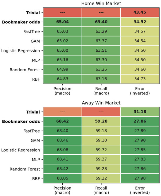
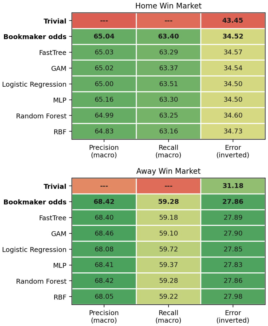
The two binary markets are summarised together in Figure 2, which reports the same three quantities as Table 4 and Table 5 for the six classifiers and for the two reference predictors on a single colour scale.

Figure 2. Macro-averaged Precision, Recall and Error (%) for the six classifiers and the two reference predictors, on the Home Win (top) and Away Win (bottom) markets. The colour scale is absolute and identical for both markets, so that differences of a few tenths of a point between models appear as differences of a few tenths. The Error column is colour-inverted (100—Error) so that green denotes better performance throughout; the numeric labels give the actual values.

The heatmap condenses the results of the two binary markets into a single panel. Its main message is the uniformity of the colouring: the six classifiers occupy a narrow band in every column, and no row is systematically greener than the others.

Five of the six classifiers are stochastic given fixed training data, so the values reported in the tables above depend to some extent on the random seed. Table 7 quantifies that dependence over 30 refits of each stochastic classifier; Logistic Regression was refitted twice, to confirm that it is deterministic. The standard deviation of the error lies between 0.012 and 0.066 percentage points, which is small in absolute terms but not negligible relative to the differences between classifiers: the means themselves span 0.146 percentage points in the Home Win market, so seed variation does not by itself account for the ordering of the classifiers. What it does account for is the distance to the market. In the Home Win market, the error of the de-vigged bookmaker forecast falls inside the range of the 30 refits for four of the six classifiers, and in the Away Win market for five of the six, while 14 of the 15 pairs of classifiers have overlapping ranges in the Home Win market and 13 of 15 in the Away Win market. The observed gap between neighbouring classifiers is therefore of the same order as the variation induced by the seed alone, and should not be over-interpreted. The values printed in the results tables were produced with a single fixed seed, and they fall within or immediately adjacent to the ranges reported here.

Table 7. Sensitivity of the reported error to the random seed. Each stochastic classifier was refitted 30 times on the full training set with a different seed and evaluated on the test set; the table gives the mean error, its standard deviation and the range observed across those fits. Logistic Regression is deterministic given fixed training data and was refitted twice to confirm it. The reference row is repeated from the preceding tables and does not depend on training.

Model	Home Win Mean Error	Home Win SD [Min, Max]	Away Win Mean Error	Away Win SD [Min, Max]
Bookmaker odds (de-vigged)	34.52%	-	27.86%	-
FastTree	34.577%	0.044 [34.487, 34.680]	27.884%	0.025 [27.834, 27.936]
GAM	34.507%	0.027 [34.457, 34.597]	27.875%	0.012 [27.850, 27.892]
LogReg	34.500%	0 [34.500, 34.500]	27.847%	0 [27.847, 27.847]
MLP	34.602%	0.054 [34.490, 34.678]	27.899%	0.061 [27.816, 28.087]
RF	34.590%	0.029 [34.548, 34.687]	27.842%	0.017 [27.814, 27.884]
RBF	34.646%	0.066 [34.475, 34.757]	27.963%	0.051 [27.855, 28.085]

The results tables report the three quantities on which the comparison with the market turns. For completeness, Table 8 and Table 9 give five further metrics for both binary markets, each with its 95% bootstrap CIs: the two threshold-free measures of ranking quality, the F1-score of the positive class, and the Brier score and logarithmic loss. The pattern is the one already described. Every interval for every model overlaps the corresponding value for the de-vigged market forecast on the probabilistic scores, and no model attains a higher AUC or average Precision than the market in either market.

Table 8. Additional metrics for the Home Win market, with 95% bootstrap CIs. The three quantities reported in the corresponding results table above are not repeated here. Precision and Recall for the positive class are summarised by the F1 column; their macro-averaged counterparts are in Table 4. Intervals are percentile intervals over 1000 resamples of the test set, computed from the same resamples for every predictor so that the comparisons are paired.

Predictor		Average Precision	F1 (Positive)	Brier	Log Loss
Bookmaker odds (de-vigged)	0.7052	0.6486	54.47%	0.2137	0.6149
FastTree	0.7047 [0.7012, 0.7085]	0.6478 [0.6427, 0.6535]	54.14% [53.64, 54.64]	0.2139 [0.2128, 0.2150]	0.6154 [0.6129, 0.6178]
GAM	0.7050 [0.7013, 0.7087]	0.6482 [0.6431, 0.6540]	54.42% [53.93, 54.92]	0.2139 [0.2128, 0.2150]	0.6153 [0.6129, 0.6178]
LogReg	0.7051 [0.7015, 0.7089]	0.6485 [0.6434, 0.6542]	54.89% [54.42, 55.39]	0.2138 [0.2127, 0.2150]	0.6154 [0.6129, 0.6179]
MLP	0.7030 [0.6994, 0.7068]	0.6462 [0.6409, 0.6519]	53.94% [53.43, 54.46]	0.2143 [0.2132, 0.2155]	0.6163 [0.6138, 0.6189]
RF	0.7044 [0.7009, 0.7081]	0.6477 [0.6426, 0.6534]	54.06% [53.57, 54.55]	0.2140 [0.2129, 0.2151]	0.6154 [0.6129, 0.6179]
RBF	0.7023 [0.6989, 0.7060]	0.6442 [0.6390, 0.6498]	54.04% [53.57, 54.55]	0.2146 [0.2134, 0.2156]	0.6170 [0.6144, 0.6194]

Table 9. Additional metrics for the Away Win market, with 95% bootstrap CIs. The three quantities reported in the corresponding results table above are not repeated here. Precision and Recall for the positive class are summarised by the F1 column; their macro-averaged counterparts are in Table 5. Intervals are percentile intervals over 1000 resamples of the test set, computed from the same resamples for every predictor so that the comparisons are paired.

Predictor		Average Precision	F1 (Positive)	Brier	Log Loss
Bookmaker odds (de-vigged)	0.7139	0.5416	35.98%	0.1868	0.5538
FastTree	0.7129 [0.7091, 0.7169]	0.5398 [0.5331, 0.5472]	35.70% [35.07, 36.43]	0.1871 [0.1858, 0.1885]	0.5546 [0.5514, 0.5578]
GAM	0.7136 [0.7097, 0.7176]	0.5409 [0.5343, 0.5479]	35.43% [34.80, 36.15]	0.1870 [0.1856, 0.1884]	0.5543 [0.5510, 0.5575]
LogReg	0.7133 [0.7094, 0.7173]	0.5409 [0.5344, 0.5480]	37.41% [36.81, 38.12]	0.1871 [0.1857, 0.1885]	0.5548 [0.5515, 0.5580]
MLP	0.7128 [0.7089, 0.7170]	0.5395 [0.5329, 0.5466]	36.26% [35.63, 36.93]	0.1872 [0.1857, 0.1886]	0.5545 [0.5512, 0.5579]
RF	0.7133 [0.7095, 0.7174]	0.5402 [0.5336, 0.5472]	35.98% [35.33, 36.70]	0.1871 [0.1857, 0.1885]	0.5544 [0.5512, 0.5576]
RBF	0.7108 [0.7068, 0.7149]	0.5360 [0.5290, 0.5428]	35.98% [35.34, 36.67]	0.1878 [0.1864, 0.1892]	0.5562 [0.5530, 0.5594]

For completeness, Table 10 reports the same binary decomposition applied to the draw outcome. The result is instructive: for four of the six classifiers, and for the market itself, the Precision and Recall of the positive class at the 0.5 threshold are both exactly zero, because no positive prediction is ever issued; the macro averages printed in the table are correspondingly the values obtained when only the negative class is predicted, because the estimated draw probability almost never exceeds one half. The two classifiers that do issue positive predictions obtain a high macro Precision from very few of them: 62 positive predictions for the MLP and 122 for Logistic Regression, out of 75,495 matches, which is why their Precision column appears favourable while their Recall of actual draws remains below 0.4 per cent. Threshold-based measures are therefore uninformative for this outcome, which motivates the proper scoring rules reported in the following subsection.

Table 10. Draw market experimental results. Precision and Recall are macro averages across both classes. Each model cell gives the point estimate and, beneath it, the 95% bootstrap CI over 1000 paired resamples of the test set. The two reference predictors are computed without training and are reported as point estimates.

Model	Error	Precision (Macro)	Recall (Macro)
Trivial (majority class)	25.37%	-	-
Bookmaker odds (de-vigged)	25.37%	37.32%	50.00%
FastTree	25.37% [25.05, 25.69]	37.32% [37.16, 37.47]	50.00% [50.00, 50.00]
GAM	25.37% [25.05, 25.69]	37.32% [37.16, 37.47]	50.00% [50.00, 50.00]
LogReg	25.36% [25.03, 25.67]	63.98% [59.51, 68.50]	50.12% [50.08, 50.17]
MLP	25.33% [25.01, 25.65]	74.43% [68.64, 80.01]	50.11% [50.07, 50.14]
RF	25.37% [25.05, 25.69]	37.32% [37.16, 37.47]	50.00% [50.00, 50.00]
RBF	25.37% [25.05, 25.69]	37.32% [37.16, 37.47]	50.00% [50.00, 50.00]

3.4. Three-Class Classification Results

The binary formulation above merges two of the three outcomes into a single negative class. For completeness, this subsection reports the three-class problem (home win, draw, away win) as a single multinomial classification task. This formulation has the additional property that the predicted probabilities sum to one by construction, which makes them directly comparable with the de-vigged market probabilities. Because no natural decision threshold exists in the three-class setting, performance is reported using accuracy together with three threshold-free scoring rules [40,41]: multiclass logarithmic loss, the multiclass Brier score, and the RPS, which exploits the ordering of the outcome and penalises errors between adjacent categories less heavily than errors between extremes. Its suitability for football forecasts has been questioned [42], and it is therefore reported alongside the logarithmic loss and the Brier score rather than on its own. All values are accompanied by 95% bootstrap CIs obtained from 1000 paired resamples of the test set [39].

Two reference predictors are included in both tables. The trivial predictor assigns the class frequencies observed in the training set to every match. The bookmaker predictor is the de-vigged market probability itself, evaluated as a classifier without any training. Table 11 reports the results obtained when the market probabilities are excluded from the feature set, and Table 12 the results obtained when they are included.

Table 11. Three-class classification without odds-based features. Each cell gives the point estimate followed by the 95% bootstrap CIs in brackets (1000 paired resamples of the test set). Higher accuracy is better; lower LogLoss, Brier and RPS are better.

Predictor	Accuracy (%)	LogLoss	Brier	RPS
Trivial	43.45 [43.10, 43.81]	1.0738 [1.0721, 1.0755]	0.6498 [0.6486, 0.6509]	0.2302 [0.2298, 0.2307]
Bookmaker odds	51.89 [51.53, 52.27]	0.9836 [0.9803, 0.9867]	0.5865 [0.5841, 0.5887]	0.2003 [0.1994, 0.2012]
FastTree	48.01 [47.66, 48.37]	1.0301 [1.0273, 1.0328]	0.6183 [0.6163, 0.6202]	0.2149 [0.2141, 0.2157]
GAM	48.00 [47.65, 48.37]	1.0293 [1.0266, 1.0320]	0.6178 [0.6159, 0.6198]	0.2148 [0.2140, 0.2156]
LogReg	48.02 [47.67, 48.38]	1.0289 [1.0262, 1.0318]	0.6176 [0.6157, 0.6196]	0.2147 [0.2139, 0.2155]
RF	48.04 [47.68, 48.40]	1.0296 [1.0269, 1.0324]	0.6180 [0.6161, 0.6200]	0.2148 [0.2140, 0.2156]
MLP	47.96 [47.62, 48.33]	1.0302 [1.0275, 1.0330]	0.6185 [0.6165, 0.6204]	0.2150 [0.2143, 0.2158]
RBF	48.01 [47.67, 48.37]	1.0301 [1.0272, 1.0330]	0.6183 [0.6163, 0.6204]	0.2150 [0.2142, 0.2158]

Table 12. Three-class classification with odds-based features included. Each cell gives the point estimate followed by the 95% bootstrap CI in brackets (1000 paired resamples of the test set).

Predictor	Accuracy (%)	LogLoss	Brier	RPS
Trivial	43.45 [43.10, 43.81]	1.0738 [1.0721, 1.0755]	0.6498 [0.6486, 0.6509]	0.2302 [0.2298, 0.2307]
Bookmaker odds	51.89 [51.53, 52.27]	0.9836 [0.9803, 0.9867]	0.5865 [0.5841, 0.5887]	0.2003 [0.1994, 0.2012]
FastTree	51.92 [51.56, 52.27]	0.9849 [0.9817, 0.9881]	0.5872 [0.5849, 0.5895]	0.2006 [0.1997, 0.2014]
GAM	51.97 [51.62, 52.35]	0.9843 [0.9811, 0.9874]	0.5868 [0.5845, 0.5890]	0.2004 [0.1995, 0.2013]
LogReg	51.87 [51.50, 52.22]	0.9845 [0.9812, 0.9877]	0.5868 [0.5844, 0.5890]	0.2004 [0.1995, 0.2013]
RF	51.88 [51.51, 52.24]	0.9846 [0.9813, 0.9878]	0.5871 [0.5848, 0.5893]	0.2005 [0.1996, 0.2014]
MLP	51.86 [51.51, 52.23]	0.9848 [0.9816, 0.9879]	0.5872 [0.5849, 0.5894]	0.2006 [0.1997, 0.2015]
RBF	51.70 [51.35, 52.06]	0.9873 [0.9840, 0.9905]	0.5887 [0.5864, 0.5909]	0.2011 [0.2003, 0.2020]

Without odds-based features, all six classifiers fall within 0.08 accuracy points of one another (47.96–48.04%), while the distance between the trivial baseline and the market is 8.4 points. This indicates that the limiting factor is the information available in the feature set rather than the choice of learning algorithm. The models nevertheless recover approximately half of that gap, improving on the trivial baseline by 4.6 accuracy points and by approximately 0.045 in logarithmic loss.

When the market probabilities are included, every model reproduces the bookmaker forecast to within 0.2 accuracy points. Paired bootstrap comparisons [39] give the difference between each classifier and the market on the same resamples, and are reported in Table 13. On the three proper scoring rules, the outcome is not merely an absence of improvement: for every classifier, the difference is positive and its interval lies entirely above zero, so each is significantly worse than the market on the logarithmic loss, the Brier score and the RPS. On accuracy, four of the six classifiers have intervals that contain zero. GAM is the only classifier with a favourable non-zero difference, +0.086 points (95% CI [0.005, 0.158]), a difference corresponding to approximately 65 additional correct predictions out of 75,495 and not accompanied by any improvement in the probabilistic scores; RBF also excludes zero, but in the unfavourable direction, −0.192 points (95% CI [−0.314, −0.066]).

Table 13. Paired differences between each classifier and the de-vigged bookmaker forecast in the three-class formulation with market probabilities among the inputs. Each entry is the classifier minus the market on the same 1000 paired resamples of the test set, with the 95% percentile interval of that difference beneath it. Accuracy is in percentage points and higher is better; for the logarithmic loss, the Brier score and the ranked probability score lower is better, so a positive difference denotes worse performance than the market. The quantities are the paired counterparts of the values in Table 12.

Predictor	Accuracy (Points)	LogLoss	Brier	RPS
FastTree	+0.031 [−0.069, +0.129]	+0.0013 [+0.0009, +0.0018]	+0.0008 [+0.0005, +0.0010]	+0.0003 [+0.0002, +0.0004]
GAM	+0.086 [+0.005, +0.158]	+0.0008 [+0.0004, +0.0011]	+0.0004 [+0.0002, +0.0006]	+0.0001 [+0.0001, +0.0002]
LogReg	−0.025 [−0.099, +0.041]	+0.0009 [+0.0006, +0.0013]	+0.0003 [+0.0002, +0.0005]	+0.0001 [+0.0001, +0.0002]
RF	−0.013 [−0.117, +0.105]	+0.0010 [+0.0006, +0.0014]	+0.0006 [+0.0003, +0.0009]	+0.0002 [+0.0001, +0.0003]
MLP	−0.031 [−0.134, +0.074]	+0.0012 [+0.0008, +0.0017]	+0.0008 [+0.0005, +0.0010]	+0.0003 [+0.0002, +0.0004]
RBF	−0.192 [−0.314, -0.066]	+0.0037 [+0.0030, +0.0044]	+0.0022 [+0.0018, +0.0026]	+0.0008 [+0.0007, +0.0010]

The behaviour of the predictors on the draw class is worth setting out directly. Table 14 gives the number of matches assigned to each outcome under the arg-max rule. Draws make up 25.37% of the test set, but no predictor assigns them at anything approaching that rate. Without the odds-based features, three of the six classifiers never predict a draw at all, and the remaining ones do so between 14 and 15 times out of 75,495. With the odds included, every classifier predicts some draws, between 211 and 728 matches, and the de-vigged market itself predicts 396, that is 0.52% of fixtures. The draw is therefore almost never the most probable of the three outcomes, for the market no less than for the models, and this is a property of the outcome rather than a defect of any one predictor.

Table 14. Distribution of predicted classes in the three-class formulation. Each row gives the number of the 75,495 test matches assigned to a home win (1), a draw (X) and an away win (2) under the arg-max rule, for the design without and the design with the odds-based features. The observed row gives the realised frequencies over the same matches; the two reference predictors do not depend on the model inputs and their counts are therefore identical in both designs.

Predictor	Without ODDS: 1	Without ODDS: X	Without ODDS: 2	with ODDS: 1	with ODDS: X	with ODDS: 2
Observed (test set)	32,801	19,152	23,542	32,801	19,152	23,542
Trivial (majority class)	75,495	0	0	75,495	0	0
Bookmaker odds (de-vigged)	50,308	396	24,791	50,308	396	24,791
FastTree	52,180	15	23,300	50,499	607	24,389
GAM	51,671	0	23,824	49,740	211	25,544
LogReg	51,116	0	24,379	49,651	728	25,116
MLP	49,974	14	25,507	50,307	631	24,557
RF	51,562	0	23,933	50,732	435	24,328
RBF	52,203	14	23,278	50,087	683	24,725

Because both formulations are estimated on the same features and the same chronological split, the difference between the numbers they report arises from the encoding of the outcome and from the evaluation metric that goes with it, and not from the inputs. The binary tables report macro-averaged Precision between 64.83% and 65.16% in the Home Win market, whereas the three-class table reports accuracies between 51.70% and 51.97% for the same models and the same inputs. The apparent superiority of the binary figures is a consequence of merging classes rather than of better prediction. Collapsing the draw and the away win into a single negative class produces a problem in which that class already accounts for 56.55% of the test matches, so a predictor that never issues a positive prediction is correct more than half of the time, and the merged problem is correspondingly easier than the three-class one. The three-class formulation keeps the three outcomes apart, and its accuracy is therefore measured against a majority class of 43.45%. Macro-averaged quantities computed on a merged binary problem are therefore not comparable with three-class accuracy, unless the encoding of the outcome is stated alongside them. Read on identical inputs, the two formulations support the same conclusion: neither provides evidence of an improvement over the de-vigged market on AUC or on the proper probabilistic scoring rules, and in neither is the ordering of the classifiers supported by the intervals.

3.5. Feature Importance and Feature Selection

To address the question of which engineered features actually contribute to predictive performance, permutation importance was computed for every model. Each feature is randomly permuted in the validation partition and the resulting decrease in AUC is recorded, averaged over three repetitions. One limitation of the measure should be stated before the numbers are read. Several inputs are related by construction: the four rolling goal averages, and the difference forms computed from them, carry overlapping information. Permuting one of a set of related variables leaves the others able to supply part of the same signal, so an individual importance can understate the contribution of the underlying quantity or divide it between several columns. The values below are therefore informative about which quantities matter and in what order of magnitude, and are not an allocation of predictive credit among individual columns. The analysis is deliberately run on a wider set of nineteen candidate features, that is the fifteen non-market inputs together with the three ratio forms and SeasonPhase, because it is the evidence on which those four were excluded from the feature set used everywhere else. The validation partition is the final 20% of the training set in chronological order; the test set is not used at this stage. Table 15 reports the mean decrease across all six classifiers.

Table 15. Permutation importance: mean decrease in validation AUC when each feature is permuted, averaged over the six classifiers and three repetitions, in the design without odds-based inputs. Features are ordered by their mean across the three markets. Values at or below zero indicate no contribution.

Feature	Home Win	Away Win	Draw
EloDiff	0.1116	0.1170	0.0154
HistHome	0.0038	0.0098	0.0012
AvgHs	0.0007	0.0016	0.0100
AvgAs	0.0021	0.0031	0.0058
TotalScoringPotential	0.0041	0.0027	0.0027
HistAway	0.0047	0.0026	0.0011
DefensiveWeaknessDiff	0.0027	0.0037	0.0008
Imputed	0.0007	0.0010	0.0037
AvgHc	0.0010	0.0017	0.0024
RankDifference	0.0019	0.0011	0.0014
DefenseMinusAttack	0.0018	0.0014	0.0011
AttackMinusDefense	0.0013	0.0011	0.0015
AvgAc	0.0009	0.0008	0.0021
AwayFTSRatio	0.0002	0.0005	0.0027
HomeCleanSheetRatio	0.0004	0.0004	0.0005
DefenseVsAttack	0.0002	0.0006	−0.0002
SeasonPhase	0.0001	−0.0000	0.0004
TotalDefensiveWeakness	0.0003	0.0002	−0.0004
AttackVsDefense	0.0001	−0.0000	−0.0002

In the Home Win and Away Win markets, EloDiff dominates by an order of magnitude, exceeding the next most important feature by factors of roughly twenty-four and twelve, respectively. Given the overlap described above, however, the exact ratios should not be read as an allocation of predictive credit among the variables. Among the remaining inputs, the individual magnitudes are close and are not interpreted further; the one distinction that holds across all three markets is that the features expressed as differences contribute, whereas none of the three ratio formulations does: AttackVsDefense, DefenseVsAttack and TotalDefensiveWeakness all fall at or below zero in at least one market, as does SeasonPhase. This is consistent with a univariate comparison of the two functional forms, in which the difference AvgHs-AvgAs attains an AUC of 0.590 while the ratios AvgHs/(AvgAc + e) and AvgHc/(AvgAs + e) attain 0.505 and 0.495, respectively, that is, essentially no discriminative power. Ratios become unstable when the denominator approaches zero, and the smoothing constant e = 0.01 produces values in the hundreds, which degrades the linear, additive and kernel-based models in particular.

The draw market behaves differently. There, EloDiff exceeds the next feature by a factor of only about one and a half, and the four rolling goal averages occupy the second, third, seventh and eighth positions, with AvgHs alone reaching an importance of 0.0100 against 0.0154 for EloDiff. Conversely, the two counts of prior matches, which are among the four most important features in both win markets, fall to the eleventh and thirteenth positions. A plausible reading is that the identity of the winner depends mainly on the relative strength of the two teams, which Elo summarises efficiently, whereas whether a match ends level depends more on the absolute scoring level of the fixture, which the goal averages capture and a rating difference does not.

Two features require an explicit caveat. The counts of prior matches available for each team, and the indicator recording whether the historical features of a match were imputed, are not properties of the match itself—they are indicators of data availability. They take non-default values for newly promoted teams, early in a season, and in competitions with sparse coverage. Their predictive contribution is real and is reported as measured, but it reflects the composition of the dataset rather than any footballing quantity, and it should not be interpreted as a substantive finding. We retain them because the alternative is worse: when imputation is applied and the indicator is withheld, a model can still infer the same information implicitly from the imputed values, and the analyst is then unaware of it.

Because these indicators describe the dataset rather than the match, we verified that the reported results do not depend on them. The three-class models were re-estimated with the three indicators removed for five of the six classifiers, the RBF classifier excluded, and the two variants were compared on the same bootstrap resamples. In the design without odds-based inputs, their removal has a small but consistent cost: accuracy falls by between 0.18 and 0.22 percentage points across the five models, from 48.02% to 47.81% for the best of the five in this re-estimation, and log-loss, Brier score and RPS deteriorate correspondingly; all twenty comparisons are statistically significant. In the design that includes the market probabilities, the indicators contribute nothing: no difference in accuracy is significant for any model, and only four of twenty comparisons reach significance, all of them of negligible magnitude.

The size of this effect should be kept in perspective. The distance between the trivial baseline and the market is 8.44 accuracy points. With the indicators, the models recover 54% of that distance and without them 52%, so the central finding of this study—that models estimated without market information recover approximately half of the gap—holds in either case. The indicators therefore account for a measurable but minor part of the models’ performance, and none of the conclusions rests on them.

Forward selection performed on the validation partition improves the RBF network in every market and in both feature designs by up to 0.0043 AUC, while leaving the tree ensembles essentially unchanged. The gain is small in absolute terms and should be read together with the position of this classifier at the lower end of the range in Table 4 and Table 5. By comparison, across the configurations examined in the sensitivity analysis, the validation AUC of this model ranges from 0.528 at a kernel scale of 0.868 to 0.709 at 0.0124 (correlation -0.992), a range of 0.181, which is larger than the gain from feature selection by more than an order of magnitude. The behaviour of this model is therefore governed primarily by that one setting rather than by the composition of the feature set. Feature selection does not change the comparison with the bookmaker: no model, with or without selection, improves upon the market.

3.6. Experiments with Different Parameters

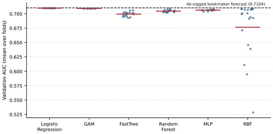
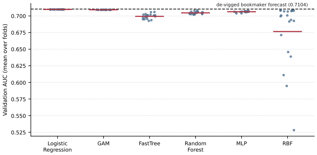
The sensitivity of the results to the hyperparameter settings is reported in Figure 3. For each of the six classifiers, every configuration drawn in the random search is plotted against the validation AUC it obtained on the expanding-window folds described in the experimental settings subsection, together with the de-vigged market forecast evaluated on the same folds. Two features are apparent. Five of the six classifiers show limited sensitivity over the sampled ranges, the widest of them varying by no more than 0.014 in validation AUC, whereas the RBF varies by 0.181 and is therefore strongly dependent on its kernel scale. Nevertheless, the best configuration attained by each classifier lies in a narrow band between 0.7061 and 0.7098, so the choice of configuration within these ranges does not change which predictors are comparable with which. The whole of that band lies below the market reference, which no configuration of any classifier reaches.

Figure 3. Hyperparameter sensitivity in the Home Win market. Each point is one of the twenty configurations drawn for a classifier, scored by three-fold expanding-window validation inside the training set; the horizontal bar is the mean of the classifier and the dashed line is the de-vigged bookmaker forecast evaluated on the same folds. The search was carried out on the most recent 50,000 matches of the training set and the test set was not used at any stage.

4. Conclusions

This study presented a unified benchmarking study for football match outcome classification, evaluating six classifiers—Logistic Regression, GAM, FastTree, RF, RBF and MLP—on a large-scale dataset of 225,474 matches spanning 2018–2026. Under strictly uniform experimental conditions, the six classifiers performed almost identically. In the Home Win market error ranged from 34.50% to 34.73% and macro-averaged Precision from 64.83% to 65.16%; in the Away Win market from 27.83% to 27.98% and from 68.05% to 68.46%, respectively. In both markets, the marginal bootstrap intervals overlap substantially, and the small differences between the point estimates are not interpreted as evidence of a ranking. What does separate the predictors is the comparison with the two reference rows: every model improves clearly on the majority-class baseline, and every model coincides with the de-vigged bookmaker forecast to within a small fraction of a percentage point.

These results indicate that under a common experimental protocol, the choice among six established classifiers has a smaller effect on predictive performance than the information contained in the feature set: without odds-based inputs, all six classifiers span only 0.08 accuracy points, and 0.27 points when the odds are included. When market prices are included among the inputs, every model reproduces the bookmaker forecast; when market prices are excluded, the models recover approximately half of the distance from a trivial baseline to the market (43.4% to 48.0% against 51.9% for the market). This is consistent with earlier evidence that odds-setters are competitive forecasters in their own right.

Several limitations should be stated. First, no model improves upon the de-vigged bookmaker forecast on any proper scoring rule; the GAM attains a small advantage in accuracy, which is not a proper scoring rule and which is not accompanied by any improvement in logarithmic loss, Brier score or the RPS, so the comparison with the market should be read as a benchmark rather than as evidence of practical advantage. That advantage is the only statistically distinguishable improvement over the market reported anywhere in this study, and it corresponds to about 65 additional correct predictions out of 75,495. Second, only a single pre-match odds snapshot from one provider is available, so neither the movement of odds between opening and closing nor the dispersion of prices across providers—the two signals most often associated with market inefficiency—can be examined. Third, player-level and lineup information is not available, which restricts the feature space to team-level aggregates. Fourth, the draw outcome is poorly predicted both by the models and by the market (AUC 0.584), and single-threshold measures are uninformative for it. Fifth, historical features must be imputed for 22.4% of matches, mainly newly promoted teams and matches early in a season; the associated data-availability indicators carry measurable predictive signal, but that signal reflects the composition of the dataset rather than any footballing quantity, and a robustness check reported in the feature-importance subsection shows that removing them costs at most 0.22 accuracy points and leaves the conclusions unchanged. Sixth, the analysis is confined to the pooled dataset: per-competition modelling and cross-competition transfer were not examined and are left for future work. Finally, probability calibration is not addressed in this study: applying an isotonic or Platt correction to the model outputs and testing whether it improves the probabilistic scores reported above is left for future work.

We have not added recurrent or attention-based baselines, and the reason is empirical rather than practical. The feature space consists of team-level attributes summarised per match, with no sequential or relational structure of the kind these architectures exploit. As an additional diagnostic, a Logistic Regression was fitted on the training set with the de-vigged market log-odds entered as a fixed offset, so that the remaining standardised features could only correct it, and the fitted correction was small. The convergence of six classifiers of very different flexibility, reported above, points to the information in the available features rather than model capacity as the principal constraint, and therefore provides limited empirical motivation for applying substantially more complex architectures to the same inputs. We present this as an indication rather than a proof: six converging classifiers and a small offset correction constitute strong empirical evidence, not a demonstration that no more expressive architecture could help.

Future work will extend the analysis to competitions modelled individually, to the question of distribution shift between them, and to competitions beyond those currently available, and will investigate whether league-aware feature engineering or transfer-learning strategies are of use when a model is confined to a single, smaller competition. Two directions appear particularly promising: the use of odds movement and cross-provider price dispersion, which would allow the market benchmark to be tested rather than merely matched, and the incorporation of sequential match-event data, for which recurrent or attention-based architectures would be appropriate.

References

- Kashinath, K.; Mustafa, M.; Albert, A.; Wu, J.; Jiang, C.; Esmaeilzadeh, S.; Azizzadenesheli, K.; Wang, R.; Chattopadhyay, A.; Singh, A.; et al. Physics-informed machine learning: Case studies for weather and climate modelling. Philos. Trans. R. Soc. A 2021, 379, 20200093. [Google Scholar] [CrossRef] [Scilit] [PubMed]
- Viquar, M.; Basak, S.; Dasgupta, A.; Agrawal, S.; Saha, S. Machine learning in astronomy: A case study in quasar-star classification. In Emerging Technologies in Data Mining and Information Security: Proceedings of IEMIS 2018; Springer: Berlin/Heidelberg, Germany, 2019; Volume 3, pp. 827–836. [Google Scholar] [CrossRef] [Scilit]
- Luo, S.; Leung, A.P.; Hui, C.Y.; Li, K.L. An investigation on the factors affecting machine learning classifications in gamma-ray astronomy. Mon. Not. R. Astron. Soc. 2020, 492, 5377–5390. [Google Scholar] [CrossRef] [Scilit]
- Meuwly, M. Machine learning for chemical reactions. Chem. Rev. 2021, 121, 10218–10239. [Google Scholar] [CrossRef] [Scilit] [PubMed]
- Aguiar, J.A.; Gong, M.L.; Tasdizen, T. Crystallographic prediction from diffraction and chemistry data for higher throughput classification using machine learning. Comput. Mater. Sci. 2020, 173, 109409. [Google Scholar] [CrossRef] [Scilit]
- Raissi, M.; Karniadakis, G.E. Hidden physics models: Machine learning of nonlinear partial differential equations. J. Comput. Phys. 2018, 357, 125–141. [Google Scholar] [CrossRef] [Scilit]
- Yadav, S.S.; Jadhav, S.M. Deep convolutional neural network based medical image classification for disease diagnosis. J. Big Data 2019, 6, 113. [Google Scholar] [CrossRef] [Scilit]
- Li, Q.; Weng, L.; Ding, X. A Novel Neural Network-Based Method for Medical Text Classification. Future Internet 2019, 11, 255. [Google Scholar] [CrossRef] [Scilit]
- Athey, S. The impact of machine learning on economics. In The Economics of Artificial Intelligence: An Agenda; University of Chicago Press: Chicago, IL, USA, 2018; pp. 507–547. [Google Scholar] [CrossRef] [Scilit]
- Hafezi, R.; Shahrabi, J.; Hadavandi, E. A bat-neural network multi-agent system (BNNMAS) for stock price prediction: Case study of DAX stock price. Appl. Soft Comput. 2015, 29, 196–210. [Google Scholar] [CrossRef] [Scilit]
- Ghai, D.; Tripathi, S.L.; Saxena, S.; Chanda, M.; Alazab, M. (Eds.) Machine Learning Algorithms for Signal and Image Processing; John Wiley & Sons: Hoboken, NJ, USA, 2022. [Google Scholar] [CrossRef] [Scilit]
- Ahmed, N.K.; Atiya, A.F.; Gayar, N.E.; El-Shishiny, H. An empirical comparison of machine learning models for time series forecasting. Econom. Rev. 2010, 29, 594–621. [Google Scholar] [CrossRef] [Scilit]
- Zou, J.; Han, Y.; So, S.S. Overview of artificial neural networks. Artif. Neural Netw. Methods Appl. 2009, 458, 14–22. [Google Scholar] [CrossRef] [Scilit] [PubMed]
- Abiodun, O.I.; Jantan, A.; Omolara, A.E.; Dada, K.V.; Mohamed, N.A.; Arshad, H. State-of-the-art in artificial neural network applications: A survey. Heliyon 2018, 4, e00938. [Google Scholar] [CrossRef] [Scilit] [PubMed]
- De Ville, B. Decision trees. WIREs Comput. Stat. 2013, 5, 448–455. [Google Scholar] [CrossRef] [Scilit]
- Kotsiantis, S.B. Decision trees: A recent overview. Artif. Intell. Rev. 2013, 39, 261–283. [Google Scholar] [CrossRef] [Scilit]
- Pisner, D.A.; Schnyer, D.M. Support vector machine. In Machine Learning; Academic Press: Cambridge, MA, USA, 2020; pp. 101–121. [Google Scholar] [CrossRef] [Scilit]
- Valkenborg, D.; Rousseau, A.J.; Geubbelmans, M.; Burzykowski, T. Support vector machines. Am. J. Orthod. Dentofac. Orthop. 2023, 164, 754–757. [Google Scholar] [CrossRef] [Scilit] [PubMed]
- Forrest, D.; Goddard, J.; Simmons, R. Odds-setters as forecasters: The case of English football. Int. J. Forecast. 2005, 21, 551–564. [Google Scholar] [CrossRef] [Scilit]
- Dixon, M.J.; Coles, S.G. Modelling association football scores and inefficiencies in the football betting market. J. R. Stat. Soc. Ser. C 1997, 46, 265–280. [Google Scholar] [CrossRef] [Scilit]
- Kliger, D.; Mugerman, Y.; Rooz, R. Eponymy family firms and optimistic forecasts. Financ. Res. Lett. 2025, 85, 108032. [Google Scholar] [CrossRef] [Scilit]
- Hvattum, L.M.; Arntzen, H. Using ELO ratings for match result prediction in association football. Int. J. Forecast. 2010, 26, 460–470. [Google Scholar] [CrossRef] [Scilit]
- Marcot, B.G.; Penman, T.D. Advances in Bayesian network modelling: Integration of modelling technologies. Environ. Model. Softw. 2019, 111, 386–393. [Google Scholar] [CrossRef] [Scilit]
- Owramipur, F.; Eskandarian, P.; Mozneb, F.S. Football result prediction with Bayesian network in Spanish League-Barcelona team. Int. J. Comput. Theory Eng. 2013, 5, 812. [Google Scholar] [CrossRef] [Scilit]
- Stoltzfus, J.C. Logistic regression: A brief primer. Acad. Emerg. Med. 2011, 18, 1099–1104. [Google Scholar] [CrossRef] [Scilit] [PubMed]
- Prasetio, D.; Harlili, D. Predicting football match results with logistic regression. In Proceedings of the International Conference On Advanced Informatics: Concepts, Theory and Application (ICAICTA), Penang, Malaysia, 16–19 August 2016; pp. 1–5. [Google Scholar] [CrossRef] [Scilit]
- Martins, R.G.; Martins, A.S.; Neves, L.A.; Lima, L.V.; Flores, E.L.; do Nascimento, M.Z. Exploring polynomial classifier to predict match results in football championships. Expert Syst. Appl. 2017, 83, 79–93. [Google Scholar] [CrossRef] [Scilit]
- Schauberger, G.; Groll, A. Predicting matches in international football tournaments with random forests. Stat. Model. 2018, 18, 460–482. [Google Scholar] [CrossRef] [Scilit]
- Danisik, N.; Lacko, P.; Farkas, M. Football match prediction using players attributes. In 2018 World Symposium on Digital Intelligence for Systems and Machines (DISA); IEEE: New York, NY, USA, 2018; pp. 201–206. [Google Scholar] [CrossRef] [Scilit]
- Constantinou, A.C. Dolores: A model that predicts football match outcomes from all over the world. Mach. Learn. 2019, 108, 49–75. [Google Scholar] [CrossRef] [Scilit]
- Natekin, A.; Knoll, A. Gradient boosting machines, a tutorial. Front. Neurorobotics 2013, 7, 63623. [Google Scholar] [CrossRef] [Scilit] [PubMed]
- Baboota, R.; Kaur, H. Predictive analysis and modelling football results using machine learning approach for English Premier League. Int. J. Forecast. 2019, 35, 741–755. [Google Scholar] [CrossRef] [Scilit]
- Rahman, M.A. A deep learning framework for football match prediction. SN Appl. Sci. 2020, 2, 165. [Google Scholar] [CrossRef] [Scilit]
- Clarke, S.R.; Kovalchik, S.A.; Ingram, M. Adjusting Bookmaker’s Odds to Allow for Overround. Am. J. Sports Sci. 2017, 5, 45–49. [Google Scholar] [CrossRef] [Scilit]
- Wood, S.N. Generalized Additive Models: An Introduction with R, 2nd ed.; Chapman and Hall/CRC: Boca Raton, FL, USA, 2017. [Google Scholar] [CrossRef] [Scilit]
- Friedman, J.H. Greedy function approximation: A gradient boosting machine. Ann. Stat. 2001, 29, 1189–1232. [Google Scholar] [CrossRef] [Scilit]
- Liaw, A.; Wiener, M. Classification and regression by random Forest. R News 2002, 2, 18–22. [Google Scholar]
- Rahimi, A.; Recht, B. Random features for large-scale kernel machines. In Advances in Neural Information Processing Systems 20; NeurIPS: San Diego, CA, USA, 2008; pp. 1177–1184. [Google Scholar]
- Efron, B.; Tibshirani, R.J. An Introduction to the Bootstrap; Chapman & Hall/CRC: Boca Raton, FL, USA, 1993. [Google Scholar]
- Gneiting, T.; Raftery, A.E. Strictly proper scoring rules, prediction, and estimation. J. Am. Stat. Assoc. 2007, 102, 359–378. [Google Scholar] [CrossRef] [Scilit]
- Constantinou, A.C.; Fenton, N.E. Solving the problem of inadequate scoring rules for assessing probabilistic football forecast models. J. Quant. Anal. Sports 2012, 8. [Google Scholar] [CrossRef] [Scilit]
- Wheatcroft, E. Evaluating probabilistic forecasts of football matches: The case against the ranked probability score. J. Quant. Anal. Sports 2021, 17, 273–287. [Google Scholar] [CrossRef] [Scilit]
Disclaimer/Publisher’s Note: The statements, opinions and data contained in all publications are solely those of the individual author(s) and contributor(s) and not of MDPI and/or the editor(s). MDPI and/or the editor(s) disclaim responsibility for any injury to people or property resulting from any ideas, methods, instructions or products referred to in the content. |
© 2026 by the authors. Licensee MDPI, Basel, Switzerland. This article is an open access article distributed under the terms and conditions of the Creative Commons Attribution (CC BY) license.