A Marchuk’s Model Analysis by Proposed Decomposition Theorem

Abstract

Taking the Singularly Perturbed System (SPS) as a model of ODE system separation into fast and slow subsystems by an arbitrarily small parameter, we state and prove a theorem on the decomposition of an Ordinary Differential Equations (ODE) system without the aforementioned arbitrarily small parameter. In accordance with the proven theorem, we implemented an algorithm to decompose an ODE system into fast and slow subsystems by coordinate transformation. A similar algorithm is called the Singular Perturbed Vector Field (SPVF) algorithm; however, it is not justified by any stated theorem. Since we have not found any theorem to propose a similar ODE decomposition in the literature, we have tried to fill the gap with our theorem and algorithm explanations through examples. Finally, we propose our concept on Marchuk’s infectious diseases model, which allows a different analysis of the original Marchuk’s ODE system with delay.

1. Introduction

In biology, as in other fields of science, a change in one quantity depends on changes in several other quantities that are measured in the observed process. The fact that they affect each other forms the basis for creating mathematical models [1] in the form of ODE systems. In [2,3], we found an algorithm where the ODE system is decomposed into so-called fast and slow manifolds. Since a specific biological process involves many factors [4], some of them accelerate the progression of a disease, while the others slow it down. Therefore, we decided to improve this algorithm, which, by changing the coordinates, splits the original ODE system into fast and slow subsystems.

If changes are observed only in time, biological processes are modeled by ODE systems describing time derivatives of state variables. Applications of ODE-based modeling to chemo-immunotherapy treatment design have been explored in [5]. Now, we write the system in the generally accepted form and refer to it in our subsequent calculations.

$$\begin{array}{ccc}\hfill {\displaystyle \frac{dz}{dt}}& =& \Phi \left(z\right)\hfill \end{array}$$

(1)

$$\begin{array}{ccc}\hfill z(t=0)& =& z_0={(z_{01},\dots ,z_{0n})}^T\in \Omega \subseteq {\mathbb{R}}^n,\hfill \end{array}$$

(2)

where $z_0$ is an arbitrary point.

The classical existence–uniqueness result is due to Picard [6] (see Tome II, p. 301) and [7] (see Gallica scan) for the original treatments, and [8] or [9] for modern expositions.

We are primarily inspired by [2,10], which transformed an ODE system into an SPS by a coordinate change. Although the algorithms in [2,10] are clearly stated, in the mentioned articles, we did not come across a proven theorem that would support the algorithms. Our intention is to fill this gap with a proof of a theorem that supports the algorithms we implemented. For the first time, we define an SPS, as defined in [11].

Definition 1.

An SPS is written in the form $0<ϵ\ll 1$ as follows:

$$\begin{array}{ccc}\hfill {\displaystyle \frac{dx}{dt}}& =& {\displaystyle \frac{1}{ϵ}}F(x,y,ϵ)\hfill \end{array}$$

(3)

$$\begin{array}{ccc}\hfill {\displaystyle \frac{dy}{dt}}& =& G(x,y,ϵ).\hfill \end{array}$$

(4)

If $dt=ϵd\tau$, then:

$$\begin{array}{ccc}\hfill {\displaystyle \frac{dx}{d\tau }}& =& F(x,y,ϵ)\hfill \end{array}$$

(5)

$$\begin{array}{ccc}\hfill {\displaystyle \frac{dy}{d\tau }}& =& ϵG(x,y,ϵ).\hfill \end{array}$$

(6)

Here, $x\in {\mathbb{R}}^{n_f}$, $y\in {\mathbb{R}}^{n_s}$, and $n_f+n_s=n$. Smooth vector mappings $F(x,y,ϵ),G(x,y,ϵ):\Omega \to {\mathbb{R}}^{n_f},{\mathbb{R}}^{n_s}$ satisfy $F(x,y,ϵ),G(x,y,ϵ)\sim O\left(1\right)$.

In the next section, we give the theoretical basis for the algorithms in the following section. $F(x,y,ϵ),G(x,y,ϵ)\sim O\left(1\right)$ means that when $ϵ\to 0$, the functions $F(x,y,ϵ)$ and $G(x,y,ϵ)$ do not tend to 0 or blow up. Instead, there exist ${ϵ}_0$ and C, such that if $0<ϵ<{ϵ}_0$, then $F(x,y,ϵ),G(x,y,ϵ)\le C$.

2. Materials and Methods

As $\{x,y,ϵ\}$ approach certain values or infinity, the functions’ outputs $F(x,y,ϵ)$ and $G(x,y,ϵ)$ do not grow infinitely large. Instead, they are always less than some constant value. The singularity in Definition 1 is achieved when the parameter $ϵ$ tends to 0.

Although [2] is dedicated to the decomposition of ODE systems into slow and fast manifolds, the manifolds themselves are not formally defined. We did not find a formal definition, even in [10]. In the remark that follows, we try to justify the fast and slow manifold terminology mentioned in [10], on page 30.

Remark 1.

Reference [10] does not give an initial condition, so here we use:

$$(x\left(0\right),y\left(0\right))=(x_0,y_0).$$

(7)

The initial condition is important now, because if $F(x,y,ϵ)=0$, then we have the system

$$\begin{array}{ccc}\hfill {\displaystyle \frac{dx}{dt}}& =& 0\hfill \end{array}$$

(8)

$$\begin{array}{ccc}\hfill {\displaystyle \frac{dy}{dt}}& =& G(x,y,ϵ).\hfill \end{array}$$

(9)

The first equation is then trivial to solve:

$$x\left(t\right)=C,$$

(10)

and from (7), we have $C=x_0$, so $x\left(t\right)=x_0$ for all t of the interval considered. After that, we solve the subsystem

$${\displaystyle \frac{dy}{dt}}=G(x_0,y,ϵ),$$

(11)

and obtain the slow solution as a curve on the manifold $F(x,y,ϵ)=0$. By the definition in [10] (below their Equation (6)), the manifold $F(x,y,ϵ)=0$ is called the slow manifold.

On the other hand, if $G(x,y,ϵ)=0$, then systems (3) and (4) turn into system

$$\begin{array}{ccc}\hfill {\displaystyle \frac{dx}{dt}}& =& {\displaystyle \frac{1}{ϵ}}F(x,y,ϵ)\hfill \end{array}$$

(12)

$$\begin{array}{ccc}\hfill {\displaystyle \frac{dy}{dt}}& =& 0.\hfill \end{array}$$

(13)

According to (12) and (7), we have $y\left(t\right)=y_0$ for the interval $t\in [-t_0,t_0]$. Therefore, we solve the following problems

$${\displaystyle \frac{dx}{dt}}={\displaystyle \frac{1}{ϵ}}F(x,y_0,ϵ),$$

(14)

and obtain a fast solution as a curve on the manifold $G(x,y,ϵ)=0$. In [10] (see again the text in [10] below the equation noted there by (6)), by analogy, $G(x,y,ϵ)=0$ is called the fast manifold of the system (3) and (4).

Although [2] was published in a reputable, highly ranked journal, we did not find a proven theorem that justifies the algorithm for decomposing a three-dimensional ODE system into fast and slow subsystems by changing coordinates. The standard coordinates were transformed by the basis consisting of randomly selected matrix eigenvectors using an unjustified algorithm.

In the following, we prove a theorem to justify a decomposition algorithm that turns a system (1) into fast and slow subsystems alike, (3) and (4), but without the value $ϵ$ separating the fast and slow subsystems in Definition 1.

Theorem 1.

For any ODE system (1), there exist vector subspaces $L_f,L_s\subset {\mathbb{R}}^n$, such that $L_f\oplus L_s={\mathbb{R}}^n$. Furthermore, for the projections $P{r}_s\left({\mathbb{R}}^n\right):{\mathbb{R}}^n\to L_s$ and $P{r}_f:{\mathbb{R}}^n\to L_f$, the next inequality holds

$$\underset{z\in {\mathbb{R}}^n}{sup}|P{r}_s\Phi \left(z\right)|\le \underset{z\in {\mathbb{R}}^n}{inf}|P{r}_f\Phi \left(z\right)|.$$

(15)

Proof. 

Denote the vector field in (1) by the column vector $\Phi \left(z\right)={({\Phi }_1\left(z\right),\dots ,{\Phi }_n\left(z\right))}^T$. Choose n linearly independent points

$$\{z_1,\dots ,z_n\}\subset \Omega ,$$

(16)

such that the vector field values $\{\Phi \left(z_1\right),\dots ,\Phi \left(z_n\right)\}$ are independent too, and create a matrix with these vector field values as the matrix columns:

$$T=\left[{\Phi }_i\left(z_j\right)\right]=\left[\begin{array}{cccc}{\Phi }_1\left(z_1\right)& {\Phi }_1\left(z_2\right)& \dots & {\Phi }_1\left(z_n\right)\\ {\Phi }_2\left(z_1\right)& {\Phi }_2\left(z_2\right)& \dots & {\Phi }_2\left(z_n\right)\\ ⋮& ⋮& \ddots & ⋮\\ {\Phi }_n\left(z_1\right)& {\Phi }_n\left(z_2\right)& \dots & {\Phi }_n\left(z_n\right)\end{array}\right].$$

(17)

Let $T^T$ denote the transpose of T. Then, the product $T·T^T=T{T}^T$ is symmetric, since ${\left(T{T}^T\right)}^T=T{T}^T$. By the fundamental theorem of algebra, for the unit matrix $E=\left({\delta }_{ij}\right)$, the equation for $\lambda$ given by

$$det(T-\lambda E)=0$$

(18)

has n non-negative real roots. The roots ${\lambda }_i,i=1,\dots ,n$ are eigenvalues of $T{T}^T$ and we can sort them by increasing the value:

$${\lambda }_1\le {\lambda }_2\le \cdots \le {\lambda }_n.$$

(19)

After finding the maximum gap:

$$\underset{i=1,2,\dots ,n-1}{max}{\displaystyle \frac{{\lambda }_{i+1}}{{\lambda }_i}}={\displaystyle \frac{{\lambda }_{n_s+1}}{{\lambda }_{n_s}}},$$

(20)

the eigenvalue sequence (19) is separated into $n_s$ slow, and $n_f=n-n_s$ fast eigenvalues:

$${\lambda }_1\le \cdots \le {\lambda }_{n_s}\le {\lambda }_{n_s+1}\le \cdots \le {\lambda }_n.$$

(21)

We denote the slow eigenvectors by ${\mathbf{y}}_i$ iff $T{T}^T{\mathbf{y}}_i={\lambda }_i{\mathbf{y}}_i$ for $i=1,2,\dots ,n_s$, and we denote the fast eigenvectors by ${\mathbf{x}}_i$, iff $T{T}^T{\mathbf{x}}_i={\lambda }_{n_s+i}{\mathbf{x}}_i$ for $i=1,2,\dots ,n_f$. Without loss of generality, we assume that all eigenvectors are unit vectors. Since $T{T}^T$ is symmetric, the eigenvectors corresponding to different eigenvalues in (21) are mutually orthogonal, and we have the new orthonormal basis for the tangent bundle:

$$\{{\mathbf{x}}_1,\dots ,{\mathbf{x}}_{n_f},{\mathbf{y}}_1,\dots ,{\mathbf{y}}_{n_s}\}.$$

(22)

For eigenvectors belonging to the same eigenvalue and not necessarily perpendicular to each other, there is always an orthonormal basis of that eigen-subspace. Without loss of generality, we assume that all eigenvalues are different. Moreover, identical eigenvalues do not occur by chance. Finally, we define the fast and slow subspaces spanned by the eigenvectors corresponding to (21):

$$L_f=span\left[\{{\mathbf{x}}_1,\dots ,{\mathbf{x}}_{n_f}\}\right]\mathrm{and}{L}_s=span\left[\{{\mathbf{y}}_1,\dots ,{\mathbf{y}}_{n_s}\}\right].$$

(23)

After we have defined $L_f$ and $L_s$, it remains to prove inequality (15). By orthonormal eigenvectors from (22), we diagonalize the matrix $T{T}^T$:

$$T{T}^T=\left[\begin{array}{cc}\mathbf{x}& \mathbf{y}\end{array}\right]\left[\begin{array}{cc}{\lambda }_f& 0\\ 0& {\lambda }_s\end{array}\right]{\left[\begin{array}{cc}\mathbf{x}& \mathbf{y}\end{array}\right]}^T,$$

(24)

since $T{T}^T$ is symmetric, $\left[\begin{array}{cc}\mathbf{x}& \mathbf{y}\end{array}\right]$ is orthonormal and $\left[\begin{array}{cc}\mathbf{x}& \mathbf{y}\end{array}\right]\left[\begin{array}{c}\mathbf{x}\\ \mathbf{y}\end{array}\right]=E$.

We use the abbreviations $\mathbf{x}={\left[\begin{array}{ccc}{\mathbf{x}}_1& \cdots & {\mathbf{x}}_{n_f}\end{array}\right]}^T$ and $\mathbf{y}={\left[\begin{array}{ccc}{\mathbf{y}}_1& \cdots & {\mathbf{y}}_{n_s}\end{array}\right]}^T$ for the columns consisting of the fast and slow vector coordinates given below in the rows of (27). Also, we use abbreviations for diagonal block matrices in (24) obtained from so-called slow and fast eigenvalues from (21):

$${\lambda }_s=\left[\begin{array}{cccc}{\lambda }_1& 0& \cdots & 0\\ 0& 0& \ddots & 0\\ ⋮& ⋮& \ddots & 0\\ 0& 0& \cdots & {\lambda }_{n_s}\end{array}\right],{\lambda }_f=\left[\begin{array}{cccc}{\lambda }_{n_s+1}& 0& \cdots & 0\\ 0& 0& \ddots & 0\\ ⋮& ⋮& \ddots & 0\\ 0& 0& \cdots & {\lambda }_n\end{array}\right].$$

(25)

To prove the inequality (15), we change the standard tangent bundle coordinate basis:

$$\left\{{\displaystyle \frac{d{z}_1}{dt},\frac{d{z}_2}{dt},\dots ,\frac{d{z}_n}{dt}}\right\}$$

(26)

into basis (22). In the base (26), the vectors from (22) are presented as follows:

$$\begin{array}{ll}{\mathbf{x}}_1& =\hspace{1em}{x}_{11}{\displaystyle \frac{d{z}_1}{dt}}+x_{12}{\displaystyle \frac{d{z}_2}{dt}}+\cdots +x_{1n}{\displaystyle \frac{d{z}_n}{dt}}\\ {\mathbf{x}}_2& =\hspace{1em}{x}_{21}{\displaystyle \frac{d{z}_2}{dt}}+x_{22}{\displaystyle \frac{d{z}_2}{dt}}+\cdots +x_{2n}{\displaystyle \frac{d{z}_n}{dt}}\\ & ⋮\\ {\mathbf{x}}_{n_f}& =\hspace{1em}{x}_{n_{f}1}{\displaystyle \frac{d{z}_1}{dt}}+x_{n_{f}2}{\displaystyle \frac{d{z}_2}{dt}}+\cdots +x_{n_{f}n}{\displaystyle \frac{d{z}_n}{dt}}\\ {\mathbf{y}}_1& =\hspace{1em}{y}_{11}{\displaystyle \frac{d{z}_1}{dt}}+y_{12}{\displaystyle \frac{d{z}_2}{dt}}+\cdots +y_{1n}{\displaystyle \frac{d{z}_n}{dt}}\\ {\mathbf{y}}_2& =\hspace{1em}{y}_{21}{\displaystyle \frac{d{z}_2}{dt}}+y_{22}{\displaystyle \frac{d{z}_2}{dt}}+\cdots +y_{2n}{\displaystyle \frac{d{z}_n}{dt}}\\ & ⋮\\ {\mathbf{y}}_{n_s}& =\hspace{1em}{y}_{n_{s}1}{\displaystyle \frac{d{z}_1}{dt}}+y_{n_{s}2}{\displaystyle \frac{d{z}_2}{dt}}+\cdots +y_{n_{s}n}{\displaystyle \frac{d{z}_n}{dt}}\end{array}$$

(27)

Substituting (1) into (27), we obtain a new ODE system with the same solution as (1), but in the new orthonormal coordinates. Moreover, the new system obtained from (27) by substitution (1) is separated into two subsystems. The first $n_f$ equations make up the fast subsystem, and the second $n_s$ equations make up the slow subsystem. In matrix form, (27) is written by natural notation for mapped vectors:

$$\left[\begin{array}{c}\mathbf{x}\\ \mathbf{y}\end{array}\right]=A{\displaystyle \frac{dz}{dt}}.$$

(28)

Because the matrix $T{T}^T$ is regular, the matrix A with constant members is regular also. Changing the coordinates in ODE domain $\Omega \subseteq {\mathbb{R}}^n$ by

$$\left[\begin{array}{c}x\\ y\end{array}\right]=Az,$$

(29)

we obtain coordinate changing (30) in the tangent bundle of $\Omega$ by deriving (29):

$$\left[\begin{array}{c}{\displaystyle \frac{dx}{dt}}\\ {\displaystyle \frac{dy}{dt}}\end{array}\right]=A{\displaystyle \frac{dz}{dt}}.$$

(30)

Formula (30) presents (28) with a natural notation:

$$\begin{array}{cc}\hfill \mathbf{x}& ={\displaystyle \frac{dx}{dt}}\hfill \\ \hfill \mathbf{y}& ={\displaystyle \frac{dy}{dt}}.\hfill \end{array}$$

(31)

From (27), we obtain $A={\left[\begin{array}{cc}\mathbf{x}& \mathbf{y}\end{array}\right]}^T$. If the solution curve $z\left(t\right)$ satisfies (1), then (30) becomes:

$$\left[\begin{array}{c}{\displaystyle \frac{dx}{dt}}\\ {\displaystyle \frac{dy}{dt}}\end{array}\right]={\left[\begin{array}{cc}\mathbf{x}& \mathbf{y}\end{array}\right]}^T\Phi \left(z\right),$$

(32)

with a constant matrix $\left[\begin{array}{cc}\mathbf{x}& \mathbf{y}\end{array}\right]$ from (27), and regularity in (29) guarantees that the system (1) is equivalent to the system:

$$\left[\begin{array}{c}{\displaystyle \frac{dx}{dt}}\\ {\displaystyle \frac{dy}{dt}}\end{array}\right]={\left[\begin{array}{cc}\mathbf{x}& \mathbf{y}\end{array}\right]}^T\Phi \left(A^{-1}\left[\begin{array}{c}x\\ y\end{array}\right]\right).$$

(33)

We construct the projections noted in (15) by applying the matrix $T{T}^T$ from (17) and with the matrix A given in (29). Acting on both sides in (33) by $T{T}^T$, we have

$$T{T}^T\left(\begin{array}{c}{\displaystyle \frac{dx}{dt}}\\ {\displaystyle \frac{dy}{dt}}\end{array}\right)=T{\left[\begin{array}{cc}\mathbf{x}& \mathbf{y}\end{array}\right]}^T\Phi \left(A^{-1}\left(\begin{array}{c}x\\ y\end{array}\right)\right).$$

(34)

When the standard basis in the $\Omega$ tangent bundle is changed by (22), then the vectors in (22) become unit vectors in the bundle, and we claim:

$$\left[\begin{array}{cc}\mathbf{x}& \mathbf{y}\end{array}\right]={\left[\begin{array}{cc}\mathbf{x}& \mathbf{y}\end{array}\right]}^{-1}={\left[\begin{array}{cc}\mathbf{x}& \mathbf{y}\end{array}\right]}^T=E.$$

(35)

Thus, the matrix $T{T}^T$ from (24) now reads:

$$T{T}^T=\left[\begin{array}{cc}{\lambda }_f& 0\\ 0& {\lambda }_s\end{array}\right],$$

(36)

and Equation (34) turns out to be

$$\left[\begin{array}{cc}{\lambda }_f& 0\\ 0& {\lambda }_s\end{array}\right]\left(\begin{array}{c}{\displaystyle \frac{dx}{dt}}\\ {\displaystyle \frac{dy}{dt}}\end{array}\right)=\left[\begin{array}{cc}{\lambda }_f& 0\\ 0& {\lambda }_s\end{array}\right]\Phi \left(A^{-1}\left(\begin{array}{c}x\\ y\end{array}\right)\right).$$

(37)

Now, we define projections from (15) as the right-hand side (RHS) in (37):

$$\begin{array}{ll}P{r}_f\Phi \left(A^{-1}\left(\begin{array}{c}x\\ y\end{array}\right)\right)& =\left[\begin{array}{cc}{\lambda }_f& 0\\ 0& 0\end{array}\right]\Phi \left(A^{-1}\right(\begin{array}{c}x\\ y\end{array}\left)\right)\\ P{r}_s\Phi \left(A^{-1}\right(\begin{array}{c}x\\ y\end{array}\left)\right)& =\left[\begin{array}{cc}0& 0\\ 0& {\lambda }_s\end{array}\right]\Phi \left(A^{-1}\right(\begin{array}{c}x\\ y\end{array}\left)\right).\end{array}$$

(38)

Respecting the changing (29) in $\Omega$, in old coordinates, we claim:

$$\begin{array}{cc}\hfill P{r}_f\Phi \left(z\right)& =\left[\begin{array}{cc}{\lambda }_f& 0\\ 0& 0\end{array}\right]\Phi \left(z\right)\hfill \\ \hfill P{r}_s\Phi \left(z\right)& =\left[\begin{array}{cc}0& 0\\ 0& {\lambda }_s\end{array}\right]\Phi \left(z\right).\hfill \end{array}$$

(39)

Inequality (15) now slides from (21), because (21) ensures

$$|{\lambda }_s{|}^2=\sum _{i=1}^{n_s}|{\lambda }_i{|}^2\le \sum _{i=1}^{n_f}|{\lambda }_{n_s+}{i|}^2={|{\lambda }_f|}^2.$$

(40)

Given that ${\lambda }_s$ and ${\lambda }_f$ are a diagonal constant matrix, from (39), we claim

$$\left|P{r}_s\Phi \left(z\right)\right|=\left|{\lambda }_s\right|·\left|\Phi \left(z\right)\right|\le \left|{\lambda }_f\right|·\left|\Phi \left(z\right)\right|=\left|P{r}_f\Phi \left(z\right)\right|,$$

(41)

since the new base vectors in (22) are orthonormal. □

We prove a decomposition without valuating it. Theorem 1 justifies an algorithm similar to what is carried out in [2]. Decomposition depends on initial points selected in (16), so in Section 3, the algorithm is carried out with comments that explain the algorithm’s steps for selecting initial points. Furthermore, we draw out the fast and slow manifolds in both old and new coordinates. As a consequence of Theorem 1, we have the following theorem.

Theorem 2.

For any ODE system (1), there exist vector fields $F:\Omega \to L_f$ and $G:\Omega \to L_s$, such that for the system given by

$$\begin{array}{ccc}\hfill {\displaystyle \frac{dx}{dt}}& =& F(x,y)\hfill \end{array}$$

(42)

$$\begin{array}{ccc}\hfill {\displaystyle \frac{dy}{dt}}& =& G(x,y),\hfill \end{array}$$

(43)

the next inequality holds:

$$\left|F\right(x,y\left)\right|\ge \left|G\right(x,y\left)\right|.$$

(44)

Proof. 

According to (29), we define the vector fields of (39) as follows.

$$\begin{array}{cc}\hfill F(x,y)& =\left[\begin{array}{cc}{\lambda }_x& 0\\ 0& 0\end{array}\right]\Phi \left(A^{-1}\right(\begin{array}{c}x\\ y\end{array}\left)\right)\hfill \\ \hfill G(x,y)& =\left[\begin{array}{cc}0& 0\\ 0& {\lambda }_y\end{array}\right]\Phi \left(A^{-1}\left(\begin{array}{c}x\\ y\end{array}\right)\right).\hfill \end{array}$$

(45)

The inequality slides from proven (15). □

In the next remark, we relate the new coordinates’ decomposed system given in (33) with the system given in Definition 1 by (3) and (4).

Remark 2.

According to Theorem 1, from the ODE system (1), we obtain system (27). After substituting the right-hand sides from (1) and changing the coordinates by (29), in (27), the first equations $n_f$ make up the fast subsystem and the other equations $n_s$ make up the slow subsystem. In the SPS, the fast subsystem (3) and slow subsystem (4) are separated by $ϵ$. We conjecture, but do not prove, a possible relation between two separated systems:

$${\displaystyle ϵ=\frac{su{p}_{z\in {\mathbb{R}}^n}|P{r}_s\Phi \left(z\right)|}{{inf}_{z\in {\mathbb{R}}^n}|P{r}_f\Phi \left(z\right)|}.}$$

(46)

In the next sections, we present the procedures for transforming different ODE systems into SPSs by the coordinate change.

3. A Simple Method Presentation

In this section, we replace the coordinates with the eigenvalues of the matrix T that the author in [2] has defined identically (18). Using Theorem 1, we implement the strictly copied algorithm from [2], applying it manually to a simple two-dimensional problem. We plot the obtained slow and fast manifolds using the Geogebra [12].

Example 1.

For an ODE system given with

$$\begin{array}{cc}\hfill \frac{d{z}_1}{dt}& =z_1+z_2^2\hfill \\ \hfill \frac{d{z}_2}{dt}& =2z_1,\hfill \end{array}$$

(47)

construct fast and slow subsystems with corresponding fast and slow manifolds.

To carry out the procedure strictly according to [2], first we need to find a suitable independent points’ set (16) intended to obtain the maximal gap (20). Namely, Theorem 1 separates an ODE system from (1) to the system given by (3) and (4) with $ϵ=1$, in the case of any chosen (16).

In the next 10 steps, we find the base (16) where the gap (20) is largest. The steps given in [2] have not been interpreted at all, so here we give our steps interpretation.

• Regarding [2], first we randomly choose points in number N (much) greater than the domain space dimension. For $n=2$ in (47), we take $N=6\gg 2$ and randomly choose the points:

  $$\begin{array}{c}{z}^i\in \Gamma :=\left\{\right(\begin{array}{c}1\\ 0\end{array}),(\begin{array}{c}0\\ 1\end{array}),(\begin{array}{c}1\\ 2\end{array}),(\begin{array}{c}2\\ 2\end{array}),(\begin{array}{c}2\\ -3\end{array}),(\begin{array}{c}-2\\ 0\end{array}\left)\right\}.\end{array}$$
• According to (47), we calculate vector field values

  $$\begin{array}{c}\Phi \left(z^i\right)\in \left\{\right(\begin{array}{c}1\\ 2\end{array}),(\begin{array}{c}1\\ 0\end{array}),(\begin{array}{c}5\\ 2\end{array}),(\begin{array}{c}6\\ 4\end{array}),(\begin{array}{c}11\\ 4\end{array}),(\begin{array}{c}-2\\ -4\end{array}\left)\right\},\end{array}$$

  and their norms $|\Phi (z^i\left)\right|\in \{\sqrt{5},1,\sqrt{29},\sqrt{52},\sqrt{37},\sqrt{20}\}.$ As an example, for $z^1=\left(\begin{array}{c}1\\ 0\end{array}\right)$, and the vector field calculation $\Phi \left(\begin{array}{c}1\\ 0\end{array}\right)=\left(\begin{array}{c}{\Phi }_1\left(\begin{array}{c}1\\ 0\end{array}\right)\\ {\Phi }_2\left(\begin{array}{c}1\\ 0\end{array}\right)\end{array}\right)$, we have $\Phi \left(z^1\right)=\Phi \left(\begin{array}{c}1\\ 0\end{array}\right)=\left(\begin{array}{c}1\\ 2\end{array}\right)$ and $|\Phi (z^1\left)\right|=\sqrt{1^2+2^2}=\sqrt{5}.$
• To narrow down the number of randomly selected points from [1], we eliminate those that give vector field values less than the average. The average vector field $\overline{\Phi }$ is calculated by the formula:

  $$\overline{\Phi }=\frac{1}{N}\sum _{i=1}^N\Phi \left(z^i\right)=\frac{1}{6}\sum _{i=1}^6\left(\begin{array}{c}{\Phi }_1\left(z^i\right)\\ {\Phi }_2\left(z^i\right)\end{array}\right)=\frac{1}{6}\left(\begin{array}{c}22\\ 8\end{array}\right)$$

  (48)
• The norm of the average vector field from (48) is equal to

  $$|\overline{\Phi }|={\displaystyle \frac{1}{6}}\sqrt{{22}^2+8^2}=3.9$$
• From the set $\{\sqrt{5},1,\sqrt{29},\sqrt{52},\sqrt{37},\sqrt{20}\}$, we select the set:

  $${\Gamma }_{cs}=\{z^i\in \Gamma :|\Phi \left(z^i\right)|>|\Phi |,i=1,\dots ,N\}=\{\sqrt{29},\sqrt{52},\sqrt{37},\sqrt{20}\},$$

  and from $\Gamma$, the four initially chosen vectors rest:

  $${\Gamma }_{cs}=\{z^3,z^4,z^5,z^6\}=\left\{\right(\begin{array}{c}1\\ 2\end{array}),(\begin{array}{c}2\\ 2\end{array}),(\begin{array}{c}2\\ -3\end{array}),(\begin{array}{c}-2\\ 0\end{array}\left)\right\}.$$

  (49)
• We continue to further narrow down the set (49) by analyzing the volumes that the vectors from (49) already span. In this sense, we create a set of potential bases $\mathcal{B}=\{B_1,\dots ,B_m\},$ where $m=\left(\begin{array}{c}4\\ 2\end{array}\right)=6$, and we have six possible bases selected from (49): $B=\{B_1,B_2,B_3,B_4,B_5,B_6\}.$ Explicitly, the bases read
  $$B_1=\left\{\right(\begin{array}{c}1\\ 2\end{array}),(\begin{array}{c}2\\ 2\end{array}\left)\right\},B_2=\left\{\right(\begin{array}{c}2\\ -3\end{array}),(\begin{array}{c}-2\\ 0\end{array}\left)\right\},B_3=\left\{\right(\begin{array}{c}1\\ 2\end{array}),(\begin{array}{c}-2\\ 0\end{array}\left)\right\},$$

  $$B_4=\left\{\right(\begin{array}{c}1\\ 2\end{array}),(\begin{array}{c}2\\ -3\end{array}\left)\right\},B_5=\left\{\right(\begin{array}{c}2\\ -3\end{array}),(\begin{array}{c}2\\ 2\end{array}\left)\right\},B_6=\left\{\right(\begin{array}{c}2\\ 2\end{array}),(\begin{array}{c}-2\\ 0\end{array}\left)\right\},$$

  and give corresponding matrices:

  $$A_1=\left[\begin{array}{cc}1& 2\\ 2& 2\end{array}\right],A_2=\left[\begin{array}{cc}2& -2\\ -3& 0\end{array}\right],A_3=\left[\begin{array}{cc}1& -2\\ 2& 0\end{array}\right],$$

  $$A_4=\left[\begin{array}{cc}1& 2\\ 2& -3\end{array}\right],A_5=\left[\begin{array}{cc}2& 2\\ -3& 2\end{array}\right],A_6=\left[\begin{array}{cc}2& -2\\ 2& 0\end{array}\right].$$
  Calculating determinants from the matrices above, we obtain the vector span volumes.
• Calculating the determinants of suitable matrices gives the set of their absolute values:

  $$\left\{\right|det{A}_1|=2,|det{A}_2|=6,|det{A}_3|=4,|det{A}_4|=7,|det{A}_5|=10,|det{A}_6|=4\},$$

  and we narrow the set of bases in [6] by choosing those with volumes greater than the average. The average value of the absolute determinants’ $\overline{|detA|}$ is calculated as follows:

  $$\overline{|detA|}={\displaystyle \frac{1}{m}}\sum _{i=1}^m|det{A}_i|={\displaystyle \frac{1}{6}}(2+6+4+7+10+4)={\displaystyle \frac{33}{6}}=5.5.$$
  The bases corresponding to the matrices $A_i$ with $|det{A}_i|\ge \overline{|detA|}$ are as follows:

  $$B_2=\left\{\right(\begin{array}{c}2\\ -3\end{array}),(\begin{array}{c}-2\\ 0\end{array}\left)\right\},B_4=\left\{\right(\begin{array}{c}1\\ 2\end{array}),(\begin{array}{c}2\\ -3\end{array}\left)\right\},B_5=\left\{\right(\begin{array}{c}2\\ -3\end{array}),(\begin{array}{c}2\\ 2\end{array}\left)\right\}$$
  Next, we construct matrices according to (17) by calculating the vector field values for the vectors from bases $B_2,B_4$ and $B_5$.
• The vector field values’ matrix defined in (17) is now used to calculate the basis $B_2$:

  $$T_2=\left[\begin{array}{cc}\Phi \left(\begin{array}{c}2\\ -3\end{array}\right)& \Phi \left(\begin{array}{c}-2\\ 0\end{array}\right)\end{array}\right]=\left[\begin{array}{cc}{\Phi }_1\left(\begin{array}{c}2\\ -3\end{array}\right)& {\Phi }_1\left(\begin{array}{c}-2\\ 0\end{array}\right)\\ {\Phi }_2\left(\begin{array}{c}2\\ -3\end{array}\right)& {\Phi }_2\left(\begin{array}{c}-2\\ 0\end{array}\right)\end{array}\right].$$
  Analogous to the matrix $T_2$ calculated above, we get the corresponding matrices:

  $$T_2=\left[\begin{array}{cc}11& -2\\ 4& -4\end{array}\right],T_4=\left[\begin{array}{cc}5& 11\\ 2& 4\end{array}\right],T_5=\left[\begin{array}{cc}11& 6\\ 4& 4\end{array}\right]$$
  According to Theorem 1, and different from [2], we calculate the eigenvalue spectra of matrices $T_2·T_2^T$, $T_4·T_4^T$, and $T_5·T_5^T$:

  $$T_2·T_2^T=\left[\begin{array}{cc}125& 52\\ 52& 32\end{array}\right]T_4·T_4^T=\left[\begin{array}{cc}146& 54\\ 54& 20\end{array}\right]T_5·T_5^T=\left[\begin{array}{cc}157& 68\\ 68& 32\end{array}\right].$$

  (50)
  One of the matrices from (50) will be chosen to change the coordinates in (47). It will be the matrix with the maximum gap calculated according to (20), and we calculate eigenvalues in the following step.
• According to (18), we solve the equation

  $$\left|\begin{array}{cc}125-\lambda & 52\\ 52& 32-\lambda \end{array}\right|=0,$$

  that gives the eigenvalues ${\displaystyle {\lambda }_{21,22}=\frac{157\pm \sqrt{19465}}{2}}$ of the matrix $T_2·T_2^T$ after solving the square equation ${\lambda }^2-157\lambda +1296=0.$ The eigenvalues are related:

  $${\lambda }_{21}=8.74148\le 148.25851={\lambda }_{22}.$$
  Analogously, we relate the next two pairs of eigenvalues for $T_4·T_4^T$ and $T_5·T_5^T$ correspondingly:

  $${\lambda }_{41}=83-9\sqrt{85}=0.02409\le 165.97590=83+9\sqrt{85}={\lambda }_{42},$$

  and

  $${\lambda }_{51}={\displaystyle \frac{189-\sqrt{34121}}{2}}=2.14064\le 186.85935={\displaystyle \frac{189+\sqrt{34121}}{2}}={\lambda }_{52}.$$
  According to the algorithm from [2], strictly respected here, we calculate the maximum gap.
• The gap between the pair of matrix $T_2·T_2^T$ eigenvalues is calculated according to (20):

  $$ga{p}_2=\underset{n=1}{max}{\displaystyle \frac{{\lambda }_{n+1}}{{\lambda }_n}}={\displaystyle \frac{{\lambda }_{22}}{{\lambda }_{21}}}={\displaystyle \frac{148.25851}{8.74148}}=16.96034.$$
  Analogously, we obtain

  $$\begin{array}{ccc}\hfill ga{p}_4& =& {\displaystyle \frac{{\lambda }_{42}}{{\lambda }_{41}}}={\displaystyle \frac{165.97590}{0.02409}}=6889.82565,\hfill \end{array}$$

  (51)

  $$\begin{array}{ccc}\hfill ga{p}_5& =& {\displaystyle \frac{{\lambda }_{52}}{{\lambda }_{51}}}={\displaystyle \frac{186.85935}{2.14064}}=87.29134.\hfill \end{array}$$

  (52)
  The maximal gap is obtained as $ga{p}_4$ between $T_4·T_4^T$ matrix eigenvalues. According to the notation from (25), we note ${\lambda }_s=0.02409$ as slow and ${\lambda }_f=165.97590$ as the fast eigenvalue.
• The eigenvector $\mathbf{x}={\left[\begin{array}{cc}{x}_1& x_2\end{array}\right]}^T$ corresponds to the eigenvalue ${\lambda }_f$ iff $T_4·T_4^T\mathbf{x}={\lambda }_f\mathbf{x}$.
  In matrix notation, we need to solve the following matrix equation.

  $$\left[\begin{array}{cc}164& 54\\ 54& 20\end{array}\right]\left[\begin{array}{c}{x}_1\\ x_2\end{array}\right]=(83+9\sqrt{85})\left[\begin{array}{c}{x}_1\\ x_2\end{array}\right].$$
  By solving it, we obtain a one-dimensional solution for $\mathbf{x}$. Similarly, we obtain the one-dimensional eigenvector solution $\mathbf{y}$ corresponding to the slow eigenvalue ${\lambda }_s$. Two particular eigenvectors are given below:

  $$\mathbf{x}=\left[\begin{array}{c}{x}_1\\ x_2\end{array}\right]=\left[\begin{array}{c}7+\sqrt{85}\\ 6\end{array}\right],\mathbf{y}=\left[\begin{array}{c}{y}_1\\ y_2\end{array}\right]=\left[\begin{array}{c}7-\sqrt{85}\\ 6\end{array}\right]$$
• The request $\left|\mathbf{x}\right|=\left|\mathbf{y}\right|=1$ finally gives the unit fast $\mathbf{x}$ eigenvector

  $${\displaystyle \mathbf{x}=\frac{1}{\sqrt{{(7+\sqrt{85})}^2+6^2}}\left[\begin{array}{c}7+\sqrt{85}\\ 6\end{array}\right]=\left[\begin{array}{c}0.93788\\ 0.34694\end{array}\right],}$$

  (53)

  and slow $\mathbf{y}$ eigenvector

  $${\displaystyle \mathbf{y}=\frac{1}{\sqrt{{(7-\sqrt{85})}^2+6^2}}\left[\begin{array}{c}7-\sqrt{85}\\ 6\end{array}\right]=\left[\begin{array}{c}-0.34694\\ 0.93788\end{array}\right],}$$

  (54)
  Changing the coordinates in the next steps, we will decompose the ODE system (47), which consists of two differential equations, into a system with fast and slow equations.
• The vectors $\mathbf{x}$ and $\mathbf{y}$ are vectors from the tangent bundle of ${\mathbb{R}}^n$, and in the initial coordinates of the tangent bundle, they read:

  $$\begin{array}{cc}\hfill \mathbf{x}& =0.93788{\displaystyle \frac{d{z}_1}{dt}}+0.34694{\displaystyle \frac{d{z}_2}{dt}}\hfill \\ \hfill \mathbf{y}& =-0.34694{\displaystyle \frac{d{z}_1}{dt}}+0.93788{\displaystyle \frac{d{z}_2}{dt}}.\hfill \end{array}$$

  (55)
• We change the coordinates $z=(z_1,z_2)$ in ${\mathbb{R}}^2$ into the coordinates $(x,y)$ by a linear transformation given in matrix form:

  $$\left[\begin{array}{c}x\\ y\end{array}\right]=\left[\begin{array}{cc}0.93788& 0.34694\\ -0.34694& 0.93788\end{array}\right]·\left[\begin{array}{c}{z}_1\\ z_2\end{array}\right]$$

  (56)
• Differentiating Equation (56), we obtain:

  $$\begin{array}{c}\hfill \begin{array}{ccc}\hfill {\displaystyle \frac{dx}{dt}}& =\hfill & 0.93788{\displaystyle \frac{d{z}_1}{dt}}+0.34694{\displaystyle \frac{d{z}_2}{dt}}\\ \hfill {\displaystyle \frac{dy}{dt}}& =\hfill & -0.34694{\displaystyle \frac{d{z}_1}{dt}}+0.93788{\displaystyle \frac{d{z}_2}{dt}},\end{array}\end{array}$$

  (57)

  which presents (55), appreciating ${\displaystyle \mathbf{x}=\frac{dx}{dt}}$ and ${\displaystyle \mathbf{y}=\frac{dy}{dt}}$ in the new coordinates.
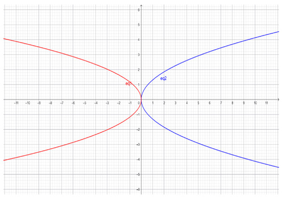
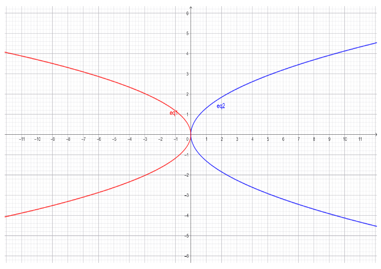
• By substituting the RHS of (47) into (57), we obtain:

  $$\begin{array}{c}\hfill \begin{array}{ccc}\hfill {\displaystyle \frac{dx}{dt}}& =\hfill & 0.93788·(z_1+z_2^2)+0.34694·\left(2z_1\right)\\ \hfill {\displaystyle \frac{dy}{dt}}& =\hfill & -0.34694·(z_1+z_2^2)+0.93788·\left(2z_1\right)\end{array}\end{array}$$

  (58)
  According to Remark 1, the slow manifold in ${\mathbb{R}}^2$ is obtained as a curve

  $$0.93788·(z_1+z_2^2)+0.34694·z_1=0,$$

  (59)

  and the fast manifold is given by

  $$-0.34694·(z_1+z_2^2)+0.93788·z_1=0.$$

  (60)
  In Figure 1, we present the fast and slow manifolds given above in the initial coordinates.
  

  Figure 1. Fast manifold (red) and slow manifold (blue) in $z_1$, $z_2$ coordinates.
• After inverting the transformation matrix (56), we have

  $$\left[\begin{array}{c}{z}_1\\ z_2\end{array}\right]=\left[\begin{array}{cc}0.93788& -0.34694\\ 0.34694& 0.93788\end{array}\right]·\left[\begin{array}{c}x\\ y\end{array}\right].$$

  (61)
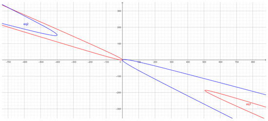
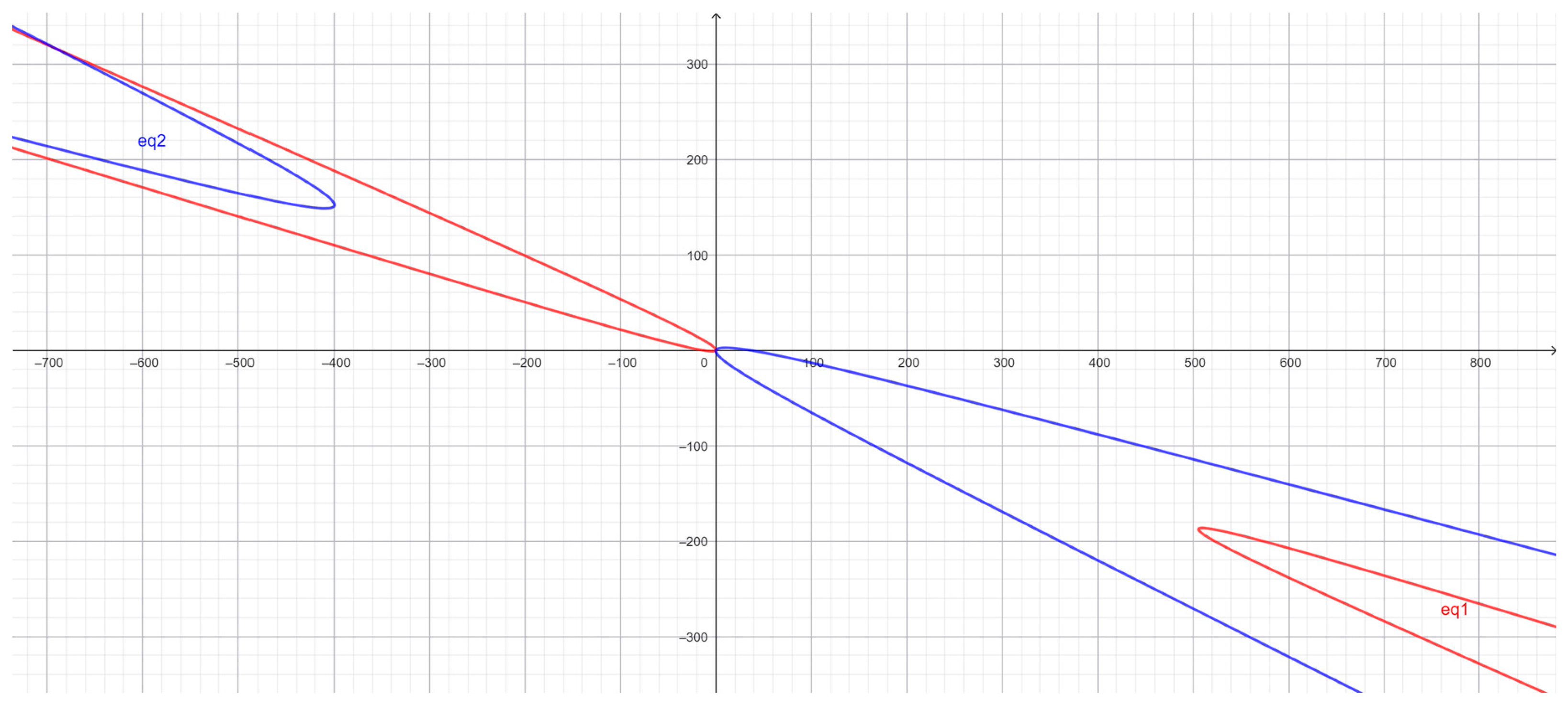
• Finally, from (58) and (61), we obtain (47) in new coordinates when decomposing into fast and slow differential equations (subsystems):

  $$\begin{array}{c}\hfill \begin{array}{ccc}\hfill {\displaystyle \frac{dx}{dt}}& =\hfill & 1.53x-0.57y+0.61xy+0.11x^2+0.82y^2\\ \hfill {\displaystyle \frac{dy}{dt}}& =\hfill & 1.43x-0.53y-0.23xy-0.04x^2-0.3y^2\end{array}\end{array}$$

  (62)
  Again, according to the notation explained in Remark 1, we have the fast manifold in the coordinates $(x,y)$ when the slow subfield equals zero:

  $$1.53x-0.57y+0.61xy+0.11x^2+0.82y^2=0,$$

  (63)

  and a slow manifold is given when the fast subfield equals zero:

  $$1.43x-0.53y-0.23xy-0.04x^2-0.3y^2=0.$$

  (64)
  In Figure 2, we present the fast and slow manifolds given above. Since neither [2] nor [10] provide explicit solution formulas, we also do not provide them here.
  

  Figure 2. Fast manifold (red) and slow manifold (blue) in x, y coordinates.

4. A 3D Computer Modeling Example

Epidemiologists and public health officials use different models for infectious diseases [13]. When an infectious disease threatens a population, we have a simple model that connects the number of susceptible individuals S, infected individuals I and recovered individuals R. In the next example, following the definitions in [14], we construct a suitable three-dimensional SIRD epidemic model, assuming the total population is not invariant.

Example 2.

Create fast and slow subsystems and the corresponding fast and slow manifolds for an SIRD model given with equations:

$$\begin{array}{c}\hfill \begin{array}{cc}\hfill {\displaystyle \frac{dS}{dt}}& =\mu N-\beta {\displaystyle \frac{SI}{N}}-\mu S,\hfill \\ \hfill {\displaystyle \frac{dI}{dt}}& =\beta {\displaystyle \frac{SI}{N}}-(\gamma +\delta +\mu )I,\hfill \\ \hfill {\displaystyle \frac{dR}{dt}}& =\gamma I-\mu R,\hfill \end{array}\end{array}$$

(65)

where the additional variable relation

$$N\left(t\right)=S\left(t\right)+I\left(t\right)+R\left(t\right)$$

enables the system to be genuinely three-dimensional, since there is no conservation law for $S\left(t\right)+I\left(t\right)+R\left(t\right)$. The model is suitable for decomposition according to the algorithm presented in Section 3 and justified by Theorem 1.

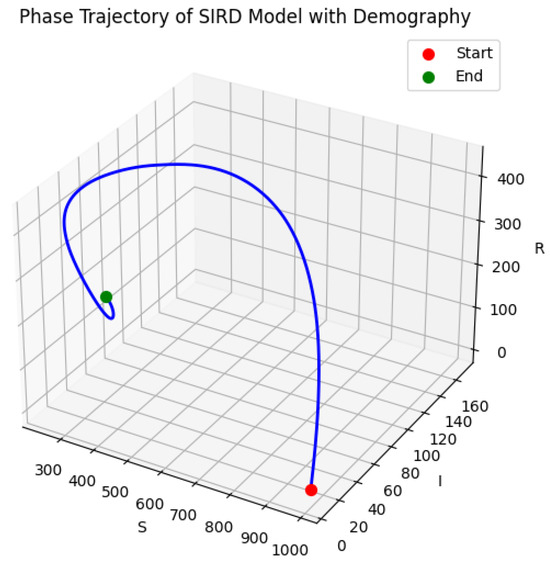
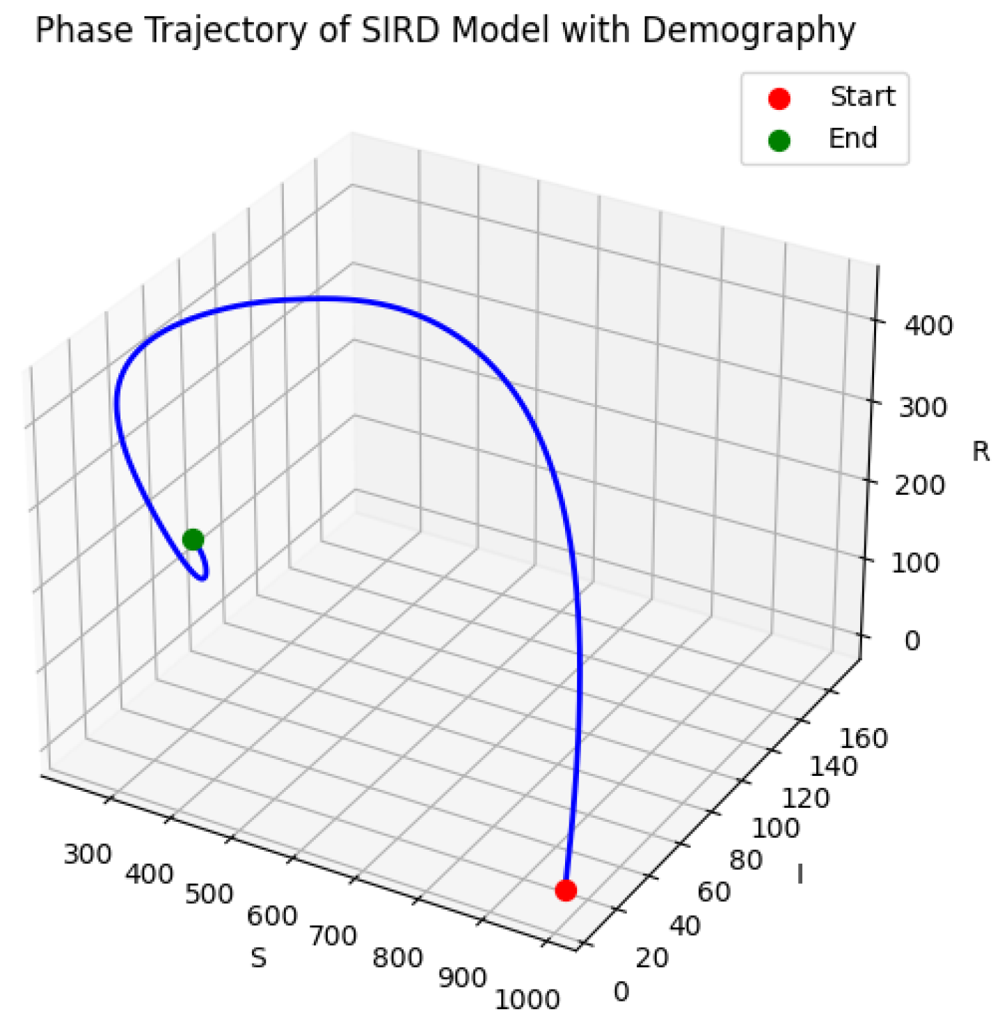
The parameters in (65) are the natural birth and death rate $\mu$, transmission rate $\beta$, recovery rate $\gamma$, and disease-induced mortality rate $\delta$. Different from above, in Figure 3, we show a representative phase trajectory of the SIRD system in the three-dimensional state space $(S,I,R)$, illustrating the true 3D dynamics induced by vital processes.

Figure 3. Phase trajectory of the $SIRD$ system in $(S,I,R)$ space.

Following the methods section (Section 2), an ODE transformation depends on the proper base choice from the points in (16), so we randomly simulate several choices until we find the maximum gap by (20). Unlike manual calculation in the previous section’s example, now we carry out the steps using the computer program Python 3.10.12 [15]. In the following, we present the algorithm given in Section 3, following step-by-step the previous two-dimensional example. After a randomly generated set

$$\Gamma =\{z_1,z_2,\dots ,z_n\},z_i={[S_i,I_i,R_i]}^T\in {⟨0,8000⟩}^3,$$

(66)

for $|\Gamma |=n=10,000$, we calculate the mean vector field from all vector fields obtained by inserting the points from (66) into the formula:

$$\Phi \left(z_i\right)={(\mu N-\beta \frac{SI}{N}-\mu S,\beta \frac{SI}{N}-(\gamma +\delta +\mu )I,\gamma I_i-\mu R)}^T,$$

(67)

and using the parameters $\beta =0.3,\gamma =0.1,\delta =0.05$, and $\mu =0.01$. By the Python program code, we follow the steps in the procedure given in Section 2 to shrink the phase space with randomly generated points $z_i\in \Gamma$ from (66). According to (67), we program the average fields’ calculation:

$$\overline{\Phi }\left(z\right)={\displaystyle \frac{1}{n}}\sum _{i=1}^n\Phi \left(z_i\right),$$

(68)

and obtain ${\Gamma }_{cs}=\{z_i,|\Phi \left(z_i\right)|\ge |\overline{\Phi }\left(z\right)\left|\right\}$, analogue to step [5] from Section 3. For all points $z_i={[S_i,I_i,R_i]}^T\in {\Gamma }_{cs}$, the program code calculates the average absolute determinant value from $\left(\begin{array}{c}|{\Gamma }_{cs}|\\ 3\end{array}\right)$ triples:

$$\Delta ={\displaystyle \frac{1}{\left(\begin{array}{c}|{\Gamma }_{cs}|\\ 3\end{array}\right)}}\sum _{1\le i<j<k\le \left(\begin{array}{c}|{\Gamma }_{cs}|\\ 3\end{array}\right)}\left|\det \left[\begin{array}{ccc}{S}_i& S_j& S_k\\ I_i& I_j& I_k\\ R_i& R_j& R_k\end{array}\right]\right|.$$

(69)

For matrices $B=\left[\begin{array}{ccc}{S}_i& S_j& S_k\\ I_i& I_j& I_k\\ R_i& R_j& R_k\end{array}\right]$ with $det\left[\begin{array}{ccc}{S}_i& S_j& S_k\\ I_i& I_j& I_k\\ R_i& R_j& R_k\end{array}\right]>\Delta$, the program creates symmetric matrices from (17):

$$T{T}^T=\left[{\Phi }_p\left(z_q\right)\right]·{\left[{\Phi }_p\left(z_q\right)\right]}^T,p=1,2,3,q\in \{i,j,k|1\le i<j<k\}.$$

(70)

Indexes $i,j,k$ denote the corresponding columns from matrices selected according to their determinants being greater than the average. At the same time, the program calculates the eigenvalues’ maximum gap for the matrices from (70) according to (20). This results in eigenvalues of the matrix with the maximum gap between ${\lambda }_2$ and ${\lambda }_1$:

$${\lambda }_3=4.24\times {10}^2>{\lambda }_2=1.84\times {10}^2\gg {\lambda }_1=1.66\times {10}^{-4}.$$

(71)

The fast unit eigenvectors ${\mathbf{x}}_3,{\mathbf{x}}_2$ and the slow unit eigenvector ${\mathbf{y}}_1$ corresponding to the eigenvalues from (71) read as follows:

$${\mathbf{x}}_3=\left[\begin{array}{c}0.734\\ 0.145\\ 0.664\end{array}\right],{\mathbf{x}}_2=\left[\begin{array}{c}0.474\\ 0.591\\ -0.653\end{array}\right],{\mathbf{y}}_1=\left[\begin{array}{c}0.487\\ -0.794\\ -0.365\end{array}\right].$$

(72)

The coordinate transformation in $\Omega ={⟨0,8000⟩}^3$ is omitted here, but it decomposes (65) first, as in step [15] in Section 3:

$$\begin{array}{cc}\hfill {\displaystyle \frac{d{x}_3}{dt}}& =0.734{\displaystyle \frac{dS}{dt}}+0.145{\displaystyle \frac{dI}{dt}}+0.664{\displaystyle \frac{dR}{dt}},\hfill \end{array}$$

(73)

$$\begin{array}{cc}\hfill {\displaystyle \frac{d{x}_2}{dt}}& =0.474{\displaystyle \frac{dS}{dt}}+0.591{\displaystyle \frac{dI}{dt}}-0.653{\displaystyle \frac{dR}{dt}},\hfill \end{array}$$

(74)

$$\begin{array}{cc}\hfill {\displaystyle \frac{d{y}_1}{dt}}& =0.487{\displaystyle \frac{dS}{dt}}-0.794{\displaystyle \frac{dI}{dt}}-0.365{\displaystyle \frac{dR}{dt}}.\hfill \end{array}$$

(75)

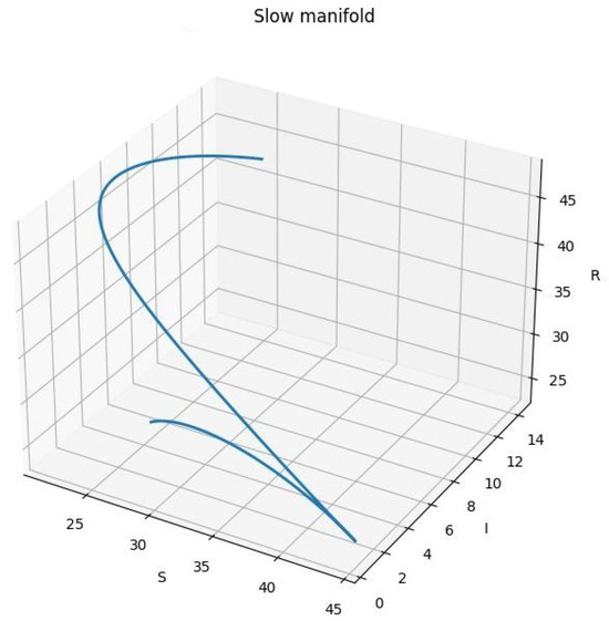
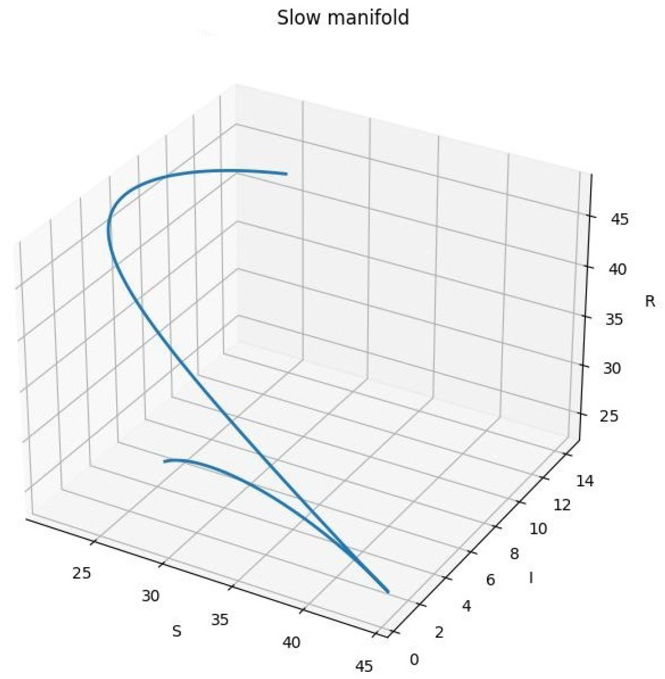
Fast components (73) and (74) vanish on the slow manifold, so we set their RHS to zero. After substituting (65), we obtain the slow manifold as a two-surface intersection given below:

$$\begin{array}{ccc}\hfill 0.734(\mu N-\beta {\displaystyle \frac{S·I}{N}}-\mu S)+0.145(\beta {\displaystyle \frac{S·I}{N}}-(\gamma +\delta +\mu )I)+0.664(\gamma I-\mu R)& =\hfill & \hfill 0,\end{array}$$

(76)

$$\begin{array}{ccc}\hfill 0.474(\mu N-\beta {\displaystyle \frac{SI}{N}}-\mu S)+0.591(\beta {\displaystyle \frac{SI}{N}}-(\gamma +\delta +\mu )I)-0.365(\gamma I-\mu R)& =\hfill & \hfill 0.\end{array}$$

(77)

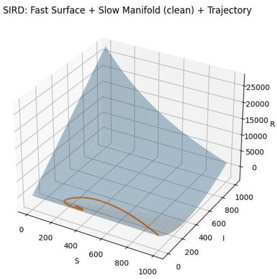
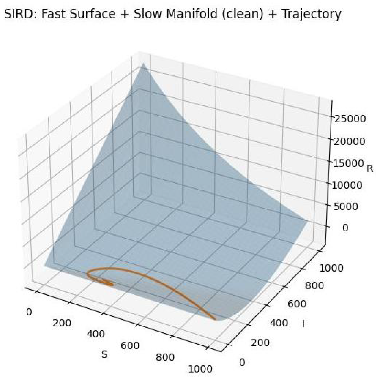
In Figure 4, we draw the slow manifold after substituting coefficients $\beta ,\gamma ,\delta ,\mu$ and taking $N=S+I+R$. In Figure 5, we draw the fast manifold obtained by the disappearance of the slow component, which yields the following equation in the standard coordinates $(S,I,R)$ in $\Omega$:

$$\begin{array}{c}\hfill 0.487(\mu N-\beta {\displaystyle \frac{SI}{N}}-\mu S)-0.794(\beta {\displaystyle \frac{SI}{N}}-(\gamma +\delta +\mu )I)+0.7361(\gamma I-\mu R)=0.\end{array}$$

(78)

We generated figures using numerical simulations implemented in Python, utilizing libraries such as NumPy, SciPy, and Matplotlib. Fast variables $x_3,x_2$ are interpreted as rapid epidemic transients. The slow variable $y_1$ captures the demographic and endemic balance. Thus, the slow manifold, as the manifold when fast variables tend to zero, represents a manifold with a demographic and endemic balance in (65), and it is not an artifact of $S+I+R$ conservation. We do not present the (65) system in coordinates $(x_3,x_2,y_1)$, since we have no reasonable interpretation for now. It is left for further investigation.

Figure 4. Slow manifold in SIRD model as the intersection of the surfaces given by (76) and (77).

Figure 5. Fast manifold in SIRD model as a two-dimensional surface given by (78).

5. Marchuk’s Problem Computer Simulation

In this subsection, we decompose Marchuk’s four-variable problem [16], given by a system of Delay Differential Equations (DDEs) in which the second equation contains a time delay [17], representing the body’s response time, since plasma concentration changes after a delay $\tau$. Results on non-oscillation and related criteria for systems of delay equations are given in [18]. Stabilization methods for systems with distributed input delays and feedback-based approaches are relevant in [19]. Asymptotic properties of solutions for Marchuk’s basic disease model have been studied in [20].

By a change of coordinates, we obtain a system analogous to the SPS in Definition 1 but without an explicit $ϵ$ separating fast and slow components. The infectious disease model is written in [21,22] as follows:

$$\begin{array}{cc}\hfill \frac{dV}{dt}& =\beta V\left(t\right)-\gamma F\left(t\right)V\left(t\right)\hfill \\ \hfill \frac{dC}{dt}& =\zeta \left(m\right)\alpha \left(F\right(t-\tau \left)\right)V(t-\tau )-{\mu }_c(C\left(t\right)-C^{*})\hfill \\ \hfill \frac{dF}{dt}& =\rho C\left(t\right)-\eta \gamma F\left(t\right)V\left(t\right)-{\mu }_{f}F\left(t\right)\hfill \\ \hfill \frac{dm}{dt}& =\sigma V\left(t\right)-{\mu }_{m}m\left(t\right).\hfill \end{array}$$

(79)

The initial state $V\left(0\right)=v_0,C\left(0\right)=C^{*},F\left(0\right)=F^{*},m\left(0\right)=0,$ together with constant histories $V\left(t\right)=v_0>0,C\left(t\right)=C^{*}\ge 0,F\left(t\right)=F^{*}\ge 0,m\left(t\right)=0\mathrm{for}t\in [-\tau ,0]$, where $\tau$ is the body response time, is irrelevant to the decomposition provided by the algorithm given in Section 4 and justified in Theorem 1. In the model (79), $V\left(t\right)$ is the antigen concentration rate, $C\left(t\right)$ is the plasma cell concentration rate, $F\left(t\right)$ is the antibody concentration rate, $C^{*}$ and $F^{*}$ are the plasma rate concentration and the antibody concentration of the healthy body, respectively, and $m\left(t\right)$ is the relative features of the body.

It is assumed that over a certain period of time $t\gg \tau$, plasma is renewed as a result of the interaction of antigen and antibody cells. The body’s defense is described by the following function:

$$\zeta \left(m\right)=\left\{\begin{array}{ll}1& ,0\le m<m^{*}\\ \frac{1-m}{1-m^{*}}& ,m^{*}\le m\le 1,\end{array}\right.$$

taking into account the destruction of the normal functioning immune system. According to [23], we move to the dimensionless case by:

$$V\left(t\right)=v\left(t\right)V_m,C\left(t\right)=s\left(t\right)C^{*},F\left(t\right)=f\left(t\right)F^{*}.$$

(80)

Substituting ${\alpha }_1=\beta , {\alpha }_2=\gamma F^{*}, {\alpha }_3=\alpha V_m{\displaystyle \frac{F^{*}}{C^{*}}}, {\alpha }_4={\mu }_f={\displaystyle \frac{\rho C^{*}}{F^{*}}}, {\alpha }_5={\mu }_c,$ ${\alpha }_6=\sigma V_m, {\alpha }_7={\mu }_m, {\alpha }_8=\eta \gamma V_m$ in (80), as is substituted in [24], we obtain the following non-linear dimensionless ODE system:

$$\begin{array}{cc}\hfill \frac{dv}{dt}& ={\alpha }_{1}v\left(t\right)-{\alpha }_{2}f\left(t\right)v\left(t\right)\hfill \\ \hfill \frac{ds}{dt}& ={\alpha }_3\zeta \left(m\right)f(t-\tau )v(t-\tau )-{\alpha }_5\left(s\right(t)-1)\hfill \\ \hfill \frac{df}{dt}& ={\alpha }_4\left(s\right(t)-f(t\left)\right)-{\alpha }_{8}f\left(t\right)v\left(t\right)\hfill \\ \hfill \frac{dm}{dt}& ={\alpha }_{6}v\left(t\right)-{\alpha }_{7}m\left(t\right).\hfill \end{array}$$

(81)

The coefficients in (81), when the state of the organism is critical, are overwritten from [21]: ${\alpha }_1=2.0, {\alpha }_2=0.8, {\alpha }_3=\mathrm{10,000}, {\alpha }_4=0.17, {\alpha }_5=0.5, {\alpha }_6=10, {\alpha }_7=0.12, {\alpha }_8=8$, and $m^{*}=0.3$. By the aforementioned algorithm in Section 4, and for $\tau =1$, we obtain the matrix with the maximum eigenvalue gap between ${\lambda }_3$ and ${\lambda }_4$. The eigenvalues are obtained by the Python program code, available upon request.

$${\lambda }_1=1.01294·{10}^{-4}<{\lambda }_2=5.2098·{10}^{-1}<{\lambda }_3=1.1013·{10}^{+1}\ll {\lambda }_4=2.27595·{10}^8.$$

After calculating the corresponding eigenvectors, we have a new basis ${\displaystyle \{\frac{d{y}_1}{dt},\frac{d{y}_2}{dt},\frac{d{y}_3}{dt},\frac{d{x}_4}{dt}\}}$ in the tangent bundle. In old coordinates, it reads as follows:

$$\begin{array}{ccc}\hfill {\displaystyle \frac{d{y}_1}{dt}}& =& 0.977{\displaystyle \frac{dv}{dt}}+0.152{\displaystyle \frac{ds}{dt}}+0.147{\displaystyle \frac{df}{dt}}-0.000068{\displaystyle \frac{dm}{dt}}\hfill \\ \hfill {\displaystyle \frac{d{y}_2}{dt}}& =& -0.0000036{\displaystyle \frac{dv}{dt}}+0.000214{\displaystyle \frac{ds}{dt}}-0.00066{\displaystyle \frac{df}{dt}}-0.1{\displaystyle \frac{dm}{dt}}\hfill \\ \hfill {\displaystyle \frac{d{y}_3}{dt}}& =& -0.0956{\displaystyle \frac{dv}{dt}}+0.937{\displaystyle \frac{ds}{dt}}-0.336{\displaystyle \frac{df}{dt}}+0.00042{\displaystyle \frac{dm}{dt}}\hfill \\ \hfill {\displaystyle \frac{d{x}_4}{dt}}& =& -0.189{\displaystyle \frac{dv}{dt}}+0.314{\displaystyle \frac{ds}{dt}}+0.93{\displaystyle \frac{df}{dt}}-0.00055{\displaystyle \frac{dm}{dt}}\hfill \end{array}$$

(82)

In [25], the author interpreted that decomposition into fast $x_4$ and slow $y_1-y_3$ subspaces reveals that rapid antigen–antibody interactions dominate the early phase of infection, whereas plasma cell proliferation, antibody accumulation, and tissue repair govern the long-term trajectory. Marchuk’s model (79) with the given coefficients and considering ${\displaystyle \zeta \left(m\left(t\right)\right)=\frac{1-m\left(t\right)}{0.7}}$ in (81) at time $t\gg \tau$ is read as:

$$\begin{array}{cc}\hfill {\displaystyle \frac{dv}{dt}}& =2.0v\left(t\right)-0.8f\left(t\right)v\left(t\right)\hfill \\ \hfill {\displaystyle \frac{ds}{dt}}& =\mathrm{10,000}{\displaystyle \frac{1-m\left(t\right)}{0.7}}f(t)v(t)-0.5(s(t)-1)\hfill \\ \hfill {\displaystyle \frac{df}{dt}}& =0.17s\left(t\right)-8f\left(t\right)v\left(t\right)\hfill \\ \hfill {\displaystyle \frac{dm}{dt}}& =10v\left(t\right)-0.12m\left(t\right).\hfill \end{array}$$

(83)

By substituting (83) into (82), we obtain the system with a vector field given in $(v,s,f,m)$ phase space. Leaving out note t in a dependent manner, we have

$$\begin{array}{cc}\hfill {\displaystyle \frac{d{y}_1}{dt}}& =1.953v+2169fv-2171mfv-0.051s+0.000008m+0.051\hfill \\ \hfill {\displaystyle \frac{d{y}_2}{dt}}& =-v+3.062fv-3.057mfv-0.000219s+0.012m+0.000107\hfill \\ \hfill {\displaystyle \frac{d{y}_3}{dt}}& =-0.1492v+\mathrm{13,388}fv-\mathrm{13,386}mfv-0.526s-0.00005m-0.469\hfill \\ \hfill {\displaystyle \frac{d{x}_4}{dt}}& =-0.3835v+4478fv-4486mfv+0.0011s+0.157.\hfill \end{array}$$

(84)

Since ${\lambda }_1<{\lambda }_2<{\lambda }_3\ll {\lambda }_4$, we claim that ${\displaystyle \frac{d{y}_1}{dt},\frac{d{y}_2}{dt},}$ and ${\displaystyle \frac{d{y}_3}{dt}}$ span the slow subspace and ${\displaystyle \frac{d{x}_4}{dt}}$ spans the fast subspace in the vector bundle of $\Omega$. Therefore, we have a one-dimensional fast manifold given with the equation system

$$\begin{array}{cc}\hfill 1.953v+2169fv-2171mfv-0.051s+0.000008m+0.051& =0\hfill \\ \hfill -v+3.062fv-3.057mfv-0.000219s+0.012m+0.000107& =0\hfill \\ \hfill -0.1492v+\mathrm{13,388}fv-\mathrm{13,386}mfv-0.526s-0.00005m-0.469& =0.\hfill \end{array}$$

(85)

On the other hand, the three-dimensional slow submanifold is given with the equation

$$-0.3835v+4478fv-4486mfv+0.0011s+0.157=0.$$

(86)

If we change the coordinates in (84),

$$\begin{array}{ccc}\hfill v& =& 0.97766y_1-0.00002y_2-0.09527y_3-0.18895x_4\hfill \\ \hfill s& =& 0.15252y_1+0.00210y_2+0.93711y_3+0.31446x_4\hfill \\ \hfill f& =& 0.14718y_1-0.00662y_2-0.33576y_3+0.93069x_4\hfill \\ \hfill m& =& -0.00068y_1-9.99995y_2+0.00422y_3-0.00546x_4.\hfill \end{array}$$

(87)

we obtain system (81) in coordinates $\{y_1,y_2,y_3,x_4\}$ by transformation (82). Because we cannot draw it and we do not have a reasonable interpretation of this notation, we have not written it. Moreover, the system appears to be enormous.

Biologically, the fast variable corresponds to the immediate immune response to balancing the viral load, and the slow variables correspond to long-term immunity or demographic changes. For more details, see [25].

We emphasize that we do not linearize the Marchuk DDE system, nor do we claim to compute its characteristic quasi-polynomial roots. A full spectral analysis of the DDE explained in [26] is a separate problem outside the present decomposition objective. Methods for stability estimates of uncertain neutral delay systems, relevant to robustness analysis of Marchuk-type DDEs, are given in [27]. Instead, for the chosen response time $\tau =1$, we apply the coordinate-decomposition algorithm described in previous Sections and supported by Theorem 1.

6. Conclusions

This paper is inspired by an algorithm from [2] that transforms an $ODE$ system a system separated into fast and slow subsystems by changing the coordinates in the problem domain. Since in [2,10,11,28] we have not found any proposed theorem, we have justified an algorithm similar to those in [2] by proving Theorem 1. With examples for two and three dimensions, we explain the steps of the algorithm and give some interpretation. Furthermore, we continue to explore Marchuk’s proposed infectious disease model with a new approach based on the algorithm proposed in the paper. Describing the infectious disease process is more complex, and dividing the Marchuk’s model into slow and fast processes is a challenge of interest for engineering applications in system decompositions’ engineering applications. In particular, it is a challenge for further computational simulations.

References

- Chirkov, M.V.; Rusakov, S.V. Modeling Discrete Control of Antiviral Immune Response under Uncertainty. Math. Mech. Inform. 2021, 53, 52–56. [Google Scholar] [CrossRef] [Scilit]
- Nave, O. Singularly Perturbed Vector Field Method (SPVF) Applied to Combustion of Monodisperse Fuel Spray. Differ. Equ. Dyn. Syst. 2019, 27, 57–74. [Google Scholar] [CrossRef] [Scilit]
- Nave, O. Modification of Semi-Analytical Method Applied System of ODE. Mod. Appl. Sci. 2020, 14, 75–81. [Google Scholar] [CrossRef] [Scilit]
- Rusakov, S.V.; Chirkov, M.V. Identification of Parameters and Control in Mathematical Models of Immune Response. Russ. J. Biomech. 2014, 18, 259–269. [Google Scholar]
- Nave, O. A mathematical model for treatment using chemo-immunotherapy. Heliyon 2022, 8, e09288. [Google Scholar] [CrossRef] [Scilit] [PubMed]
- Picard, É. Traité d’Analyse. Tome II: Fonctions Harmoniques et Fonctions Analytiques; Introduction à la Théorie des Équations Différentielles, Intégrales Abéliennes et Surfaces de Riemann; Gauthier-Villars: Paris, France, 1893. [Google Scholar]
- Lindelöf, E.L. Sur l’application de la méthode des approximations successives aux équations différentielles ordinaires du premier ordre. Compt. Rend. Hebd. Seances Acad. Sci. 1894, 116, 454–457. Available online: http://gallica.bnf.fr/ark:/12148/bpt6k3074r (accessed on 20 November 2025).
- Teschl, G. Ordinary Differential Equations and Dynamical Systems. In Graduate Studies in Mathematics; American Mathematical Society: Providence, RI, USA, 2012; Volume 140. [Google Scholar]
- Walter, W. Ordinary Differential Equations. In Graduate Texts in Mathematics; Springer: New York, NY, USA, 1998. [Google Scholar]
- Bykov, V.; Goldfarb, I.; Gol’dshtein, V. Singularly perturbed vector fields. J. Phys. Conf. Ser. 2006, 55, 28–44. [Google Scholar] [CrossRef] [Scilit]
- Bykov, V.; Goldshtein, V.; Maas, U. Scaling Invariant Interpolation for Singularly Perturbed Vector Fields (SPVF). In Coping with Complexity: Model Reduction and Data Analysis; Gorban, A., Roose, D., Eds.; Lecture Notes in Computational Science and Engineering; Springer: Berlin/Heidelberg, Germany, 2011; Volume 75. [Google Scholar] [CrossRef] [Scilit]
- Bershadsky, M. GeoGebra Classic. Available online: https://www.geogebra.org/classic (accessed on 1 January 2026).
- Chambers, R.B. The Role of Mathematical Modeling in Medical Research: “Research Without Patients?”. MSPH Ochsner J. 2000, 2, 218–223. [Google Scholar]
- Melikechi, O.; Young, A.L.; Tang, T.; Bowman, T.; Dunson, D.; Johndrow, J. Limits of epidemic prediction using SIR models. J. Math. Biol. 2022, 85, 36. [Google Scholar] [CrossRef] [Scilit] [PubMed]
- Python Software Foundation. Download Python 3.10.12. Available online: https://www.python.org/downloads/release/python-31012/ (accessed on 31 December 2025).
- Bodnar, M.; Forys, U. Behaviour of Solutions to Marchuks model depending on a time delay. Int. J. Appl. Math. Comput. Sci. 2000, 10, 97–112. Available online: https://zbc.uz.zgora.pl/dlibra/publication/65053/edition/58435/behaviour-of-solutions-to-marchuk-s-model-depending-on-a-time-delay-bodnar-marek-forys-urszula?language=en&utm_source=openai (accessed on 12 December 2025).
- Goebel, G.; Munz, U.; Allgower, F. Stabilization of linear systems with distributed input delay. In Proceedings of the 2010 American Control Conference, Baltimore, MD, USA, 30 June–2 July 2010; IEEE: New York, NY, USA.
- Berezansky, L.; Braverman, E.; Domoshnitsky, A. On nonoscillation of systems of delay equations. Funkc. Ekvacioj 2011, 54, 275–296. [Google Scholar] [CrossRef] [Scilit]
- Mazenc, F.; Niculescu, S.I.; Bekaik, M. Stabilization of time-varying nonlinear systems with distributed input delay by feedback of plant’s state. IEEE Trans. Autom. Control 2013, 58, 264–269. [Google Scholar] [CrossRef] [Scilit]
- Skvortsova, M. Asymptotic Properties of Solutions in Marchuk’s Basic Model of Disease. Funct. Differ. Equ. 2017, 24, 127–135. [Google Scholar]
- Marchuk, G.I. Mathematical Modelling of Immune Response in Infection Diseases. In Mathematics and Its Applications; Springer: Berlin/Heidelberg, Germany, 1997. [Google Scholar]
- Bershadsky, M.; Shaikhet, L. Stability Analysis of a Mathematical Model for Infection Diseases with Stochastic Perturbations. Mathematics 2025, 13, 2265. [Google Scholar] [CrossRef] [Scilit]
- Domoshnitsky, A.; Volinsky, I.; Bershadsky, M. Around the Model of Infection Disease: The Cauchy Matrix and Its Properties. Symmetry 2019, 11, 1016. [Google Scholar] [CrossRef] [Scilit]
- Bershadsky, M.; Chirkov, M.; Domoshnitsky, A.; Rusakov, S.; Volinsky, I. Distributed Control and the Lyapunov Characteristic Exponents in the Model of Infectious Diseases. Complexity 2019, 2019, 5234854. [Google Scholar] [CrossRef] [Scilit]
- Naftaliyev, S. Mathematical and Software Modeling of Infection Spread Under Stochastic Perturbations: Analysis of the Marchuk Model Using the SPVF Method. Master’s Thesis, Shamoon College of Engineering, Department of Software Engineering, Beer Sheva, Israel, 2025. [Google Scholar] [CrossRef]
- Kolmanovskii, V.B.; Nosov, V.R. Stability of Functional Differential Equations; Academic Press Inc.: Cambridge, MA, USA, 1986; pp. 90–94. [Google Scholar]
- Domoshnitsky, A.; Gitman, M.; Shklyar, R. Stability and estimate of solution to uncertain neutral delay systems. Bound. Value Probl. 2014, 2014, 55. [Google Scholar] [CrossRef] [Scilit]
- Bykov, V.; Goldfarb, I.; Gol’dshtein, V. Novel numerical decomposition approaches for multiscale combustion and kinetic models. J. Phys. Conf. Ser. 2005, 22, 1–29. [Google Scholar] [CrossRef] [Scilit]
Disclaimer/Publisher’s Note: The statements, opinions and data contained in all publications are solely those of the individual author(s) and contributor(s) and not of MDPI and/or the editor(s). MDPI and/or the editor(s) disclaim responsibility for any injury to people or property resulting from any ideas, methods, instructions or products referred to in the content. |
© 2026 by the authors. Licensee MDPI, Basel, Switzerland. This article is an open access article distributed under the terms and conditions of the Creative Commons Attribution (CC BY) license.