Article

Limits of Classical Immune Response Models

1
Department of Computer Science, Shamoon College of Engineering, Beer Sheva 8410802, Israel
2
Department of Software Engineering, Shamoon College of Engineering, Beer Sheva 8410802, Israel
*
Author to whom correspondence should be addressed.
Computation 2026, 14(5), 108; https://doi.org/10.3390/computation14050108
Submission received: 22 March 2026 / Revised: 18 April 2026 / Accepted: 20 April 2026 / Published: 8 May 2026
(This article belongs to the Section Computational Biology)

Abstract

We analyze parameter identifiability in a Marchuk-type immune-response model using longitudinal whole-blood transcriptomic signatures from the influenza challenge. Latent states are extracted from curated gene signatures derived from nine symptomatic and eight asymptomatic subjects. The governing delay differential equations are cast in a linear-in-parameters form; derivatives are estimated by smoothing splines, coefficients are fit by ridge regression, and the delay τ is selected by grid search. We find that the parameters governing viral and innate dynamics are consistently identifiable, with low relative error, and are highly determined, whereas adaptive-immunity and tissue-damage parameters are poorly constrained by transcriptomics alone. Introducing a small additive background term and tissue dependence markedly reduces residual variance and stabilizes estimates. Symptomatic patients exhibit a characteristic regulatory delay near 21 h. These results show that aggregated transcriptomic time series can reliably identify some subsystems of classical immune models, but that adaptive immunity and damage dynamics require explicit structural extensions or additional data modalities. The study provides a practical identification pipeline and concrete guidance on model extensions needed for transcriptomic-driven mechanistic inference.

1. Introduction

Mathematical models are valuable for understanding how infectious diseases work and how pathogens and the host immune system interact in complicated ways. The Marchuk framework is the most notable of these models because it is based on biological processes. Using a set of nonlinear ordinary differential equations ( O D E s), it demonstrates how pathogen load, immune cell populations, antibody production, and regulatory mechanisms work together. The values of the model’s coefficients are very important for how accurate its predictions are [1].
It is not easy to find these coefficients. We cannot directly measure many biological processes in life forms, such as how fast pathogens replicate, how fast the immune system activates, how fast antibodies break down, and how fast effector cells respond. To estimate the parameters, we must fit the O D E system to experimental or clinical data, ensuring that the resulting values are biologically significant and mathematically stable. Most of the time, this process includes optimizing the numbers, looking at sensitivity, and carefully checking the identifiability of the model.
This work aims to develop a systematic approach for deriving the coefficients of the Marchuk disease model. We want to generate sets of parameters that accurately show how diseases progress, and let us run reliable simulations of immune-pathogen dynamics by combining theoretical knowledge with computational estimation methods. A clear way to find coefficients not only makes the model more scientifically, valid but also makes it more useful for scenario analysis, treatment assessment, and other areas of immunology and epidemiology.
Each equation in Marchuk’s infectious disease model represents a distinct biological process, including pathogen replication, immune activation, and antibody degradation. Before estimating parameters, the complete O D E system was written symbolically, and all state variables and coefficients were defined based on their biological meanings to ensure mathematical consistency and biological relevance. In this subsection, we transform the O D E system with four variables into the State Parameter Separation ( S P S ) system.

2. Data and Biological State Construction

In this study, we used the publicly available transcriptomic dataset G S E 30550 , obtained from Gene Expression Omnibus (GEO) [2]. The dataset contains longitudinal whole-blood gene expression profiles collected from human volunteers experimentally infected with Influenza A ( H 3 N 2 ). Based on the presence and intensity of influenza-related symptoms, subjects were categorized into symptomatic ( n = 9 ) and asymptomatic ( n = 8 ) groups while being clinically monitored.
Measurements of gene expression were taken at several intervals during the early stages of infection, the peak of immune activation, and the recovery that followed. Although the dataset was not initially intended for direct mathematical system identification, this temporal structure makes it especially useful for studying immune response dynamics.
Furthermore, the dataset offers molecular-level observations instead of precise measurements of tissue damage, immune cell counts, viral load, or cytokine concentrations. Consequently, there is no one-to-one correspondence between the data and the traditional immune model variables. Rather, they record the state of biological processes that are activated during the host’s reaction to an infection.
As summarized in Table 1, G S E 30550 was designed to characterize transcriptional responses to influenza infection rather than to directly observe the state variables used in mathematical immune response models. Consequently, gene expression profiles must be interpreted as indirect, noisy, and temporally delayed proxies of immune system activity.
This characteristic should not be interpreted as a weakness of the dataset. Instead, it enables a critical evaluation of whether classical immune response models remain structurally valid when confronted with real molecular data, rather than idealized or directly observable quantities. Similar challenges and opportunities have been discussed extensively in systems immunology and data-driven modeling studies [3].

2.1. Motivation for Signature-Based State Construction

Mathematical immune response models, including the classical Marchuk immune response model [4,5], describe system dynamics using aggregated state variables that are not directly observable in transcriptomic data. To bridge this gap, we adopt a signature-based abstraction strategy, in which biologically coherent groups of genes are selected to represent specific immune processes.
Each gene signature is constructed based on established biological function and prior evidence from influenza and viral immunology studies. The goal is not to recover exact biological quantities but to define latent dynamical states whose temporal behavior reflects the activation and regulation of key immune mechanisms. These latent states are denoted by V ( t ) , F ( t ) , C ( t ) and M ( t ) corresponding to viral stress, cytokine signaling, adaptive immunity, and tissue damage, respectively.
This approach reduces dimensionality, improves interpretability, and enables mechanistic reasoning from high-dimensional gene expression data. Signature-based representations have been successfully applied in numerous system immunology studies [3,6] and provide a natural bridge between molecular data and low-dimensional dynamical models. In software-engineering terms, each signature is a stable, testable feature extractor that maps noisy omics data to low-dimensional signals for downstream identification and validation. This abstraction allows the resulting dynamical model to be evaluated, refactored, and extended in a manner analogous to that of modular software components.

2.2. Transcriptomic Proxies for Latent State Variables

The four biological gene signatures used in this study are summarized in Table 2. Each signature is designed to capture a distinct immunological process that aligns with a corresponding state variable in the mathematical model; these state variables are formally defined in Section 3. This approach follows the general logic of gene-set and modular transcriptomics: rather than fitting models to thousands of genes, one aggregates curated markers that reflect a biological program (stress response, interferon signaling, cytotoxic lymphocytes, neutrophil/tissue injury), which improves interpretability and engineering reproducibility [3,6]. These signatures operationalize the abstract state variables of the mathematical model by mapping them to biologically grounded transcriptomic programs.
The V state is constructed using genes associated with unfolded protein response (UPR)/ER stress (HSPA5/HSP90B1, XBP1, DDIT3, ATF4/ATF6, ERN1, and downstream processing factors), oxidative/redox regulators (HMOX1, SOD2, TXN/TXNRD1, NQO1, GCLM/GCLC, PRDX1), hypoxia/glycolysis shift markers (SLC2A1, HK2, PFKP, ALDOA, ENO1, LDHA, PDK1, BNIP3), and immediate-early transcriptional responders (JUN, FOS, ATF3, EGR1). Influenza A infection is known to interact with ER-stress/UPR pathways and to reshape host stress programs as part of viral replication and host defense, motivating the inclusion of UPR core genes [7]. Stress-triggered transcriptional regulators (AP-1 axis such as JUN/FOS, and immediate-early genes) frequently appear in host–influenza interaction maps and infection-response programs, supporting their role as a compact “cellular stress” readout [8].
The F signature is centered on type I interferon ( I F N B 1 ) and inflammatory cytokines/chemokines (IL1A/IL1B/IL18, IL6, TNF, IFNG, CXCL8, CXCL10, CCL2/CCL4/CCL5). Type I interferons are canonical early antiviral mediators and shape downstream cytokine cascades; importantly, influenza can trigger both protective and pathology-amplifying interferon-associated programs, which aligns this signature with “innate response intensity” [9].
The C signature uses T cell markers and cytotoxic effector genes: CD3D/CD3E/CD3G (TCR complex), CD4 and CD8A/CD8B lineages, IL7R and TCF7 (T cell maintenance and memory/stem-like features), and cytotoxic granule genes PRF1, GZMB, and NKG7, plus activation markers (CD69, CD2). These genes reflect T cell recruitment/activation and cytotoxic capacity, which are central components of antiviral adaptive immunity in influenza [10].
The M signature emphasizes neutrophil and myeloid activation markers (S100A8, S100A9, S100A12, LCN2, CEACAM8), neutrophil granule/enzymatic effectors (ELANE, MPO, AZU1, CTSG), matrix remodeling mediators (MMP8/MMP9), monocyte/macrophage markers (CD14, LST1, ITGAM, CD68, CSF1R, CD163), and SERPINE1. Severe influenza has been repeatedly associated with strong innate inflammatory infiltration and neutrophil-linked signatures; these programs are also mechanistically connected to lung injury and barrier dysfunction [11]. In addition, MMP9 has been directly implicated in influenza-associated lung pathology in experimental systems, supporting its inclusion as a damage-related marker [12]. In this work, M ( t ) should be interpreted as a normalized latent indicator of inflammatory tissue damage and innate immune-mediated injury, rather than a direct measurement of organ mass or structural loss.
This construction enables a structural, rather than a purely numerical, assessment of classical immune response models when confronted with real-world molecular data.

2.3. Interpretation as Latent Dynamical States

The gene signatures defined above are interpreted as latent dynamical states rather than direct biological measurements. Each state summarizes the activity of a biological process that evolves over time and influences other components of the immune response. Caution is warranted when extrapolating peripheral gene-expression signatures to organ-level dynamics, as cross-system transcriptomic concordance can be limited [13]. Although transcriptomic signals are indirect, delayed, and influenced by heterogeneous cell populations, their temporal structure provides valuable information about system dynamics.
By focusing on relative temporal behavior rather than absolute values, this approach enables a principled comparison between molecular data and the structural assumptions of classical immune response models. Gene signatures function as a biologically interpretable nexus between transcriptomics and mathematical immunology.

3. Mathematical Model Framework

We adopt a classical Marchuk-type immune response model in a dimensionless form, which represents the coupled dynamics of (i) viral/antigen activity, (ii) antibody-mediated response, (iii) antibody-producing cell activity, and (iv) tissue damage under infection [14,15]. The model is written as a nonlinear dynamical system with a single discrete delay that represents the biological latency between antigen recognition and the appearance of an effective humoral response.
In the original notation, the state variables are v ( t ) , s ( t ) , f ( t ) , and m ( t ) , and the coefficients are α 1 , , α 8 [16]:
d v d t = α 1 v ( t ) α 2 f ( t ) v ( t ) ,
d f d t = α 4 s ( t ) f ( t ) α 8 f ( t ) v ( t ) ,
d s d t = α 3 ζ ( m ( t ) ) f ( t τ ) v ( t τ ) α 5 s ( t ) 1 ,
d m d t = α 6 v ( t ) α 7 m ( t ) .
Throughout this paper, we keep the same mathematical structure, but align symbols with our transcriptomic latent states: v ( t ) V ( t ) (viral/host stress proxy), f ( t ) F ( t ) (cytokine/innate activation proxy), s ( t ) C ( t ) (adaptive/humoral proxy; in our implementation we use C for this state), and m ( t ) M ( t ) (damage proxy). This is a notational mapping only; the dynamical couplings remain those in Equations (1)–(4).
Equation (1) describes viral growth at rate α 1 and suppression through interaction with the immune response at rate α 2 f ( t ) v ( t ) . The bilinear term reflects the idea that clearance increases when both antigen and immune activity are high. Equation (3) governs the dynamics of the antibody-producing compartment (or an effective adaptive/humoral activation state). The constant 1 is the physiological baseline, so α 5 ( s ( t ) 1 ) drives relaxation back toward a healthy equilibrium in the absence of stimulation. The production term depends on past antigen and immune activity, f ( t τ ) v ( t τ ) , introducing the delay τ 0 that represents activation, proliferation, and differentiation time in the immune cascade [14,15]. Equation (2) captures antibody/immune-effector dynamics. The term α 4 ( s f ) pulls f ( t ) toward the current adaptive/humoral level s ( t ) , while α 8 f ( t ) v ( t ) represents consumption or neutralization activity coupled to antigen presence. Finally, Equation (4) models damage accumulation proportional to viral activity ( α 6 v ) and recovery/regeneration proportional to existing damage ( α 7 m ), yielding a stable return toward m ( t ) = 0 when the antigen is absent [14,17,18], and reduces organ health modulation ζ ( m ) . A key feature of this family of models is the non-increasing, non-negative function ζ ( m ) , which reduces immune production when tissue damage becomes severe. We use the classical continuous piecewise definition:
ζ ( m ) = 1 , 0 m < m , 1 m 1 m , m m 1 ,
where m ( 0 , 1 ) is the maximal fraction of damaged tissue for which normal immune functioning is still possible. For mild damage ( m < m ), the immune system operates at full effectiveness ( ζ = 1 ). Beyond this threshold, effectiveness decreases linearly and reaches ζ = 0 at m = 1 , representing total loss of functional tissue. In our transcriptomic setting, m ( t ) is interpreted as a normalized latent damage indicator rather than direct organ mass, but Equation (5) preserves the original structural meaning: damage feeds back negatively on immune production [14].
Although the system is nonlinear in states, each equation is linear in its coefficients. For example, the right-hand side (RHS) of Equation (1) is a linear combination of regressors v ( t ) and f ( t ) v ( t ) with coefficients ( α 1 , α 2 ) . The same applies to Equations (1)–(3) once τ (and, when used, ζ ( m ) ) is fixed. This ”linear-in-parameters” form enables parameter estimation from time series by constructing a regressor matrix and solving a (regularized) least-squares problem in derivative space. In practice, τ is unknown and is therefore selected by grid search, because it changes the lagged values v ( t τ ) and f ( t τ ) that best explain the observed derivatives [15,19]. This four-state delayed formulation has been examined in control and stabilization contexts in [4].

4. Parameter Identification and Estimation Methodology

This section describes the end-to-end identification pipeline used to estimate the coefficients α 1 , , α 8 in the dimensionless Marchuk-style system (see Section 3). Rather than searching a large nonlinear model space, as in sparse identification approaches [20], we exploit the Marchuk model’s linear-in-parameters structure to obtain stable ridge estimates.
Our core idea is to transform each differential equation into a linear regression problem in the unknown coefficients by (i) constructing smoothed state trajectories and their derivatives, (ii) building a design matrix from the right-hand-side regressors, (iii) solving a regularized least squares problem, and (iv) validating numerical reliability via error bars and conditioning diagnostics. Figure 1 presents the deterministic parameter identification workflow adopted in this study. The pipeline begins with data preprocessing, where gene-signature trajectories are cleaned and normalized. This is followed by derivative estimation, achieved through local polynomial smoothing and analytical differentiation. The regression design stage constructs linear-in-parameter representations of the governing differential equations. Parameter estimation is then performed using ridge-regularized least squares. The final stages involve diagnostic evaluation, including residual inspection, uncertainty quantification, and conditioning analysis, and conclude with artifact export, which preserves fitted parameters, diagnostics, and visualizations to ensure full reproducibility.

4.1. Methodological Rationale: Derivative Matching Versus Forward Integration

The classical approach to DDE parameter identification consists of numerically integrating the system from specified initial conditions and minimizing the discrepancy between simulated trajectories and observed data [21]. While theoretically rigorous, this approach faces three structural obstacles in the present setting. First, the latent state initial conditions V ( 0 ) , F ( 0 ) , C ( 0 ) , M ( 0 ) are not directly observable—they are constructed from transcriptomic signatures and carry their own measurement uncertainty. Estimating them as additional free parameters alongside α 1 , , α 8 yields a 12-dimensional nonlinear optimization problem for only n = 16 observations per patient, which is severely underdetermined and provides no guarantee of convergence to a meaningful solution.
Second, for fixed τ , the Marchuk equations are linear in the unknown coefficients (see Section 4.5), which admits closed-form ridge-regularized estimates with transparent diagnostics ( R 2 , residual variance, conditioning, relative errors). Classical analytical and semi-analytic treatments of the Marchuk model [22] motivate caution when choosing numerical integration schemes for parameter fitting. Forward integration with Runge–Kutta methods destroys this linearity, requiring nonlinear optimization over a non-convex landscape.
Third, numerical integration of a DDE over a 108-h horizon accumulates truncation and round-off errors that interact with the sparsity of observations. Analytic differentiation of a smoothing spline (Equation (9)) is numerically more stable and avoids this error propagation. The derivative-matching approach is well-established in the systems biology literature [23,24,25] and is particularly appropriate when time series are short, initial conditions are uncertain, and interpretable uncertainty bounds are required.

4.2. Data Alignment, Cleaning, and Fitting Window

Let { t i } i = 1 N denote the (possibly irregular) sampling times for a given phenotype group (symptomatic or asymptomatic). After loading the transcriptomic-derived latent state trajectories V ( t i ) , F ( t i ) , C ( t i ) , and M ( t i ) , we apply a deterministic preprocessing procedure consisting of: (i) casting all variables into numeric form, (ii) removing observations containing NaN or infinite values, (iii) sorting the data chronologically, and (iv) restricting the analysis to a fixed fitting window
t i [ T min , T max ] ,
which in our experiments corresponds to [ 0 , 108 ] hours after infection.
This preprocessing step ensures that all subsequent computations are well-defined, reproducible, and independent of implementation-specific rules.
When delay terms are introduced in the model (Section 4.4), the effective sample size becomes an explicit function of the delay parameter τ . Since delayed regressors such as V ( t τ ) or F ( t τ ) are only defined when the shifted time point lies within the observed data range, only indices satisfying
I τ = { i t i τ [ T min , T max ] }
are retained for parameter estimation. The resulting number of usable observations is therefore
N τ = | I τ | N .
As a consequence, each value of τ defines a distinct regression problem with its own effective sample size and design matrix. This explains why different delay values produce different values of n in the grid-search results, even though the same original dataset is used throughout.
Importantly, this reduction in sample size is not an artifact of the estimation procedure but a structural property of delay differential equation models. Larger delays systematically exclude early time points, reflecting the fact that delayed biological effects cannot be inferred before the corresponding causal signal has been observed. Each ( τ , N τ ) pair therefore represents a valid and self-consistent identification problem, enabling a principled comparison of model performance across different delay hypotheses.

4.3. Smoothing and Numerical Differentiation (Construction of LHS)

The dataset provides latent state trajectories but does not directly provide their time derivatives V ˙ , F ˙ , C ˙ , M ˙ . Naive finite-difference schemes are known to be unstable for irregularly sampled and noisy biological data. Therefore, derivatives are estimated by first constructing smooth approximations of the state trajectories and then differentiating these approximations analytically.
For a generic latent state x ( t ) , where x { V , F , C , M } , we approximate its temporal evolution using a cubic smoothing spline g ( t ) . The spline is obtained by minimizing a regularized least-squares objective x ^ ( t ) of the form
x ^ ( t ) = arg min g S 3 i = 1 n x ( t i ) g ( t i ) 2 + λ g ( t ) 2 d t ,
where S 3 denotes the space of cubic splines and λ > 0 is a smoothing parameter controlling the trade-off between fidelity to the data and smoothness of the fitted trajectory, n = 16 number of observations.
The time derivative is then computed analytically as
x ˙ ( t ) d d t x ^ ( t ) ,
which yields stable derivative estimates without amplifying measurement noise.
The fitted splines and their derivatives are evaluated on a dense and uniform time grid t [ T min , T max ] , producing a consistent left-hand-side (LHS) dataset containing ( t , V , F , C , M , V ˙ , F ˙ , C ˙ , M ˙ ) . The resulting smoothed trajectories and their analytically computed derivatives form a fixed left-hand-side dataset that is reused in all subsequent identification experiments. This separation decouples numerical differentiation from parameter estimation and ensures that model comparison is not confounded by repeated smoothing or differentiation artifacts.

4.4. Delay Handling and Interpolation

Several equations of the classical immune response model include delayed interaction terms, most notably products of the form F ( t τ ) V ( t τ ) . Such delays represent finite biological response times, including signaling cascades, cell activation, and effector recruitment. In the transcriptomic dataset, latent state trajectories are available only at discrete sampling times { t i } i = 1 N . For a given delay τ 0 , the shifted time points t i τ generally do not coincide with the observed sampling grid. Therefore, delayed values must be reconstructed numerically. Practical considerations for handling discrete delays and choosing numerical schemes for parameter identification in Marchuk models are discussed in [26]. A comparison with forward-integration results remains a valuable direction for future work.
For any latent state trajectory x ( t ) and delay τ , we define the lagged signal as
x τ ( t i ) x ( t i τ ) ,
which is approximated by piecewise linear interpolation over the observed data:
x τ ( t i ) interp t i τ ; { ( t j , x ( t j ) ) } j = 1 N ,
where interp ( × ) denotes linear interpolation on the original time grid.
Only those time points for which t i τ lies within the observed interval [ t min , t max ] are retained for model fitting. As a result, the effective sample size depends explicitly on the delay value τ . This explains why different delays lead to different numbers of usable observations in the grid-search results. All delayed regressors appearing in the model equations are constructed using (12). This approach preserves temporal consistency, avoids introducing additional smoothing, and ensures that delay effects are evaluated on the same reconstructed continuous-time representation used for derivative estimation.

4.5. Linear-in-Parameters Regression Form

After constructing smooth estimates of the time derivatives, each differential equation in the model is transformed into a regression problem that is linear in the unknown coefficients. This transformation enables deterministic parameter identification using regularized least-squares techniques and allows for direct interpretation of the estimated coefficients in terms of model structure. Numerical identifiability diagnostics (condition number, relative parameter error) complement structural identifiability analysis as discussed in [27].
For each equation, we write
y = X θ + ε ,
where y R N τ is the vector of estimated derivatives (left-hand side), X R N τ × p is the design matrix constructed from observable regressors (right-hand side), θ R p is the vector of unknown model coefficients, and ε captures model mismatch and residual noise. The effective sample size N τ depends on the delay τ , as discussed in Section 4.4.
Each coefficient α i quantifies the strength of a specific interaction term encoded in the corresponding differential equation. The coefficients do not represent direct biological measurements, but rather effective interaction rates inferred from transcriptomic dynamics.

4.5.1. V-Equation

The viral stress dynamics in Equation (1) are written as
y i = V ˙ ( t i ) , X i = V ( t i ) V ( t i ) F ( t i ) , θ = α 1 α 2 .
Here, α 1 represents the effective self-amplification rate of the viral stress state V ( t ) , capturing the combined effects of viral replication and stress propagation in host cells. The coefficient α 2 quantifies the strength of suppression of viral stress through interaction with the cytokine signaling state F ( t ) . The negative sign is absorbed into the regressor so that α 2 is interpreted as a positive interaction coefficient.

4.5.2. F-Equation

For the cytokine signaling dynamics (2), we define
y i = F ˙ ( t i ) , X i = C ( t i ) F ( t i ) F ( t i ) V ( t i ) , θ = α 4 α 8 .
The coefficient α 4 controls the relaxation rate of the cytokine signaling state F ( t ) toward the adaptive immune state C ( t ) . This term represents an effective regulatory coupling that drives F ( t ) to track the level of adaptive immunity rather than a direct stimulatory interaction. The coefficient α 8 captures the effective attenuation of cytokine signaling through interaction with viral stress, representing consumption, exhaustion, or regulatory feedback mechanisms. As before, the sign convention is embedded in the regressor definition.

4.5.3. M-Equation

The tissue damage dynamics (4) are expressed as
y i = M ˙ ( t i ) , X i = V ( t i ) M ( t i ) , θ = α 6 α 7 .
The coefficient α 6 quantifies the rate at which viral stress contributes to tissue damage accumulation, while α 7 represents the effective recovery or repair rate that drives the damage state M ( t ) back toward baseline. Both coefficients describe net effects aggregated across multiple biological processes.

4.5.4. C-Equation with Delay and Organ-Health Modulation

The adaptive immune response dynamics are described by
C ˙ ( t ) = α 3 ζ M ( t ) F ( t τ ) V ( t τ ) α 5 ( C ( t ) 1 ) ,
where ζ ( M ) modulates immune activation according to tissue health and τ represents a signaling delay.
For parameter identification, the equation is evaluated at discrete time points t i and written in linear-in-parameters form as
y i = C ˙ ( t i ) , X i = ζ M ( t i ) F ( t i τ ) V ( t i τ ) ( C ( t i ) 1 ) , θ = α 3 α 5 .
To ensure numerical stability and balanced regularization, each regressor column is scaled by its maximum absolute magnitude prior to estimation. Ridge regression is then applied in the scaled space, and the resulting coefficients are transformed back to physical units. Parameter uncertainties are obtained from the regularized covariance matrix of the estimator.

4.6. Regularized Estimation: Ridge Regression

Although each differential equation in the proposed framework is linear in parameters, the resulting regression problems are often ill-conditioned. This arises from two main sources. First, regressors can be strongly correlated, for example, V ( t ) and V ( t ) F ( t ) in the viral and antibody equations. Second, numerical differentiation of transcriptomic trajectories amplifies measurement noise, which propagates into the left-hand side of the regression. Together, these effects lead to unstable ordinary least squares estimates and inflated parameter variance.
To address this issue, we employ ridge regression, also known as Tikhonov-regularized least squares. Given the augmented linear model
y = X ˜ θ ˜ + ε ,
the parameter vector is estimated by solving
θ ˜ ^ = arg min θ ˜ X ˜ θ ˜ y 2 2 + λ θ ˜ 2 2 ,
where λ > 0 is the regularization strength.
The solution admits a closed-form expression:
θ ˜ ^ = ( X ˜ X ˜ + λ I ) 1 X ˜ y ,
with I denoting the identity matrix of appropriate dimension.
In this work, λ is chosen as a small fixed constant (typically λ = 10 3 ). This choice does not enforce strong shrinkage but acts as a numerical stabilizer that suppresses the amplification of noise and mitigates multicollinearity. Empirically, we observe that ridge regularization substantially reduces coefficient variance and improves conditioning without altering the qualitative structure of the estimated dynamics.
From an identification perspective, ridge regression introduces a controlled bias–variance trade-off. While the estimates are no longer unbiased in the strict statistical sense, the reduction in variance yields more reliable and interpretable parameters, particularly when derivatives are estimated from noisy transcriptomic data. This trade-off is well aligned with the goal of structural model assessment rather than pointwise prediction.
In the implementation, ridge regression is applied uniformly across all equations (V, F, C, and M), after appropriate scaling of regressors. The same formulation is used for both baseline and γ 0 -augmented models, ensuring consistency when comparing alternative model variants.

4.7. Scaling, Standardization, and SEM-Based Weighting

Prior to parameter estimation, all regression problems are numerically stabilized by scaling the regressors. This step is essential because ridge regularization penalizes coefficients according to their magnitude, and regressors with different numerical ranges would otherwise lead to biased or unstable estimates.
Two scaling strategies are implemented in the identification pipeline, depending on the structure of the regression problem and the availability of uncertainty information.

4.7.1. Max-Absolute Scaling

In the baseline identification setting, each regressor column X × k is scaled by its maximum absolute value;
s k = max i | X i k | ,
and the scaled design matrix is defined as
X i k ( s ) = X i k s k .
Ridge regression is solved in scaled space, and coefficients are mapped back to physical units by
θ ^ k = θ ^ k ( s ) s k .
This normalization improves conditioning while preserving the original mechanistic interpretation of each term.

4.7.2. Weighted Standardization

For regression problems in which regressor magnitudes differ substantially or interaction terms are present, regressors are standardized using weighted mean and variance:
μ k = i w i X i k i w i , σ k 2 = i w i ( X i k μ k ) 2 i w i ,
followed by the transformation;
X i k ( z ) = X i k μ k σ k .
This procedure ensures that ridge regularization acts uniformly across regressors and avoids scale-induced distortions in the estimated interaction coefficients.

4.7.3. SEM-Based Weighting

When standard errors of the mean (SEM) are available from the construction of latent states, they are incorporated through inverse-variance weighting,
w i = 1 SEM i 2 .
In practice, weighted ridge regression is implemented by multiplying each row of the design matrix and the corresponding response value by w i prior to solving the regularized least-squares problem. This approach assigns greater influence to time points with higher confidence and naturally downweights regions with increased transcriptomic uncertainty.
Overall, scaling and weighting are treated as integral components of the identification pipeline. They improve numerical conditioning, stabilize parameter estimates, and enable consistent comparison between different equations and model configurations.

4.8. Grid Search over Delay τ and Model Selection

The delay parameter τ is treated as a discrete hyperparameter and selected via grid search over a finite candidate set of possible delay hours (h):
τ T = { 0 , 5 , 12 , 21 } h .
The candidate set (27) was made to show four different biological stages of the early antiviral response to influenza A infection. The value τ = 0 is a no-delay baseline control. The value τ = 5 h corresponds to the timescale of early type I interferon induction: activation of interferon signaling pathway genes in cells infected with influenza H3N2 has been seen as early as 3–6 h after infection [28,29]. The value τ = 12 h marks the beginning of NK cell activation and the first recruitment of innate effectors. This happens before the peak NK cell infiltration, which happens about 48 h after infection [30]. The value τ = 21 h marks the first signaling window for C D 8 + T-lymphocyte priming in the draining lymph nodes. This starts within the first 24–72 h of pulmonary influenza infection [31].
These four values represent the early innate-to-adaptive transition period and are based on biologically motivated hypotheses rather than data-driven selections. For each τ T , delayed regressors are reconstructed by interpolation as described in Section 4.4. Only time points satisfying t i τ [ t min , t max ] are retained, which leads to a τ -dependent effective sample size N τ .
For each admissible τ , model coefficients are estimated using ridge-regularized least squares with the same scaling and weighting strategy. Model performance is evaluated in derivative space by comparing observed derivatives y i and model predictions y ^ i .
When SEM-based weights are available, delay selection is based on the Weighted Mean Squared Error:
WMSE ( τ ) = i w i ( y i y ^ i ) 2 i w i ,
where w i are inverse-variance weights. If weights are not used, unweighted RMSE or MSE is reported instead.
The optimal delay is defined as
τ = arg min τ T WMSE ( τ ) ,
and is reported together with the corresponding sample size N τ . Explicitly reporting N τ is essential, as increasing delay systematically reduces the amount of usable data and affects statistical reliability.

4.9. Diagnostics: R 2 , Uncertainty, and Conditioning

Model diagnostics are evaluated in derivative space in order to assess the quality of right-hand-side (RHS) identification directly, rather than the accuracy of reconstructed trajectories. This choice avoids artificially inflated goodness-of-fit metrics that may arise from temporal smoothing and numerical integration.

4.10. R 2 in Derivative Space

We adopt diagnostic metrics and pragmatics from systems-identification practice to assess fit and estimator reliability [32]. The goodness of fit is quantified using the coefficient of determination computed on derivative targets:
R 2 = 1 i I τ ( y i y ^ i ) 2 i I τ ( y i y ¯ ) 2 , y ¯ = 1 N τ i I τ y i ,
where y i denotes the estimated derivative (LHS), y ^ i the fitted RHS prediction, and I τ the index set of valid samples for a given delay τ . Evaluating R 2 in derivative space provides a conservative and structurally meaningful assessment of model adequacy.

4.11. Residual Variance

Unexplained variability after fitting is summarized by the residual variance estimate
σ ^ 2 = y y ^ 2 2 N τ p ,
where p is the number of estimated parameters, including the intercept γ 0 when present. This quantity reflects the magnitude of dynamics not captured by the modeled RHS terms.

4.12. Coefficient Uncertainty

The approximate parameter uncertainty is obtained from the ridge-adjusted covariance estimate
Cov ( θ ˜ ^ ) σ ^ 2 ( X ˜ X ˜ + λ I ) 1 ,
from which the standard errors are extracted as the square roots of the diagonal elements. For interpretability, uncertainty is reported using relative error:
RelErr k = SE ( θ ˜ ^ k ) | θ ˜ ^ k | .
Coefficients with relative error exceeding 20 % are considered weakly constrained by the data.

4.13. Conditioning

Numerical identifiability is further assessed using the condition number of the unregularized normal matrix:
κ = cond ( X X ) .
Large values of κ indicate strong collinearity between regressors and increased sensitivity to noise. Conditioning is interpreted jointly with coefficient uncertainty, rather than as an isolated diagnostic.

5. Results

Among the 17 patients listed in Table 1, nine of them have symptoms and eight patients do not have symptoms. Therefore, we divide this section into two sections with results that differ from these conditions. According to the templates given in Section 4.5, we calculate the coefficients { α 1 , , α 8 } . According to the template given in Section 4.2, we calculate the delay time parameter τ . On the basis of n = 16 real measurements from 17 patients each, we loaded N = 200 base data t i [ T min , T max ] = [ 0.0 , 108.0 ] according the spline function g ( t ) used to minimize (9). Assuming it will be more understandable, we divide the section into four parts.
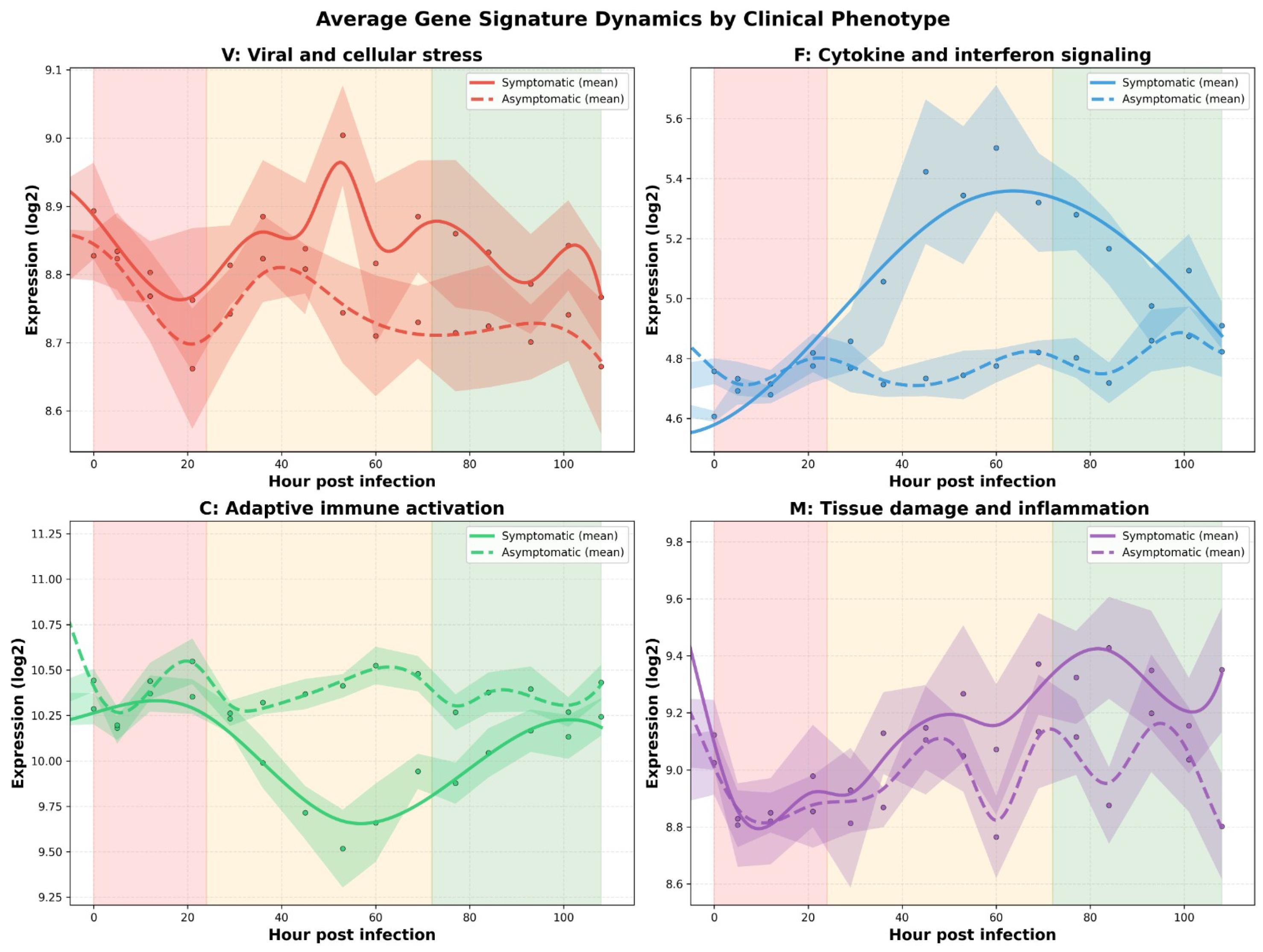
Before proceeding to parameter identification, we first examine the empirical dynamics of the aggregated transcriptomic signatures underlying the model. Figure 2 shows the averaged temporal evolution of the four latent states V ( t ) , F ( t ) , C ( t ) , and M ( t ) for symptomatic and asymptomatic patients, together with the corresponding ± 1 SEM bands.
Several qualitative differences between the two clinical phenotypes are immediately visible. The viral stress signature V ( t ) exhibits sustained growth and elevated levels in symptomatic patients, whereas in asymptomatic individuals it remains comparatively stable and shows signs of suppression at later time points. In contrast, the innate immune response F ( t ) displays a pronounced delayed peak in symptomatic patients, while remaining smoother and less amplified in asymptomatic cases. The adaptive immune activation C ( t ) further highlights this divergence: asymptomatic patients demonstrate partial recovery toward baseline levels, whereas symptomatic patients show persistent deviation, indicating a failure of stabilization. Finally, the tissue damage signature M ( t ) exhibits substantial variability in both groups, with wide SEM intervals, suggesting weak direct observability and limited identifiability from transcriptomic data alone.
These phenotype-dependent differences are not imposed by the model but arise directly from the data. As shown in the following subsections, they provide a structural explanation for the distinct parameter regimes obtained during identification, including the emergence of delayed interactions, the necessity of additional background terms, and the differential reliability of parameter estimates across subsystems.

5.1. Asymptomatic Basic Results

We calculate the coefficients from Formula (1) for transcriptomic latent states V ( t ) and F ( t ) :
d V d t = α 1 V ( t ) α 2 V ( t ) F ( t ) .
According to Formula (14), we proceed by Python [33] programming codes and obtain the desired coefficients in (35):
d V d t = 2.0 × 10 3 V ( t ) 4 . 410 4 V ( t ) F ( t ) .
Until all coefficients have acceptable relative accuracy
α 1 = 2.005036 × 10 3 ± 3.08 × 10 4 ( r e l . e r r = 15.38 % )
α 2 = 4.444098 × 10 4 ± 6.46 × 10 5 ( r e l . e r r = 14.53 % ) ,
and the problem is well-conditioned, the goodness of fit quantified by (30) equals R 2 = 0.2188 , so the final conclusion is that the identification of the right-hand side in (36) is not entirely reliable.
Analogously, we consider Formula (15) for the transcriptomic latent states C ( t ) , V ( t ) and F ( t ) , and we have:
d F d t = α 4 ( C ( t ) F ( t ) ) α 8 V ( t ) F ( t ) .
According to Formula (15), we proceed by Python programming codes and obtain the desired coefficients in (39):
d F d t = 1.4 × 10 2 ( C ( t ) F ( t ) ) + 1.9 × 10 3 V ( t ) F ( t ) .
This time all coefficients have acceptable relative accuracy
α 4 = 1.400518 × 10 2 ± 9.84 × 10 5 ( r e l . e r r = 0.70 % )
α 8 = 1.908441 × 10 3 ± 1.32 × 10 5 ( r e l . e r r = 0.69 % ) ,
and the problem is well-conditioned. Moreover, the goodness of fit quantified by (30) equals R 2 = 0.9912 , so the identification of the right-hand side in (40) is reliable. Finally, the condition number of the unregularized normal matrix calculated by (34) is κ = 3.676 × 10 4 , and the residual variance defined in (31) equals σ ^ 2 = 7.255 × 10 9 .
Next we take Formula (17) without delay setting τ = 0 for the transcriptomic latent states C ( t ) , V ( t ) and F ( t ) , and we have:
d C d t = α 3 V ( t ) F ( t ) α 5 ( C ( t ) 1 ) .
According to (18), we proceed, and obtain the coefficients in (43):
d F d t = 1.5 × 10 4 V ( t ) F ( t ) 7.0 × 10 4 ( C ( t ) 1 ) .
This time no coefficient has acceptable accuracy, since one or more coefficients are poorly determined:
α 3 = 1.505155 × 10 4 ± 3.95 × 10 4 ( r e l . e r r = 262.17 % )
α 5 = 6.984778 × 10 4 ± 1.76 × 10 3 ( r e l . e r r = 251.39 % )
The goodness of fit R 2 = 0.0007 , so the coefficient estimation in (44) is not reliable at all. The condition number κ = 1.840 × 10 5 , so it is still well-conditioned.
Finally, for (4), for the transcriptomic latent states V ( t ) and m ( t ) , we have:
d M d t = α 6 V ( t ) α 7 M ( t ) .
According to (16), we proceed, and obtain the coefficients in (47):
d M d t = 1.25 × 10 2 V ( t ) 1.21 × 10 2 M ( t ) .
This is not as high as before, but now the coefficient accuracy is not acceptable, since r e l . e r r 20 % :
α 6 = 1.245491 × 10 2 ± 2.79 × 10 3 ( r e l . e r r = 22.41 % )
α 7 = 1.210853 × 10 2 ± 2.72 × 10 3 ( r e l . e r r = 22.47 % )
The goodness of fit measure R 2 = 0.0998 , meaning that the coefficient estimation in (48) is not reliable. The condition number κ = 4.582 × 10 4 indicates good condition.

5.2. Symptomatic Basic Results

In this subsection we calculate coefficients for the patients with expressed symptoms. Again, first we calculate the coefficients from Formula (1) for transcriptomic latent states V ( t ) and F ( t ) :
d V d t = α 1 V ( t ) α 2 V ( t ) F ( t ) .
According to (14), we proceed with the programming codes and obtain the desired coefficients in (51):
d V d t = 1.5 × 10 3 V ( t ) 3.1 × 10 4 V ( t ) F ( t ) .
The coefficients have border accuracies
α 1 = 1.525295 × 10 3 ± 3.04 × 10 4 ( r e l . e r r = 19.92 % )
α 2 = 3.076068 × 10 4 ± 5.97 × 10 5 ( r e l . e r r = 19.40 % ) .
Until the problem is well-conditioned, since κ = 2 × 10 3 , the goodness of fit of R 2 = 0.1185 is not sufficient for entire reliability. Note that the coefficients are similar to those obtained in (35).
Analogously, Formula (2) gives, for C ( t ) , V ( t ) and F ( t ) :
d F d t = α 4 ( C ( t ) F ( t ) ) α 8 V ( t ) F ( t ) .
Formula (15) and the Python algorithm codes give:
d F d t = 1.8 × 10 2 ( C ( t ) F ( t ) ) 1.7 × 10 3 V ( t ) F ( t ) .
All coefficients have no acceptable relative accuracies
α 4 = 1.848495 × 10 3 ± 1.55 × 10 3 ( r e l . e r r = 84.02 % )
α 8 = 1.713092 × 10 4 ± 1.70 × 10 4 ( r e l . e r r = 99.47 % ) ,
and the goodness of fit equals R 2 = 0.0059 , so the identification of the right-hand side in (56) is not fully reliable. The condition κ = 2.458 × 10 2 calculated by (34) shows good conditioning, and residual variance σ ^ 2 = 1.918 × 10 4 .
Taking (17) without delay, with τ = 0 for the transcriptomic latent states C ( t ) , V ( t ) and F ( t ) , we have:
d C d t = α 3 V ( t ) F ( t ) α 5 ( C ( t ) 1 ) .
According to (18), we proceed, and obtain the coefficients in (43):
d C d t = 3.34 × 10 4 V ( t ) F ( t ) 1.60 × 10 3 ( C ( t ) 1 ) .
The coefficients are poorly determined:
α 3 = 3.340862 × 10 4 ± 2.96 × 10 4 ( r e l . e r r = 88.67 % )
α 5 = 1.602942 × 10 3 ± 1.48 × 10 3 ( r e l . e r r = 92.34 % )
The goodness of fit R 2 = 0.0065 shows no reliability at all, and the condition number κ = 9.187 × 10 2 is well-conditioned still. Compared to the symptomatic case, there is an evident deviation.
Applying (4) for the transcriptomic latent states V ( t ) and M ( t ) , we have:
d M d t = α 6 V ( t ) α 7 M ( t ) .
According to (16), we proceed, and obtain the coefficients in (63):
d M d t = 1.25 × 10 2 V ( t ) 1.21 × 10 2 M ( t ) .
This is not so high as before, but now the coefficient accuracy is not acceptable, since r e l . e r r 20 % :
α 6 = 1.114853 × 10 2 ± 2.00 × 10 3 ( r e l . e r r = 17.95 % )
α 7 = 1.043686 × 10 2 ± 1.93 × 10 3 ( r e l . e r r = 18.54 % )
The goodness of fit of R 2 = 0.1343 implies an unreliable coefficient estimation in (64). The condition number κ = 1.157 × 10 4 indicates good condition.

5.3. Asymptomatic Extended Model Results

In these two subsections we extend the model given from (1) to (4) with the mathematic tools presented in Section 4.6, and considering Section 4.4, where the values for τ are proposed in (27).
Since both (36) and (52) did not satisfy the reliability conditions with small R 2 values, we propose to extend (1) for latent states V ( t ) and F ( t ) with
d V d t = α 1 V ( t ) α 2 V ( t ) F ( t τ ) + γ 0 .
To obtain α 1 and α 2 in (67), we need to carry out as many iterations with as many τ that are suggested in (27). In Table 3 the iterations are sorted by WMSE, calculated in (28). Considering (7) and (8), we have different samples members’ numbers N t a u for calculating the coefficients. In Table 3, s d 1 and s d 2 are the weighted standard deviations used to normalize the regressors.
Finally we take α 1 , α 2 and γ obtained for τ = 0 , since in this case we have the smallest WMSE.
d V d t = 1.4 × 10 2 V ( t ) 3.8 × 10 3 V ( t ) F ( t ) + 2.8 × 10 1 .
The coefficients have definitely acceptable relative accuracies:
α 1 = 1.416189 × 10 2 ± 1.84 × 10 5 ( r e l . e r r 0.13 % )
α 2 = 3.778251 × 10 3 ± 3.98 × 10 6 ( r e l . e r r 0.11 % )
γ 0 = 2.805977 × 10 1 ± 3.08 × 10 4 ( r e l . e r r = 0.11 % )
In this case, R 2 = 0.9368 , condition κ = 7.819 , and residual variance σ ^ 2 = 5.3 × 10 9 , so the RHS identification is reliable indeed.
By comparing (67) with (36), it is shown that there is no delay in both cases. The need for the additional parameter γ 0 = 0.28 suggests that some biological processes occur that are not explicitly represented in the original structure of the model. The negative parameter in the case of viral population expansion in (68) is particularly interesting, as it indicates that something within the viral population causes extinction. First, we have only eight asymptomatic patients. It is possible that patients do not have disease symptoms precisely because of the negative coefficient α 1 .
Enlarging (2), with delay and an additional parameter assumption, we have
d F d t = α 4 ( C ( t τ ) F ( t ) ) α 8 V ( t τ ) F ( t ) + γ 0 .
Analyzing the coefficient fits for each τ value given in (27), we obtain Table 4.
From Table 4, we choose the coefficients given by τ = 0 again, because they give the smallest coefficient W M S E . We obtain the equation
d F d t = 1.7 × 10 2 ( C ( t ) F ( t ) ) + 1.6 × 10 3 V ( t ) F ( t ) + 2.9 × 10 2 .
The coefficients have acceptable relative accuracy:
α 4 = 1.701574 × 10 2 ± 5.06 × 10 5 ( r e l . e r r = 0.30 % )
α 8 = 1.625306 × 10 3 ± 1.12 × 10 5 ( r e l . e r r = 0.69 % )
γ 0 = 2.871100 × 10 2 ± 6.61 × 10 4 ( r e l . e r r = 2.30 % ) .
The coefficient of determination R 2 = 0.9991 shows that the regression model explains the variability of the dependent variable very well. The residual variance σ ^ 2 = 7.185993 × 10 10 implies very high model precision. After κ = 1.185 × 10 7 , the problem is moderately ill-conditioned, and caution is advised.
When we enlarge (17) for possible delays and an additional parameter, we get:
d C d t = α 3 V ( t τ ) F ( t τ ) α 5 ( C ( t ) 1 ) + γ 0 .
As before, calculating different τ from (27) entails τ = 0 , with the best W M S E , and the coefficients as follows:
d C d t = 1.1 × 10 3 V ( t ) F ( t ) 6.9 × 10 3 ( C ( t ) 1 ) + 1.1 × 10 1 .
In this case, we obtain coefficients with remarkable errors:
α 3 = 1.119225 × 10 3 ± 4.49 × 10 4 ( r e l . e r r = 40.07 % )
α 5 = 6.938193 × 10 3 ± 2.58 × 10 3 ( r e l . e r r = 37.24 % )
γ 0 = 1.121257 × 10 1 ± 2.92 × 10 2 ( r e l . e r r = 26.04 % ) .
Moreover, R 2 = 0.1218 shows that one or more coefficients are poorly determined. It is moderately ill-conditioned by κ = 4.062 × 10 6 , and RHS identification is not fully reliable until σ ^ 2 = 1.529 × 10 6 .
Related to (44), the coefficients in (78) are similar, and no delay is indicated. In particular, α 3 < 0 is very significant in the sense that this simple Marchuk model does not cover asymptomatic patients.
Particularly, if we want to consider (5)’s contribution to (77), then we need to enlarge our coefficient analysis.
d C d t = α 3 ζ ( m ) V ( t τ ) F ( t τ ) α 5 ( C ( t ) 1 ) ,
with ζ ( m ) defined just as in (5) somewhere above. In this case, we need a parallel τ and m discussion, presented in the following Table 5.
In Table 5 the best results are τ = 21 and m = 0.2 . In the sample created from N τ = 161 data by the spline given in (9), we obtain the immune activation differential equation
d C d t = 4.3 × 10 5 ζ ( m ) V ( t 21 ) F ( t 21 ) 1.1 × 10 4 ( C ( t ) 1 ) ,
with tissue damage function (5):
ζ ( m ) = 1 , 0 m < 0.2 , 1 m 1 0.2 , 0.2 m 1 .
Thanks to acceptable relative coefficient accuracies:
α 3 = 4.257395 × 10 5 ± 8.35 × 10 8 ( r e l . e r r = 0.20 % )
α 5 = 1.101979 × 10 4 ± 2.10 × 10 7 ( r e l . e r r = 0.19 % ) .
Together with the coefficients, from Table 5, the goodness of fit is R 2 = 0.9139 , condition number κ = 14.52 , and residual variance σ ^ 2 = 2.7 × 10 8 , guaranteeing the reliability of Equation (82)’s RHS identification.
Finally, transforming (4) to suppose a delay and taking an additional unused parameter for biological processes into account, we obtain the equation
d M d t = α 6 V ( t τ ) α 7 M ( t ) + γ 0 .
Different from above, now we get τ 0 through calculations, as presented in the next table.
From Table 6, sorted by the value of W M S E , we can find out the equation for the best τ = 21 h.
d M d t = 1.9 × 10 1 V ( t 21 ) + 3.6 × 10 2 M ( t ) 2.0 .
Considering (7) and (8), we have a sample of N t a u = 161 members for calculating coefficients with acceptable relative accuracies:
α 6 = 1.906749 × 10 1 ± 6.83 × 10 4 ( r e l . e r r = 0.36 % )
α 7 = 3.594986 × 10 2 ± 2.98 × 10 4 ( r e l . e r r = 0.83 % )
γ 0 = 1.992216 ± 8.01 × 10 3 ( r e l . e r r = 0.40 % )
The high goodness of fit is given by R 2 = 0.9395 , and the good predictive accuracy is given by σ ^ 2 = 9.535542 × 10 7 . However, caution is advised since κ = 3.035 × 10 6 , so the problem is moderately ill-conditioned.
The negative α 7 coefficient indicates tissue’s tendency to ruin itself in the absence of a cure, since there are no symptoms.

5.4. Symptomatic Model Extension Results

Patients with explicit symptoms show different behaviors from the first Equation (67). In contrast, we get contrasting results after analyzing τ cases. After sorting by WMSE, from Table 7, we obtain the optimal τ = 21 h.
For symptomatic patients, Equation (68) now reads as
d V d t = 3.9 × 10 2 V ( t ) 5.7 × 10 4 V ( t ) F ( t 21 ) 3.2 × 10 1 .
Both coefficients have acceptable relative accuracy:
α 1 = 3.939688 × 10 2 ± 1.60 × 10 5 ( r e l . e r r = 0.04 % )
α 2 = 5.707080 × 10 4 ± 2.01 × 10 7 ( r e l . e r r = 0.04 % )
γ 0 = 3.236927 × 10 1 ± 1.46 × 10 4 ( r e l . e r r = 0.05 % )
Good fitting is implied by R 2 = 0.9986 , and good conditioning by κ = 2.372 . Additionally, σ ^ 2 = 3.949807 × 10 9 , and RHS identification is reliable.
Related to (68), symptomatic patients have a positive virus propagation coefficient, as expected, so this might have caused their symptoms.
Considering (72) for the patient with symptoms, again we discuss the results for the different τ values proposed in (27).
In contrast with Table 7, the τ column in Table 8 is not ordered the same way, but the best is still τ = 21 h. For patients with symptoms, Equation (73) turns into
d F d t = 1.1 × 10 1 ( C ( t 21 ) F ( t ) ) + 1.9 × 10 2 V ( t 21 ) F ( t ) 1.4 .
Over the N τ = 161 data created, all coefficients α 4 , α 8 , and γ 0 have acceptable relative accuracies:
α 4 = 1.071965 × 10 1 ± 4.72 × 10 4 , ( r e l . e r r = 0.44 % )
α 8 = 1.916768 × 10 2 ± 9.17 × 10 5 ( r e l . e r r = 0.48 % )
γ 0 = 1.394323 ± 6.28 × 10 3 ( r e l . e r r = 0.45 % ) .
Finally we conclude that RHS identification is reliable, since high determination fixes the goodness of fit at R 2 = 0.9965 , the well condition number at κ = 4.067 × 10 4 , and small residual variance at σ ^ 2 = 7.472813 × 10 7 .
When relating (96) with (73), it is noticeable that in patients with symptoms, there is a positive cytokine dynamic dependence on surplus in adaptive immune activation in delay, in contrast with patients without symptoms. Meanwhile, the cytokines increase following their struggle with viruses in both cases.
Next, we find out the adaptive immune activation behavior when patients have disease symptoms. In this case, (78) become
d C d t = 5.2 × 10 3 V ( t 21 ) F ( t 21 ) + 4.7 × 10 2 ( C ( t ) 1 ) 6.6 × 10 1 ,
since the best τ = 21 after we sort the coefficient calculations by R 2 in Table 9.
Coefficient relative accuracies are obviously acceptable:
α 3 = 5.179970 × 10 3 ± 1.78 × 10 5 ( r e l . e r r = 0.34 % )
α 5 = 4.746952 × 10 2 ± 2.69 × 10 4 ( r e l . e r r = 0.57 % )
γ 0 = 6.560232 × 10 1 ± 2.64 × 10 3 ( r e l . e r r = 0.40 % ) .
The final conclusion is that RHS identification is reliable, which is a consequence of high determination, R 2 = 0.9985 and good conditioning, κ = 2.464 × 10 4 , and strictness, σ ^ 2 = 2.530 × 10 7 .
The patients have symptoms since there is a delay in the body’s reaction. In contrast to (78), here, the immune reaction increases with the struggle between cytokines and viruses, with higher immune activity.
A tissue damage and inflammation impact in (100) is obtained by calculating the coefficients in (82). Similarly to Table 5, we use Table 10.
From Table 5, the immune activation equation reads
d C d t = 6.0 × 10 4 ζ ( m ) V ( t ) F ( t ) + 1.8 × 10 3 ( C ( t ) 1 ) ,
with tissue damage behavior
ζ ( m ) = 1 , 0 m < 0.4 , 1 m 1 0.4 , 0.4 m 1 .
This is obtained for the best choice τ = 0 and m = 0.4 from the sample created from N 0 = 200 items. The coefficients
α 3 = 6.016994 × 10 4 ± 2.86 × 10 6 ( r e l . e r r = 0.48 % ) , and
α 5 = 1.831814 × 10 3 ± 1.06 × 10 5 ( r e l . e r r = 0.58 % )
are of acceptable relative accuracies. The fit goodness is R 2 = 0.7145 , along with an acceptable condition number κ = 13.7 and suitable residual variance σ ^ 2 = 4.094621 × 10 5 , implying that RHS identification is reliable.
If we relate (104) to asymptomatic (104), we recognize symptom absence by increasing the immune activity with the increasing struggle with viruses after 21 days. In contrast, patients with symptoms lose immune activity in the struggle and get immunity from an increase in cell density in the blood.
Finally, we calculate the coefficients in (87) for patients with symptoms. The τ grid results are sorted by WMSE in Table 11.
The best τ = 5.0 choice leads to a sample with N 5 = 190 items and gives the equation
d M d t = 2.2 × 10 1 V ( t 5 ) 2.0 × 10 2 M ( t ) 1.8
with acceptable relative accuracies
α 6 = 2.247493 × 10 1 ± 3.20 × 10 4 ( r e l . e r r = 0.14 % )
α 7 = 1.981986 × 10 2 ± 4.01 × 10 1 ( r e l . e r r = 0.20 % )
γ 0 = 1.803576 ± 2.70 × 10 1 ( r e l . e r r = 0.15 % )
Once more, the determination coefficient R 2 = 0.9911 is high and residual variance σ ^ 2 = 2.257807 × 10 7 indicates high dependence on residuals. But, the condition number κ = 1.216 × 10 6 warrants caution of moderately ill-conditioned RHS identification, since it is not fully reliable.
Unlike asymptomatic patients, symptomatic patients take medication that helps keep tissues out of the risk zone defined by (5).

6. Conclusions

This study examined the identifiability of parameters in a Marchuk-type immune response model using aggregated transcriptomic gene-signature time series derived from the dataset G S E 30550 . The primary objective was to determine which subsystems of the model can be reliably calibrated from transcriptomic observations and which remain weakly constrained due to structural or informational limitations.
The results demonstrate that the parameters governing viral dynamics and the innate immune response are consistently identifiable. In particular, the viral growth and suppression coefficients in the V ( t ) equation, as well as the interaction terms in the F ( t ) equation, exhibit low relative errors, stable numerical conditioning, and high goodness-of-fit values. These parameters can therefore be interpreted as effective interaction rates within a reduced transcriptomic state-space representation.
In contrast, the adaptive immune response C ( t ) and tissue damage dynamics M ( t ) are inadequately characterized within the classical model framework. Although the associated regression problems are numerically optimized, these equations yield low coefficients of determination and high relative uncertainties. This points to a structural, rather than data-driven, limitation: transcriptomic signatures alone do not sufficiently constrain adaptive immunity and tissue damage without additional modeling assumptions.
Model extensions significantly improve identifiability. The introduction of an additive background term γ 0 leads to a substantial reduction in residual variance and stabilizes parameter estimates across multiple subsystems. This behavior indicates the presence of systematic background processes or unobserved regulatory mechanisms not captured by the classical formulation. From a modeling perspective, γ 0 acts as a structural correction rather than as a numerical artifact.
Clear differences are observed between asymptomatic and symptomatic patients. Asymptomatic dynamics are generally associated with negligible delay effects, while symptomatic cases consistently favor delayed regulation, with a characteristic delay of approximately 21 h. This delay appears in several equations and points to fundamentally different immune response regimes between the two clinical phenotypes.
Finally, incorporating tissue damage modulation through the function ζ ( m ) restores reliable identifiability for the adaptive immune equation in asymptomatic patients. This extension results in improved goodness-of-fit, reduced parameter uncertainty, and well-conditioned regression problems, emphasizing the importance of tissue state in regulating adaptive immune activation.
These findings indicate that aggregated transcriptomic data are sufficient to identify well-observed subsystems of immune–virus interaction models but are insufficient for classical formulations of adaptive immunity and tissue damage. Reliable parameter identification requires explicit inclusion of background processes, tissue-dependent regulation, and phenotype-specific delays. This explains why classical immune response models often fail when applied directly to transcriptomic data and provides concrete guidance for constructing structurally identifiable models in future studies.
We emphasize that the estimated coefficients characterize the specific cohort and viral strain of the GSE30550 dataset and are not intended as universal biological constants. The primary transferable contribution of this work is the identification methodology itself: the pipeline for deriving structurally interpretable parameters from transcriptomic latent states, which can be applied to other datasets with appropriate re-identification.
We used the Marchuk discrete-delay model primarily for reasons of interpretability and identifiability: its four-state structure maps naturally to our transcriptomic signatures, and the linear-in-parameters form enables stable estimation from a small, irregular cohort using smoothing plus ridge regularization. We acknowledge that the biological immune response likely depends on a continuum of past states and that distributed-delay formulations can be more realistic [13]. Fitting such integral models typically requires denser sampling, alternative numerical schemes, and stronger prior or hierarchical assumptions to ensure identifiability ingredients that were not available in the present single-cohort study. Investigation of distributed delays and integral estimation methods is an important direction planned for future work when richer longitudinal datasets become available.

Author Contributions

Conceptualization, M.B.; software, validation, G.K.; formal analysis, M.B.; writing—original draft preparation, M.B.; writing—review and editing, visualization G.K. All authors have read and agreed to the published version of the manuscript.

Funding

This research received no external funding.

Data Availability Statement

In this study, we used the publicly available transcriptomic dataset G S E 30550 , https://www.ncbi.nlm.nih.gov/geo/query/acc.cgi?acc=GSE30550, (accessed on 31 December 2025) obtained from Gene Expression Omnibus (GEO) [2].

Acknowledgments

The authors thank Boris Krasovitov for valuable discussions during the preparation of this manuscript.

Conflicts of Interest

The authors declare no conflicts of interest.

References

  1. Zuev, S.M. Statistical Evaluation of Parameters of Mathematical Models of Diseases; Nauka: Moscow, Russia, 1988. [Google Scholar]
  2. Huang, Y.; Zaas, A.K.; Rao, A.; Dobigeon, N.; Woolf, P.J.; Veldman, T.; Ien, N.C.; McClain, M.T.; Varkey, J.B.; Nicholson, B.; et al. Temporal dynamics of host molecular responses differentiate symptomatic and asymptomatic influenza a infection. PLoS Genet. 2011, 7, e1002234. Available online: https://www.ncbi.nlm.nih.gov/geo/query/acc.cgi?acc=GSE30550 (accessed on 20 November 2025). [CrossRef] [Scilit] [PubMed]
  3. Chaussabel, D.; Baldwin, N. Democratizing systems immunology with modular transcriptional repertoire analyses. Nat. Rev. Immunol. 2014, 14, 271–280. [Google Scholar] [CrossRef] [Scilit] [PubMed]
  4. Domoshnitsky, A.; Bershadsky, M.; Volinsky, I. Distributed control in stabilization of a model of infection diseases. Russ. J. Biomech. 2019, 23, 579–585. [Google Scholar] [CrossRef] [Scilit]
  5. Foryś, U. Marchuk’s model of immune system dynamics with application to tumour growth. J. Theor. Med. 2002, 4, 85–93. [Google Scholar] [CrossRef] [Scilit]
  6. Subramanian, A.; Tamayo, P.; Mootha, V.K.; Tamayo, P.; Mukherjee, S.; Ebert, B.L.; Gillette, M.A.; Paulovich, A.; Pomeroy, S.L.; Golub, T.R.; et al. Gene set enrichment analysis: A knowledgebased approach for interpreting genome-wide expression profiles. Proc. Natl. Acad. Sci. USA 2005, 102, 15545–15550. [Google Scholar]
  7. Mazel-Sanchez, B.; Iwaszkiewicz, J.; Bonifacio, J.P.P.; Silva, F.; Niu, C.; Strohmeier, S.; Eletto, D.; Krammer, F.; Tan, G.; Zoete, V.; et al. Influenza A viruses balance ER stress with host protein synthesis shutoff. Proc. Natl. Acad. Sci. USA 2021, 118, e2024681118. [Google Scholar] [CrossRef] [Scilit]
  8. Shapira, S.D.; Gat-Viks, I.; Shum, B.O.V.; Dricot, A.; de Grace, M.M.; Wu, L.; Gupta, P.B.; Hao, T.; Silver, S.J.; Root, D.E.; et al. A physical and regulatory map of host-influenza interactions reveals pathways in H1N1 infection. Cell 2009, 139, 1255–1267. [Google Scholar] [CrossRef] [Scilit]
  9. McNab, F.; Mayer-Barber, K.; Sher, A.; Wack, A.; O’garra, A. Type I interferons in infectious disease. Nat. Rev. Immunol. 2015, 15, 87–103. [Google Scholar] [CrossRef] [Scilit]
  10. Huang, M.; Xu, R.; Triffon, C.; Mifsud, N.; Chen, W. Broad-Based Influenza-Specific CD8+ T Cell Response without the Typical Immunodominance Hierarchy and Its Potential Implication. Viruses 2021, 13, 1080. [Google Scholar] [CrossRef] [Scilit]
  11. Tang, B.M.; Shojaei, M.; Teoh, S.; Meyers, A.; Ho, J.; Ball, T.B.; Keynan, Y.; Pisipati, A.; Kumar, A.; Eisen, D.P.; et al. Neutrophils-related host factors associated with severe disease and fatality in patients with influenza infection. Nat. Commun. 2019, 10, 3422. [Google Scholar] [CrossRef] [Scilit]
  12. Rojas-Quintero, J.; Wang, X.; Tipper, J.; Burkett, P.R.; Zuñiga, J.; Ashtekar, A.R.; Polverino, F.; Rout, A.; Yambayev, I.; Hernández, C.; et al. Matrix metalloproteinase-9 deficiency protects mice from severe influenza A viral infection. JCI Insight 2018, 3, e99022. [Google Scholar] [CrossRef] [Scilit]
  13. Seok, J.; Warren, H.S.; Cuenca, A.G.; Mindrinos, M.N.; Baker, H.V.; Xu, W.; Richards, D.R.; McDonald-Smith, G.P.; Gao, H.; Hennessy, L.; et al. Genomic responses in mouse models poorly mimic human inflammatory diseases. Proc. Natl. Acad. Sci. USA 2013, 110, 3507–3512. [Google Scholar] [CrossRef] [Scilit]
  14. Marchuk, G.I. Mathematical Modelling of Immune Response in Infectious Diseases; Springer Science: Berlin/Heidelberg, Germany, 1997; Volume 395. [Google Scholar]
  15. Marchuk, G.I.; Petrov, R.V.; Romanyukha, A.A.; Bocharov, G.A. Mathematical model of antiviral immune response. I. Data analysis, generalized picture construction and parameters evaluation for hepatitis B. J. Theor. Biol. 1997, 151, 1–40. [Google Scholar] [CrossRef] [Scilit] [PubMed]
  16. Volinsky, I.; Domoshnitsky, A.; Bershadsky, M.; Shklyar, R. Marchuk’s models of infection diseases: New developments in Functional Differential Equations and Applications. In International Workshop on Functional Differential Equations and Applications; Springer: Berlin/Heidelberg, Germany, 2020; p. 379. [Google Scholar]
  17. Bershadsky, M.; Chirkov, M.; Domoshnitsky, A.; Rusakov, S.; Volinsky, I. Distributed control and the Lyapunov characteristic exponents in the model of infectious diseases. Complexity 2019, 2019, 5234854. [Google Scholar] [CrossRef] [Scilit]
  18. Volinsky, I.; Bershadsky, M. Numerical Solution of Marchuk Model of Infection Diseases. Funct. Differ. Equ. 2021, 28, 85–93. [Google Scholar] [CrossRef] [Scilit]
  19. Liţcanu, G. A brief look at the mathematical modelling of the immune response. Analele ŞTiinţifice Ale Univ. Cuza’Din Iaşi. Mat. (New Ser.) 2020, 66, 289–300. [Google Scholar]
  20. Brunton, S.L.; Proctor, J.L.; Kutz, J.N. Discovering governing equations from data by sparse identification of nonlinear dynamical systems. Proc. Natl. Acad. Sci. USA 2016, 113, 3932–3937. [Google Scholar] [CrossRef] [Scilit]
  21. Bellen, A.; Zennaro, M. Numerical Methods for Delay Differential Equations; OUP: Oxford, UK, 2003. [Google Scholar]
  22. Adomian, G.; Adomian, G.E. Solution of the Marchuk Model of Infectious Disease and Immune Response. Math. Model. 1986, 7, 803–807. [Google Scholar] [CrossRef] [Scilit]
  23. Ramsay, J.O.; Hooker, G.; Campbell, D.; Cao, J. Parameter estimation for differential equations: A generalized smoothing approach. J. R. Stat. Soc. Ser. Stat. Methodol. 2007, 69, 741–796. [Google Scholar] [CrossRef] [Scilit]
  24. Brunel, N.J. Parameter estimation of ODE’s via nonparametric estimators. Electron. J. Stat. 2008, 2, 1242–12467. [Google Scholar] [CrossRef] [Scilit]
  25. Gugushvili, S.; Klaassen, C.A.J. n-consistent parameter estimation for systems of ordinary differential equations: Bypassing numerical integration via smoothing. arXiv 2010, arXiv:1007.3880. [Google Scholar] [CrossRef] [Scilit]
  26. Baker, C.T.H.; Bocharov, G.A. Computational Aspects of Time-Lag Models of Marchuk Type That Arise in Immunology. Russ. J. Numer. Anal. Math. Model. 2005, 20, 247–262. [Google Scholar] [CrossRef]
  27. Villaverde, A.F.; Barreiro, A.; Papachristodoulou, A. Structural identifiability of dynamic systems biology models. PLoS Comput. Biol. 2016, 12, e1005153. [Google Scholar] [CrossRef] [Scilit] [PubMed]
  28. Ivan, F.X.; Tan, K.S.; Phoon, M.C.; Engelward, B.P.; Welsch, R.E.; Rajapakse, J.C.; Chow, V.T. Neutrophils infected with highly virulent influenza H3N2 virus exhibit augmented early cell death and rapid induction of type I interferon signaling pathways. Genomics 2013, 101, 101–112. [Google Scholar] [CrossRef] [Scilit] [PubMed]
  29. Baccam, P.; Beauchemin, C.; Macken, C.A.; Hayden, F.G.; Perelson, A.S. Kinetics of influenza A virus infection in humans. J. Virol. 2006, 80, 7590–7599. [Google Scholar] [CrossRef] [Scilit] [PubMed]
  30. Smith, A.M.; Perelson, A.S. Influenza A virus infection kinetics: Quantitative data and models. Wiley Interdiscip. Rev. Syst. Biol. Med. 2011, 3, 429–445. [Google Scholar] [CrossRef] [Scilit]
  31. Belz, G.T.; Xie, W.; Doherty, P.C. Diversity of epitope and cytokine profiles for primary and secondary influenza a virus-specific CD8+ T cell responses. J. Immunol. 2001, 166, 4627–4633. [Google Scholar] [CrossRef] [Scilit]
  32. Simpkins, A. System identification: Theory for the user, (ljung, l.; 1999) [on the shelf]. IEEE Robot. Autom. Mag. 2012, 19, 95–96. [Google Scholar] [CrossRef] [Scilit]
  33. Python 3 version. Available online: https://www.google.com/search?q=Python+3.10.12&oq=Python+3.10.12&gs_lcrp=EgZjaHJvbWUqBggAEEUYOzIGCAAQRRg (accessed on 31 December 2025).
Figure 1. End-to-end parameter identification pipeline consists of six phases.
Computation 14 00108 g001
Figure 2. Average gene signature dynamics by clinical phenotype.
Computation 14 00108 g002
Table 1. GSE30550 dataset properties and constraints for data-driven immune system modeling.
AspectValueImplications for Mathematical Modeling
Study designHuman influenza challenge studyControlled viral exposure enables causal interpretation of temporal dynamics
Virus strainInfluenza A/H3N2 (A/Wisconsin/67/2005)Supports modeling of acute respiratory viral infection
PlatformAffymetrix Human Genome U133A 2.0 ArrayMicroarray-based expression with limited dynamic range
Biological materialWhole peripheral bloodSignals reflect mixed immune cell populations rather than tissue-specific processes
Number of subjects17Small cohort size; inter-individual variability dominates population averages
Clinical phenotypesSymptomatic ( n = 9 ) vs. asymptomatic ( n = 8 )Enables comparative structural analysis of immune response dynamics
Temporal resolutionUp to 108 h post-infection, irregular samplingContinuous-time differential equation models are preferred
Feature dimensionality∼20,000 genesRequires dimensionality reduction via biologically informed gene signatures
Total samples268 transcriptomic profilesInsufficient for direct high-dimensional system identification
Expression value rangeMin: 2.99, Median: 6.76,
Max: 15.11
Log-scale stabilized expression supports linear regression assumptions
Table 2. Biological gene signatures used for state construction.
SignatureBiological ProcessInterpretation in the ModelRepresentative Genes
VViral and cellular stressProxy for viral activity and host stress responseHSPA5, HSP90B1, DDIT3, ATF4, ATF6, XBP1, ERN1, EDEM1, HERPUD1, DNAJB9, PPP1R15A, PDIA4, PDIA6, HMOX1, SOD2, TXN, TXNRD1, NQO1, GCLM, GCLC, PRDX1, SLC2A1, HK2, PFKP, ALDOA, ENO1, LDHA, PDK1, BNIP3, JUN, FOS, ATF3, EGR1
FCytokine and interferon signalingIntensity of innate immune activationIFNB1, IL1A, IL1B, IL18, IL6, TNF, IFNG, CXCL8, CXCL10, CCL2, CCL4, CCL5
CAdaptive immune activationT cell-mediated immune response strengthCD3D, CD3E, CD3G, CD4, CD8A, CD8B, IL7R, TCF7, PRF1, GZMB, NKG7, CD69, CD2
MTissue damage and inflammationDegree of immunopathologyS100A8, S100A9, S100A12, LCN2, ELANE, MPO, AZU1, CTSG, MMP8, MMP9, CEACAM8, CD14, LST1, ITGAM, CD68, CSF1R, CD163, SERPINE1
Table 3. Differential Equation (67)’s coefficients calculated for the proposed delay values τ .
τ N τ α 1 α 2 γ 0 R 2 RMSE WMSE sd 1 sd 2
0.0200−0.0141620.0037780.2805980.9367860.000077 5.282461 × 10 9 0.0280970.130065
5.0190−0.0111340.0044590.2823820.9062820.000089 7.610578 × 10 9 0.0247710.101021
12.0177−0.0052350.0054150.2704130.8430120.000113 1.174103 × 10 8 0.0224680.063693
21.01610.0059610.0045430.1360080.7496650.000147 1.755012 × 10 8 0.0210060.028084
Table 4. Differential Equation (72)’s coefficients calculated for the asymptomatic patients from the delays τ proposed in (27).
τ N τ α 4 α 8 γ 0 R 2 RMSE WMSE
0.0200−0.017016−0.0016250.0287110.9991280.000027 7.972498 × 10 10
5.0190−0.012940−0.002802−0.0433870.9802560.000130 1.910559 × 10 8
21.01610.017478−0.009085−0.4771500.9569750.000202 3.915370 × 10 8
12.0177−0.000151−0.005826−0.2416350.9475340.000218 4.840645 × 10 8
Table 5. Equation (82)’s coefficients calculated considering delay τ , and healthy tissue m from (5), sorted by WMSE.
τ m N τ α 3 α 5 R 2 RMSEWMSE κ σ ^ 2
21.00.21610.0000430.0001100.9139020.0001832.670078 × 10 8 14.5223312.670332 × 10 8
21.00.31610.0000380.0001110.8742410.0002223.844297 × 10 8 13.5511983.844663 × 10 8
21.00.41610.0000350.0001120.8176070.0002675.967419 × 10 8 13.5069905.967987 × 10 8
21.00.51610.0000330.0001130.7475020.0003148.788103 × 10 8 14.2594848.788939 × 10 8
12.00.21770.0000500.0001190.8334480.0003559.439431 × 10 8 14.0694169.440279 × 10 8
21.00.61610.0000310.0001140.6641400.0003621.221799 × 10 7 15.7367891.221916 × 10 7
12.00.31770.0000450.0001180.7674030.0004191.307994 × 10 7 13.6879001.308112 × 10 7
21.00.71610.0000280.0001140.5660810.0004111.647659 × 10 7 18.0342671.647816 × 10 7
12.00.41770.0000410.0001180.6958380.0004791.739119 × 10 7 13.9590661.739275 × 10 7
21.00.81610.0000260.0001120.4499930.0004632.087612 × 10 7 21.6487492.087811 × 10 7
12.00.51770.0000380.0001190.6209890.0005352.208412 × 10 7 14.9250532.208610 × 10 7
5.00.21900.0000590.0001300.7701940.0005312.387549 × 10 7 13.9698812.387752 × 10 7
12.00.61770.0000360.0001190.5411790.0005892.722144 × 10 7 16.5951672.722389 × 10 7
5.00.31900.0000530.0001280.6972170.0006093.130792 × 10 7 13.9636573.131058 × 10 7
12.00.71770.0000330.0001180.4531200.0006433.321400 × 10 7 19.1108363.321698 × 10 7
5.00.41900.0000480.0001270.6228510.0006803.894349 × 10 7 14.4772493.894680 × 10 7
12.00.81770.0000300.0001160.3567200.0006973.916946 × 10 7 22.9953003.917298 × 10 7
5.00.51900.0000450.0001260.5487500.0007444.644770 × 10 7 15.6254114.645165 × 10 7
0.00.22000.0000710.0001440.7357290.0006735.090517 × 10 7 14.0919575.090922 × 10 7
5.00.61900.0000420.0001260.4728530.0008045.412176 × 10 7 17.4722415.412636 × 10 7
5.00.71900.0000380.0001240.3916020.0008646.266664 × 10 7 20.1961806.267197 × 10 7
0.00.32000.0000640.0001410.6655590.0007576.458883 × 10 7 14.4238166.459397 × 10 7
5.00.81900.0000350.0001200.3054140.0009237.089489 × 10 7 24.3452767.090091 × 10 7
0.00.42000.0000590.0001390.5942100.0008347.774117 × 10 7 15.1830267.774736 × 10 7
0.00.52000.0000550.0001370.5228110.0009058.991271 × 10 7 16.5337438.991987 × 10 7
0.00.62000.0000510.0001350.4500170.0009711.017902 × 10 6 18.5891621.017983 × 10 6
0.00.72000.0000470.0001310.3731280.0010371.145564 × 10 6 21.5669201.145655 × 10 6
0.00.82000.0000430.0001260.2911970.0011021.265375 × 10 6 26.0452171.265475 × 10 6
Table 6. Differential Equation (87)’s coefficients calculated for the proposed delays τ .
τ N τ α 6 α 7 γ 0 R 2 RMSE WMSE
21.01610.190675−0.035950−1.9922160.9394590.0009679.036256 × 10−7
12.01770.166507−0.039713−1.8132540.8823890.0012992.109007 × 10−6
5.01900.143496−0.040383−1.6171160.8047050.0016172.937014 × 10−6
0.02000.126178−0.038358−1.4469330.7284240.0018623.624937 × 10−6
Table 7. DifferentialEquation (67)’s coefficients calculated for symptomatic patients.
τ N τ α 1 α 2 γ 0 R 2 RMSEWMSE sd 1 sd 2
21.01610.0393970.000571−0.3236930.9986400.000066 3.949315 × 10 9 0.0276242.209233
12.01770.0531460.000680−0.4401110.9981580.000078 7.197558 × 10 9 0.0262452.154433
5.01900.0735620.000872−0.6118490.9970960.000098 1.067946 × 10 8 0.0252162.200710
0.02000.1027850.001158−0.8573380.9953620.000123 1.577989 × 10 8 0.0251812.165551
Table 8. Differential Equation (72)’s coefficients calculated for symptomatic patients using the delays, τ , proposed in (27), sorted by WMSE.
τ N τ α 4 α 8 γ 0 R 2 RMSEWMSE
21.01610.107196−0.019168−1.3943230.9965270.000856 4.922686 × 10 7
12.01770.184169−0.034240−2.4493380.9924240.001251 1.145468 × 10 6
0.0200−0.3947930.0747245.3086690.9410210.003356 9.490120 × 10 6
5.01900.648089−0.122347−8.6978040.9031360.004386 1.531430 × 10 5
Table 9. Differential Equation (77)’s coefficients calculated for symptomatic patients considering the delays, τ , proposed in (27), and sorted by R 2 .
τ N τ α 3 α 5 γ 0 R 2 κ σ ^ 2
211610.005180−0.047470−0.6560230.99853124644.220169 2.529854 × 10 7
121770.006758−0.071319−0.9440370.99627937619.395502 6.284911 × 10 7
51900.009965−0.113021−1.4656260.97854891743.724943 3.495866 × 10 6
02000.014135−0.165637−2.1283350.790921443416.244682 3.281703 × 10 5
Table 10. Equation (82)’s calculated coefficients taking into account delays, τ , and tissue health, m , for symptomatic patients, sorted by WMSE, and additionally by R 2 .
τ m N τ α 3 α 5 R 2 RMSEWMSE κ σ ^ 2
0.00.4200−0.000602−0.0018320.7145220.0066440.00004113.6958930.000041
0.00.3200−0.000596−0.0017660.6965110.0068500.00004112.9696880.000041
0.00.5200−0.000610−0.0019090.7204850.0065740.00004214.7149340.000042
0.00.2200−0.000591−0.0017040.6709140.0071330.00004312.4064930.000043
0.00.6200−0.000621−0.0020060.7062570.0067390.00004416.2534320.000044
5.00.4190−0.000618−0.0018380.7085620.0068370.00004612.1918640.000046
5.00.3190−0.000614−0.0017720.6931460.0070150.00004711.5432110.000047
5.00.5190−0.000624−0.0019150.7116250.0068010.00004713.1184930.000047
5.00.2190−0.000613−0.0017120.6702030.0072730.00004811.0551400.000048
5.00.6190−0.000632−0.0020100.6937910.0070080.00005114.5242290.000051
0.00.7200−0.000629−0.0021180.6546590.0073070.00005118.7782910.000051
12.00.3177−0.000634−0.0017790.6794320.0072960.00005510.1108370.000055
12.00.4177−0.000633−0.0018440.6929500.0071410.00005510.6524100.000055
12.00.2177−0.000637−0.0017210.6588390.0075270.0000569.7372330.000056
12.00.5177−0.000636−0.0019190.6940650.0071280.00005611.4613630.000056
5.00.7190−0.000633−0.0021140.6375100.0076250.00006016.8136000.000060
12.00.6177−0.000639−0.0020100.6737580.0073600.00006112.7049560.000061
21.00.3161−0.000649−0.0017820.6476970.0077170.0000649.1460900.000064
21.00.4161−0.000642−0.0018430.6611770.0075680.0000649.5418570.000065
21.00.2161−0.000660−0.0017280.6284160.0079260.0000658.9562220.000065
21.00.5161−0.000638−0.0019150.6626470.0075520.00006710.2140820.000067
12.00.7177−0.000630−0.0021030.6140740.0080050.00007214.7068070.000072
21.00.6161−0.000634−0.0019990.6424090.0077750.00007211.2875480.000072
0.00.8200−0.000592−0.0021320.5198340.0086160.00007423.3014960.000074
21.00.7161−0.000612−0.0020760.5817640.0084080.00008512.9924450.000085
5.00.8190−0.000581−0.0020990.4963660.0089880.00008620.8034460.000086
12.00.8177−0.000556−0.0020510.4671200.0094070.00010318.0462030.000103
21.00.8161−0.000512−0.0019850.4297770.0098180.00011815.8665730.000118
Table 11. Calculated Equation (87) coefficients, sorted by WMSE.
τ N τ α 6 α 7 γ 0 R 2 RMSEWMSE
5.01900.2247490.019820−1.8035760.9911140.000471 2.546462 × 10 7
12.01770.2944150.038927−2.2448110.9835240.000654 4.087418 × 10 7
0.02000.1942820.008721−1.6355390.9783690.000743 6.703930 × 10 7
21.01610.3886240.069777−2.7942720.8278510.002214 4.648536 × 10 6
Disclaimer/Publisher’s Note: The statements, opinions and data contained in all publications are solely those of the individual author(s) and contributor(s) and not of MDPI and/or the editor(s). MDPI and/or the editor(s) disclaim responsibility for any injury to people or property resulting from any ideas, methods, instructions or products referred to in the content.