Comparative Analysis of Machine Learning Algorithms to Predict Municipal Solid Waste

Abstract

The management of municipal solid waste in intermediate cities exhibits high daily variability and source heterogeneity, which hinders operational sizing and material recovery. Reliable predictions are required from heterogeneous and often-scarce data. However, studies that compare multiple machine learning algorithms with temporal validation on short time series in intermediate cities are still limited. This study compares fourteen machine learning algorithms to predict the daily generation of organic and inorganic waste in La Joya de los Sachas, Ecuador, formulating the problem as a multi-output regression problem. An adapted CRISP-DM design was employed, using primary data from a waste characterization campaign, temporal feature engineering, variable encoding, and an expanding-window backtesting protocol against lag-7 persistence and ARIMA. Tree-based ensembles achieved the best performance. AdaBoost provided the best organic forecasts ($R^2$$=0.985$, $\mathrm{RMSE}$ $=0.081$, $\mathrm{MAE}$$=0.061$ in rate space), while Random Forest was best for inorganic ($R^2$$=0.965$, $\mathrm{RMSE}$ $=0.049$, $\mathrm{MAE}$$=0.040$). Linear models were stable but slightly inferior, and other approaches (SVR, KNN, MLP, Lasso, ElasticNet) showed lower generalization capacity. The study provides a multi-output regression protocol with temporal validation for municipal contexts with short time series, comparative evidence across fourteen algorithms, and a conversion from rates to kilograms for operational use.

1. Introduction

Municipal solid waste (MSW) management is a growing challenge in intermediate Latin American cities due to population growth, urban expansion, and variability in consumption habits [1]. These dynamics strain municipal MSW management systems—including collection, transport, treatment, and final disposal services—while exacerbating environmental impacts: pollutant emissions, leachate posing risks to soil and groundwater, and the accumulation of inorganic waste in non-sanitary sites [2].

In this context, La Joya de los Sachas presents a diversity of waste-generating sources—households, markets, commercial establishments, institutions, and street sweeping—that produce flows with differentiated compositions between organic and inorganic fractions. The municipality lacks a continuous, daily historical record disaggregated with sufficient detail, which increases operational uncertainty and makes it difficult to adjust routes, frequencies, and capacities [3]. Therefore, it is necessary to accurately estimate the daily generation of organic and inorganic waste to support decisions on collection, treatment, disposal, and recovery strategies [4], thus reducing pressure on the MSW system [5].

The literature reports econometric models [6], time series [7], and simulations [8], together with a growing adoption of machine learning (ML) algorithms [9]—regressions, decision trees, support vector machines, and neural networks—that capture nonlinear relationships and improve accuracy compared to traditional approaches [10]. Nevertheless, most studies assume large data volumes and report aggregated outputs [11]; therefore, comparative multi-algorithm studies under a homogeneous protocol are scarce when time series are short and data are heterogeneous [12].

In light of this, the following research question is posed: Which ML algorithm provides the best predictive performance to estimate daily organic and inorganic waste in La Joya de los Sachas?

To answer this question, the purpose of this article is to compare fourteen tabular ML algorithms for one-day-ahead forecasting of daily MSW generation disaggregated into organic and inorganic fractions in La Joya de los Sachas. We formulate the task as a multi-output regression problem because both fractions are measured jointly each day and share the same operational and temporal predictors. All models are evaluated under a homogeneous expanding-window temporal backtesting protocol with explicit autoregressive baselines and an operational conversion of predictions from rates to kilograms.

Related Work

ML is used to forecast MSW. Most studies use single-output models (total MSW or one fraction), monthly or yearly data, and long historical series. Table 1 summarizes representative works in this area.

Table 1. Representative studies on MSW forecasting using ML.

Study	City/Context	Temporal Resolution and Horizon	Series Length	Algorithms	Validation and Outputs
[13]	China (national level)	Annual MSW generation, medium–long-term scenarios	Several decades of historical data	Linear and polynomial regression, SVR, Random Forest, XGBoost	Train/test split without explicit temporal CV; single-output (total MSW).
[14]	Singapore	Annual MSW by category, 2003–2021 (waste audits for P&C, plastics, food)	19 years (2003–2016 train, 2017–2021 test)	k-Nearest Neighbors, SVR, ExtraTrees, CatBoost, XGBoost (GSO-XGBoost as optimized model)	Separate single-output models for three waste categories, no explicit multi-output formulation.
[15]	Multi-city (China)	City-level MSW, monthly/annual horizons	Multi-year time series for several cities	Gradient Boosting Regression Trees and other ML baselines	Hold-out validation by city and period; single-output, no explicit multi-output formulation.
[16]	Building-level MSW in New York City	Building-level generation (aggregated over time)	Multi-year administrative records	Ensemble ML models combined with small area estimation	Cross-validation over buildings; single-output per building.
[17]	Multiple cities (Australia, USA, Sri Lanka)	Daily MSW, multi-step forecasting	Long daily series (years) for five datasets	Random Forest, XGBoost, and other ML models, plus deep learning architectures (LSTM, TCN, etc.)	Mainly univariate or single-output setups, without fraction-specific multi-output regression.
[18]	Malaysia (national/regional)	Aggregated MSW (monthly/annual)	Multi-year socioeconomic and waste data	Multiple ML models (Gaussian Process Regression, ANN, SVR, and others)	Single-output (total MSW), no daily horizon or explicit temporal CV with baseline.
This study	Intermediate Latin American city (La Joya de los Sachas, Ecuador)	Daily prediction, 1-day ahead (organic and inorganic fractions)	Source–day panel (four generator categories per day), 69 effective days ($N=276$)	Fourteen tabular models: linear (3), SVR, KNN, MLP, tree-based ensembles (7)	Multi-output regression for organic and inorganic fractions, short heterogeneous series and operational conversion from rates to kilograms.

Table 1 shows that most studies are single-output, use monthly or annual data rather than daily records, and rely on simple train/test splits or random cross-validation. None of them focuses on the daily prediction of organic and inorganic fractions from a short, heterogeneous time series under temporal validation with an explicit baseline. As a result, there is still uncertainty about which ML algorithms are most appropriate for this type of problem.

In this context, this study:

• Proposes a reproducible CRISP-DM-based protocol for daily MSW forecasting in data-scarce settings, combining temporal feature engineering, appropriate encoding, and a multi-output regression formulation for the organic and inorganic fractions.
• Compares fourteen tabular ML algorithms under an expanding-window temporal validation with a fraction-specific persistence baseline, and evaluates their performance using $\mathrm{MAE}$, $\mathrm{RMSE}$, $R^2$, and $\mathrm{NSE}$.
• Identifies tree-based ensembles as the best-performing models and describes their error patterns separately for each fraction.
• Converts the predictions into kilograms and demonstrates how they can be used for route planning, capacity sizing, and material recovery in La Joya de los Sachas, Ecuador.

The article is organized as follows. Section 2 describes the methodology used to construct the dataset and the modeling artifact. Section 3 presents the comparative results, shows the main diagnostic visualizations, and discusses their implications for municipal management. Section 4 summarizes the conclusions, highlights the main limitations, and outlines directions for future work.

2. Materials and Methods

The research was conducted under an adapted CRISP-DM framework [19]. In this paper, we organize the process into five methodological phases, which correspond to the subsections of this section: (i) study area, (ii) data collection and sampling design, (iii) dataset construction and feature engineering, (iv) modeling, and (v) temporal validation and evaluation metrics. Each phase preserves temporal coherence and decision traceability.

2.1. Study Area

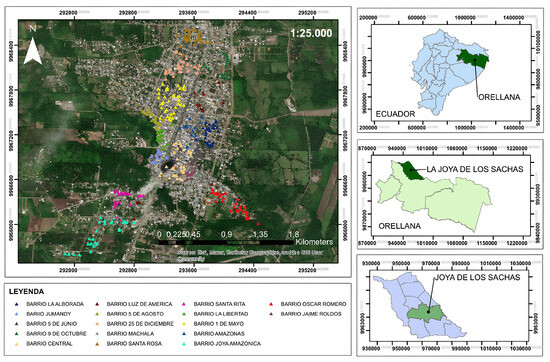
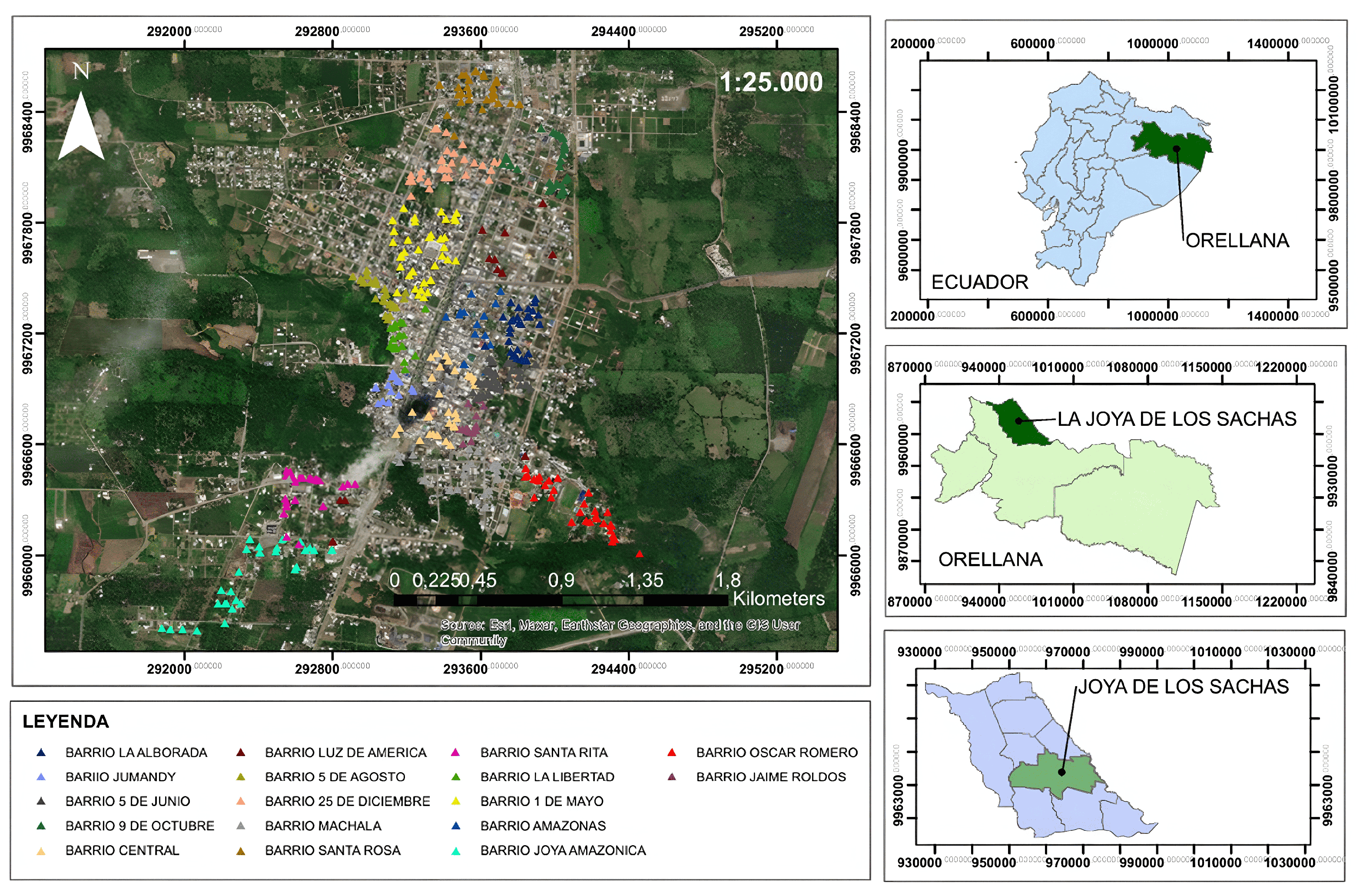
The analysis focuses on the urban core of La Joya de los Sachas (Orellana Province, Ecuador), which matches the MSW collection service area. The municipal system includes households, commercial establishments, markets, and street sweeping/municipal cleaning. Figure 1 shows the reference cartography (urban boundary and green areas) used to define the spatial scope of the characterization campaign. The observed period corresponds to a 69-day characterization campaign (69 effective days), detailed in the data collection subsection. For modeling, we use only generator types with a stable daily denominator (households, commercial establishments, and markets) to construct comparable per-denominator rates; street sweeping and municipal cleaning are excluded because they lack a reliable denominator and show high operational variability (Section 2.2).

Figure 1. Delimitation of the urban core of La Joya de los Sachas. Generated using ArcGIS Desktop 10.8. Source: municipal cartography [20] and Esri basemap data.

2.2. Data Collection and Sampling Design

2.2.1. Acquisition and Reference

Data come from a Municipal Solid Waste Characterization Study conducted in the urban core. The protocol followed the MINAM guidelines [21]. The goal was to obtain primary measurements with consistent recording and operational traceability. The adopted guideline [21] defines short, intensive characterization campaigns as operationally valid to estimate MSW generation in cities with heterogeneous sources, which supports the 69-day field window used in this study.

2.2.2. Coverage and Unit of Observation

Data collection followed a source–day panel design. Each record corresponds to one generator source measured on one calendar day. In this study, source refers to the generator category (households, commercial establishments, Municipal market, and San Francisco market), yielding four records per day. Fieldwork covered 8 May 2024 to 15 July 2024. After applying the measurement schedule and quality checks, the analysis uses 69 effective days. All measurements were checked for chronological consistency.

2.2.3. Scope by Generator Type

We included households, commercial establishments, and markets. These generators provide a stable daily denominator (persons per household or number of premises). This allows the construction of comparable rates over time. We excluded street sweeping and municipal cleaning. These services lack a reliable denominator (e.g., users served, swept area, roadway length, or labor-hours per day) and operate with high day-to-day variability. Under these conditions, rate normalization is not reliable. Including them would mix raw kg/day with normalized rates and would bias comparisons. Records with null or invalid denominators were removed.

Households, commercial establishments, and markets account for 5187.20 out of 5305.61 tonnes/year of MSW in the urban area (97.8%). Street sweeping and cleaning contribute 2.2%. The models therefore represent the dominant urban flows and the main recoverable fractions.

2.2.4. Sampling Strategy

Selection was adaptive by generator type, in accordance with the adopted methodological protocol (MINAM guidelines, 2018) [21]. Spatial sectorization was applied when operationally feasible to ensure coverage and logistics. Table 2 summarizes the parameters defined by the methodology: universe, recommended sample, effective participation, and the operating scheme by generator (commercial establishments, households, and markets), including measurement windows, operational scheduling, and the weighing method (kg using calibrated scales).

Table 2. Size and operation by generator type.

Aspect	Commercial Establishments	Households	Markets
Universe	1162 units (GADMLJS)	7550 dwellings (INEC)	2 markets (Municipal and San Francisco)
Recommended sample (EC-RSM)	110 observations	95 + 20% contingency = 114	Total coverage (both markets)
Effective participation	89 establishments	114 dwellings	2 markets
Measurement window	5 consecutive days per site	8 days per dwelling	7 days
Operational schedule	Daily pickup at 15:00; bag replacement	Daily pickup and bag replacement	Daily activity at 16:30; fixed collection points
Weighing	Daily weighing (kg) with calibrated scales	Daily weighing (kg) with calibrated scales	Daily weighing (kg) with calibrated scales

The characterization was designed to guarantee traceability and comparability across sources. The universes were established using official data: the Decentralized Autonomous Municipal Government of La Joya de los Sachas (GADMLJS) reported 1162 commercial establishments and 2 markets [20]; the National Institute of Statistics and Census (INEC) recorded 7550 households in the urban core [22]. Fieldwork followed the criteria of the EC-RSM [21]. In commercial establishments, for universes greater than 1000, the EC-RSM recommends a reference sample of 110; effective participation was 89 premises, with proportional allocation by sector. Five consecutive days were measured per premise, with waste removal at 15:00 and the provision/replacement of bags; the daily average of effective premises was 76. In households, 114 were selected with a 20% contingency. The measurement window was eight days per household; the first day was discarded to avoid carryover, and daily bag removal and replacement were maintained. In markets, due to their condition as major generators, a full census of the two establishments was applied, with fixed accumulation points and a seven-day schedule at 16:30. In all cases, weighing was performed daily, in kilograms, with calibrated scales and standardized recording. This uniform operational scheme ensures methodological coherence and enables valid comparisons across sources and fractions for subsequent modeling.

Field measurements are subject to unavoidable uncertainty. Although calibrated scales were used, effective precision depends on scale resolution, calibration drift, and field handling. Additional variability may arise from human recording errors (e.g., transcription mistakes) and participation or coverage constraints by generator type, which can introduce sampling bias. Uncertainty in the operational denominators (persons per household or number of premises) also propagates to the constructed rates and, after back-transformation, to kilogram-level predictions. These factors should be considered when interpreting performance estimates under a short observational horizon.

2.2.5. Fraction Classification

Segregation was performed into mutually exclusive operational categories: cardboard, paper, PET plastic (bottles), HDPE plastic (bags), colored glass, clear glass, metals (cans), Tetra Pak, food scraps, pruning and garden waste, wood and straw, sanitary, and other. Each category was defined by predominant material and typical use. The sanitary category groups hygienic–sanitary wastes requiring special handling; and the other aggregates non-recyclable or heterogeneous materials not classifiable in the previous categories. All fractions were weighed separately [21].

2.3. Dataset Construction and Feature Engineering

2.3.1. Structure and Consolidation for Modeling

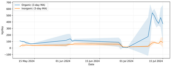
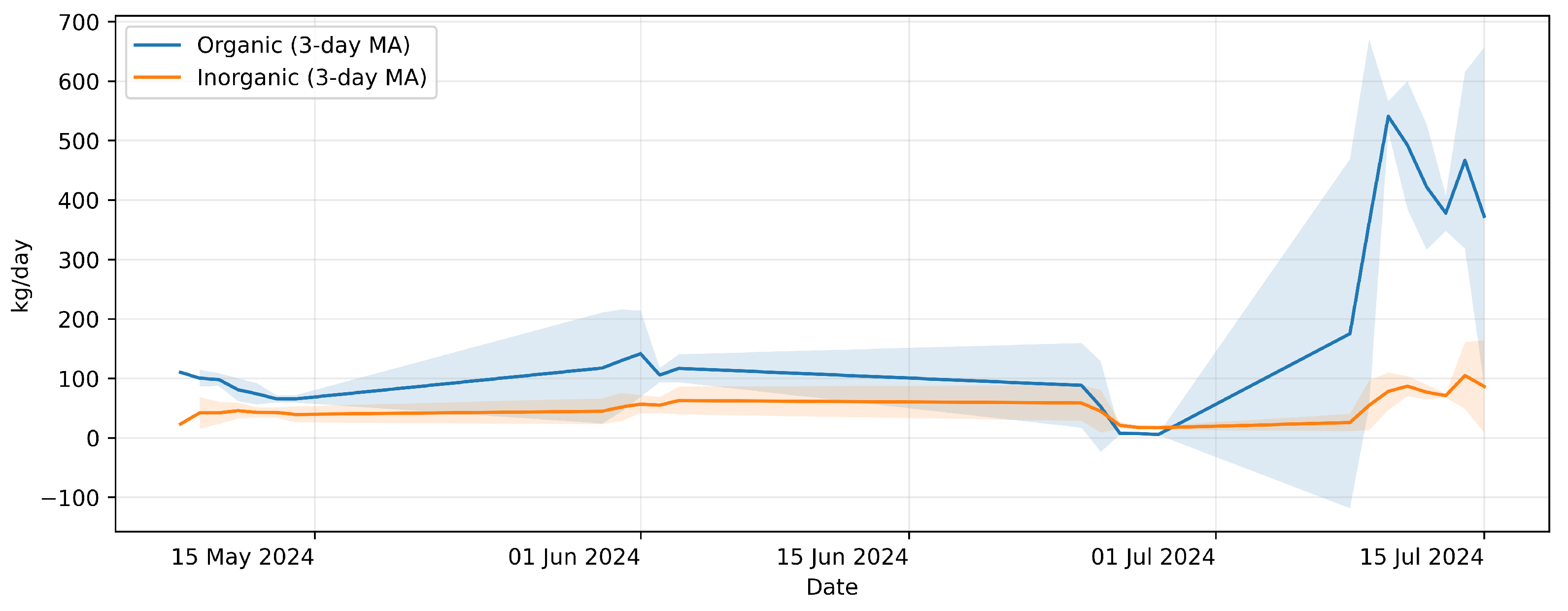
All measured categories were aggregated into two fractions: organic (kg) and inorganic (kg). Figure 2 shows their daily city-level evolution (3-day moving average) as a descriptive reference.

Figure 2. Daily generation of organic and inorganic waste (3-day moving average, kg/day).

2.3.2. Analytical Dataset and Fields

The raw dataset is a source–day panel. Each row is one generator source measured on one calendar day. Fields include:

• Fecha: day of measurement (ISO format, e.g., YYYY-MM-DD).
• Día: calendrical descriptor (e.g., day of the week/ISO week).
• Fuente de generación: standardized category (household, commercial establishment, market).
• Locales/viviendas: count of operational units per observation.
• N_Personas: number of persons per household.
• Organic (kg) and Inorganic (kg): daily masses weighed by fraction.

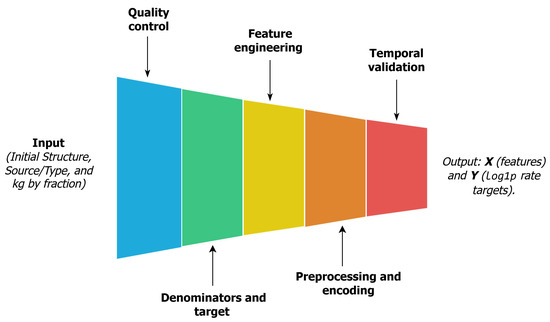
2.3.3. Quality Control

We cast dates to a temporal type and sorted records chronologically. We standardized generator labels, validated numeric fields, enforced non-negativity, and removed records with missing or invalid denominators. After cleaning, the analytical dataset contains $N=276$ source–day records spanning 8 May 2024 to 15 July 2024.

2.3.4. Denominators and Targets

A denominator was defined per observation: number of persons for households and number of premises for commercial establishments and markets (denominator > 0 required). We converted masses to rates (kg/person or kg/premise) and applied $log1p(·)$ to reduce heteroscedasticity. The targets are $y_{\mathrm{org}}$ and $y_{\mathrm{inorg}}$, both in $log1p\left(\mathrm{rate}\right)$ space.

2.3.5. Temporal Feature Engineering

We created short-horizon temporal predictors. Day-of-week and month were encoded with sine/cosine transforms. We added binary indicators for weekend, end-of-month, and fortnight, plus ISO-week components. We modeled source-specific memory with lag-1 and lag-7 rates, plus 7-day shifted moving averages, and their corresponding standard deviations. Denominator history was captured with lag-1 and a 7-day moving average. All lags and windows were computed within each source and shifted to avoid leakage.

2.3.6. Preprocessing and Encoding

All models were trained through a reproducible pipeline. Numerical features used median imputation and, when required, standardization. Categorical features used mode imputation and one-hot encoding with unknown categories enabled. In each split, preprocessing was fitted only on the training window.

2.3.7. Temporal Validation

We used a daily expanding-window scheme. In split s, the model is trained on all observations up to day t and tested on day t + 1. This preserves temporal causality and prevents the use of future information.

2.3.8. Workflow Output

The workflow yields X (feature matrix) and Y (two targets in $log1p$ of rates). For interpretation in kilograms, predictions are inverted as in Equation (1), where D is the observation denominator:

$$\begin{array}{c}\mathrm{kg}=expm1\left(\widehat{y}\right)\times D\hfill \end{array}$$

(1)

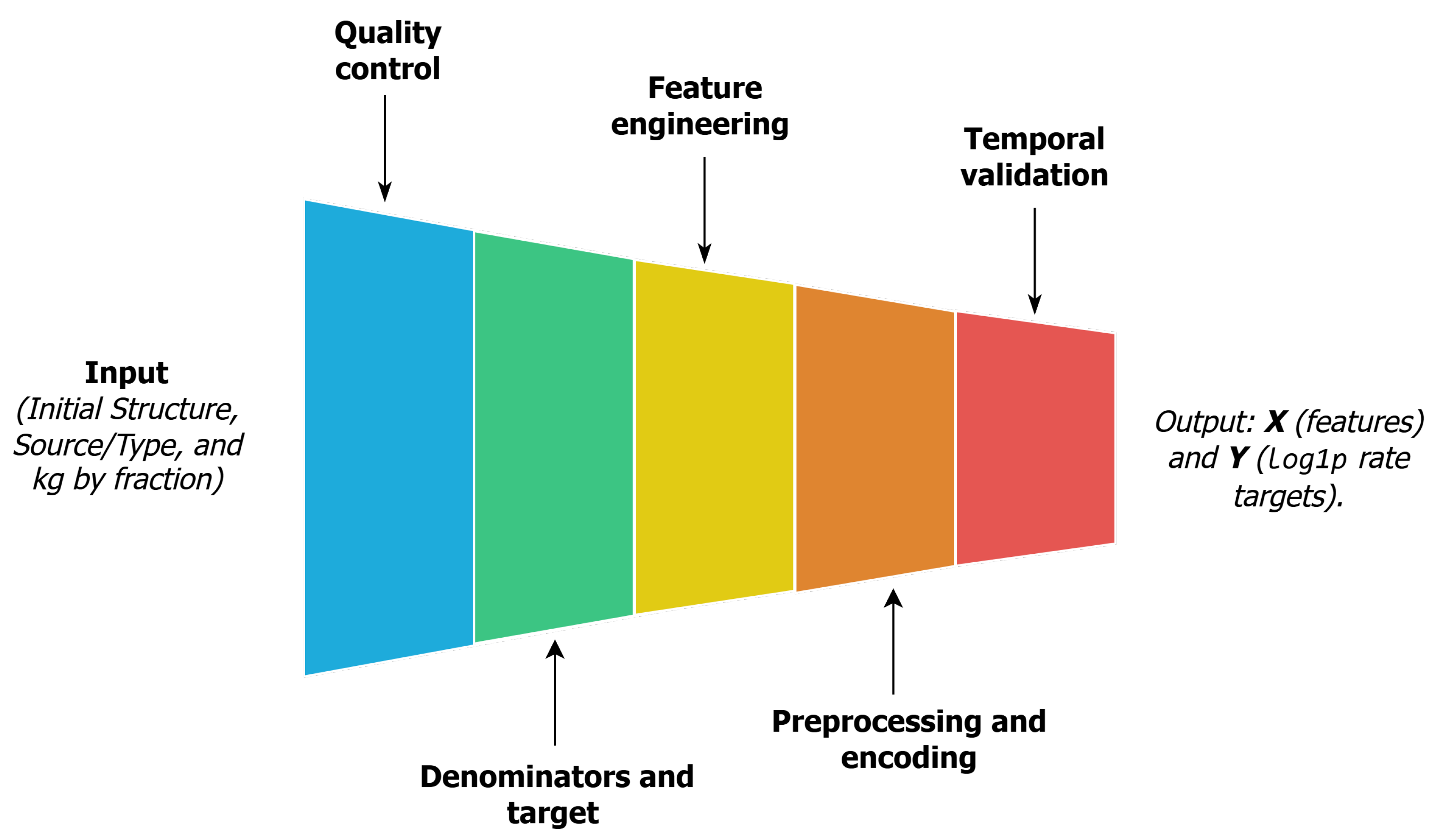
Figure 3 shows a diagram of the data preparation and temporal validation pipeline, integrating all the phases described.

Figure 3. Diagram of the data preparation pipeline.

2.4. Modeling

We framed the task as multi-output regression with two continuous targets per observation: $y_{\mathrm{org}}$ and $y_{\mathrm{inorg}}$. Each target is defined as $log1p\left(\mathrm{rate}\right)$ (kg per denominator). This transform reduces heteroscedasticity and attenuates extreme values. Inputs include calendar descriptors, source-specific lags and moving averages, denominator history, and categorical encodings.

We adopted a multi-output formulation because organic and inorganic fractions are measured jointly each day and share the same operational and temporal predictors, which allows a consistent protocol and comparable evaluation across fractions.

We evaluated fourteen tabular regression models: Linear Regression, Ridge, Lasso, ElasticNet, SVR, KNN, MLPRegressor, Decision Tree, Random Forest, Extra Trees, Gradient Boosting, AdaBoost, XGBoost, and LightGBM. Decision Tree, Random Forest, and Extra Trees were fitted with native multi-output support. The remaining estimators were wrapped with MultiOutputRegressor. In those cases, the two outputs are learned independently using separate regressors with the same feature set. Therefore, cross-output correlation between organic and inorganic fractions is not explicitly modeled. Modeling such correlation (e.g., multi-task or structured-output approaches) is left for future work.

Each model was implemented as a scikit-learn Pipeline with a ColumnTransformer (Table 3). Numerical features used median imputation and, for scale-sensitive models (linear models, SVR, KNN, MLP), standardization to zero mean and unit variance. Categorical features used mode imputation and one-hot encoding with support for unseen categories. Tree-based methods were trained without scaling. In every split, preprocessing was fitted only on the training window to prevent leakage.

Table 3. Summary of the regression models and preprocessing strategy.

Family	Model	Abbreviation	Scaling of Inputs	Multi-Output Handling
Linear models	Linear Regression, Ridge, Lasso, ElasticNet	LR, Ridge, Lasso, ENet	Standardization	MultiOutputRegressor (independent outputs)
Support Vector Machines	Support Vector Regressor	SVR	Standardization	MultiOutputRegressor (independent outputs)
Neighbors	k-Nearest Neighbors Regressor	KNN	Standardization	MultiOutputRegressor (independent outputs)
Shallow neural networks	Multi-Layer Perceptron Regressor	MLP	Standardization	MultiOutputRegressor (independent outputs)
Tree-based methods	Decision Tree Regressor	DT	No scaling	Native multi-output
Tree-based ensembles	Random Forest, Extra Trees, Gradient Boosting, AdaBoost	RF, ET, GB, AB	No scaling	RF/ET: native multi-output; GB/AB: MultiOutputRegressor (independent outputs)
Gradient boosting trees	XGBoost Regressor, LightGBM Regressor	XGB, LGBM	No scaling	MultiOutputRegressor (independent outputs)

Hyperparameter tuning used GridSearchCV with model-specific search spaces (Table 4). We tuned $\alpha$ (and $l_1$-ratio for ElasticNet), $(C,ϵ)$ for SVR with an RBF kernel, k for KNN, and depth/leaf constraints for tree ensembles. For boosting methods, we tuned learning rate and tree complexity. For XGBoost and LightGBM, we included depth/leaf parameters and subsampling to constrain model capacity. The MLPRegressor used $L_2$ regularization with internal early stopping.

Table 4. Hyperparameter search space for the main model families.

Model	Hyperparameter	Values Explored
Ridge	$\alpha$ (L2 penalty)	$\alpha \in \{{10}^{-4},{10}^{-3},{10}^{-2},{10}^{-1},1.0\}$
Lasso	$\alpha$ (L1 penalty)	$\alpha \in \{{10}^{-4},5\times {10}^{-4},{10}^{-3},5\times {10}^{-3},{10}^{-2}\}$; max_iter = 10,000
ElasticNet	$\alpha$, $l_1$-ratio	$\alpha \in \{5\times {10}^{-4},{10}^{-3},5\times {10}^{-3},{10}^{-2}\}$; $l_1$-ratio $\in \{0.1,0.5,0.9\}$; max_iter = 10,000
SVR	C, $ϵ$, kernel	$C\in \{0.5,1,2\}$; $ϵ\in \{0.01,0.05,0.1\}$; kernel = RBF
KNN	Number of neighbors	$k\in \{3,5,7\}$
Random Forest/Extra Trees	$n_{\mathrm{estimators}}$, max depth, min samples per leaf	$n_{\mathrm{estimators}}=300$; max_depth $\in \{6,8,10\}$; min_samples_leaf $\in \{1,3,5\}$
Gradient Boosting	$n_{\mathrm{estimators}}$, learning rate, max depth	$n_{\mathrm{estimators}}=300$; learning_rate $\in \{0.05,0.1\}$; max_depth $\in \{2,3\}$
AdaBoost	$n_{\mathrm{estimators}}$, learning rate	$n_{\mathrm{estimators}}=300$; learning_rate $\in \{0.05,0.1\}$
XGBoost	$n_{\mathrm{estimators}}$, max depth, learning rate, subsampling	$n_{\mathrm{estimators}}=300$; max_depth $\in \{3,4\}$; learning_rate $\in \{0.05,0.1\}$; subsample $\in \{0.8,1.0\}$; colsample_bytree $\in \{0.8,1.0\}$
LightGBM	num leaves, learning rate, $n_{\mathrm{estimators}}$	num_leaves $\in \{15,31\}$; learning_rate $\in \{0.05,0.1\}$; $n_{\mathrm{estimators}}=300$

2.5. Temporal Validation and Evaluation Metrics

We used daily expanding-window backtesting to preserve temporal causality (Table 5). In each split s, the model is trained on all observations up to day $t_s-1$ and evaluated on day $t_s$ (one-step-ahead). Each test block corresponds to one calendar day and includes all source-level records available on that day (four observations, one per generator category). All preprocessing steps are fitted only on the training window of each split to prevent information leakage.

Table 5. Temporal backtesting protocol, baselines, and evaluation criterion.

Element	Description
Cross-validation scheme	Daily expanding-window backtesting (one-step-ahead). For each split s, the training set contains all observations up to day $t_s-1$ and the test set corresponds to day $t_s$. Each test block is one calendar day and includes all source-level records available on that day.
Sample sizes	We obtained $S=13$ splits. Training blocks contain 224–272 observations (56–68 days). Each test block contains 4 observations from a single day (one per generator category). Total out-of-sample observations: 52.
Baselines	(i) Lag-7 persistence in rate space per source and fraction (fallback to lag-1 and to the historical median when required). (ii) ARIMA benchmark fitted only on the training window of each split and used to produce a one-step-ahead forecast for day $t_s$.
Model selection criterion	Custom scorer for GridSearchCV: mean $\mathrm{MAE}$ in rate space, computed after inverting $\log 1p(·)$ with $\mathrm{expm}1(·)$, and averaged over the two targets ($y_{\mathrm{org}}$ and $y_{\mathrm{inorg}}$). Final comparisons are reported per fraction (organic and inorganic).
Evaluation metrics	$\mathrm{MAE}$, $\mathrm{RMSE}$, $R^2$, and Nash–Sutcliffe efficiency ($\mathrm{NSE}$) for each fraction, plus pseudo-$R^2$ relative to the lag-7 persistence baseline.
Uncertainty quantification	Day-cluster bootstrap over out-of-sample predictions, resampling test days to preserve within-day dependence. We report 95% confidence intervals for $\mathrm{MAE}$ and $R^2$ for each fraction.
Implementation	GridSearchCV with cv = splits. All preprocessing steps (imputation, scaling, encoding) are fitted only on the training partition of each split to avoid information leakage.

In our setup we obtained $S=13$ splits. Training blocks contain 224–272 observations (56–68 days), and each test block contains 4 observations from a single day. This yields 52 out-of-sample observations in total.

Hyperparameter tuning used GridSearchCV with cv = splits and a custom scorer based on the mean $\mathrm{MAE}$ in rate space, averaged over the organic and inorganic targets after inverting $\log 1p(·)$ with $\mathrm{expm}1(·)$. We report $\mathrm{MAE}$, $\mathrm{RMSE}$, $R^2$, and Nash–Sutcliffe efficiency ($\mathrm{NSE}$) for each fraction. We also report pseudo-$R^2$ relative to the lag-7 persistence baseline.

To account for the short time horizon and within-day dependence, we quantify uncertainty using a day-cluster bootstrap over out-of-sample predictions and report 95% confidence intervals for $\mathrm{MAE}$ and $R^2$ for each fraction. As summarized in Table 4, baselines include lag-7 persistence (with fallbacks) and an ARIMA benchmark trained only on each split’s training window.

2.6. Explainability Analysis

2.6.1. SHAP

We interpret the fitted model(s) using SHAP [23]. Explanations are computed on the same scikit-learn pipeline used for forecasting. Because most estimators are trained with MultiOutputRegressor, the organic and inorganic outputs are explained separately using one explainer per output. SHAP values are computed in the transformed target space, where the targets are defined as $log1p\left(\mathrm{rate}\right)$ (kg per denominator), consistent with the learning objective.

SHAP values are computed on the preprocessed feature matrix obtained by applying the fitted ColumnTransformer to the full feature table X. Global importance is summarized with bee swarm plots, reporting the top 15 predictors for each fraction. All analyses were implemented in Python 3.12.12 using the shap library and matplotlib.

2.6.2. LIME

We complement SHAP with LIME [24] to provide local explanations for individual predictions. LIME is applied in regression mode on the same fitted pipeline, operating in the preprocessed feature space. We select representative instances from the recent period: (i) an organic peak day with relatively high absolute error, (ii) a typical day with low error, and (iii) a low-generation day. For each instance, LIME fits a sparse local linear surrogate using 5000 perturbed samples and reports the 10 most influential predictors.

Together, SHAP and LIME verify that the model primarily relies on operationally meaningful signals (source category, short-term autoregressive terms such as lags and moving averages, denominator-related predictors, and calendar indicators) rather than on arbitrary patterns.

3. Results and Discussion

3.1. Evaluation of the Performance of ML Models

We evaluated fourteen regression algorithms to forecast daily MSW generation by fraction (organic and inorganic). Predictors combine calendar descriptors, short-horizon memory terms computed from the rate series (lags and 7-day rolling statistics), and an operational denominator by generator category (persons or premises). Performance was assessed with daily expanding-window backtesting to preserve temporal causality, training on past observations and testing on the next day. Final metrics are computed over pooled OOS predictions from 13 one-day test blocks (52 observations).

To quantify statistical uncertainty under the short time horizon and within-day dependence, we report 95% confidence intervals using a day-cluster bootstrap over pooled out-of-sample predictions (resampling test days). Intervals are computed in rate space. These uncertainty estimates are summarized in Table 6.

Table 6. Day-cluster bootstrap uncertainty (95% CI) for the selected models computed over pooled out-of-sample predictions in rate space.

Metric	Organic (AdaBoost)	Inorganic (Random Forest)
$R^2$	$0.985[0.982,0.988]$	$0.963[0.953,0.973]$
$\mathrm{MAE}$	$0.062[0.053,0.071]$	$0.040[0.034,0.046]$

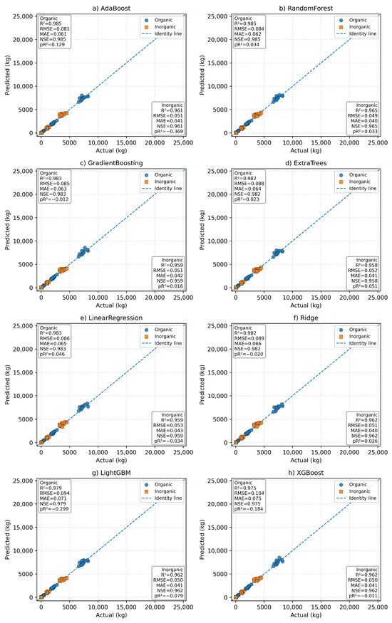
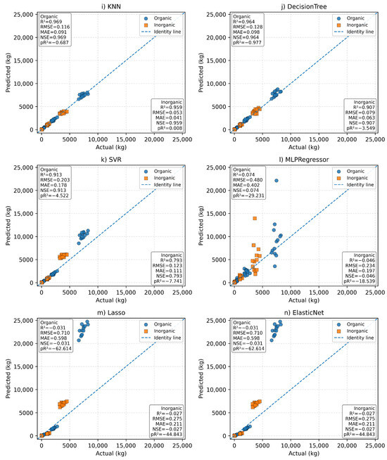
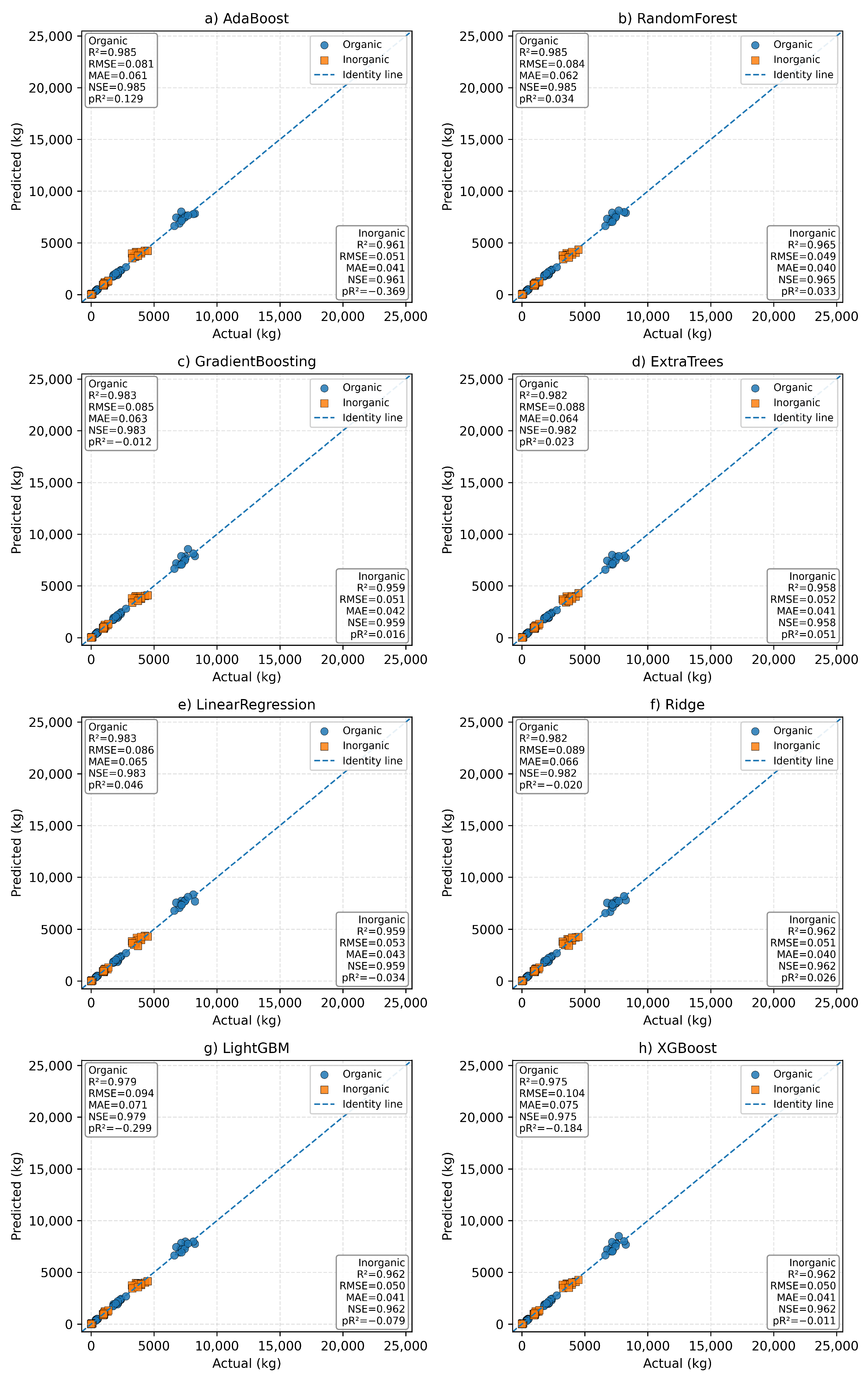
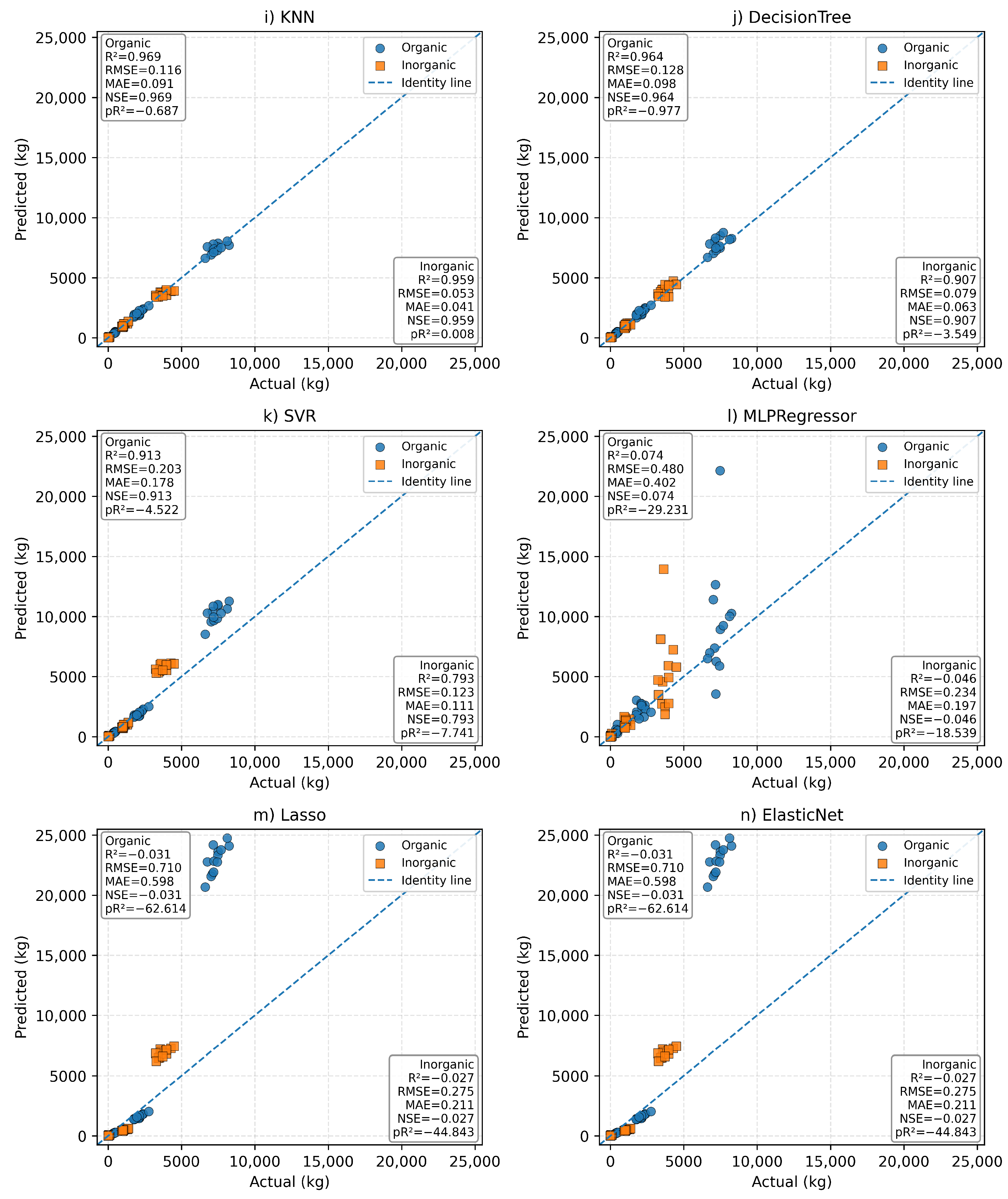
Figure 4 shows observed versus predicted values in kilograms after inverting the target transformation ($\mathrm{kg}=expm1\left(\widehat{y}\right)\times D$). Most models concentrate near the identity line, with tighter dispersion for the inorganic fraction. The plots also reveal systematic degradation for SVR, MLPRegressor, and the penalized linear models, which exhibit larger deviations and, in some cases, clear bias away from the identity line. This visual pattern is consistent with the test metrics in Table 7 and Table 8, which are reported in rate space.

Figure 4. Observed vs. predicted (kg) in the test set for the organic and inorganic fractions: (a) AdaBoost Regressor; (b) Linear Regression; (c) Random Forest Regressor; (d) Ridge; (e) Extra Trees Regressor; (f) XGBoost Regressor; (g) Gradient Boosting Regressor; (h) LightGBM Regressor; (i) Decision Tree Regressor; (j) k-Nearest Neighbors Regressor (KNN); (k) Support Vector Regressor (SVR); (l) Multi-Layer Perceptron Regressor (MLP); (m) Lasso; (n) Elastic Net.

Table 7. Model performance (organic fraction, rate space): train/test metrics ($\mathrm{RMSE}$, $R^2$, $\mathrm{NSE}$, $\mathrm{MAE}$) and pseudo-$R^2$ vs. lag-7 persistence.

Model	Testing Data Set Performance				Training Data Set Performance				Baseline
	$\mathbf{RMSE}$	${\mathit{R}}^{\mathbf{2}}$	$\mathbf{NSE}$	$\mathbf{MAE}$	$\mathbf{RMSE}$	${\mathit{R}}^{\mathbf{2}}$	$\mathbf{NSE}$	$\mathbf{MAE}$	Pseudo- ${\mathit{R}}^{\mathbf{2}}$ (vs. lag-7)
AdaBoost	0.081	0.985	0.985	0.061	0.084	0.986	0.986	0.061	0.129
RandomForest	0.084	0.985	0.985	0.062	0.047	0.996	0.996	0.033	0.034
GradientBoosting	0.085	0.983	0.983	0.063	0.038	0.997	0.997	0.028	−0.012
ExtraTrees	0.088	0.982	0.982	0.064	0.040	0.997	0.997	0.026	0.023
LinearRegression	0.086	0.983	0.983	0.065	0.083	0.986	0.986	0.060	0.046
Ridge	0.089	0.982	0.982	0.066	0.093	0.983	0.983	0.067	−0.020
LightGBM	0.094	0.979	0.979	0.071	0.040	0.997	0.997	0.029	−0.299
XGBoost	0.104	0.975	0.975	0.075	0.028	0.998	0.998	0.021	−0.184
KNN	0.116	0.969	0.969	0.091	0.156	0.951	0.951	0.091	−0.687
DecisionTree	0.128	0.964	0.964	0.098	0.000	1.000	1.000	0.000	−0.977
SVR	0.203	0.913	0.913	0.178	0.171	0.942	0.942	0.141	−4.522
MLPRegressor	0.480	0.074	0.074	0.402	0.300	0.808	0.808	0.225	−29.231
Lasso	0.710	−0.031	−0.031	0.598	0.717	−0.025	−0.025	0.603	−62.614
ElasticNet	0.710	−0.031	−0.031	0.598	0.717	−0.025	−0.025	0.603	−62.614

Table 8. Model performance (inorganic fraction, rate space): train/test metrics ($\mathrm{RMSE}$, $R^2$, $\mathrm{NSE}$, $\mathrm{MAE}$) and pseudo-$R^2$ vs. lag-7 persistence.

Model	Testing Data Set Performance				Training Data Set Performance				Baseline
	$\mathbf{RMSE}$	${\mathit{R}}^{\mathbf{2}}$	$\mathbf{NSE}$	$\mathbf{MAE}$	$\mathbf{RMSE}$	${\mathit{R}}^{\mathbf{2}}$	$\mathbf{NSE}$	$\mathbf{MAE}$	Pseudo- ${\mathit{R}}^{\mathbf{2}}$ (vs. lag-7)
RandomForest	0.049	0.965	0.965	0.040	0.026	0.990	0.990	0.019	0.033
Ridge	0.051	0.962	0.962	0.040	0.049	0.963	0.963	0.036	0.026
AdaBoost	0.051	0.961	0.961	0.041	0.036	0.980	0.980	0.030	−0.369
LightGBM	0.050	0.962	0.962	0.041	0.022	0.993	0.993	0.016	−0.079
XGBoost	0.050	0.962	0.962	0.041	0.015	0.997	0.997	0.011	−0.011
ExtraTrees	0.052	0.958	0.958	0.041	0.020	0.994	0.994	0.015	0.051
KNN	0.053	0.959	0.959	0.041	0.061	0.943	0.943	0.038	0.008
GradientBoosting	0.051	0.959	0.959	0.042	0.019	0.995	0.995	0.015	0.016
LinearRegression	0.053	0.959	0.959	0.043	0.047	0.967	0.967	0.035	−0.034
DecisionTree	0.079	0.907	0.907	0.063	0.000	1.000	1.000	0.000	−3.549
SVR	0.123	0.793	0.793	0.111	0.102	0.839	0.839	0.091	−7.741
MLPRegressor	0.234	−0.046	−0.046	0.197	0.149	0.582	0.582	0.113	−18.539
Lasso	0.275	−0.027	−0.027	0.211	0.256	−0.006	−0.006	0.205	−44.843
ElasticNet	0.275	−0.027	−0.027	0.211	0.256	−0.006	−0.006	0.205	−44.843

Across candidates, the best generalization is obtained with tree-based ensembles and strong linear benchmarks. For the organic fraction (Table 7), AdaBoost achieves the lowest test error ($\mathrm{RMSE}$ $=0.081$, $\mathrm{MAE}$ $=0.061$, $R^2$ $=0.985$), followed closely by Random Forest ($\mathrm{RMSE}$ $=0.084$, $\mathrm{MAE}$ $=0.062$, $R^2$ $=0.985$) and the remaining top ensembles (Gradient Boosting, Extra Trees) and Linear Regression, all with $R^2$ $\approx 0.98$ and $\mathrm{RMSE}$ below $0.09$. For the inorganic fraction (Table 8), Random Forest provides the best overall performance ($\mathrm{RMSE}$ $=0.049$, $\mathrm{MAE}$ $=0.040$, $R^2$ $=0.965$), with Ridge, Extra Trees, and Gradient Boosting showing very similar accuracy. These results indicate that, within this dataset, short-horizon autoregressive structure and denominator-driven scaling are highly informative, and flexible ensembles can exploit them reliably under temporal evaluation.

To address concerns about whether high $R^2$ values simply reflect a strong autoregressive baseline, we also report pseudo-$R^2$ relative to a lag-7 persistence benchmark. In the organic fraction, several models improve over lag-7 persistence (e.g., AdaBoost pseudo-$R^2$ $=0.129$; Linear Regression $0.046$; Random Forest $0.034$), while others are close to parity or slightly worse (e.g., Gradient Boosting $-0.012$). In the inorganic fraction, improvements over lag-7 persistence are smaller but still present for key ensembles (e.g., Extra Trees $0.051$; Random Forest $0.033$). This comparison supports that the best-performing models provide predictive skill beyond naive weekly repetition, though gains are fraction-dependent and modest in some cases.

In addition to lag-7 persistence, ARIMA provides a complementary autoregressive benchmark in rate space, achieving $\mathrm{MAE}$ $=0.0890$, $\mathrm{RMSE}$ $=0.1124$, and $R^2$ $=0.9691$ for the organic fraction and $\mathrm{MAE}$ $=0.0428$, $\mathrm{RMSE}$ $=0.0516$, and $R^2$ $=0.9567$ for the inorganic fraction; these values remain below the best ML models, supporting the added value of the proposed pipelines.

Methods that are sensitive to scaling and local neighborhoods (KNN, SVR, and MLPRegressor) show a clear loss of accuracy under backtesting, and the penalized linear models (Lasso and ElasticNet) fail to recover stable coefficients in this short, heterogeneous setting, yielding near-zero or negative $R^2$ and strongly negative pseudo-$R^2$.

The results support tree-based ensembles as the most reliable family under temporal backtesting, with AdaBoost leading in the organic fraction ($\mathrm{RMSE}$ $=0.081$, $R^2$$=0.985$) and Random Forest leading in the inorganic fraction ($\mathrm{RMSE}$ $=0.049$, $R^2$$=0.965$). This behavior is consistent with municipal MSW settings where generator heterogeneity and short-horizon dynamics create nonlinear effects that are well captured by ensemble models [25,26]. At the same time, the organic fraction shows several near-ties (e.g., Linear Regression and the top ensembles), indicating that the engineered autoregressive and denominator features explain most of the signal in that series. Finally, using multiple metrics ($\mathrm{MAE}$, $\mathrm{RMSE}$, $R^2$, $\mathrm{NSE}$) together with baseline-relative skill (pseudo-$R^2$ vs. lag-7) enables a more robust comparison and avoids over-reliance on a single goodness-of-fit statistic under a limited time horizon [27,28].

3.2. Temporal Representativeness and Generalization Limits

This study relies on a short observational window. With a limited number of unique days, the evaluation is exposed to higher uncertainty and a higher risk of overfitting, especially given the number of candidate models, the hyperparameter tuning procedure, and the engineered feature set (calendar encodings, lags, and moving averages). In this setting, high goodness-of-fit values can be inflated by strong short-term persistence and by the limited diversity of temporal conditions covered.

We mitigate these risks with strict temporal backtesting. We use daily expanding-window one-step-ahead evaluation and fit all preprocessing steps only on the training block of each split to prevent leakage. We also benchmark against strong autoregressive baselines, including lag-7 persistence, and we quantify uncertainty with day-cluster bootstrap confidence intervals for $\mathrm{MAE}$ and $R^2$ based on pooled out-of-sample predictions. These steps provide a more conservative estimate of performance than a single hold-out split.

Despite these controls, the current window does not cover longer seasonal cycles or broader operational variation. Therefore, stability across seasons cannot be claimed. In addition, the analysis is limited to one municipality and a fixed operational context. Generalization to other cities requires external validation under different demographic, climatic, and service conditions, and periodic re-calibration when deployed.

3.3. Loss Curves and Error Diagnostics of the Selected Models

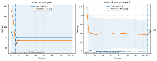
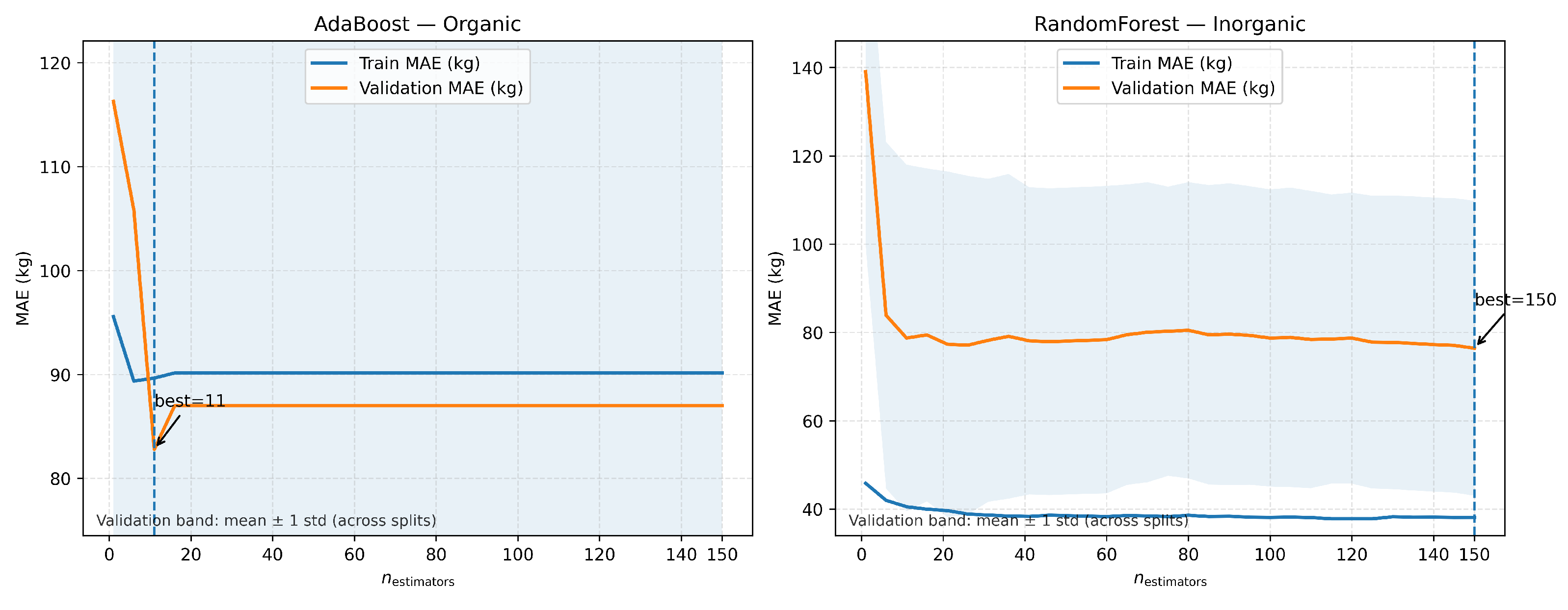
To complement the aggregate metrics in Table 7 and Table 8, we report diagnostic curves and point-wise error profiles for the selected models in each fraction. Figure 5 shows training and validation $\mathrm{MAE}$ curves in kilograms under the same temporal backtesting protocol used for model evaluation. For the organic fraction, AdaBoost reaches its lowest validation $\mathrm{MAE}$ early (around $n_{\mathrm{estimators}}\approx 11$) and then stabilizes, indicating that additional estimators do not improve generalization. For the inorganic fraction, Random Forest attains its best validation $\mathrm{MAE}$ within the evaluated grid at a larger ensemble size (around $n_{\mathrm{estimators}}\approx 150$), with stable training loss and a relatively flat validation profile after the initial decrease. These diagnostics support the model selection reported in Table 7 and Table 8 and highlight that the two fractions require different ensemble capacities.

Figure 5. Training and validation $\mathrm{MAE}$ curves (kg) under temporal backtesting for the selected models: AdaBoost (organic) and Random Forest (inorganic). The dashed line marks the minimum validation $\mathrm{MAE}$.

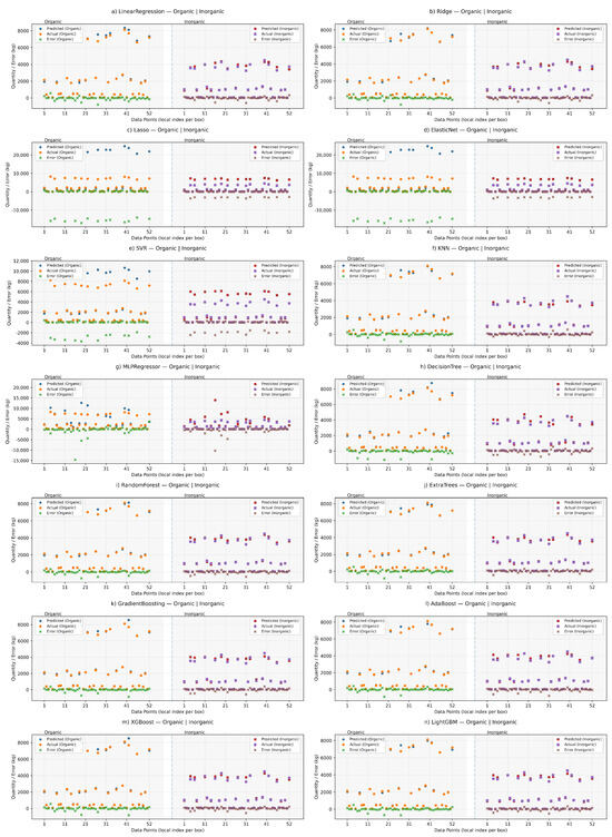
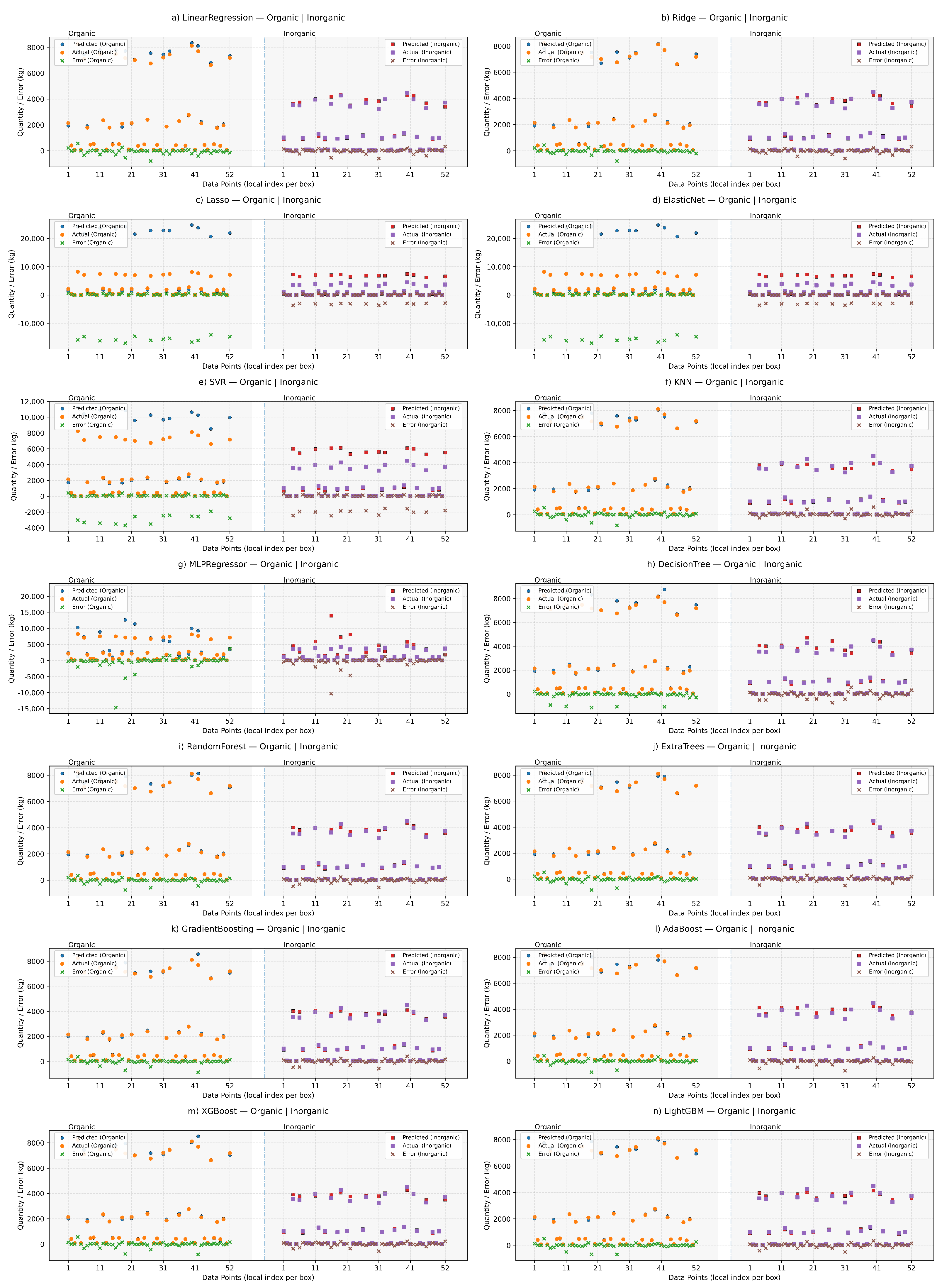
Figure 6 presents point-wise predictions and prediction errors in kilograms across the pooled out-of-sample evaluations. The inorganic fraction shows smaller dispersion and smaller error magnitudes across models, while the organic fraction exhibits larger deviations around high-generation days. This pattern is visible even for the strongest models and is consistent with the higher sensitivity of organic waste to unobserved external drivers and operational variability. In contrast, weak baselines for this dataset (Lasso, ElasticNet, and MLPRegressor) show large systematic errors, confirming their limited suitability under the temporal protocol.

Figure 6. Point-wise observed and predicted values with prediction errors (kg) in the test set for the organic and inorganic fractions across all models.

Overall, the diagnostic evidence confirms two stable behaviors: (i) inorganic waste is more predictable and yields smaller errors; and (ii) organic waste concentrates larger errors during peaks. These peak deviations suggest that incorporating exogenous variables (e.g., rainfall, holidays, local events, and operational disruptions) could further reduce organic errors, particularly during atypical days. Consistent with Table 7 and Table 8, the selected models remain AdaBoost for organic and Random Forest for inorganic, with other tree ensembles providing competitive performance within a narrow margin.

3.4. Feature Importance Analysis

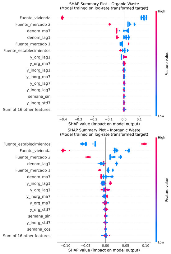
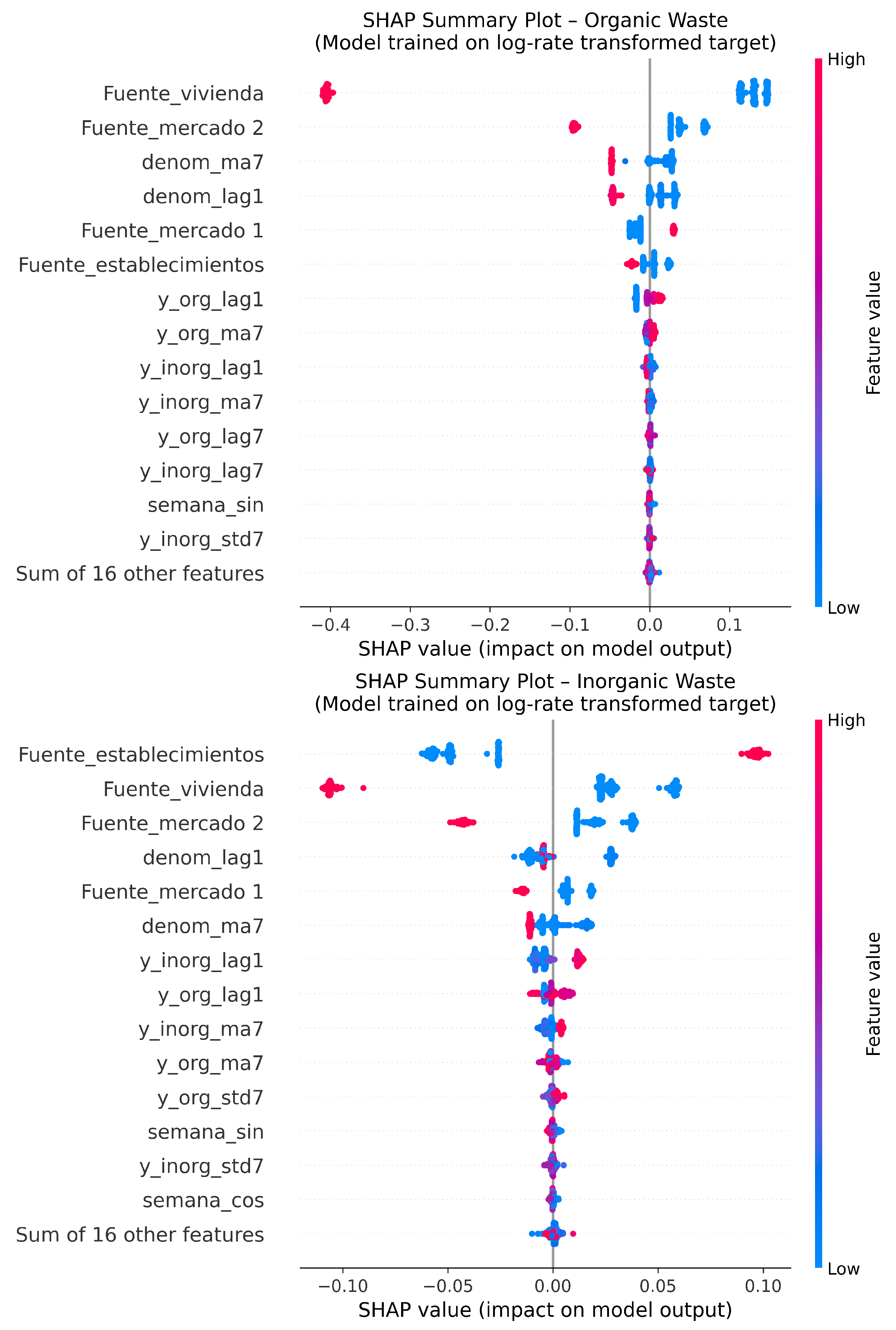
Figure 7 summarizes global feature importance using SHAP for the selected models in each fraction, computed in the log-rate target space. For the organic fraction (top panel), generator-category indicators dominate the explanation, led by Fuente_vivienda and the two market indicators (Fuente_mercado 1 and Fuente_mercado 2). Denominator history (denom_ma7, denom_lag1) also ranks among the most influential predictors, confirming that source scale (persons/premises) and its short-term variation shape the expected organic rate. Short-horizon memory terms from both fractions (y_org_lag1, y_org_ma7, y_inorg_lag1, y_inorg_ma7, y_org_lag7, y_inorg_lag7) appear next, indicating that organic predictions are largely driven by recent autoregressive structure and cross-fraction co-movement in the engineered lags.

Figure 7. SHAP summary plot (bee swarm) for the selected models in each fraction, computed on the log-rate target space: organic (top) and inorganic (bottom).

For the inorganic fraction (bottom panel), Fuente_establecimientos and Fuente_vivienda are the strongest drivers, followed by market indicators and denominator terms (denom_lag1, denom_ma7). Lagged inorganic and organic signals (y_inorg_lag1, y_inorg_ma7, y_org_lag1, y_org_ma7) remain consistently relevant, supporting that the model leverages short-term persistence and cross-fraction information even when the two outputs are learned independently. Weekly calendar terms (semana_sin and semana_cos) appear with smaller but non-negligible effects, suggesting a mild weekly seasonal component beyond the explicit lag features.

Local LIME explanations on representative test instances (including organic peak days and typical low-error days) are consistent with the SHAP ranking. The dominant contributions are associated with generator category, recent lags and rolling statistics of the rate series, and denominator-related variables, while calendar terms play a secondary role. Together, SHAP and LIME indicate that the models rely on operationally meaningful signals (source type, short-term persistence, and scale effects) rather than arbitrary correlations. From an operational standpoint, these results emphasize the value of maintaining consistent daily records by generator category and keeping denominators (persons/premises) up to date. The remaining organic peak errors further motivate incorporating exogenous drivers (e.g., rainfall, holidays, local events, or service disruptions) in future extensions.

3.5. Environmental and Operational Aspects of MSW Modeling

The MSW characterization for La Joya de los Sachas estimates a total municipal solid waste generation of 14.54 t/day, with 67.46% organic waste (9.81 t/day) and 15.52% recyclable materials (2.26 t/day). This composition supports circular strategies such as composting, material recovery, and landfill bio gas utilization [29].

Within this context, the forecasting errors of the selected models are small relative to the daily municipal flows. At city level, the mean absolute error is 246.62 kg/day for the organic fraction, 141.45 kg/day for the inorganic fraction, and 306.23 kg/day for total MSW (pooled out-of-sample predictions across temporal backtesting). These values represent approximately 2.51% of daily organic generation (246.62 kg over 9.81 t), 2.99% of daily inorganic generation (141.45 kg over ∼4.73 t), and 2.11% of total daily MSW (306.23 kg over 14.54 t). Assuming a typical compactor–truck capacity of 6000–8000 kg, the total absolute error corresponds to roughly 3.8–5.1% of one truck load per day, well below a full trip.

In addition, the selected models reduce error substantially relative to the lag-7 persistence baseline in operational units. Compared with the baseline, $\mathrm{MAE}$ decreases from 453.20 to 246.62 kg/day for organic waste, from 313.00 to 141.45 kg/day for inorganic waste, and from 612.71 to 306.23 kg/day for total MSW. This improvement indicates that the forecasting pipeline adds practical value beyond naive weekly repetition when predictions are interpreted at the city scale.

Operationally, this uncertainty level lies within typical safety margins used in fleet sizing and collection scheduling. The forecasts are therefore suitable to support day-ahead decisions on vehicle allocation, route planning, and frequency adjustments without compromising service reliability. Environmentally, aligning predictions with observed variability reduces systematic over/underestimation, helps avoid unnecessary trips, and improves planning of organic-rich streams for composting or bio gas recovery.

4. Conclusions

We compared fourteen ML algorithms for one-day-ahead forecasting of municipal solid waste in La Joya de los Sachas, disaggregated into organic and inorganic fractions, using a strict daily expanding-window backtesting protocol. The main conclusions are as follows:

• Best models (rate space): Performance is fraction-dependent. AdaBoost achieved the best test results for organic waste ($\mathrm{RMSE}$ $=0.081$, $\mathrm{MAE}$ $=0.061$, $R^2=0.985$). Random Forest achieved the best test results for inorganic waste ($\mathrm{RMSE}$ $=0.049$, $\mathrm{MAE}$ $=0.040$, $R^2=$ 0.965). SVR, KNN, MLPRegressor, Lasso, and ElasticNet degraded under temporal validation.
• Baseline comparison: The leading models provide skill beyond lag-7 persistence, with positive pseudo-$R^2$ for the top configurations in both fractions.
• Operational error (kg/day): At city level, mean absolute error is 246.62 kg/day (organic), 141.45 kg/day (inorganic), and 306.23 kg/day (total). This corresponds to 2.51% of daily organic generation, 2.99% of daily inorganic generation, and 2.11% of total MSW. Total $\mathrm{MAE}$ decreases from 612.71 to 306.23 kg/day relative to lag-7 persistence. The total error is 3.8–5.1% of a typical compactor–truck load (6000–8000 kg).
• What drives predictions: SHAP and LIME show that generator-category indicators, denominator history, and short-horizon lag/rolling features dominate importance. Calendar terms have a smaller effect.
• Contribution: We provide a reproducible protocol for short-horizon fraction-level MSW forecasting in data-scarce settings, with strict temporal validation, explicit baselines, and operational interpretation in kg/day.
• Limitations: The observational window is short and does not cover longer seasonal cycles. The study is limited to one municipality. Generalization requires external validation in other cities and longer time spans.

Future work will extend the time horizon, add exogenous drivers (e.g., rainfall and holidays), and report predictive intervals. We will also study periodic retraining and incremental updates as new data become available.

References

- Arista-López, D.R. Application of artificial intelligence for optimizing solid waste management in rural municipalities: A systematic review; [Aplicacion de inteligencia artificial para la optimizacion de la gestion de residuos solidos en municipios rurales: Una revision sistematica]. Rev. Cient. Sist. Inform. 2025, 5, e960. [Google Scholar] [CrossRef]
- Rodrigo-Ilarri, J.; Rodrigo-Clavero, M.E.; Romero, C.P.; Suárez-Romero, P. Do Solid Waste Landfills Really Affect Land Use Change? Answers Using the Weighted Environmental Index (WEI). Remote Sens. 2022, 14, 5502. [Google Scholar] [CrossRef]
- Poma, P.; Polanco, M.; Usca, K.; Casella, C.; Toulkeridis, T. An Evaluation of the Public Service of the Integrated Municipal Management of Urban Solid Waste in the Galapagos and the Amazonian Region of Ecuador. Sustainability 2025, 17, 1066. [Google Scholar] [CrossRef]
- Sousa, V.; Drumond, A.; Meireles, I. Fuel consumption rate and emissions variability in waste collection services routes: Case study of Cascais Ambiente. Environ. Sci. Pollut. Res. 2024, 31, 17732–17747. [Google Scholar] [CrossRef]
- Carlos, M.; Gallardo, A.; Edo-Alcón, N.; Abaso, J.R. Influence of the Municipal Solid Waste Collection System on the Time Spent at a Collection Point: A Case Study. Sustainability 2019, 11, 6481. [Google Scholar] [CrossRef]
- Zhang, W.; Wang, Y.; Song, M.; Shen, Z. Industrial structure upgrading, technological innovation and comprehensive utilisation of solid waste. Technol. Anal. Strateg. Manag. 2024, 36, 3637–3652. [Google Scholar] [CrossRef]
- Eryganov, I.; Rosecký, M.; Šomplák, R.; Smejkalová, V. Forecasting the waste production hierarchical time series with correlation structure. Optim. Eng. 2025, 26, 781–803. [Google Scholar] [CrossRef]
- Pang, S.; Wang, W.; Wang, X. Study on the compressive performance and numerical simulation of fiber-reinforced geopolymer stabilized aeolian sand subgrade materials. Sci. Rep. 2025, 15, 8976. [Google Scholar] [CrossRef]
- Hu, Y.; Hu, R.; Zheng, L.; Han, B.; Liu, Z.; Zhu, S. Design of solid waste-based superfine tailings cemented paste backfill based on machine learning and MAA model. Case Stud. Constr. Mater. 2025, 23, e05175. [Google Scholar] [CrossRef]
- Lee, J.S.; Shin, D.C. Prediction of Waste Generation Using Machine Learning: A Regional Study in Korea. Urban Sci. 2025, 9, 297. [Google Scholar] [CrossRef]
- Huang, L.-t.; Hou, J.-y.; Liu, H.-t. Machine-learning intervention progress in the field of organic waste composting: Simulation, prediction, optimization, and challenges. Waste Manag. 2024, 178, 155–167. [Google Scholar] [CrossRef]
- Abbasi, M.; El Hanandeh, A. Forecasting municipal solid waste generation using artificial intelligence modelling approaches. Waste Manag. 2016, 56, 13–22. [Google Scholar] [CrossRef] [PubMed]
- Zhang, C.; Dong, H.; Geng, Y.; Liang, H.; Liu, X. Machine learning based prediction for China’s municipal solid waste under the shared socioeconomic pathways. J. Environ. Manag. 2022, 312, 114918. [Google Scholar] [CrossRef]
- Jayaraman, V.; Lakshminarayanan, A.R.; Parthasarathy, S.; Suganthy, A. Forecasting the municipal solid waste using gso-xgboost model. Intell. Autom. Soft Comput. 2023, 37, 301–320. [Google Scholar] [CrossRef]
- Lu, W.; Huo, W.; Gulina, H.; Pan, C. Development of machine learning multi-city model for municipal solid waste generation prediction. Front. Environ. Sci. Eng. 2022, 16, 119. [Google Scholar] [CrossRef]
- Kontokosta, C.E.; Hong, B.; Johnson, N.E.; Starobin, D. Using machine learning and small area estimation to predict building-level municipal solid waste generation in cities. Comput. Environ. Urban Syst. 2018, 70, 151–162. [Google Scholar] [CrossRef]
- Mudannayake, O.; Rathnayake, D.; Herath, J.D.; Fernando, D.K.; Fernando, M. Exploring Machine Learning and Deep Learning Approaches for Multi-Step Forecasting in Municipal Solid Waste Generation. IEEE Access 2022, 10, 122570–122585. [Google Scholar] [CrossRef]
- Latif, S.D.; Hazrin, N.A.B.; Younes, M.K.; Ahmed, A.N.; Elshafie, A. Evaluating different machine learning models for predicting municipal solid waste generation: A case study of Malaysia. Environ. Dev. Sustain. 2023, 26, 12489–12512, Correction in Environ. Dev. Sustain. Environ. Dev. Sustain. 2024, 26, 16323. https://doi.org/10.1007/s10668-023-04033-y. [Google Scholar] [CrossRef]
- Eslami, Z.; Ghousi, R.; Ghanbari, H. A data-driven framework for railroad accident analysis based on the CRISP-DM and association rule mining: Empirical evidence from the federal railroad administration (2020–2024). Results Eng. 2025, 27, 106825. [Google Scholar] [CrossRef]
- GAD Municipal de La Joya de los Sachas. Mapa de Zonas de Barrido y Puntos de Acopio; GAD Municipal de La Joya de los Sachas: Joya de los Sachas Canton, Ecuador, 2024.
- Ministerio del Ambiente (MINAM). Guía Para Elaborar la Caracterización de Residuos Sólidos; Ministerio del Ambiente (MINAM): Magdalena del Mar, Peru, 2019.
- Instituto Nacional de Estadística y Censos (INEC). Viviendas Totales Estimadas a Nivel Nacional, Ecuador—Segunda Entrega Censo 2022; Instituto Nacional de Estadística y Censos (INEC): Quito, Ecuador, 2024.
- Lundberg, S.M.; Lee, S.I. A unified approach to interpreting model predictions. In Proceedings of the 31st International Conference on Neural Information Processing Systems (NeurIPS 2017), Long Beach, CA, USA, 4–9 December 2017; pp. 4768–4777. [Google Scholar]
- Xiang, X.; Yu, H.; Wang, Y.; Wang, G. Stable local interpretable model-agnostic explanations based on a variational autoencoder. Appl. Intell. 2023, 53, 28226–28240. [Google Scholar] [CrossRef]
- Xia, W.; Jiang, Y.; Chen, X.; Zhao, R. Application of machine learning algorithms in municipal solid waste management: A mini review. Waste Manag. Res. 2022, 40, 609–624. [Google Scholar] [CrossRef]
- Alam, S.; Rokonuzzaman, M.; Rahman, K.; Tan, W. A comparative analysis of forecasting algorithms for predicting municipal solid waste generation in Chittagong City. Int. J. Environ. Sci. Technol. 2025, 22, 14213–14224. [Google Scholar] [CrossRef]
- Abdeljaber, A.; Al Smadi, S.; Abu Talib, M.; Abdallah, M. Comparative analysis of machine learning and conventional methods for waste generation forecasting. Clean. Eng. Technol. 2025, 27, 100992. [Google Scholar] [CrossRef]
- Hyndman, R.J.; Koehler, A.B. Another look at measures of forecast accuracy. Int. J. Forecast. 2006, 22, 679–688. [Google Scholar] [CrossRef]
- Kummer, Y.; Youhanan, L.; Hirsch, P. Operational analysis and optimization of a water-based municipal solid waste management system with hybrid simulation modeling. Sustain. Cities Soc. 2023, 99, 104890. [Google Scholar] [CrossRef]
Disclaimer/Publisher’s Note: The statements, opinions and data contained in all publications are solely those of the individual author(s) and contributor(s) and not of MDPI and/or the editor(s). MDPI and/or the editor(s) disclaim responsibility for any injury to people or property resulting from any ideas, methods, instructions or products referred to in the content. |
© 2026 by the authors. Licensee MDPI, Basel, Switzerland. This article is an open access article distributed under the terms and conditions of the Creative Commons Attribution (CC BY) license.