Online Point-of-Interest Recommendations in Data Streams

Abstract

In recent years, social networks have shown a great influx of new users and traffic. As their popularity grows, so does the interest in researching ways to process the information available, in order to produce useful knowledge. One direction is making personalized recommendations based on users’ preferences and on their social behavior and related characteristics in general. Static recommendations, however, are proven to be highly inaccurate, since as time progresses, people tend to change their preferences, making different decisions than the ones predicted previously. This calls for an adaptive algorithm that shifts according to the changes in preferences and habits of the users. Handling the stream of information is challenging, as the new data can severely change the recommendations to many users. In this work, we propose a novel streaming Point-of-Interest recommendation algorithm that explicitly incorporates location-aware features into its dynamic update mechanism, enabling continuous adaptation to newly arriving data. The proposed approach is experimentally evaluated based on real-life data sets containing the network structure as well as check-in information. The results demonstrate high accuracy, achieving at the same time significant performance gains with respect to runtime costs compared to conventional approaches.

1. Introduction

Recommendation systems have a long history with many research contributions in various application domains [1]. The main target of these systems is to perform personalized recommendations to users based on different characteristics such as users’ preferences, the similarity between users and/or items, and the content associated with users and items.

In this paper, we focus on a specific type of recommendation that is related to location. Location-Based Social Networks (LBSNs) have shown significant development in recent years [2], leading to extensive research on spatio-temporal modeling, trajectory analysis, and location-aware recommendation techniques. Recent survey studies on Point-of-Interest (POI) recommendation systems further highlight the increasing interest in leveraging heterogeneous data sources, such as geographical, temporal, and social information, to improve recommendation performance [3]. Every day, millions of users update their social profile, noting various activities they perform or trading opinions with friends on a variety of topics. This traffic generates an enormous amount of data on a daily basis. Therefore, there are many scientific approaches to processing and analyzing data in order to determine critical information about users’ preferences. In various social sites, such as Foursquare (https://foursquare.com/), users provide information about their visits to social places, also known as “check-ins”. Using user information, there is a plethora of algorithms whose ultimate task is to predict users’ preferences by analyzing their past actions and behavior. Unfortunately, because users’ preferences change over time and due to the sparsity of data, the complexity of the process increases, and eventually the results may not be accurate. Also, since there is a plethora of new information every day, there is a need to provide accurate results that include the latest updates from the user, performing recommendations in a streaming fashion.

One of the most challenging points in the recommendation process is handling completely new entries for which historical data is not available to assist us in performing predictions. This involves POI recommendations that apply to new users making their first check-ins or to new locations that received their first check-in from a user. Our approach takes into account the new information and fuses it in the existing network. Although the new node may be considered unknown, we can still gain some useful information about it from its second-degree connections. As it develops further, the connections exponentially increase, and therefore the cold-start problem requires only a few more check-ins.

Recent research efforts provide various ways of analyzing user data from different sources [4], implementing unipartite and bipartite networks between the data points provided by the data sets. However, while accurately predicting most of the users’ behavior, they are made for a point-blank approach, with results and predictions made weeks to months in advance. In real-time situations, a streaming approach would be a more realistic and suitable direction to takeon a large-scale platform as the data is being generated by the users. We propose an algorithm which takes into account the daily influx of data and is running constantly as new entries are being produced by the users, changing the predictions and the algorithm’s behavior accordingly. The main contributions of our work are briefly presented in the following:

• Self-updating embeddings: By extending a Gaussian random projection approach called RandNE [5] and modifying the dynamic update of the embeddings to further incorporate them into our multipartite network, we created a sophisticated method to adjust the initial embeddings according to only the new trends and their effect on the network. From the data set, we can extract unipartite and bipartite graphs. Using those graphs, we can predict future edges between existing nodes with their computed embedding tables. While the initial run of the algorithm takes into account all previous user data and generates the embedding, subsequent runs update the embedding instead of generating a new one. This greatly saves computing time in the long run and also alters future predictions according to the new data.
• Fast computation time: For real-time applications, a fast computing time averaging 1.6 s per prediction is adequate as a timed analysis, and computation of the user data in embedding form is crucial for real-world applications. While maintaining a fast execution time, our goal is also to keep the accuracy of the algorithm as high as possible.
• Adapting well to new entries: Our algorithm uses a depth of two when calculating the embedding changes, and therefore each new node can be characterized by the connections of the node that made the first connection. As more connections are available, the new node is further connected to the rest of the network, therefore increasing the information about the node and making more personalized recommendations even with few data points.
• Combining information networks into the same unipartite graph: In order to accurately predict future edges between user and location nodes, depicting a check-in, it is imperative to aggregate different information networks into one unipartite graph. Each user, POI, and time instance is translated into a node with edges between each respective node, and they maintain their own characteristics and separation in a graph where they are represented as a simple node. This allows us to transcend the various contextual characteristics of each information network and use each of them as a connection between users and POIs that ultimately leads to a predicted connection between them.

The rest of the article is organized as follows:

• Related Work: In this section, we discuss research related to data streams and POI recommendations. We take into account many different topics that contribute to the subject and present our approach in comparison.
• Background and Problem Definition: Definitions as well as the groundwork of the algorithm are presented here in order to understand the fundamentals of our work.
• The Proposed Approach: This section contains the algorithm and its inner-workings. It starts by explaining the handling of the original information given and then moves on to the formula behind the embedding system as well as the updating method.
• Performance Evaluation: In order to show the effectiveness of our algorithm, we test it against several real-world data sets using a variety of parameters.
• Conclusions: The last section summarizes our work and briefly presents interesting future research directions.

2. Related Work

We reviewed a variety of studies done in the streaming and recommendation field. Given that our model is a novel approach for a very specific area of POI recommendations, we expanded our search to include similar fields of research to properly compare our method with the ideas presented in those areas. Although these areas differ in their application focus, they share common principles in modeling dynamic user behavior and handling evolving data streams, allowing for meaningful comparison of their underlying methodologies.

In an effort to reduce the time needed for generating recommendations, researchers have focused on developing several spatio-temporal algorithms focused on parameters such as the users’ locations and temporal patterns [6]. More specifically, Liu et al. [7] proposed a real-time preference mining model called RTPM. In the short term, the model takes the users’ current preferences and influences them based on the public’s corresponding time slots. While effective at modeling global temporal dynamics, such approaches may overlook individual user preferences and may bias recommendations toward popular choices. By integrating the edges of users and their neighbors, our approach captures localized activity cycles and updates them according to their evolving influence.

Session-based recommender systems have been proposed to capture short-term dynamic user behavior and provide timely recommendations [8]. Among approaches addressing these challenges, Guo et al. [9] proposed a session-based recommendation system that uses a reservoir-based streaming model with an active sampling strategy to update the model. The reservoir serves to maintain the long-term preferences of the users, whereas the sampling method uses a selective set of sessions by ranking them. However, excluding several “low-ranked” sessions also reduces the potency of the update process. We solve this by including the affected nodes and its neighbors. Restrictions in our case are handled via impact-based analysis, where we focus on the center of the action and its ripple effect across nearby users and locations.

A similar approach was taken by Huang et al. [10], who developed a real-time recommender system named TencentRec, an item-based scalable Collaborative Filtering (CF) algorithm that tackles the incoming robust information by using real-time pruning. Using the Hoeffding bound theory [11], they observe item pairs’ similarity and proceed to prune them according to a min threshold on the similar-items list. In the POI recommendation research, however, we judged that similar visits to a location are, in contrast, more important in denoting the users’ preferences. Both the amount of users and their diversity in choosing locations can help us distinguish between preferential groups based on a specific set of locations. This is also achieved by integrating the users’ existing connections to better point out the most important or popular locations for that users’ group at a specific time.

Ji et al. [12] proposed STARec, a model designed to look beyond the interest of users and predict future activity based on social influences. The crowd influences the users in an area to disregard their own preferences up to a certain point and visit locations based on the local trend, an idea also presented by Yin et al. [13]. In addition, a weighted component is introduced to balance the inconsistency between users’ decisions and their social preferences. The authors also assign categories to each POI based on review text and other information. Although we agree that users are affected by their social influences and POI category, we cannot exclude other factors or rather limit our perspective to what is written in reviews. For example, a user may subconsciously visit a location due to being influenced by some words in reviews in a way that cannot be described, or it may be a result of a recent change in their close environment. Such factors are impossible to extract or to compute in advance as they are countless and inconsistent. Our algorithm incorporates such unusual behavior by not naming or trying to explain users’ behavior but rather handling its effect as it is not the reasoning that we are trying to predict, but inevitably the final decision of a user to visit a location.

To counteract the problematic learning methods that use the same factors for all users, Wu et. al. [14] proposed a Long Short-Term Memory-based system called PLSPL. Their method is focused on combining the long- and short-term preferences by a user-based linear combination that weights different parts of each user. Focusing on the short-term part since it is closely related to the streaming method of our algorithm, they combine the embeddings of users and time as context information and these are subsequently given to the LSTM model to learn the location- and category-level preferences. To optimize the process, they compute the long-term preference along with the probability of the next POI based on the long-term data and the short-term preference along with the probability of the next POI based on the short-term preferences and finally, by combining those results, they make the recommendation and update the regularization parameters. While they incorporate the new data into PLSPL, they constantly analyze and go over long-term data and sequences for each new input. Execution time aside, the long- and short-term preferences, even when regularized with the parameters, are an overstep in the streaming environment. While our method is more focused on implementing new data in our embeddings, the long-term sequence is changed according to the new trends, whereas it stays the same in areas that are not affected by the recent inputs. In this way, the historical data is preserved when there is a lack of new data but changed when the trends dictate a change in preferential behavior of the users. This achieves both fast computation time and maintains accuracy based on the actions of the users.

Recent work has explored dynamic and incremental graph embedding under evolving graph structures. For instance, Chen et al. [15] propose scalable mechanisms for maintaining embeddings in large heterogeneous graphs under structural updates, while Long et al. [16] investigate incremental knowledge graph embedding strategies to address temporal consistency and embedding drift in continuously evolving relational data. Although these approaches share the objective of reducing the cost of full retraining, they primarily target general heterogeneous or knowledge graph settings and do not explicitly formalize selective, bounded propagation of updates in convolutional embedding models. In contrast, our method introduces a structurally constrained update mechanism that recomputes embeddings strictly within the affected subgraph, enabling efficient streaming adaptation without global recomputation.

These methods are not directly comparable to our framework due to their batch-oriented or sequence-based training assumptions and lack of support for partial embedding updates. Our approach instead performs streaming incremental updates via selective node propagation. Thus, we compare our method against a representative convolution-based baseline to highlight the differences between conventional methods and our proposed streaming strategy.

3. Background and Problem Definition

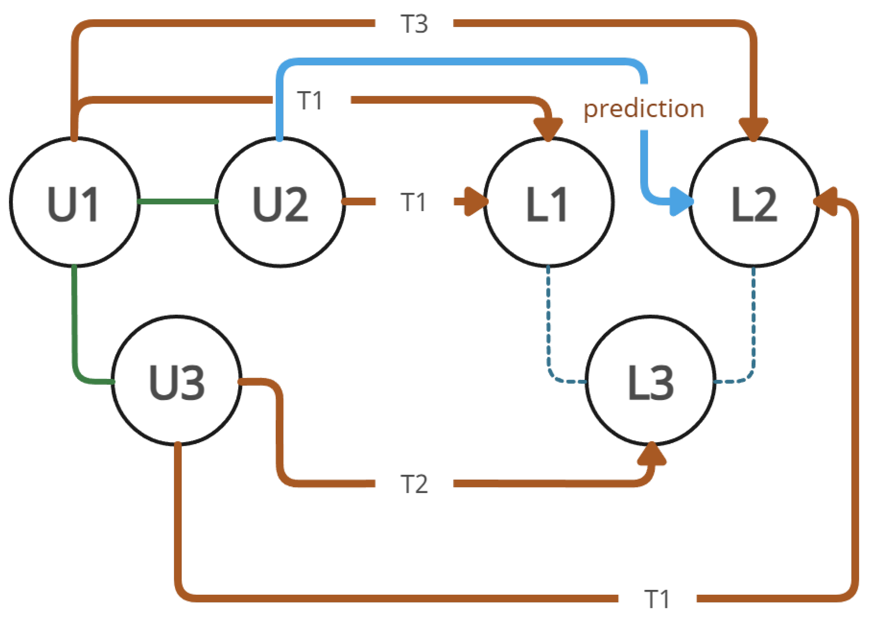
Figure 1 shows an example of a simple LSBN. User 1 (U1) is friends with User 2 (U2) and User 3 (U3). The first two users visited Location 1 (L1) in the same Time Period, U1 also visited L2 in Time Period 3 (T3), and U3 visited L3 in Time Period 2 (T2). L3 is close to L1 and L2. However, the latter are far from each other. Analyzing U2, the algorithm takes into account all nearby locations, which include L2 and L3, whereas L1 is left out since it is out of range. By calculating the embeddings, it ranks the locations that are most probable for U2 to visit, ranking L2 first and L3 second, due to the similarities with their connection’s preferences. As such, the algorithm predicts that U2 will visit L2 and recommends this location.

In this section, we describe the definition of the problem in detail and present the fundamental knowledge related to our research. In

Table 1. Frequently used symbols.

Symbol	Description
$\mathbf{U},\mathbf{L},\mathbf{C}$	set of users $\mathbf{U}$ = $\{u_1,\dots ,u_n\}$,
	set of locations $\mathbf{L}$ = $\{l_1,\dots ,l_m\}$,
	set of check-ins $\mathbf{C}$ = $\{c_1,\dots ,c_o\}$
$c_u$	user’s check-in
$e_{i,j}$	edge between two nodes
$\mathcal{E}$	set of edges $e_{i,j}$ over each graph
k	graph hop depth

, we list the frequently used symbols used throughout the article. The most fundamental definitions are as follows:

Definition 1.

(POI): This is a location in which users checked in. A POI is represented as a tuple: $<l_{id},longitude,latitude>$. Many different locations may share the tuples as they may belong in the same building; the location’s id, however, is different.

Definition 2.

(Check-in): This is a self-reported visit made by user u to location l at time t and is represented as a tuple: $c_i=<u,l,t>$. A check-in is made by only one specific user but one user may make multiple check-ins at the same location at any given time.

Definition 3.

(User–User Graph): This is a unipartite, undirected graph that describes the connection between the users. In social networks, this translates to each user’s friends.

Definition 4.

(User–POI Graph): This is a weighted undirected bipartite graph where each edge describes check-in c performed by user u at location l. Each edge starts with a weight of 1 and its weight is increased by 1 for each additional check-in the user makes in the future.

Definition 5.

(Location Map): This is an undirected unipartite graph depicting the POIs in a similar fashion to a map. Each location l is connected to all locations that are within a specific distance range. This essentially builds a tree-map of locations based on their proximity to one another. A small range includes nearby locations such as those in malls or similar venues and also locations within a reasonable walking/driving distance from each other. Venues too far apart do not have a link between them as they are considered too far apart for the user to change their preferred go-to location.

Definition 6.

(Streaming Recommendations): This is the prediction of the POI recommendation made by analyzing each incoming edge (or batch of edges $\mathcal{E}$) and then handling the update of the graphs, embedding and recommendation method accordingly. The latest actions of the user weigh more heavily on the recommendation process as stated in Definition 4.

Definition 7.

(Accuracy Threshold): This is the real-time prediction accuracy limit in the last $c_u$ check-ins on the current $\Delta T$ time-frame. Should the accuracy fall below the limit of the algorithm, the embeddings should be built from scratch; otherwise, they should be updated according to the updated graph that denotes the changes made since the time the embeddings where last built.

4. The Proposed Approach

In this section, we present the functionality of our algorithm. We start by explaining how we handle the initial multipartite graph and extract the initial embeddings. Then, we analyze the streaming process of handling new data and updating the aforementioned embeddings according to the new trends, and finally, we present the method of producing personalized recommendations.

First, we analyze the raw data set and extract the useful information, which includes the user friendship network (user–user), the visits of each user (user–location) and the time they were performed.

The check-ins are ordered by time. Each check-in is represented by its location coordinates, timestamp, and associated user. The data set is then split for the training and the test set. From the training set, we then extract the appropriate graphs described in Section 3.

4.1. Learning Embeddings of a Multipartite Graph

From the previous steps, we produce graphs for each of our networks. To unify the networks and transform them into a unipartite graph, we create new node identifiers for every entry, so that each node of every graph is now similar to the others. As such, instead of dealing with a multipartite graph, we now have a single unipartite graph to work with.

Table 2. Node conversion example.

Node Name	Node Connections
User 1 → 1	User 2, Location 1 → 2, 3
User 2 → 2	User 1 → 1
Location 1 → 3	User 1 → 1

shows an example with a bipartite graph consisting of three nodes where User 1 is connected to both User 2 and Location 1. The algorithm re-identifies the node names from 1 to 3 and translates them, respectively, transforming the network effectively into a unipartite graph.

To compute the embeddings, we use Gaussian random projection; we let $\mathbf{R}\in {\mathbb{R}}^{N\times d}$ with each element of $\mathbf{R}$ follow an independent and identically distributed Gaussian distribution $\mathbf{R}(i,j)\sim \mathcal{N}(0,\frac{1}{d})$. $\mathbf{S}$ is defined as high-order proximity with $w_0,w_1\dots w_q$ being the weights. The adjacency matrix is defined as $\mathbf{A}$ and $\mathbf{I}$ is the initial Gaussian Random Matrix. The embeddings are computed by the following matrix product:

$$\begin{array}{c}\hfill \mathbf{M}=\mathbf{S}·\mathbf{R}=(w_0\mathbf{I}+w_1\mathbf{A}+w_2{\mathbf{A}}^2+\dots +w_q{\mathbf{A}}^q)\mathbf{R}\end{array}$$

(1)

The outline of this process is shown in Algorithm 1. After we initialize the Gaussian Random Matrix, we form its depth by modifying the values according to the adjacency matrix. Finally, we build the embeddings by scaling each depth to its respective weight value.

Algorithm 1 Embedding Calculation
Require: Adjacency matrix A; embedding dimension d; weights W
Ensure: Embedding table M
1: Sample $R_0\leftarrow A\times d$	▹ Gaussian Random Matrix
2: for $i\leftarrow 1$ to $W.size$ do	▹ For every order defined by W
3:     $R_i\leftarrow A·R_{i-1}$	▹ Propagate one order
4: end for
5: Initialize $\mathbf{M}$ as a $A\times d$ zero matrix.
6: for $i\leftarrow 0$ to $W.size$ do	▹ Weighted sum of orders
7:     $\mathbf{M}\leftarrow \mathbf{M}+W_i·R_i$
8: end for
9: return $\mathbf{M}$

4.2. Streaming Recommendations

The test set is now inserted in batches. As described in Algorithm 2, for each entry, the algorithm produces recommendations on the existing embedding, noting the accuracy of each recommendation. To further improve the speed, only locations located at a distance of about 500 m from the user are considered for the recommendation process. We define the user’s location as the location of the POI where they checked in. After processing B entries, the algorithm updates the embedding tables using the data collected up to this point. After updating the embeddings, the algorithm continues the same process for the next B entries until the data set is covered. We also implement a checking mechanism, such that if the accuracy of the last recommendation is high, an update to the embeddings is considered counter-productive and as such, the algorithm delays the computation of the new embeddings until the accuracy falls below the specified threshold.

Algorithm 2 Recommendation evaluation
Require: Test check-in set C; embeddings M; batch size B; performance threshold τ
Ensure: Final results list R
1: Construct location network $LN$ from location coordinates	▹ Spatial index/proximity graph
2: Build network tree G
3: $G^{\prime }\leftarrow \varnothing$	▹ Accumulated graph changes
4: $R\leftarrow \left[\right]$	▹ Initialize results
5: for $i\leftarrow 0$ to $\left|C\right|-1$ do	▹ For every new check-in $c_i\in C$
6:     LNi ← NearbyLocations$(LN,c_i)$	▹ All locations within proximity
7:     ${\mathbf{M}}_{u_i}$ ← UserEmbedding$(\mathbf{M},c_i)$
8:     ${\mathbf{M}}_{L{N}_i}$ ← LocationEmbeddings$(\mathbf{M},L{N}_i)$
9:     $Rank\leftarrow {\mathbf{M}}_{u_i}·{\mathbf{M}}_{L{N}_i}^{\top }$	▹ Similarity scores
10:     Sort $Rank$ in descending order
11:     $Result$ ← FindRank$(Rank,c_i)$
12:     Append $Result$ to R
13:     $G^{\prime }$ ← AddEdge$(G^{\prime },c_i)$	▹ Add new check-in edge(s)
14:     if $(imodB=0)$ and (Perf$\left(R\right)<\tau$) then	▹ Decision to update
15:        M ← StreamingNEUpdate$(\mathbf{M},G^{\prime })$
16:        $G^{\prime }\leftarrow \varnothing$
17:    end if
18: end for
19: return R

4.3. Updating Embeddings

In the update process, we take into account the distance in the connection between user and location nodes in the graph. Instead of recomputing the whole embedding table $\mathbf{M}$ from scratch, we work on a subset of it, since the nodes that are many edges away, or not connected at all, will not be affected significantly (or at all) by the insertion of an edge between a user and a location. In a real-life scenario, we could say that the activity of a user in Germany will not affect a user in Sweden and vice versa; however, it will affect the users that are in close proximity to the user.

For the update process, we only take the rows of the embeddings that contain the original nodes that changed along with their neighbors $\mathbf{N}$ in depth k, as described in Algorithm 3. Changes to the embeddings $\mathbf{M}\in \mathbf{N}$ are computed using the following formula, where $\mathbf{A}$ is the weighted graph:

$$\begin{array}{c}\hfill \Delta {\mathbf{M}}_i=\mathbf{A}·\Delta {\mathbf{M}}_{i-1}+\Delta \mathbf{A}·{\mathbf{M}}_{i-1}+\Delta \mathbf{A}·\Delta {\mathbf{M}}_{i-1}\end{array}$$

(2)

A normal matrix factorization algorithm has a complexity of $\mathit{O}\left(n^3\right)$ in an $n\times n$ matrix. In our case, it is $\mathit{O}\left(n^2\right)$ since the size of the embeddings is 128 and can be considered as a constant. Decreasing the size of a table by a magnitude of one results in a computation time of a magnitude of two. Therefore, by decreasing the size of the embedding tables, taking into account the affected nodes and their neighbors in depth k, the execution time is reduced significantly, making the update procedure feasible in a streaming environment. The time savings for different data set sizes is further analyzed in Section 5.4.

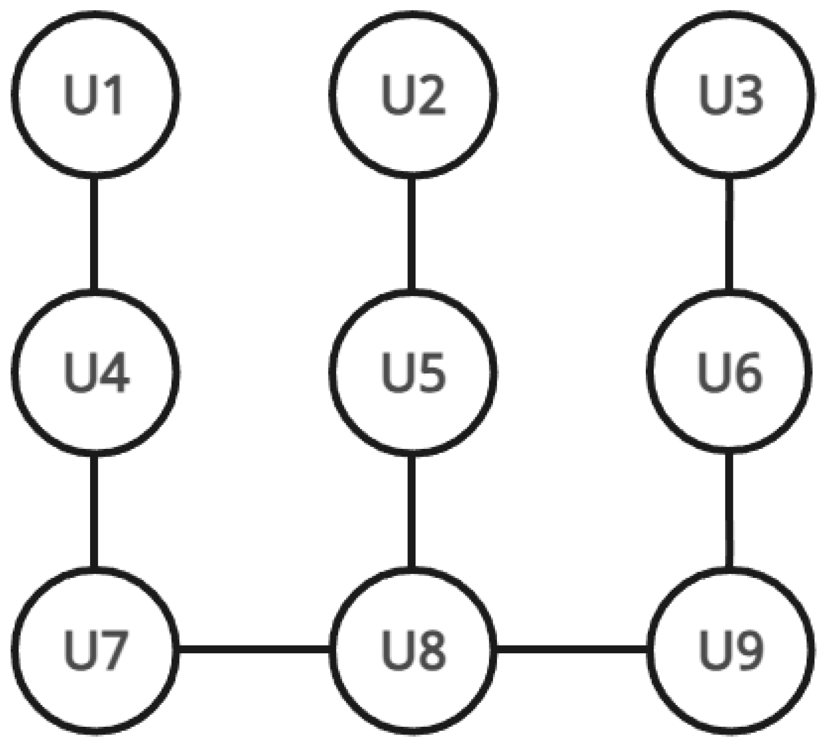
In Figure 2, we show an example graph of a user graph and the user’s respective embeddings in

Table 3. Example embeddings.

Embeddings
u1	${\mathbf{M}}_{u1,1},{\mathbf{M}}_{u1,2}\dots {\mathbf{M}}_{u1,d}$
u2	${\mathbf{M}}_{u2,1},{\mathbf{M}}_{u2,2}\dots {\mathbf{M}}_{u2,d}$
u3	${\mathbf{M}}_{u3,1},{\mathbf{M}}_{u3,2}\dots {\mathbf{M}}_{u3,d}$
u4	${\mathbf{M}}_{u4,1},{\mathbf{M}}_{u4,2}\dots {\mathbf{M}}_{u4,d}$
u5	${\mathbf{M}}_{u5,1},{\mathbf{M}}_{u5,2}\dots {\mathbf{M}}_{u5,d}$
u6	${\mathbf{M}}_{u6,1},{\mathbf{M}}_{u6,2}\dots {\mathbf{M}}_{u6,d}$
u7	${\mathbf{M}}_{u7,1},{\mathbf{M}}_{u7,2}\dots {\mathbf{M}}_{u7,d}$
u8	${\mathbf{M}}_{u8,1},{\mathbf{M}}_{u8,2}\dots {\mathbf{M}}_{u8,d}$
u9	${\mathbf{M}}_{u9,1},{\mathbf{M}}_{u9,2}\dots {\mathbf{M}}_{u9,d}$

. If we are to update User 8 with depth 1, then only that node and Users 5, 7 and 9 will be taken into account. With depth 2, Users 1 and 3 will also be considered, and so on. In this way, we deal with a significantly smaller subset of embeddings $\mathbf{M}$ that affect the nodes at a depth that significantly affects the closely connected nodes, while the distant nodes remain unaffected.

Algorithm 3 Dynamic embedding update
Require: Current embeddings M; graph G; weights ${\alpha }_n$; update set $G^{\prime }$; neighborhood depth k
Ensure: Updated embeddings ${\mathbf{M}}^{\prime }$
1: $N\leftarrow \varnothing$	▹ Node set to update
2: for all $g\in G$ do
3:     $N\leftarrow N\cup \left\{g\right\}$	▹ Add node
4:     neighbors ← FindNeighbours$(G,g,k)$	▹ Depth-k neighborhood
5:     $N\leftarrow N\cup \mathit{neighbors}$	▹ Add neighbors
6: end for
7: Initialize ${\mathbf{M}}^{\prime }$ as subset of $\mathbf{M}\in N$	▹ Keep only embeddings for nodes in N
8: ${\mathbf{M}}_0^{\prime }\leftarrow {\mathbf{0}}^{N.size\times d}$	▹ Zero matrix
9: for $i\leftarrow 0$ to q do	▹ For every embedding order/depth
10:     Compute $\Delta {\mathbf{M}}_i$ using Equation (2)
11:     ${\mathbf{M}}_i^{\prime }\leftarrow {\mathbf{M}}_i+\Delta {\mathbf{M}}_i$
12: end for
13: ${\mathbf{M}}^{\prime }\leftarrow {\alpha }_0{\mathbf{M}}_0+{\alpha }_1{\mathbf{M}}_1+\dots +{\alpha }_q{\mathbf{M}}_q$
14: return ${\mathbf{M}}^{\prime }$

4.4. Handling Cold Start

The cold-start phenomenon appears when a new node $g\notin G$ is created from a new edge $e\notin G$. In our algorithm, that means that a new user enters the network and makes their first check-in, or an existing user makes their first check-in at a previously unknown location. A cold start can be further extended to new check-ins from users with few friends and check-ins at locations that have few check-ins, in other words, on nodes that we have very little information about.

We solve the cold-start problem by connecting the new node to pre-existing ones. For the new user nodes, the user is connected with friends who are already connected with their friends, giving us context as to what group the new user belongs to. The new locations are related to other nearby locations, and as a user connects to them, they immediately gain the user’s connections as 2-depth neighbors. In addition, as previously analyzed in Section 4.3, each time a node is updated, we also update its neighbors N in depth k. That means that a new node will be updated each time there are new edges within its k-hop neighborhood; it will be updated even if there are no new direct connections to itself. As such, even a completely new location will be quickly integrated into our existing network of information and will be personalized more quickly as we exploit its neighbors for collateral information.

4.5. Producing Recommendations

The predictions are computed using the embedding vector of user u, multiplied by the transpose of the embedding matrix of nearby locations ${\mathbf{M}}_L$, as described in Equation (3). We define nearby locations as the location of the POI the user actually visited and all other locations within a specific range R of that location. This results in a series of values $V_u$, which denote the preferential personalized scores for each location for the specific user.

$$\begin{array}{c}\hfill V_u=\mathbf{u}·{\mathbf{M}}_L^T\end{array}$$

(3)

By ordering $V_u$ in ascending order, we get the list of locations the user will probably visit. The rank of the location the user actually visits increases the respective $topK$ value. We save the top 1, top 5, top 10, top 25 and top 50 results, denoting the top 10 as “first-page results”, and the rest reveal useful information about the prediction process we analyze in Section 5.

5. Performance Evaluation

In this section, we provide details on the performance of the proposed methodology along with the data that was used for evaluation. We also analyze the different results obtained by changing the values of the required parameters. The source code as well as links to the data sets that have been used can be found at https://github.com/thedx4/spoir, accessed on 12 February 2026.

5.1. Data Sets

In our experiments, we use three real-world data sets: (i) Foursquare (https://github.com/thedx4/spoir/tree/main/Foursquare, accessed on 12 February 2026), (ii) Weeplaces (https://github.com/mat-analysis/datasets/tree/main/mat/Weeplaces/Weeplaces%20original, accessed on 12 February 2026) and (iii) Gowalla (https://github.com/thedx4/spoir/tree/main/Gowalla, accessed on 12 February 2026). From each data set, we extract the user–POI check-ins along with the friendship network, whereas any additional information is discarded.

Table 4. Characteristics of data sets.

Data Set	Check-ins	Friend Network	Time-Span (Months)
Foursquare	483,813	32,511	42
Weeplaces	7,658,368	119,930	91
Gowalla	36,001,679	4,418,339	31

shows the total number of check-ins, friendship connections, and the time-span from the first check-in to the last one.

The Foursquare data set is ideal for testing our algorithm on a small-scale network as the pre-processing procedure and the evaluation method are both relatively fast, while differences between methods can be clearly distinguished. Additionally, the Weeplaces data set provides a larger time-span of check-ins on which we also test the effectiveness of our method over a large time period. Lastly, the Gowalla data set features an enormous amount of data which allows us to stress-test our algorithm against heavy load, which is also expected from a large-scale social network.

5.2. Evaluation Methodology

For each data set, we sort the data by check-in timestamp in ascending order to simulate the chronological arrival of user interactions and we use 80% for the initial training and 20% for the testing phase. For the friendship network, since there is no indication of where an edge is created, we include it in its entirety from the beginning. During the testing phase, each check-in is handled one by one as a real-world simulation method. The different areas of the results are categorized as follows:

• Automatic Updates: The algorithm decides on its own when it is time to build the embeddings from scratch. By default, this occurs when the accuracy falls below 55% on a sample size of at least the latest 100 entries. This greatly saves time in the long run as updating from scratch too often greatly affects the execution time and provides little to low increase in accuracy as the results show. We also compute the root mean square error between the embeddings made from scratch and the updated embeddings to further prove this point.
• Embedding Entries: The algorithm decides whether to update the embeddings or build them from scratch every N entries. The greater the number, the better the execution time is, since there is no time consumed by altering the embeddings altogether. This is useful especially on larger networks, where there are multiple entries even every second that should not be immediately calculated into the embeddings as they will not affect the predictions much.
• Neighbor Depth: In the update procedure, we update the affected nodes and their neighbors with depth k. Naturally, as we increase the depth, we increase the number of affected nodes. However, since we already include in the calculations more than two affected nodes, we do not go further than a depth of two, since that would exponentially increase the node count and possibly even result in the greater part of the whole graph. This becomes more evident as we constantly discover more and more connections between users and locations.
• Location Range: We define the maximum range R of locations from the user that we will take into account for the recommendation process. We start from the recommended distance of around 500 m from the user and we go as far as 4 km. Of course as the difference increases, so does the user’s choices; however, since people do not often travel very large distances in order to visit locations, we opt to use a reasonable distance within a common municipal area.

In each evaluation, we take into account the following parameters:

• Accuracy: The accuracy is defined as top@n and is calculated as $Accuracy@n=TruePositive@n/TotalRecommendations@n$ and presented as a percentage (%). For a top@n to be counted, there has to be approximately $2n$ locations in the R vicinity of the user. A $TruePositive@n$ is counted when the user visits a location that appears in the top-n recommended locations during the corresponding evaluation instance.
• Average Location Number: We note the average location number to further point out the accuracy since achieving top@n in larger location areas is more challenging, especially on larger social network platforms.
• Execution Time: One of the most critical parameters is the processing time in the streaming procedure. In order to maintain a reasonable execution time, we take into account the embedding build time both from scratch and for an update.
• RMSE: Root mean square error dictates the differences between the embeddings built from scratch and the updated embeddings, where a small difference in accuracy denotes a big difference in execution time. It is calculated as shown in Equation (4), where ${\mathbf{M}}_u$ is the embeddings we apply our update method to and ${\mathbf{M}}_s$ is the embeddings we calculate from scratch. The lower the RMSE is, the more similar the embeddings are.

$$\begin{array}{c}\hfill RMSE=\sqrt{{\displaystyle \frac{1}{n}}{\displaystyle \sum _{i=1}^n}{({\mathbf{M}}_u-{\mathbf{M}}_s)}^2}\end{array}$$

(4)

Unless otherwise specified, we use the following parameters during the testing phase: The range is 500 m from the checked-in location. Batch size is set to 10,000 check-ins before changing the embeddings. The top-10 accuracy threshold over the last 100 check-ins is set to 55% in order to decide whether to update the embeddings or build them from scratch. Neighbor hops are limited to two. For the embedding algorithm, we use a weight of 3:1, 0.1, 0.01, and 0.001 respectively, and the depth of the embedding table is set to 128.

In the next paragraphs, we discuss the performance fluctuation over the data sets and the parameters used to show the process we followed to reach the aforementioned numbers, which we consider to be optimal in our evaluation procedure.

5.3. Streaming vs. Static

Traditionally, the data set is processed from the beginning as a whole, and as such, the embeddings are generated each time we make recommendations. This procedure, while maintaining high accuracy, is detrimental in terms of execution time and is only useful and practical in theoretical situations. Real-time processing of data requires fast data analysis as incoming data is constantly being generated by the network’s users and the algorithm needs to keep up with recent trends to provide up-to-date recommendations.

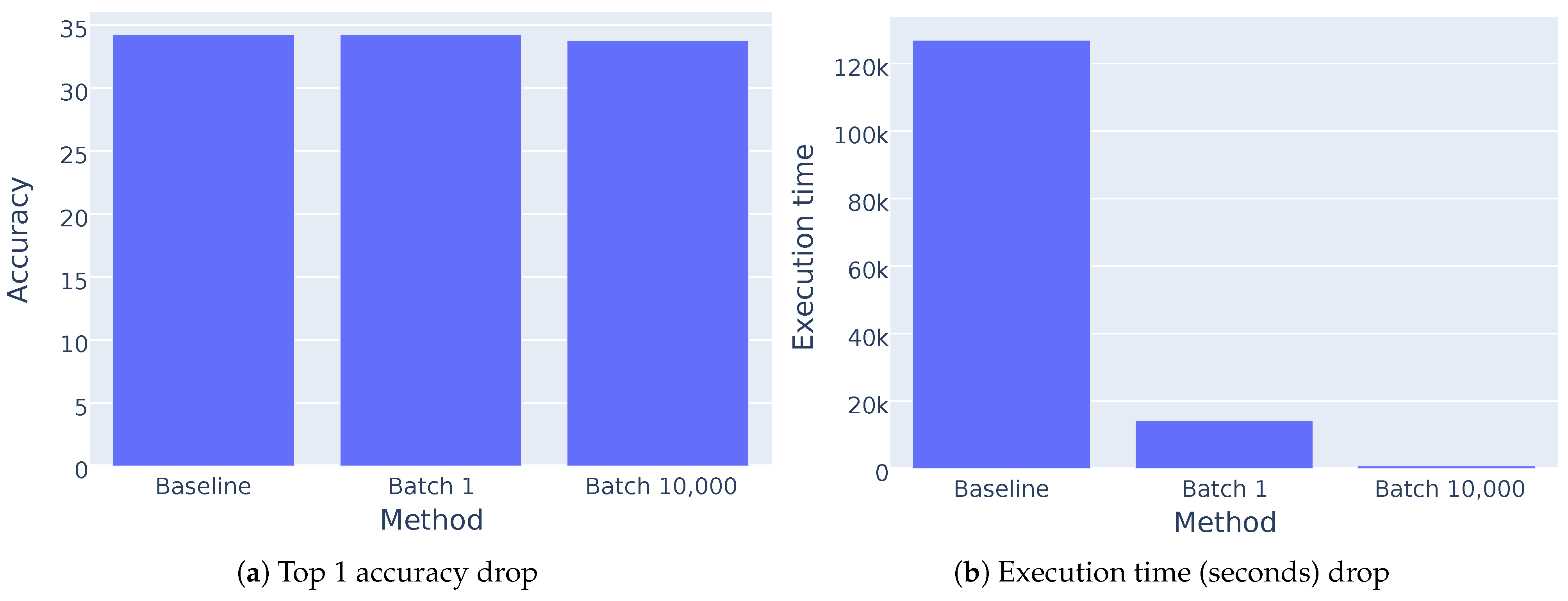
In this section, we compare our algorithm against the conventional approach, which rebuilds the embeddings from scratch after each new insertion. Figure 3a presents the Top-1 accuracy drop across different batch sizes on the Foursquare data set. Although a slight decrease in accuracy is observed, Figure 3b demonstrates that the proposed update method achieves orders-of-magnitude reductions in execution time. Therefore, the marginal loss in accuracy is substantially outweighed by the significant computational gains.

As described in Section 4.3, instead of taking into account the whole graph in order to build the embeddings, we take a small subset of it ${\mathbf{M}}_k$, which is the sum of the affected nodes along with their neighbors in depth k. This exponentially decreases the matrix size and therefore the total execution time for the process of updating the new embeddings. As we hypothesized, the users and locations that are a greater distance from the area of activity are less likely to be affected and as such, we do not take them into account for the update process.

5.4. Results for Different Batch Sizes

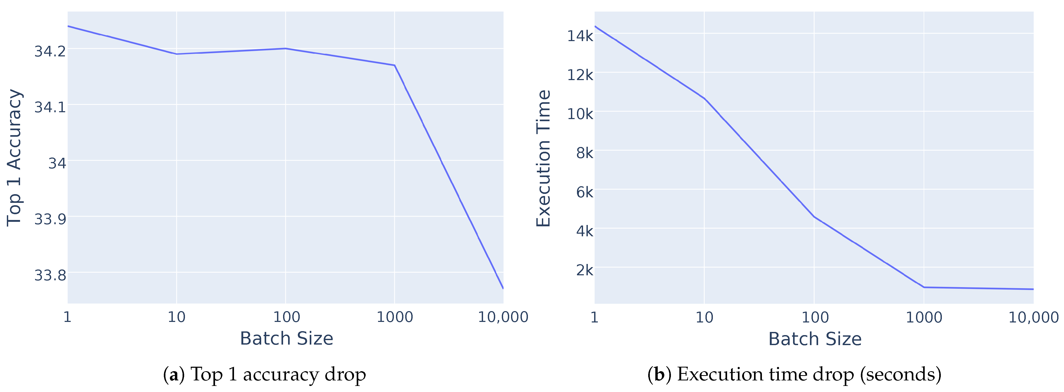
We explore several batch sizes to study the differences between constantly updating the embeddings and sparse updating. We start by using a batch size of 1 and increase the size by a magnitude until we reach 10,000 entries. As we can see in Figure 4a, the accuracy does not drop significantly as the size increases. To show the impact on execution time, we include Figure 4b, and we observe a significant drop in the overall computation time.

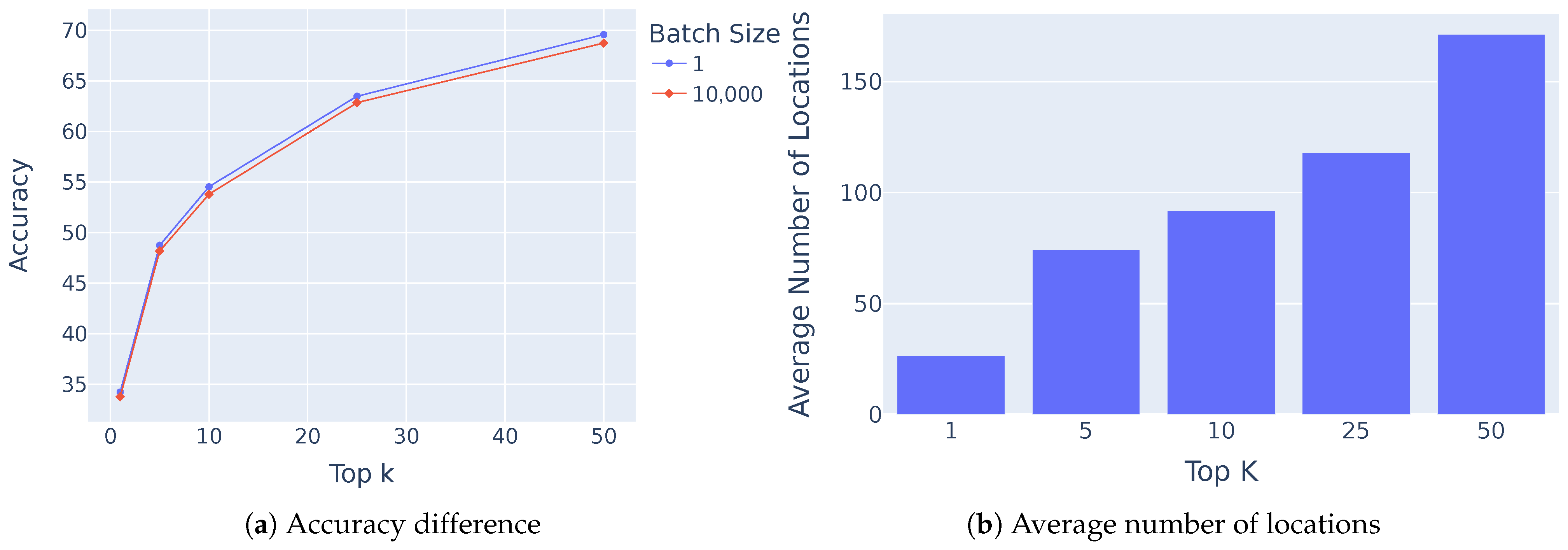
To further investigate the accuracy and efficiency of the algorithm on batch sizes, we include Figure 5, in which we show the comparison between the accuracy according to the batch size in Figure 5a and the average number of locations that the program has to make the recommendations from in Figure 5b.

Table 5. Average RMSE statistics for Foursquare.

Embedding Building Method	Execution Time (s)
From scratch (1 check-in)	1.92
Update (1 check-in)	0.18
From scratch (all check-ins)	126,963
Update (all check-ins—Batch 1)	14,364
Update (all check-ins—Batch 1000)	966
RMSE error (Batch 1): 0.0035
RMSE error (Batch 1000): 0.3404

shows the embedding build time, the total execution time and the average root mean square error (RMSE) (https://en.wikipedia.org/wiki/Root-mean-square_deviation, accessed on 12 February 2026) on the Foursquare data set. We first run the baseline algorithm where we update the embeddings from scratch each time a new check-in comes in. Then, we proceed to run the same experiment where we update the embeddings every check-in. Finally, we test it again where we update the embeddings every 1000 check-ins.

For this testing phase, each time the embeddings are updated, we re-run the process by updating them from scratch, in order to calculate the RMSE for that specific batch. As we see from the results, the error is quite low, while the execution times are magnitudes lower, effectively reducing them from more than a day to around 15 min.

Although updating the embeddings while also increasing the batch size greatly affects the execution time, there is a point where the time saved compared to the accuracy drop reaches a critical point. As we observe in Figure 4, for batch sizes of 1000 and 10,000, the time saved is minimal while the accuracy begins to drop significantly. At that point, we can safely state that for the Foursquare data set, the optimal batch size should be around 1000 since our results show that the critical point is reached at this specific value.

To further evaluate the time saved between building the embeddings from scratch and updating them, we further test our algorithm’s speed on the Gowalla and Weeplaces data sets. We test the times for building the embedding tables from scratch and for updating them for every incoming check-in. We calculate the average value of the times, as these differ for the check-ins denoted by the neighboring affected nodes. As

Table 6. Average execution time statistics on Weeplaces and Gowalla.

Embedding Building Method	Execution Time (s)
From scratch (Gowalla)	113.84
From scratch (Weeplaces)	22.01
Update (Gowalla)	1.09
Update (Weeplaces)	9.01

shows, the difference between updating check-ins and building them from scratch is magnitudes apart.

As shown when we previously analyzed the characteristics of the data sets in Table 4, the Gowalla data set is about two orders of magnitude larger than the Foursquare one, which is ideal for illustrating the difference in the execution time depending on the abundance of data.

5.5. Results for Different Numbers of Hops

As we previously analyzed, altering the number of hops that we search for the neighbors of the affected nodes greatly affects the execution time. As the size increases, the number of nodes affected increases exponentially, resulting in the update time getting closer to the time for if embeddings are made from scratch.

Table 7. Results vs. number of hops.

Result	Depth 1	Depth 2
Mean Embedding Time (s)	0.135	0.174
Total Execution time (min)	163	205
Top 1 accuracy	32%	39%

shows the difference in execution time and accuracy between 1 and 2 hops.

5.6. Results for Larger Data Sets

In this section, we explore the efficiency of the algorithm in more diverse and bigger data sets and as such, they are compared on several factors. As the data sets differ greatly as previously discussed in Section 5.1, we can better understand the effectiveness of the update procedure. Also, on bigger data sets, the runtime difference between the update procedure and the building of embeddings from scratch is better shown on dense networks where the nodes and edges make analyzing the whole data set too expensive regarding computer resources and time, whereas updating a small portion of it—even a dense one—is significantly more efficient.

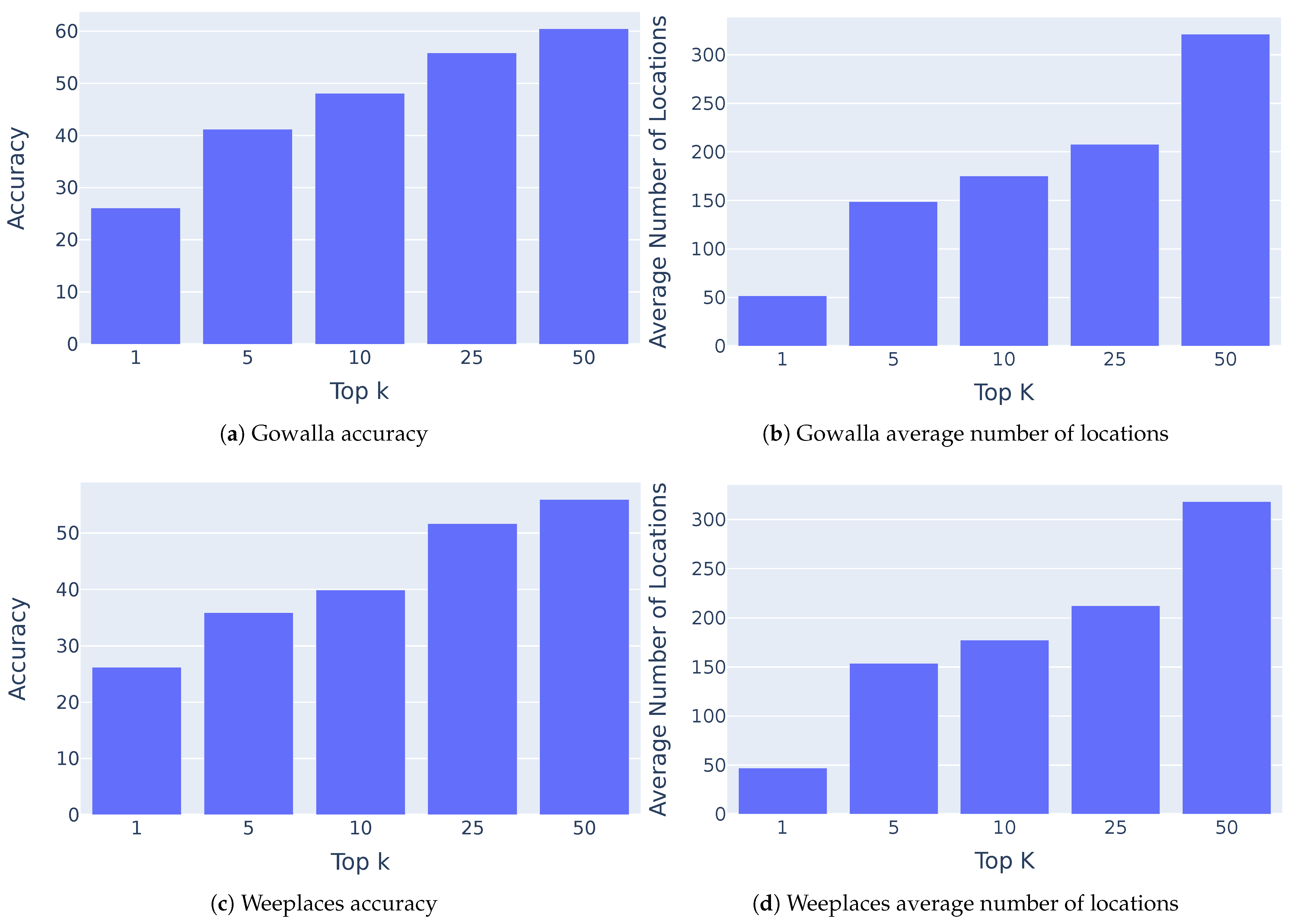
As we mentioned earlier, we list the accuracy and average number for each data set and we present them in Figure 6. We notice that the average locations are at least a magnitude bigger in size in comparison to our top recommendations, and yet we maintain a high accuracy ratio. The results confirm our initial hypothesis of the time saved in bigger data sets; however, what we consider true success is the minimal loss in accuracy, even when comparing Top-K results. Compared to Figure 5b, Gowalla and Weeplaces contain at least an order of magnitude more locations, which explains the observed differences in performance. Despite this scale gap, Gowalla and Weeplaces share similar structural characteristics, resulting in comparable performance behavior. Importantly, achieving high Top-k accuracy on data sets with substantially larger location coverage demonstrates the robustness of the method under increased data complexity.

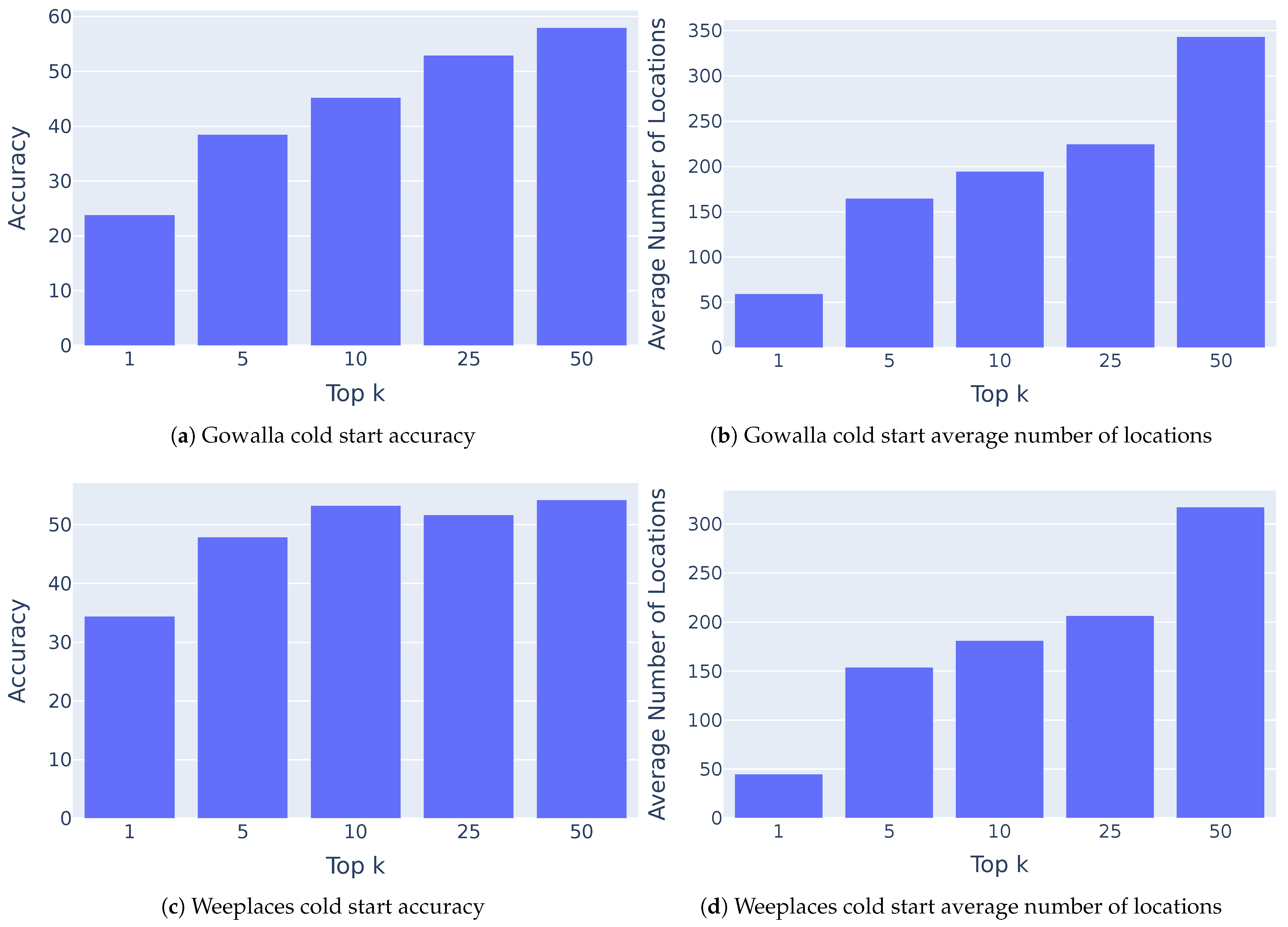
5.7. Evaluation of Cold Start

A cold start is a problem in any prediction model. New locations, users and other related data for which the network contains little or no information contribute to the cold start problem. We tackle this issue by integrating the new node into pre-existing ones and updating them according to their neighbors, as described in detail in Section 4.4.

Figure 7 shows the accuracy and the average number of locations in the two largest data sets, i.e., Gowalla and Weeplaces. The inclusion of the new locations also contributes to an increase of the average number of locations each time the algorithm generates a prediction for a specific area. As we include the cold start handling process for users and locations into our algorithm, we observe a drop in accuracy as is expected, since adding the new locations and users makes it challenging for the algorithm, as even if the process of including the new nodes into the information network is quick, it still takes some time for them to be fully integrated. However, we notice less of a drop in the Top 5 and Top 10 categories of results, which means that even with this drop, we still maintain high accuracy for new users and new locations.

6. Conclusions

Streaming recommendations and updating users’ preferences in real time is crucial to modern society as technology and online users constantly increase and data flow also increases as a result. Conventional methods of predicting user activity become obsolete and inefficient, with their execution time increasing dramatically due to the increased traffic flow and activity. Real-time updates of user activity provide us with an almost immediate reaction to the user’s latest movements, making predictions more accurate and realistic.

In this work, we propose a novel approach for the selective update of the embeddings used in user recommendation, significantly reducing the number of affected nodes and edges, which leads to more efficient computation times, while maintaining high accuracy.

As the results showed in Section 5.3, our algorithm outperforms conventional methods in terms of execution time, with a minimal reduction in accuracy. Especially in larger networks, where the network connections between users and locations as well as the increased number of users and activity increase exponentially, updating only specific parts of the embeddings offers a dramatic difference in execution time, resulting in characterizing the update method as efficient and effective, as shown in Section 5.6. There are several interesting research directions for future work.

• One way to further improve performance is the use of parallel and distributed versions of the algorithm. In this way, we will be able to cope with the increased processing load posed by the size of the networks and also the high arrival rate of incoming data.
• Incorporating contextual information, such as demographic attributes and user group characteristics, has been shown to improve the performance and fairness of POI recommendation models, as mobility patterns often vary across different user populations [17,18]. Extending the proposed approach to integrate demographic signals or group-aware representations represents a promising direction for improving personalization and capturing heterogeneous user behavior.
• Another interesting direction is the support of a sliding window streaming model, where a decay process may be applied, turning some information to obsolete after a period of time. The challenge in this case is that we have not only insertions due to new information but also deletions due to the expiration of already existing data.
• Finally, it would be interesting to study techniques based on Graph Neural Networks (GNNs) and how they can help in updating the embeddings in the streaming scenario more efficiently.