Robustness of Circular Neighbor-Balanced Designs with Correlated Data and Missing Observations

Abstract

This paper examines the robustness of circular neighbor-balanced designs (CNBDs), a significant issue in experimental design when observations are missing and errors are correlated. Treatments may affect not only the designated unit but also its adjacent units, hence complicating the estimation of treatment effects in assessments utilizing adjoining plots. This paper proposes to measure the robustness of CNBDs by analyzing two models, one with and one without block effects, under four correlation structures: MA(1), NN, AR(1), and ARMA(1,1). It considers the robustness of these designs in terms of A- and D-efficiencies for direct and neighboring effects. We observed that designs with lower correlations between observations also yield smaller efficiency losses when data is missing, resulting in more robust designs. Some neighbor designs offer strong performance with missing observations and correlated errors, minimizing efficiency losses. This study contributes to experimental design for CNBDs under challenging conditions for missing observations and correlated data—that is significant.

1. Introduction

In both natural and simulated experiments, researchers typically expect that the performance of all input variables will be optimal and yield reliable results. However, this expectation is often unmet, as many treatment combinations fail to perform as expected due to unforeseen factors, particularly in field conditions where variability is difficult to control. Several factors can compromise the quality and efficiency of an experiment, including missing data in blocks or treatments, outliers, irregular patterns, correlated errors, unequal error variances, and other model misspecifications. Experimental processes become more complicated in many cases due to issues with compromise treatments and external disturbances. Missing observations constitutes a particularly important problem because they can affect the analysis and reduce the reliability of the results.

Box [1] introduced the concept of robustness in statistical analysis in the context of the t-test for two samples with uncorrelated data and missing observations. Mahoney [2] later revisited the topic in relation to block design with algorithms to resolve various correlated matrices and data compilations. Robustness denotes a method’s capacity to operate effectively despite the disruption of its foundational assumptions. A sound and reliable experimental design should be resilient to adverse effects from issues such as absent data, outliers, and model violations. In practical applications, experimental designs must exhibit resilience, allowing researchers to derive meaningful results despite suboptimal settings. This work concentrates on the resilience of circular neighbor-balanced designs (CNBDs) with correlated data and missing observations, building upon this fundamental concept.

The term “neighbor effect” refers to the phenomenon in which the response of an experimental unit is affected by the treatment applied to its neighboring plots. And the mechanism/arrangement utilized to allocate treatments to experimental units in such a manner that each experimental material receives a certain treatment an equal number of times as compared to a neighbor is called neighbor-balanced design. Neighbor-balanced designs ensure that treatment comparisons are minimally affected by neighboring plots. Rees [3] introduced the concept of neighbor designs and circular neighbor-balanced designs. According to Azais [4], using neighbor-balanced designs can make for bias due to neighbor effects being negligible.

Three effects are considered: (i) the direct effect of a treatment on the unit to which it is applied, (ii) the effect caused by a treatment exercised on a left-neighboring unit, or left-neighbor effect, and (iii) the effect due to a treatment applied to a right-neighboring unit, or right-neighbor effect [5]. The literature provides methods for constructing CNBDs and circular partially neighbor-balanced block designs for estimating direct and neighbor effects of treatments. Jaggi et al. [6] and Khalid et al. [7] presented some infinite series to develop first-order neighbor-balanced designs (NBDs) in linear blocks of three and four. They also developed generators through the method of cyclic shifts to construct minimal circular generalized neighbor designs in different size blocks of two and three and highlighted the preference for minimal neighbor designs due to their cost-effectiveness. However, constructing minimal circular neighbor designs may not be feasible in every case where v (the number of treatments) is even [8,9].

Optimality phases of complete block designs with interference effects arising from neighboring units up to a distance of two (first and second order) were illuminated, providing conditions of universal optimality for block design to estimate direct and interference effects [10]. Jeevitha and Santharam [11] studied the optimality of CNBDs for total effects with equal right- and left-neighbor effects in the model, and the errors were correlated. Optimal properties of some circular balanced block designs under a model with a first-order circular autoregression were discussed [12]. Kong et al. [13] studied circular designs under interference models, where a treatment allocated to a plot is also affected by neighboring plots (from one side, two sides or the previous one) within a block. They developed a design framework and examined optimal designs across the design space. Khodsiani and Pooladsaz [14] described optimal properties of some circular block designs under a model with circulant correlation.

Robustness for specific missed observations for neighbor-balanced designs was examined, and the information matrix for one missing observation of the resulting design for the direct treatment effects and its efficiency was derived. Robustness of the neighborhood balanced complete block design has also been studied when more than one observation is missing, with high efficiencies demonstrated in the robustness of the design against missing observations [15].

The universal optimality of the nearest-neighbor-balanced designs (NNBDs) was examined by Santharam and Ponnusamy [16], using first-order correlated models such as AR(1), MA(1), and ARMA(1,1). Tomar and Jaggi [17] studied the efficiency of neighbor-balanced block designs under AR(1) and nearest-neighbor (NN) correlated structures. With correlated observation errors, Jeevitha and Santharam [11] incorporated equal right- and left-neighbor effects into the CNBD model in addition to optimality for total effects. Other researchers have developed optimal or efficient circular balanced block designs in the context of different correlated structures in different ways [12]. Abeynayake et al. [15] investigated the robustness of neighbor-balanced block designs, given missing observations. If one observation is missing, however, there occurs the scenario examined here, and the robustness of universally optimal CNBDs is studied in the presence of correlated observations in this paper. In terms of A- and D-efficiencies, we assess the losses due to missing observations. A neighbor design is said to be robust if, under some defined correlation structure and correlation coefficient, when an observation is misestimated, it suffers minimal efficiency loss; considering the efficiencies of neighbor-balanced block designs, this focuses only on the AR(1) and NN correlated structures. Jeevitha and Santharam [11] studied the optimality of CNBDs for total effects, incorporating equal right- and left-neighbor effects in a model with correlated observation errors. Filipiak et al. [12] discussed optimal properties of circular balanced block designs under a circular AR(1) model, while other researchers have explored optimality and efficiencies using different correlated structures in different ways. Abeynayake et al. [15] addressed the robustness of neighbor-balanced block designs with missing observations.

In this paper, the robustness of universally optimal CNBDs is studied in the presence of correlated observations when a single observation is missing. We assess efficiency losses using A- and D-efficiency. Under a specified correlation structure and correlation coefficient, a neighbor design is considered robust if it incurs a small efficiency loss when an observation is missing.

Application of Neighbor Designs

Here we present some examples to demonstrate the application of neighbor designs. Let us consider a couple of examples to show the usefulness of the proposed design.

Example 1: In virology, the Ouchterlony gel diffusion test is a method used to study relationships within a group of viruses. It consists of an antiserum that diffuses through appropriate media (like an agar gel) and antigens (like viruses). Antigens are placed evenly spaced around an antiserum on circular plates to form the test’s circumference. At the intersections of the diffusion areas, a precipitate line is formed by the antiserum and two adjacent (neighboring) antigens if they share components. Then, the experimenter observes these lines. Every antigen must be present in every other antigen equally frequently to fully investigate the relationships within the set of antigens.

An early presentation of the notion of neighbor designs was that of [3]. It was described for this example as the following: v antigens settled in b circular plates having k antigens (not undoubtedly distinctive). Every antigen has r appearances (possibly in r distinct blocks) and is always next to another antigen at the same time. This illustration shows how to apply circular blocks and neighbor designs.

Example 2: In certain countries, terraces cut into hillsides provide agricultural land [18]. These terraces circle a hill in naturally occurring circular blocks. It is best to take the effects of nearby treatments into account when conducting an experiment using such blocks. Neighbor designs in circular plots are therefore highly advised in these circumstances.

The rest of the paper is structured as follows. Section 2 presents the models and the methodology used in this study. It covers various types of correlation structure and disturbance matrices [19]. Section 3 develops the theory of universal optimality models, and properties associated with neighbor designs are given. In Section 4, we develop optimality criteria with respect to A- and D-efficiency, respectively, which emphasizes the idea of loss in A- and D-efficiency parameter estimation within the properties of a good model. Section 5 contains important results utilizing models and efficiency criteria from the previous sections. The final section also contains some concluding remarks.

2. Models and Research Methodology

Consider the following linear models related to design d ∈ D having an interference (neighbor) effect:

Y_d = X_1,dθ₁ + X_2,dθ₂ + X₃θ₃ + ε

(1)

Y_d = X_1,dθ₁ + X_2,dθ₂ + ε

(2)

where ${\mathbf{X}}_{\mathit{i},\mathit{d}}\in {\mathbb{R}}^{\mathit{n}\times {\mathit{p}}_{\mathit{i}}}$ i = 1,2 the obvious matrices, depending on design, d; ${\mathbf{X}}_{\mathbf{3}}\in {\mathbb{R}}^{\mathit{n}\times {\mathit{p}}_{\mathbf{3}}}$ is the matrix independent of d. The vectors of related parameters are θ_i, i = 1,2, while the vector of nuisance parameters is θ₃. With E(ε) = 0 and var(ε) = σ²V, where V = I_b⨂W_k is a specific symmetric positive matrix and the W_k matrix represents the association between random errors within the blocks of size k, ε represents a vector of random errors. If W_k = I_k, as a result, V = I_n, and then the observations are uncorrelated.

The information matrix of a general linear model used to estimate the individual vector θ_i, i = 1,2,3 or to value the whole effect θ₁ + θ₂ under (1) and (2) is expressed as:

Y_d = X_dθ + ε

(3)

Given a design matrix X_d and a vector of parameters θ, the information matrix C_d is as follows, assuming that the observations are uncorrelated:

$${C_d=\mathbf{X}}_d^{\prime }{\mathit{X}}_{\mathit{d}}$$

Similarly, the complete information matrix for model (1) is

$$C_d=\left[\begin{array}{ccc}{\mathbf{X}}_{1,d}^{\prime }{\mathit{X}}_{1,\mathit{d}}& {\mathbf{X}}_{1,d}^{\prime }{\mathit{X}}_{\mathbf{2},\mathit{d}}& {\mathbf{X}}_{1,d}^{\prime }{\mathit{X}}_3\\ {\mathbf{X}}_{2,d}^{\prime }{\mathit{X}}_{1,\mathit{d}}& {\mathbf{X}}_{2,d}^{\prime }{\mathit{X}}_{2,\mathit{d}}& {\mathbf{X}}_{2,d}^{\prime }{\mathit{X}}_3\\ {\mathbf{X}}_3^{\prime }{\mathit{X}}_{1,\mathit{d}}& {\mathbf{X}}_3^{\prime }{\mathit{X}}_{2,\mathit{d}}& {\mathbf{X}}_3^{\prime }{\mathit{X}}_3\end{array}\right]$$

(4)

The joint information matrix for calculating the total impact (θ₁ + θ₂) can be derived in the following format:

$$C_d\left({\mathit{\theta }}_{\mathbf{1}},{\mathit{\theta }}_{\mathbf{2}}\right)=[A_{11}-A_{12}{A}_{22}^{-}{A}_{21}]$$

(5)

where in (5) the submatrices are defined below:

$$A_{11}=\left[\begin{array}{cc}{\mathbf{X}}_{1,d}^{\prime }{\mathit{X}}_{1,\mathit{d}}& {\mathbf{X}}_{1,d}^{\prime }{\mathit{X}}_{\mathbf{2},\mathit{d}}\\ {\mathbf{X}}_{2,d}^{\prime }{\mathit{X}}_{1,\mathit{d}}& {\mathbf{X}}_{2,d}^{\prime }{\mathit{X}}_{2,\mathit{d}}\end{array}\right]$$

$$A_{12}=\left[\begin{array}{c}{\mathbf{X}}_{1,d}^{\prime }{\mathit{X}}_3\\ {\mathbf{X}}_{2,d}^{\prime }{\mathit{X}}_3\end{array}\right], A_{21}=\left[\begin{array}{cc}{\mathbf{X}}_3^{\prime }{\mathit{X}}_{1,\mathit{d}}& {\mathbf{X}}_3^{\prime }{\mathit{X}}_{2,\mathit{d}}\end{array}\right], A_{22}={\mathbf{X}}_3^{\prime }{\mathit{X}}_3$$

$$C_d\left({\mathit{\theta }}_{\mathbf{1}},{\mathit{\theta }}_{\mathbf{2}}\right)=\left[\begin{array}{cc}{\mathbf{X}}_{1,d}^{\prime }{\mathit{X}}_{1,\mathit{d}}-{\mathbf{X}}_{1,d}^{\prime }{\mathit{X}}_3{\left[{\mathbf{X}}_3^{\prime }{\mathit{X}}_3\right]}^{-}{\mathbf{X}}_3^{\prime }{\mathit{X}}_{1,\mathit{d}}& {\mathbf{X}}_{1,d}^{\prime }{\mathit{X}}_{2,\mathit{d}}-{\mathbf{X}}_{1,d}^{\prime }{\mathit{X}}_3{\left[{\mathbf{X}}_3^{\prime }{\mathit{X}}_3\right]}^{-}{\mathbf{X}}_3^{\prime }{\mathit{X}}_{2,\mathit{d}}\\ {\mathbf{X}}_{2,d}^{\prime }{\mathit{X}}_{1,\mathit{d}}{-\mathbf{X}}_{2,d}^{\prime }{\mathit{X}}_3{\left[{\mathbf{X}}_3^{\prime }{\mathit{X}}_3\right]}^{-}{\mathbf{X}}_3^{\prime }{\mathit{X}}_{1,\mathit{d}}& {\mathbf{X}}_{2,d}^{\prime }{\mathit{X}}_{2,\mathit{d}}{-\mathbf{X}}_{2,d}^{\prime }{\mathit{X}}_3{\left[{\mathbf{X}}_3^{\prime }{\mathit{X}}_3\right]}^{-}{\mathbf{X}}_3^{\prime }{\mathit{X}}_{2,\mathit{d}}\end{array}\right]$$

To find information matrices for individual effects θ₁ and θ₂, again partitioning the joint information matrix C_d(θ₁,θ₂) as

$$C_d\left({\mathit{\theta }}_{\mathbf{1}},{\mathit{\theta }}_{\mathbf{2}}\right)=\left[\begin{array}{cc}A& B\\ C& D\end{array}\right]$$

$$A={\mathbf{X}}_{1,d}^{\prime }{\mathit{X}}_{1,\mathit{d}}-{\mathbf{X}}_{1,d}^{\prime }{\mathit{X}}_3{\left[{\mathbf{X}}_3^{\prime }{\mathit{X}}_3\right]}^{-}{\mathbf{X}}_3^{\prime }{\mathit{X}}_{1,\mathit{d}}$$

$$B={\mathbf{X}}_{1,d}^{\prime }{\mathit{X}}_{2,\mathit{d}}-{\mathbf{X}}_{1,d}^{\prime }{\mathit{X}}_3{\left[{\mathbf{X}}_3^{\prime }{\mathit{X}}_3\right]}^{-}{\mathbf{X}}_3^{\prime }{\mathit{X}}_{2,\mathit{d}}$$

$$C={\mathit{B}}^{\prime }={\mathbf{X}}_{2,d}^{\prime }{\mathit{X}}_{1,\mathit{d}}{-\mathbf{X}}_{2,d}^{\prime }{\mathit{X}}_3{\left[{\mathbf{X}}_3^{\prime }{\mathit{X}}_3\right]}^{-}{\mathbf{X}}_3^{\prime }{\mathit{X}}_{1,\mathit{d}}$$

$$D={\mathbf{X}}_{2,d}^{\prime }{\mathit{X}}_{2,\mathit{d}}{-\mathbf{X}}_{2,d}^{\prime }{\mathit{X}}_3{\left[{\mathbf{X}}_3^{\prime }{\mathit{X}}_3\right]}^{-}{\mathbf{X}}_3^{\prime }{\mathit{X}}_{2,\mathit{d}}$$

The information matrix of individual effects θ₁ and θ₂ from the combined information matrix C_d(θ₁,θ₂) are set as

C_d(θ₁) = [A − BD⁻C]

C_d(θ₂) = [D − CA⁻B]

There arises a situation when without the block effect model (2), the combined information matrix in (4) can be reduced to as

$$C_d{=\mathbf{X}}_d^{\prime }{\mathit{X}}_{\mathit{d}}=\left[\begin{array}{cc}{\mathbf{X}}_{1,d}^{\prime }{\mathit{X}}_{1,\mathit{d}}& {\mathbf{X}}_{1,d}^{\prime }{\mathit{X}}_{2,\mathit{d}}\\ {\mathbf{X}}_{2,d}^{\prime }{\mathit{X}}_{1,\mathit{d}}& {\mathbf{X}}_{2,d}^{\prime }{\mathit{X}}_{2,\mathit{d}}\end{array}\right]$$

Now the information matrix for estimating θ₁ from model (2) is written as:

C_d(θ₁) = A − BD⁻C

where matrices A, B, C and D are given below:

$$A={\mathbf{X}}_{1,d}^{\prime }{\mathit{X}}_{1,\mathit{d}}$$

$$B={\mathbf{X}}_{1,d}^{\prime }{\mathit{X}}_{2,\mathit{d}}$$

$$C={\mathbf{X}}_{2,d}^{\prime }{\mathit{X}}_{1,\mathit{d}}$$

$$D={\mathbf{X}}_{2,d}^{\prime }{\mathit{X}}_{2,\mathit{d}}$$

Similarly, the information matrix for estimating θ₂ is expressed as

C_d(θ₂) = D − CA⁻B

Additionally, the information matrices are displayed as

$$C_d\left({\mathit{\theta }}_{\mathbf{1}}\right)={\mathbf{X}}_{1,d}^{\prime }{\mathbf{Q}}_{{\mathit{X}}_{\mathbf{2},\mathit{d}}}{\mathit{X}}_{1,\mathit{d}}$$

In this case, ${\mathbf{Q}}_{{\mathit{X}}_{\mathbf{2},\mathit{d}}}={[\mathbf{I}}_{\mathit{n}}-{\mathit{X}}_{\mathbf{2},\mathit{d}}{\left({\mathbf{X}}_{2,d}^{\prime }{\mathit{X}}_{2,\mathit{d}}\right)}^{-}{\mathbf{X}}_{2,d}^{\prime }]$ is the orthogonal projection on the sum to the column space of X_2,d.

Correlation Structures

Santharam and Ponnusamy [20] discussed the universal optimality of neighbor designs when observations follow first- and second-order correlated models. As is well known that autoregressive order 1 is AR(1), moving average order 1 is MA(1), autoregressive moving average order 1,1 is ARMA(1,1), autoregressive order 2 is AR(2) and moving average order 2 is MA(2). Similarly, the MV-optimality of neighbor designs using the above models when observations are not independent was studied [21]. They defined W_k for first-order correlated models as described in the following.

If the error within a block has a first-order autoregressive model, AR(1), then

$${\mathit{W}}_{\left(\mathbf{1}\right)\mathit{k}}={(1-{\rho }^2)}^{-1}\left(\begin{array}{ccc}1& \rho & {\rho }^2\\ \rho & 1& \rho \\ {\rho }^2& \rho & 1\end{array}\right)\mathit{for}\mathit{all}\rho \ge 0$$

If the error within a block follows a first-order moving average model, MA(1), then

$${\mathit{W}}_{\left(\mathbf{2}\right)\mathit{k}}=\left(\begin{array}{ccc}1+{\rho }^2& \rho & 0\\ \rho & 1+{\rho }^2& \rho \\ 0& \rho & 1+{\rho }^2\end{array}\right)\mathit{for}\mathit{all}\rho \ge 0$$

If the error within a block has a nearest neighbor model, NN, as

$${\mathit{W}}_{\left(\mathbf{3}\right)\mathit{k}}=\left(\begin{array}{ccc}1& \rho & 0\\ \rho & 1& \rho \\ 0& \rho & 1\end{array}\right)\mathit{for}\mathit{all}\rho \ge 0$$

An autoregressive moving average model, ARMA(1,1) is used for errors within a block, as

$${\mathit{W}}_{\left(\mathbf{4}\right)\mathit{k}}=\left(\begin{array}{ccc}{r}_0& r_1& r_2\\ r_1& r_0& r_1\\ r_2& r_1& r_0\end{array}\right)\mathit{for}\mathit{all}\rho \ge 0$$

where $r_0={\displaystyle \frac{1+2{\rho }_1{\rho }_2+{\rho }_2^2}{1-{\rho }_1^2}}$, $r_1={\displaystyle \frac{{\rho }_1\left(1+{\rho }_2^2\right)+{\rho }_2(1+{\rho }_1^2)}{1-{\rho }_1^2}}$, and $r_2{={\rho }_{1}r}_{k-1}\mathit{for}k\ge 2$. Note that an extension of the W_(3)k matrix for the case of standard symmetric multivariate normal distribution is given in [19], where the author derived various tests for equicorrelation, calling it cluster effects and/or bloc effects; refer to Bhatti [22,23] for more details.

3. Universal Optimality and Some Properties of Neighbor Designs

Kiefer [24] introduced the notion of the universal optimality of experimental designs. The conditions of universal optimality by Kiefer can be explained for the class of neighbor designs Ω_(v,b,k) as described in the following.

A design d* ∈ Ω_(v,b,k) is universally optimal, from its class of competing designs Ω_(v,b,k), if its information matrix $C_{d^{*}}$ has the following two conditions.

Condition 1: Information matrix $C_{d^{*}}$ is completely symmetric, i.e., all diagonal elements are the same and all off-diagonal elements are the same. Mathematically, $C_{d^{*}}$ is completely symmetric if it has the form a I_v + b J_v where I_v is the identity matrix of order v and J_v is the square matrix of ones, and a and b are scalars.

Condition 2: $\mathit{trace}\left(C_{d^{*}}\right)>\mathit{trace}\left(C_d\right)$ for all d with C_d ∈ B_v,0, the class of symmetric, non-negative definite matrices of order v with row sums to zero.

The class of neighbor designs Ω_(v,b,k) constructed under model (1) and (2) has the following properties.

(1)

Each block (i.e., k₁ = k₂=⋯=k_b = k and k < v) is an incomplete block of equal size.

(2)

Each treatment only appears at most once in each block (binary block design).

(3)

Each treatment is repeated a similar number of times in the design (i.e., r₁ = r₂=⋯=r_v = r).

(4)

Every two separate, non-ordered treatments appear in the same block, say λ times, or an equivalent number of times.

(5)

For every pair of distinct treatments, the first-order neighbor in the same is displayed an equal number of times, denoted as λ′ times. Thus, every pair of treatments shares an equal number of adjacent plots.

Similarly, the mathematical expressions for the aforementioned properties are $r={\displaystyle \frac{{\lambda }^{\prime }(v-1)}{2}}$, $b= {\displaystyle \frac{ {\lambda }^{\prime }v(v-1)}{2k}}, {\lambda }^{\prime }={\displaystyle \frac{2r}{(v-1)}}, \lambda = {\displaystyle \frac{r(k-1)}{(v-1)}}, {\mathrm{X}}_{1,d}^{\prime }{X}_{1,d}=r{I}_v,$ ${\mathrm{X}}_{1,d}^{\prime }{X}_3=N,$ ${\mathrm{X}}_3^{\prime }{X}_3=k{I}_b$, and ${\mathrm{X}}_{2,d}^{\prime }{X}_3=2N$. And ${\mathrm{X}}_{1,d}^{\prime }{X}_{2,d}=L$ and ${\mathrm{X}}_{2,d}^{\prime }{X}_{2,d}=M$ are completely symmetric, i.e., ${\mathrm{X}}_{1,d}^{\prime }{X}_{2,d}=L={\lambda }^{\prime }(J_v-I_v)$ in addition to ${\mathrm{X}}_{2,d}^{\prime }{X}_{2,d}=M=\left(2r-{\lambda }^{\prime }\right)I_v+{\lambda }^{\prime }{J}_v$.

Theorem 1.

Under model (1), a binary block circular neighbor-balanced design d* with identical neighbor effects on the left and right is universally optimal over the class Ω_(v,b,k) for both treatment/direct and neighbor effects estimation Ω_(v,b,k).

Proof. 

Recall that C_d(θ₁) = A − BD⁻B′ is the information matrix for the treatment effect derived from C_d(θ₁,θ₂), the joint information matrix under model (1).

Where

$$A={\mathrm{X}}_{1,d}^{\prime }{X}_{1,d}-{\mathrm{X}}_{1,d}^{\prime }{X}_3\left(k^{-1}{I}_b\right)X_3^{\prime }{X}_{1,d}$$

$$B={\mathrm{X}}_{1,d}^{\prime }{X}_{2,d}-{\mathrm{X}}_{1,d}^{\prime }{X}_3\left(k^{-1}{I}_b\right)X_3^{\prime }{X}_{2,d}$$

$$D={\mathrm{X}}_{2,d}^{\prime }{X}_{2,d}-{\mathrm{X}}_{2,d}^{\prime }{X}_3\left(k^{-1}{I}_b\right)X_3^{\prime }{X}_{2,d}$$

Now it is required to show the information matrix concerning direct effects and neighbor effects; C_d(θ₁) and C_d(θ₂) are completely symmetric and possess maximum trace in the class of competing designs.

Condition (i): The information matrix must be completely symmetric.

All the component matrices of a completely symmetric C_d(θ₁) must also be completely symmetric. While the concurrence matrix is dependent on the treatment balance property, the matrices L and M are related to the nearby constant.

Balanced design matrices L and M for a circular neighbor are fully symmetric, i.e., L = λ′(J_v − I_v), M = (2r − λ′)I_v + λ′J_v.

Likewise, the concurrence matrix of a BIBD can be expressed as follows:

NN′ = (r − λ)I_v + λJ_v

Then

A = rI_v − (1⁄k)NN′ = ((r(k − 1) + λ)/k) I_v − λ/k J_v

B = L − (2/k)NN′ =((kλ′ − 2λ)/k)J_v − ((kλ′ + 2(r − λ))/k) I_v

D = M − (4⁄k)NN′

={((2r(k − 2))/k) − ((kλ′ − 4λ)/k)} I_v + ((kλ′ − 4λ)/k) J_v

given that D is a completely symmetrical matrix:

D = [(x − y)I_v + yJ_v]

Here, x = (2r(k − 2))/k, y = (kλ′ − 4λ)/k.

For the specified values of the above parameters, the inverse of D is not present, as x + (v − 1)y = 0. Henderson [25] suggested using the Moore–Penrose inverse in the subsequent situation:

$$D^{-}={\left[\left(x-y\right)I_v+y{J}_v\right]}^{-}={(x-y)}^{-1} [I_v-{\displaystyle \frac{1}{v}} J_v ]$$

After substitution, it turns into

D⁻={((2r(k − 2))/k) − ((kλ′ − 4λ)/k)}⁻¹ I_v − v{((2r(k − 2))/k) − ((kλ′ − 4λ)/k)}⁻¹ J_v

Hence,

C_d(θ₁) = A − BD⁻C

$$C_d\left({\mathit{\theta }}_{\mathbf{1}}\right)=\left({\displaystyle \frac{r\left(k-1\right)+\lambda }{k}}{I}_v-{\displaystyle \frac{\lambda }{k}}{J}_v\right)-\left({\displaystyle \frac{{k\lambda }^{\prime }+2(r-\lambda )}{k^2(a-b)}}{I}_v-{\displaystyle \frac{{k\lambda }^{\prime }+2(r-\lambda )}{k^{2}v(a-b)}}{J}_v\right)$$

$$\begin{gathered} C_d\left({\mathit{\theta }}_{\mathbf{1}}\right)=\left({\displaystyle \frac{2r^{2}k\left(k-3\right)-\mathit{rk}\left(k+3\right){\lambda }^{\prime }+6\mathit{rk\lambda }+3{k\lambda \lambda }^{\prime }-k^2{{\lambda }^{\prime }}^2}{k\left(2r\left(k-2\right)-\left({k\lambda }^{\prime }-4\lambda \right)\right)}}\right)I_v\hspace{1em}\hspace{1em}\hspace{1em}\hspace{1em}\hspace{1em}\hspace{1em}\hspace{1em}\hspace{1em} \\ -\left({\displaystyle \frac{2r\left(v\left(k-2\right)+4\right)\lambda -k\left(v-4\right){\lambda \lambda }^{\prime }+4\left(v-1\right){\lambda }^{2 }-k^2{{\lambda }^{\prime }}^2-4{rk\lambda }^{\prime }-4r^2}{\mathit{kv}\left(2r\left(k-2\right)-\left({k\lambda }^{\prime }-4\lambda \right)\right)}}\right)J_v \end{gathered}$$

Similarly, for C_d(θ₂) = D − CA⁻B

$$C_d\left({\mathit{\theta }}_2\right)=\left[\left({\displaystyle \frac{2r(k-2)}{k}}-{\displaystyle \frac{{k\lambda }^{\prime }-4\lambda }{k}}\right)I_v+{\displaystyle \frac{{k\lambda }^{\prime }-4\lambda }{k}}{J}_v\right]-\left[{\displaystyle \frac{{({k\lambda }^{\prime }+2\left(r-\lambda \right))}^2}{k^2(a-b)}}{I}_v-{\displaystyle \frac{{({k\lambda }^{\prime }+2\left(r-\lambda \right))}^2}{k^{2}v(a-b)}}{J}_v\right]$$

where x = (r(k − 1))/k and y = −λ/k.

After simplification,

$$C_d\left({\mathit{\theta }}_2\right)=\left({\displaystyle \frac{2r^{2}k\left(k-3\right)-\mathit{rk}\left(k+3\right){\lambda }^{\prime }+6\mathit{rk\lambda }+3{k\lambda \lambda }^{\prime }-k^2{{\lambda }^{\prime }}^2}{k\left(r(k-1\right)+\lambda )}}\right)I_v$$

$$-\left({\displaystyle \frac{\mathit{rk}\left(v\left(k-1\right)+4\right){\lambda }^{\prime }+k\left(v-4\right){\lambda \lambda }^{\prime }-4r\left(v\left(k-1\right)+2\right)\lambda -4\left(v-1\right){\lambda }^{2 }+k^2{{\lambda }^{\prime }}^2+4r^2}{\mathit{kv}(r\left(k-1\right)+\lambda )}}\right)J_v$$

Hence, C_d(θ₁) and C_d(θ₂) are completely symmetric.

For condition (ii), the information matrix should have maximum trace relative to other competing designs.

Trace(C_d(θ₁)) = trace(A) − trace(BD⁻C)

As BD⁻C is a non-negative definite matrix, therefore, Trace(C_d(θ₁)) ≤ trace(A). Trace(C_d(θ₁)) will be maximum if trace(BD⁻C) is minimum. It will be minimum if L = λ′(J_v − I_v) and M = (2r − λ′)I_v + λ′J_v.

It is further noted that the treatment balance property also leads to maximum trace because a BIBD has a relative efficiency equal to the upper bound of efficiency. □

Theorem 2.

The class of neighbor designs with v = b = 2k + 1, ${\mathsf{\lambda }}^{\prime }={\displaystyle \frac{\mathrm{r}}{\mathrm{k}}}=1\mathrm{and\; r}=\mathrm{k}={\displaystyle \frac{\mathrm{v}-1}{2}}$, $\mathsf{\lambda }={\displaystyle \frac{\mathrm{r}(\mathrm{k}-1)}{2\mathrm{k}}}$ is universally optimal for estimating treatment/direct and neighbor effects under model (1) if and only if ${\mathrm{X}}_{1,\mathrm{d}}^{\prime }{\mathrm{X}}_{2,\mathrm{d}}=\mathrm{L}=({\mathrm{J}}_{\mathrm{v}}-{\mathrm{I}}_{\mathrm{v}})$ and ${\mathrm{X}}_{2,\mathrm{d}}^{\prime }{\mathrm{X}}_{2,\mathrm{d}}=\mathrm{M}=\left(2\mathrm{r}-1\right){\mathrm{I}}_{\mathrm{v}}+{\mathrm{J}}_{\mathrm{v}}$.

Proof. 

To prove universal optimality of a given class of neighbor designs for the estimation of direct and neighbor effects, substitute parameter settings in information matrices C_d(θ₁) and C_d(θ₂) derived in theorem 1 above. After simplification,

$$C_d\left({\mathit{\theta }}_1\right)=\left({\displaystyle \frac{\left(k-3\right)(4k^2+4k+1)}{2(k-2)(2k+1)}}\right)I_v-\left({\displaystyle \frac{\left(k-3\right)(4k^2+4k+1)}{2(k-2){(2k+1)}^2}}\right)J_v$$

and

$$C_d\left({\mathit{\theta }}_2\right)=\left({\displaystyle \frac{\left(k-3\right)(4k^2+4k+1)}{(k-1)(2k+1)}}\right)I_v-\left({\displaystyle \frac{\left(k-3\right)(4k^2+4k+1)}{(k-1){(2k+1)}^2}}\right)J_v$$

As both C_d(θ₁) and C_d(θ₂) are also completely symmetric, the given class of designs have universally optimal designs.

For illustration, a neighbor design for k = 5 and v = 11 obtained from set of shifts [1,9,4,3] and initial block [0,1,10,3,6] is shown; the resulting L, M, N and NN’ matrices are

$$\mathit{L}=\left[\begin{array}{ccccccccccc}0& 1& 1& 1& 1& 1& 1& 1& 1& 1& 1\\ 1& 0& 1& 1& 1& 1& 1& 1& 1& 1& 1\\ 1& 1& 0& 1& 1& 1& 1& 1& 1& 1& 1\\ 1& 1& 1& 0& 1& 1& 1& 1& 1& 1& 1\\ 1& 1& 1& 1& 0& 1& 1& 1& 1& 1& 1\\ 1& 1& 1& 1& 1& 0& 1& 1& 1& 1& 1\\ 1& 1& 1& 1& 1& 1& 0& 1& 1& 1& 1\\ 1& 1& 1& 1& 1& 1& 1& 0& 1& 1& 1\\ 1& 1& 1& 1& 1& 1& 1& 1& 0& 1& 1\\ 1& 1& 1& 1& 1& 1& 1& 1& 1& 0& 1\\ 1& 1& 1& 1& 1& 1& 1& 1& 1& 1& 0\end{array}\right]$$

$$M=\left[\begin{array}{cccccccccc}10& 1& 1& 1& 1& 1& 1& 1& 1& 1\\ 1& 10& 1& 1& 1& 1& 1& 1& 1& 1\\ 1& 1& 10& 1& 1& 1& 1& 1& 1& 1\\ 1& 1& 1& 10& 1& 1& 1& 1& 1& 1\\ 1& 1& 1& 1& 10& 1& 1& 1& 1& 1\\ 1& 1& 1& 1& 1& 10& 1& 1& 1& 1\\ 1& 1& 1& 1& 1& 1& 10& 1& 1& 1\\ 1& 1& 1& 1& 1& 1& 1& 10& 1& 1\\ 1& 1& 1& 1& 1& 1& 1& 1& 10& 1\\ 1& 1& 1& 1& 1& 1& 1& 1& 1& 10\end{array}\right]$$

$$\mathit{N}=\left[\begin{array}{ccccccccccc}1& 1& 0& 0& 0& 1& 0& 0& 1& 0& 1\\ 1& 1& 1& 0& 0& 0& 1& 0& 0& 1& 0\\ 0& 1& 1& 1& 0& 0& 0& 1& 0& 0& 1\\ 1& 0& 1& 1& 1& 0& 0& 0& 1& 0& 0\\ 0& 1& 0& 1& 1& 1& 0& 0& 0& 1& 0\\ 0& 0& 1& 0& 1& 1& 1& 0& 0& 0& 1\\ 1& 0& 0& 1& 0& 1& 1& 1& 0& 0& 0\\ 0& 1& 0& 0& 1& 0& 1& 1& 1& 0& 0\\ 0& 0& 1& 0& 0& 1& 0& 1& 1& 1& 0\\ 0& 0& 0& 1& 0& 0& 1& 0& 1& 1& 1\\ 1& 0& 0& 0& 1& 0& 0& 1& 0& 1& 1\end{array}\right]$$

$$\mathit{N}{\mathit{N}}^{\prime }=\left[\begin{array}{ccccccccccc}5& 2& 2& 2& 2& 2& 2& 2& 2& 2& 2\\ 2& 5& 2& 2& 2& 2& 2& 2& 2& 2& 2\\ 2& 2& 5& 2& 2& 2& 2& 2& 2& 2& 2\\ 2& 2& 2& 5& 2& 2& 2& 2& 2& 2& 2\\ 2& 2& 2& 2& 5& 2& 2& 2& 2& 2& 2\\ 2& 2& 2& 2& 2& 5& 2& 2& 2& 2& 2\\ 2& 2& 2& 2& 2& 2& 5& 2& 2& 2& 2\\ 2& 2& 2& 2& 2& 2& 2& 5& 2& 2& 2\\ 2& 2& 2& 2& 2& 2& 2& 2& 5& 2& 2\\ 2& 2& 2& 2& 2& 2& 2& 2& 2& 5& 2\\ 2& 2& 2& 2& 2& 2& 2& 2& 2& 2& 5\end{array}\right]$$

Here, $\mathit{N}{\mathit{N}}^{\prime }$ is the treatment concurrence matrix having diagonals as repetitions of each treatment and off-diagonal elements as the number of times pair of treatments acts together in same blocks. L is the incidence matrix of treatments versus neighbors (left- and right-neighbor effects are same). The diagonal elements of L matrix, for a design in which no treatment appears as neighbor to itself are zero, and the off-diagonal comprises the number of times a pair of treatments look as if neighbors to each other in the same blocks; see Iqbal and Tahir [26].

The information matrices for direct and neighbor designs are C_d(θ₁) and C_d(θ₂), respectively, as

$$C_d\left({\mathit{\theta }}_{\mathbf{1}}\right)=\left[\begin{array}{ccccccccccc}3.33& -0.33& -0.33& -0.33& -0.33& -0.33& -0.33& -0.33& -0.33& -0.33& -0.33\\ -0.33& 3.33& -0.33& -0.33& -0.33& -0.33& -0.33& -0.33& -0.33& -0.33& -0.33\\ -0.33& -0.33& 3.33& -0.33& -0.33& -0.33& -0.33& -0.33& -0.33& -0.33& -0.33\\ -0.33& -0.33& -0.33& 3.33& -0.33& -0.33& -0.33& -0.33& -0.33& -0.33& -0.33\\ -0.33& -0.33& -0.33& -0.33& 3.33& -0.33& -0.33& -0.33& -0.33& -0.33& -0.33\\ -0.33& -0.33& -0.33& -0.33& -0.33& 3.33& -0.33& -0.33& -0.33& -0.33& -0.33\\ -0.33& -0.33& -0.33& -0.33& -0.33& -0.33& 3.33& -0.33& -0.33& -0.33& -0.33\\ -0.33& -0.33& -0.33& -0.33& -0.33& -0.33& -0.33& 3.33& -0.33& -0.33& -0.33\\ -0.33& -0.33& -0.33& -0.33& -0.33& -0.33& -0.33& -0.33& 3.33& -0.33& -0.33\\ -0.33& -0.33& -0.33& -0.33& -0.33& -0.33& -0.33& -0.33& -0.33& 3.33& -0.33\\ -0.33& -0.33& -0.33& -0.33& -0.33& -0.33& -0.33& -0.33& -0.33& -0.33& 3.33\end{array}\right]$$

$$C_d\left({\mathit{\theta }}_{\mathbf{2}}\right)=\left[\begin{array}{ccccccccccc}5.0& -0.5& -0.5& -0.5& -0.5& -0.5& -0.5& -0.5& -0.5& -0.5& -0.5\\ -0.5& 5.0& -0.5& -0.5& -0.5& -0.5& -0.5& -0.5& -0.5& -0.5& -0.5\\ -0.5& -0.5& 5.0& -0.5& -0.5& -0.5& -0.5& -0.5& -0.5& -0.5& -0.5\\ -0.5& -0.5& -0.5& 5.0& -0.5& -0.5& -0.5& -0.5& -0.5& -0.5& -0.5\\ -0.5& -0.5& -0.5& -0.5& 5.0& -0.5& -0.5& -0.5& -0.5& -0.5& -0.5\\ -0.5& -0.5& -0.5& -0.5& -0.5& 5.0& -0.5& -0.5& -0.5& -0.5& -0.5\\ -0.5& -0.5& -0.5& -0.5& -0.5& -0.5& 5.0& -0.5& -0.5& -0.5& -0.5\\ -0.5& -0.5& -0.5& -0.5& -0.5& -0.5& -0.5& 5.0& -0.5& -0.5& -0.5\\ -0.5& -0.5& -0.5& -0.5& -0.5& -0.5& -0.5& -0.5& 5.0& -0.5& -0.5\\ -0.5& -0.5& -0.5& -0.5& -0.5& -0.5& -0.5& -0.5& -0.5& 5.0& -0.5\\ -0.5& -0.5& -0.5& -0.5& -0.5& -0.5& -0.5& -0.5& -0.5& -0.5& 5.0\end{array}\right]$$

Both C_d(θ₁) and C_d(θ₂) are completely symmetric around positive diagonal digits; hence, the neighbor design for k = 5 and v = 11 with initial block [0,1,10,3,6] is universally optimal for estimating treatment/direct as well as neighbor effects. □

3.1. Universal Optimality with Correlated Observations with Block Effect

Theorem 3.

Under model (1) with E(ε) = 0 and var(ε) = σ²V, where V = I_b⨂W_k and ${\mathbf{V}}^{-\mathbf{1}}={\mathbf{I}}_{\mathbf{b}}⨂{\mathbf{W}}_{\mathbf{k}}^{-\mathbf{1}}$, a binary block circular neighbor-balanced design d* is universally optimal over the class Ω_(v,b,k) for both treatment/direct and neighbor effects estimation Ω_(v,b,k).

Proof. 

Let W_(i)k be the correlation matrix of k observations within a block and assume any one of the correlation structures given in Section 2 [21].

For correlated observations, the information matrix in (4) for uncorrelated observations can be modified as follows:

$$C_d=\left[\begin{array}{ccc}{\mathrm{X}}_{1,d}^{\prime }{\left({\mathrm{I}}_b⨂{\mathrm{W}}_{\left(i\right)k}^{-1}\right)X}_{1,d}& {\mathrm{X}}_{1,d}^{\prime }{\left({\mathrm{I}}_b⨂{\mathrm{W}}_{\left(i\right)k}^{-1}\right)X}_{2,d}& {\mathrm{X}}_{1,d}^{\prime }{\left({\mathrm{I}}_b⨂{\mathrm{W}}_{\left(i\right)k}^{-1}\right)X}_3\\ {\mathrm{X}}_{2,d}^{\prime }{\left({\mathrm{I}}_b⨂{\mathrm{W}}_{\left(i\right)k}^{-1}\right)X}_{1,d}& {\mathrm{X}}_{2,d}^{\prime }{\left({\mathrm{I}}_b⨂{\mathrm{W}}_{\left(i\right)k}^{-1}\right)X}_{2,d}& {\mathrm{X}}_{2,d}^{\prime }\left({\mathrm{I}}_b⨂{\mathrm{W}}_{\left(i\right)k}^{-1}\right)X_3\\ {\mathrm{X}}_3^{\prime }{X\left({\mathrm{I}}_b⨂{\mathrm{W}}_{\left(i\right)k}^{-1}\right)}_{1,d}& {\mathrm{X}}_3^{\prime }\left({\mathrm{I}}_b⨂{\mathrm{W}}_{\left(i\right)k}^{-1}\right)X_{2,d}& {\mathrm{X}}_3^{\prime }{\left({\mathrm{I}}_b⨂{\mathrm{W}}_{\left(i\right)k}^{-1}\right)X}_3\end{array}\right]$$

The joint information matrix for estimating total effect (θ₁,θ₂) is

$$C_d\left({\mathit{\theta }}_{\mathbf{1}},{\mathit{\theta }}_{\mathbf{2}}\right)=[A_{11}-A_{12}{A}_{22}^{-}{A}_{21}]$$

where

$$A_{11}=\left[\begin{array}{cc}{\mathrm{X}}_{1,d}^{\prime }{\left({\mathrm{I}}_b⨂{\mathrm{W}}_{\left(i\right)k}^{-1}\right)X}_{1,d}& {\mathrm{X}}_{1,d}^{\prime }{\left({\mathrm{I}}_b⨂{\mathrm{W}}_{\left(i\right)k}^{-1}\right)X}_{2,d}\\ {\mathrm{X}}_{2,d}^{\prime }{\left({\mathrm{I}}_b⨂{\mathrm{W}}_{\left(i\right)k}^{-1}\right)X}_{1,d}& {\mathrm{X}}_{2,d}^{\prime }{\left({\mathrm{I}}_b⨂{\mathrm{W}}_{\left(i\right)k}^{-1}\right)X}_{2,d}\end{array}\right]$$

$$A_{12}=\left[\begin{array}{c}{\mathrm{X}}_{1,d}^{\prime }{\left({\mathrm{I}}_b⨂{\mathrm{W}}_{\left(i\right)k}^{-1}\right)X}_3\\ {\mathrm{X}}_{2,d}^{\prime }{\left({\mathrm{I}}_b⨂{\mathrm{W}}_{\left(i\right)k}^{-1}\right)X}_3\end{array}\right]$$

$$A_{21}=\left[\begin{array}{cc}{\mathrm{X}}_3^{\prime }{\left({\mathrm{I}}_b⨂{\mathrm{W}}_{\left(i\right)k}^{-1}\right)X}_{1,d}& {\mathrm{X}}_3^{\prime }{\left({\mathrm{I}}_b⨂{\mathrm{W}}_{\left(i\right)k}^{-1}\right)X}_{2,d}\end{array}\right]$$

$$A_{22}={\mathrm{X}}_3^{\prime }{\left({\mathrm{I}}_b⨂{\mathrm{W}}_{\left(i\right)k}^{-1}\right)X}_3$$

Then, equivalently, one can rewrite the above expression as

$$C_d\left({\mathit{\theta }}_{\mathbf{1}},{\mathit{\theta }}_{\mathbf{2}}\right)=\left[\begin{array}{cc}{\mathrm{X}}_{1,d}^{\prime }{\left({\mathrm{I}}_b⨂{\mathrm{W}}_{\left(i\right)k}^{-1}\right)X}_{1,d}& {\mathrm{X}}_{1,d}^{\prime }{\left({\mathrm{I}}_b⨂{\mathrm{W}}_{\left(i\right)k}^{-1}\right)X}_{2,d}\\ {\mathrm{X}}_{2,d}^{\prime }{\left({\mathrm{I}}_b⨂{\mathrm{W}}_{\left(i\right)k}^{-1}\right)X}_{1,d}& {\mathrm{X}}_{2,d}^{\prime }{\left({\mathrm{I}}_b⨂{\mathrm{W}}_{\left(i\right)k}^{-1}\right)X}_{2,d}\end{array}\right]$$

$$-\left[\begin{array}{c}{\mathrm{X}}_{1,d}^{\prime }{\left({\mathrm{I}}_b⨂{\mathrm{W}}_{\left(i\right)k}^{-1}\right)X}_3\\ {\mathrm{X}}_{2,d}^{\prime }{\left({\mathrm{I}}_b⨂{\mathrm{W}}_{\left(i\right)k}^{-1}\right)X}_3\end{array}\right]{\left[{\mathrm{X}}_3^{\prime }{\left({\mathrm{I}}_b⨂{\mathrm{W}}_{\left(i\right)k}^{-1}\right)X}_3\right]}^{-}\left[\begin{array}{cc}{\mathrm{X}}_3^{\prime }{\left({\mathrm{I}}_b⨂{\mathrm{W}}_{\left(i\right)k}^{-1}\right)X}_{1,d}& {\mathrm{X}}_3^{\prime }{\left({\mathrm{I}}_b⨂{\mathrm{W}}_{\left(i\right)k}^{-1}\right)X}_{2,d}\end{array}\right]$$

$$C_d\left({\mathit{\theta }}_{\mathbf{1}},{\mathit{\theta }}_{\mathbf{2}}\right)=\left[\begin{array}{cc}{C}_{11}& C_{12}\\ C_{21}& C_{22}\end{array}\right]$$

$$C_{11}={\mathrm{X}}_{1,d}^{\prime }{\left({\mathrm{I}}_b⨂{\mathrm{W}}_{\left(i\right)k}^{-1}\right)X}_{1,d}-{\mathrm{X}}_{1,d}^{\prime }{\left({\mathrm{I}}_b⨂{\mathrm{W}}_{\left(i\right)k}^{-1}\right)X}_3{\left[{\mathrm{X}}_3^{\prime }{\left({\mathrm{I}}_b⨂{\mathrm{W}}_{\left(i\right)k}^{-1}\right)X}_3\right]}^{-}{\mathrm{X}}_3^{\prime }{\left({\mathrm{I}}_b⨂{\mathrm{W}}_{\left(i\right)k}^{-1}\right)X}_{1,d}$$

$$C_{12}={\mathrm{X}}_{2,d}^{\prime }{\left({\mathrm{I}}_b⨂{\mathrm{W}}_{\left(i\right)k}^{-1}\right)X}_{2,d}-{\mathrm{X}}_{1,d}^{\prime }{\left({\mathrm{I}}_b⨂{\mathrm{W}}_{\left(i\right)k}^{-1}\right)X}_3{\left[{\mathrm{X}}_3^{\prime }{\left({\mathrm{I}}_b⨂{\mathrm{W}}_{\left(i\right)k}^{-1}\right)X}_3\right]}^{-}{\mathrm{X}}_3^{\prime }{\left({\mathrm{I}}_b⨂{\mathrm{W}}_{\left(i\right)k}^{-1}\right)X}_{2,d}$$

$$C_{21}={\mathrm{X}}_{2,d}^{\prime }{\left({\mathrm{I}}_b⨂{\mathrm{W}}_{\left(i\right)k}^{-1}\right)X}_{1,d}{-\mathrm{X}}_{2,d}^{\prime }{\left({\mathrm{I}}_b⨂{\mathrm{W}}_{\left(i\right)k}^{-1}\right)X}_3{\left[{\mathrm{X}}_3^{\prime }{\left({\mathrm{I}}_b⨂{\mathrm{W}}_{\left(i\right)k}^{-1}\right)X}_3\right]}^{-}{\mathrm{X}}_3^{\prime }{\left({\mathrm{I}}_b⨂{\mathrm{W}}_{\left(i\right)k}^{-1}\right)X}_{1,d}$$

$$C_{22}={\mathrm{X}}_{2,d}^{\prime }{\left({\mathrm{I}}_b⨂{\mathrm{W}}_{\left(i\right)k}^{-1}\right)X}_{2,d}{-\mathrm{X}}_{2,d}^{\prime }{\left({\mathrm{I}}_b⨂{\mathrm{W}}_{\left(i\right)k}^{-1}\right)X}_3{\left[{\mathrm{X}}_3^{\prime }{\left({\mathrm{I}}_b⨂{\mathrm{W}}_{\left(i\right)k}^{-1}\right)X}_3\right]}^{-}{\mathrm{X}}_3^{\prime }{\left({\mathrm{I}}_b⨂{\mathrm{W}}_{\left(i\right)k}^{-1}\right)X}_{2,d}$$

The joint information matrix C_d(θ₁,θ₂) yields the information matrices for the separate effects θ₁ and θ₂ as below:

$$C_d\left({\mathit{\theta }}_{\mathbf{1}}\right)=C_{11}-C_{12}{C}_{22}^{-}{C}_{21}$$

$$C_d\left({\mathit{\theta }}_{\mathbf{2}}\right)=C_{22}-C_{21}{C}_{11}^{-}{C}_{12}$$

These information matrices are completely symmetric, and hence, the neighbor design d* ∈ Ω_(v,b,k) is universally optimal in the presence of correlated observations without correlated effects. Next, we need to explore the universal optimality criterion for the design in the next subsection. This is followed by the derivation of relative loss for the various efficiency criteria. □

3.2. Universal Optimality with Correlated Observations Without Block Effect

The information matrices for uncorrelated observations under model (2) can be edited for correlated observations as

$$C_d=\left[\begin{array}{cc}{\mathbf{X}}_{1,d}^{\prime }{\left({\mathbf{I}}_{\mathit{b}}⨂{\mathbf{W}}_{\left(\mathit{i}\right)\mathit{k}}^{-\mathbf{1}}\right)\mathit{X}}_{1,\mathit{d}}& {\mathbf{X}}_{1,d}^{\prime }{\left({\mathbf{I}}_{\mathit{b}}⨂{\mathbf{W}}_{\left(\mathit{i}\right)\mathit{k}}^{-\mathbf{1}}\right)\mathit{X}}_{2,\mathit{d}}\\ {\mathbf{X}}_{2,d}^{\prime }{\left({\mathbf{I}}_{\mathit{b}}⨂{\mathbf{W}}_{\left(\mathit{i}\right)\mathit{k}}^{-\mathbf{1}}\right)\mathit{X}}_{1,\mathit{d}}& {\mathbf{X}}_{2,d}^{\prime }{\left({\mathbf{I}}_{\mathit{b}}⨂{\mathbf{W}}_{\left(\mathit{i}\right)\mathit{k}}^{-\mathbf{1}}\right)\mathit{X}}_{2,\mathit{d}}\end{array}\right]$$

$$C_{11}={\mathbf{X}}_{1,d}^{\prime }{\left({\mathbf{I}}_{\mathit{b}}⨂{\mathbf{W}}_{\left(\mathit{i}\right)\mathit{k}}^{-\mathbf{1}}\right)\mathit{X}}_{1,\mathit{d}}$$

$$C_{12}={\mathbf{X}}_{2,d}^{\prime }{\left({\mathbf{I}}_{\mathit{b}}⨂{\mathbf{W}}_{\left(\mathit{i}\right)\mathit{k}}^{-\mathbf{1}}\right)\mathit{X}}_{2,\mathit{d}}$$

$$C_{21}={\mathbf{X}}_{2,d}^{\prime }{\left({\mathbf{I}}_{\mathit{b}}⨂{\mathbf{W}}_{\left(\mathit{i}\right)\mathit{k}}^{-\mathbf{1}}\right)\mathit{X}}_{1,\mathit{d}}$$

$$C_{22}={\mathbf{X}}_{2,d}^{\prime }{\left({\mathbf{I}}_{\mathit{b}}⨂{\mathbf{W}}_{\left(\mathit{i}\right)\mathit{k}}^{-\mathbf{1}}\right)\mathit{X}}_{2,\mathit{d}}$$

The information matrices for individual effects θ₁ and θ₂ are given as

$$C_d\left({\mathit{\theta }}_{\mathbf{1}}\right)=C_{11}-C_{12}{C}_{22}^{-}{C}_{21}$$

$$C_d\left({\mathit{\theta }}_{\mathbf{2}}\right)=C_{22}-C_{21}{C}_{11}^{-}{C}_{12}$$

4. Relative Loss in A-Efficiency

The criterion of A-optimality gives the idea of loss in A-efficiency, which emphasizes good model parameter estimation. Consider it as having the small variances of the parameter estimates and accounting for covariances among the model parameters. Iwundu [27] showed the A-optimality criterion as the sum of the minimized variances of the model coefficients. It is well-defined by way of the criterion function.

Φ (M (ξ)) = Min tr (M⁻¹)

Here, Min indicates minimization and tr represents the trace in designs overall, and

$$A_{\mathit{Rel}}={\displaystyle \frac{\mathit{trace}{\left(C_d{(.)}^{\mathit{plan}}\right)}^{-}}{\mathit{trace}{\left(C_d{(.)}_m^{\mathit{imp}}\right)}^{-}}}$$

where C_d(.)^plan is the information matrix for a design with complete information and $C_d{(.)}_m^{\mathit{imp}}$ is the information matrix for a design with missing observations. Comparing designs, the best design is one having the largest A-efficiency value.

The relative A-efficiency of a design is indicated by 0 ≤ A_Rel ≤ 1. However, A_Rel can be negative if the design $C_d{(.)}_m^{\mathit{imp}}$ is stronger, as compared to C_d(.)^plan. The loss in relative A-efficiency is A_R.l.e = 1 − A_Rel.

Relative Loss in D-Efficiency

The idea of loss in D-efficiency comes from the criterion of D-optimality, which is another element of good model parameter estimation. According to [27], D-optimality criterion Φ (M (ξ)) = max {det M (ξ)} = min {det (M⁻¹ (ξ))}

$$D_{\mathit{Rel}}={\displaystyle \frac{\mathit{det}\left({C_d\left(.\right)}_m^{\mathit{imp}}\right)}{\mathit{det}\left({C_d\left(.\right)}^{\mathit{plan}}\right)}}$$

where det (.) signifies determinant. The relative D-efficiency of a design is such that 0 ≤ D_Rel ≤ 1. However, D_Rel may be negative for $C_d{(.)}_m^{\mathit{imp}}$ if it is better than C_d(.)^plan, the design. Thus D_R.l.e = 1 − D_Rel is the loss in relative D-efficiency.

5. Results and Discussions

In the previous section, we examined the robustness of universally optimal neighbor designs when one observation is missing. We considered correlated observations under models with and without block effect and the correlated structures discussed above. This section presents the results.

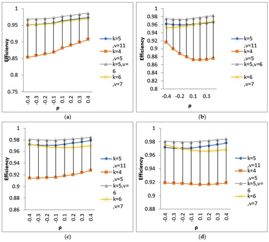
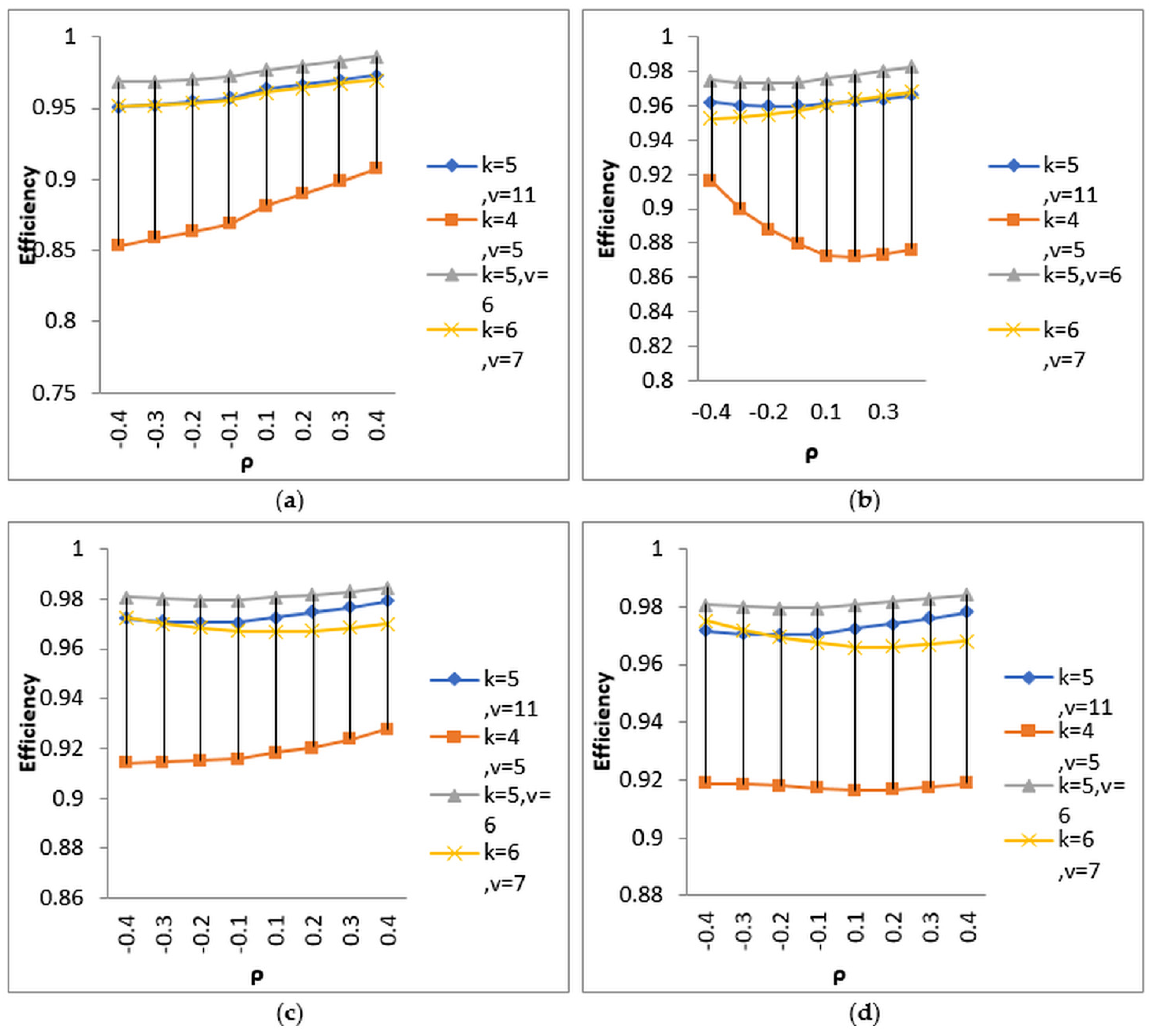
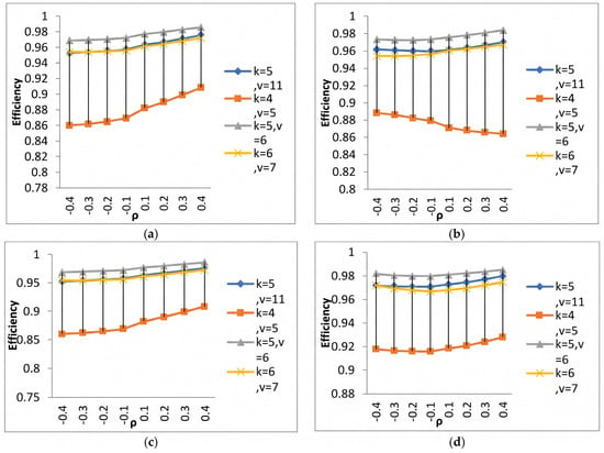
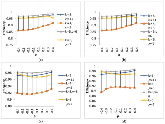
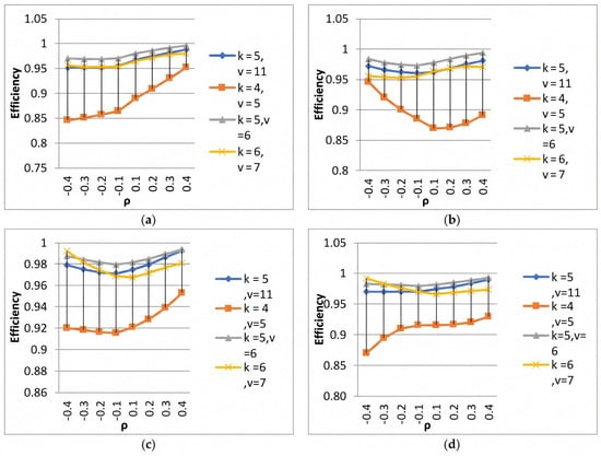
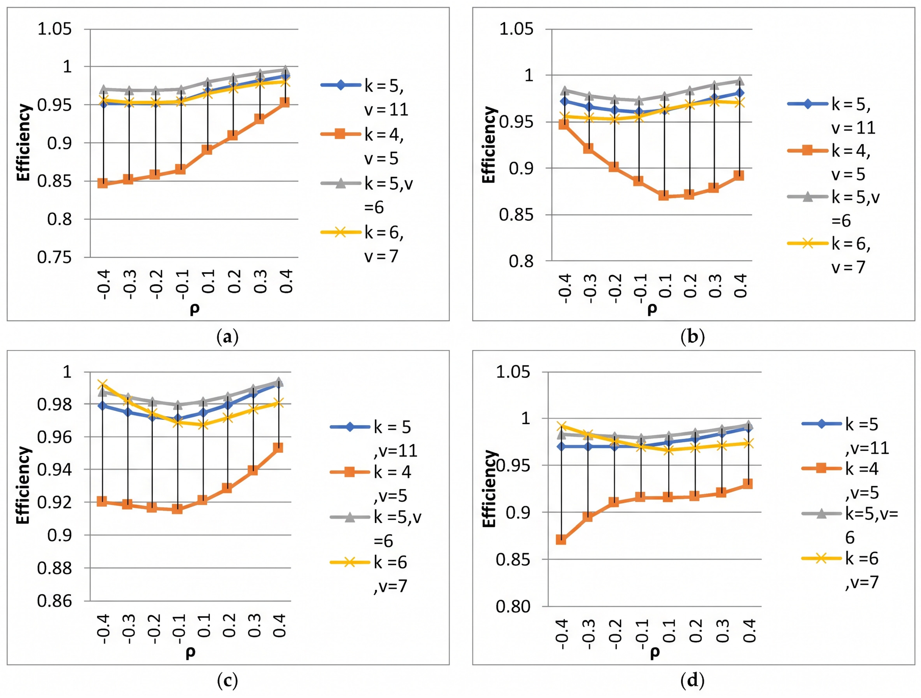
Refer to Table 1 and Figure 1a–d, which show A-efficiency and efficiency loss when one observation is missing under AR(1). In the case of the with-block-effect model, A-efficiency is continuously increasing, robustness varies within −0.4 ≤ ρ ≤ 0.4 and loss is decreasing for direct effects, but for neighbor effects, A-efficiency is decreasing, loss is increasing within −0.4 ≤ ρ ≤ −0.1 and the increase in A-efficiency and robustness is within 0.1 ≤ ρ ≤ 0.4. For the case of the without-block-effect model, A-efficiency is decreasing and loss increasing within −0.4 ≤ ρ ≤ −0.1 and there are increases in A-efficiency and decreasing loss, so for both the direct and neighbor-effects, designs are robust within 0.1 ≤ ρ ≤ 0.4.

Table 1. Relative A-efficiencies and losses due to a single missing observation, with AR(1).

Design		Relative A-Efficiency (Direct Effects)				Relative A-Efficiency (Neighbor Effects)
v	k	With Block Effect		Without Block Effect		With Block Effect		Without Block Effect
11	5	Efficiency	Loss (%)	Efficiency	Loss (%)	Efficiency	Loss (%)	Efficiency	Loss (%)
ρ
	−0.4	0.9508	4.9165	0.9720	2.8031	0.9619	3.8079	0.9715	2.8482
	−0.3	0.9525	4.7493	0.9710	2.9006	0.9604	3.9562	0.9707	2.9318
	−0.2	0.9546	4.5389	0.9706	2.9439	0.9596	4.0356	0.9704	2.9611
	−0.1	0.9571	4.2876	0.9707	2.9292	0.9595	4.0484	0.9706	2.9348
	0.1	0.9632	3.6830	0.9727	2.7301	0.9610	3.8975	0.9726	2.7350
	0.2	0.9665	3.3466	0.9745	2.5517	0.9625	3.7502	0.9742	2.5775
	0.3	0.9699	3.0055	0.9767	2.3270	0.9643	3.5707	0.9760	2.3961
	0.4	0.9732	2.6806	0.9793	2.0659	0.9662	3.3762	0.9779	2.2052
5	4
	−0.4	0.8532	14.6837	0.9139	8.6129	0.9162	8.3781	0.9188	8.1152
	−0.3	0.8583	14.1725	0.9145	8.5508	0.8996	10.0365	0.9186	8.1440
	−0.2	0.8634	13.6560	0.9150	8.4965	0.8880	11.1994	0.9179	8.2108
	−0.1	0.8689	13.1061	0.9157	8.4304	0.8801	11.9939	0.9172	8.2804
	0.1	0.8818	11.8197	0.9182	8.1848	0.8723	12.7667	0.9164	8.3559
	0.2	0.8895	11.0534	0.9204	7.9633	0.8718	12.8228	0.9167	8.3348
	0.3	0.8980	10.1980	0.9235	7.6489	0.8731	12.6854	0.9174	8.2562
	0.4	0.9074	9.2648	0.9277	7.2268	0.8763	12.3673	0.9189	8.1077
6	5
	−0.4	0.9683	3.1746	0.9809	1.9053	0.9750	2.5030	0.9808	1.9225
	−0.3	0.9690	3.1016	0.9801	1.9914	0.9735	2.6513	0.9800	2.0040
	−0.2	0.9703	2.9701	0.9797	2.0331	0.9730	2.6991	0.9796	2.0426
	−0.1	0.9721	2.7889	0.9797	2.0346	0.9734	2.6650	0.9796	2.0395
	0.1	0.9770	2.3013	0.9807	1.9315	0.9759	2.4080	0.9807	1.9300
	0.2	0.9799	2.0079	0.9817	1.8295	0.9779	2.2076	0.9817	1.8339
	0.3	0.9830	1.6954	0.9831	1.6934	0.9802	1.9756	0.9829	1.7138
	0.4	0.9862	1.3829	0.9848	1.5240	0.9827	1.7294	0.9843	1.5705
7	6
	−0.4	0.9509	4.9110	0.9728	2.7235	0.9521	4.7881	0.9751	2.4912
	−0.3	0.9522	4.7773	0.9702	2.9768	0.9534	4.6621	0.9720	2.8016
	−0.2	0.9539	4.6131	0.9684	3.1578	0.9547	4.5248	0.9696	3.0421
	−0.1	0.9559	4.4109	0.9672	3.2752	0.9564	4.3622	0.9678	3.2183
	0.1	0.9612	3.8831	0.9667	3.3332	0.9606	3.9379	0.9661	3.3869
	0.2	0.9643	3.5721	0.9673	3.2745	0.9632	3.6842	0.9662	3.3773
	0.3	0.9674	3.2576	0.9684	3.1610	0.9658	3.4240	0.9669	3.3054
	0.4	0.9702	2.9754	0.9700	3.0049	0.9681	3.1871	0.9682	3.1799

Figure 1. (a) A-efficiency for direct effects under AR(1) with block effect. (b) A-efficiency for neighbor effects under AR(1) with block effect. (c) A-efficiency for direct effects under AR(1) without block effect. (d) A-efficiency for neighbor effects under AR(1) without block effect.

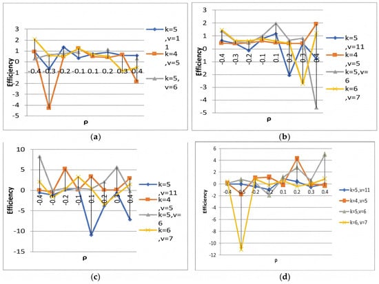
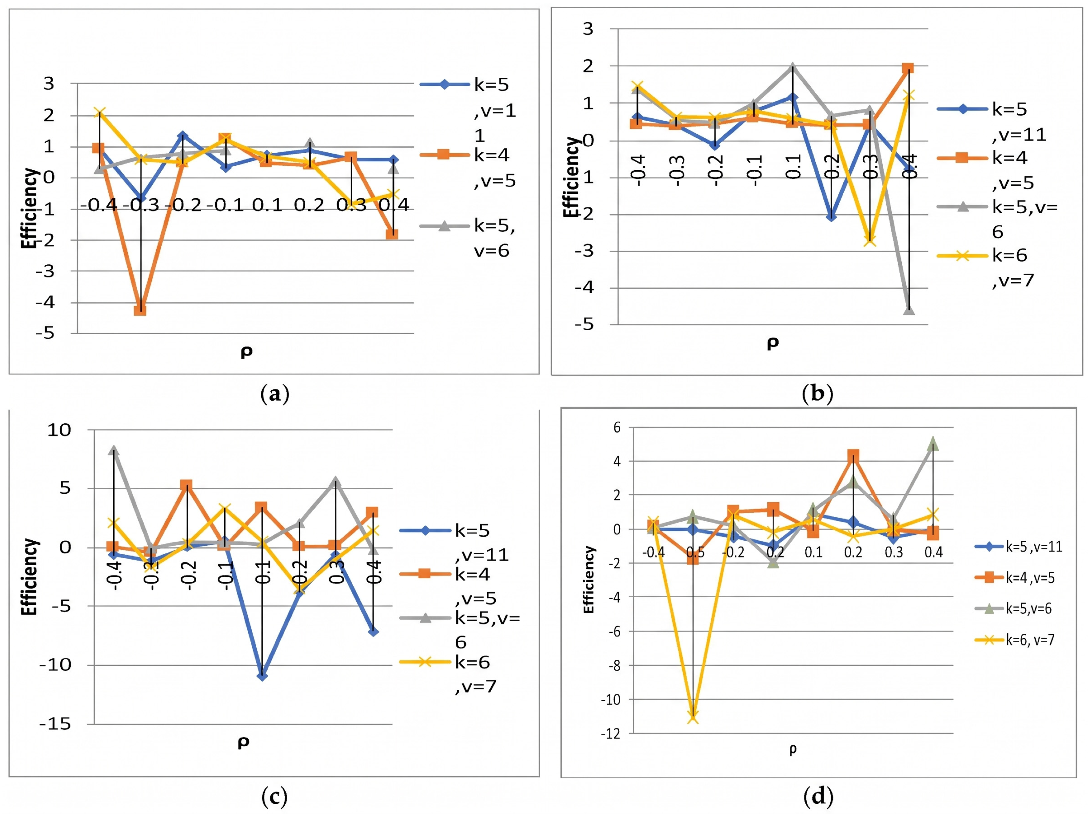
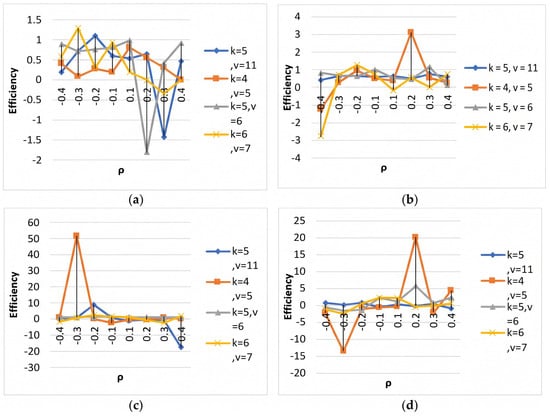
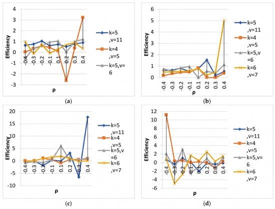
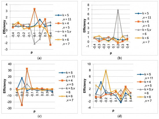
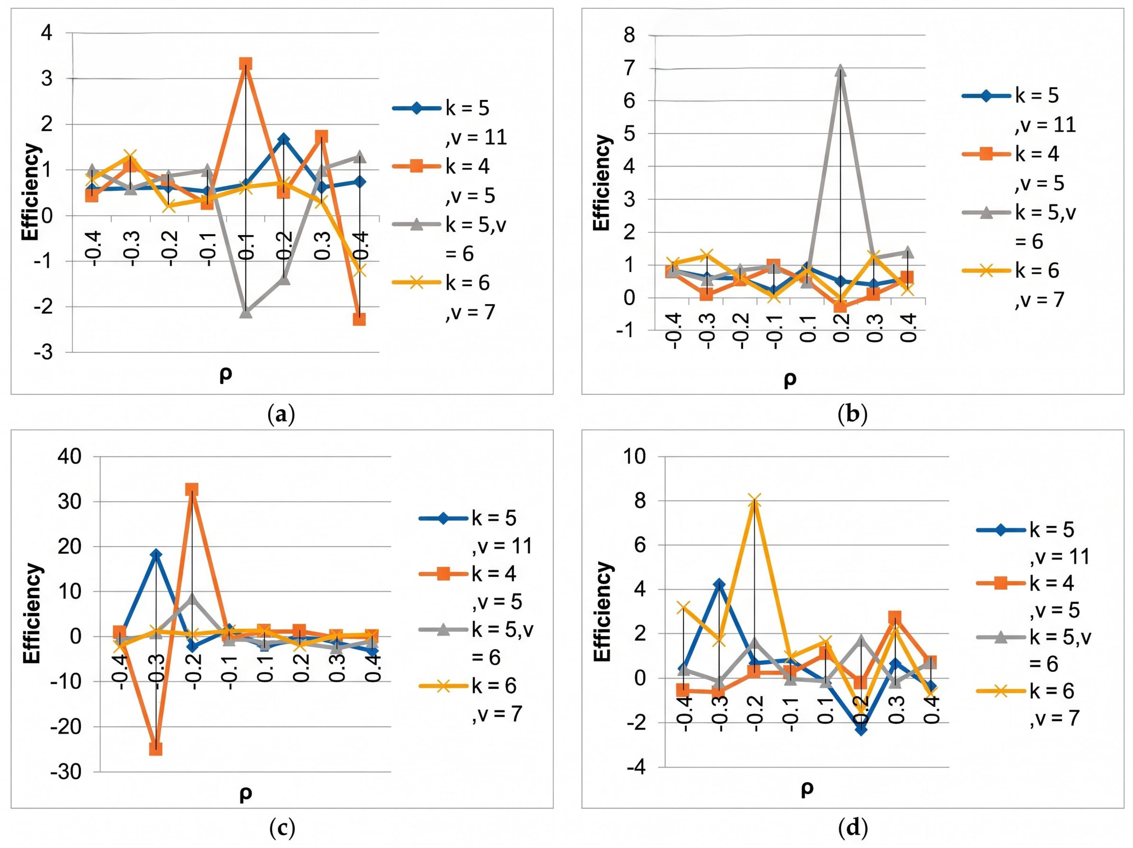
Now, refer to Table 2 and Figure 2a–d below, which present the relative D-efficiency under AR(1) when a single observation is missing A negative relative efficiency indicates that the complete design performs better than the design with one observation missing. If the relative efficiencies exceed 1.0 indicate that there is no loss of efficiency according to the specific criterion. In terms of D-efficiency, the designs demonstrate robustness across different values of ρ.

Table 2. Relative D-efficiencies and losses due to a single missing observation, with AR(1).

Design		Relative D-Efficiency (Direct Effects)				Relative D-Efficiency (Neighbor Effects)
v	k	With Block Effect		Without Block Effect		With Block Effect		Without Block Effect
11	5	Eff.	Loss (%)	Eff.	Loss (%)	Eff.	Loss (%)	Eff.	Loss (%)
ρ
	−0.4	0.9708	2.9183	−0.6040	---	0.6401	35.9949	0.0306	69.4096
	−0.3	−0.6759	----	−1.1117	---	0.4253	57.4729	−0.0602	---
	−0.2	1.3659	-----	0.0470	95.295	−0.1406	---	−0.4345	---
	−0.1	0.3465	65.3506	0.6209	37.9079	0.7965	20.3402	−0.9772	---
	0.1	0.7214	27.8631	−10.9206	---	1.1643	---	0.8834	11.6565
	0.2	0.8622	13.7793	−3.8208	---	−2.0699	---	0.3784	62.1580
	0.3	0.5686	43.1422	−0.5487	---	0.4681	53.1861	−0.4944	---
	0.4	0.5700	43.000	−7.2428	---	−0.7519	---	−0.0411	---
5	4
	−0.4	0.9162	8.3781	0.0469	95.3100	0.4375	56.2496	0.1188	95.3055
	−0.3	−4.3127	---	−0.3857	---	0.3882	61.1842	−1.6581	---
	−0.2	0.4782	52.1766	5.2550	---	0.4761	52.3887	1.0197	---
	−0.1	1.2566	---	0.0542	94.5819	0.6184	38.1564	1.1240	---
	0.1	0.4847	51.5334	3.4331	---	0.4522	54.7784	−0.0903	---
	0.2	0.3871	61.2944	0.0528	94.7242	0.4367	56.3257	4.2879	---
	0.3	0.6716	32.8440	0.1687	83.1267	0.4209	57.9081	∞	---
	0.4	−1.8303	---	2.9889	---	1.9117	---	−0.2698	---
6	5
	−0.4	0.286	71.1382	8.2232	---	1.3813	---	0.1278	87.2208
	−0.3	0.6502	34.9835	−0.0665	---	0.5875	41.2470	0.7238	27.6222
	−0.2	0.7570	24.3053	0.4946	50.5386	0.4625	53.7462	0.2009	79.9118
	−0.1	0.8762	12.3807	0.4104	58.9592	1.0055	---	−1.9074	---
	0.1	∞	∞	0.3150	68.5038	1.9779	---	1.1236	---
	0.2	1.1498	---	2.0885	---	0.6738	32.6198	2.7762	---
	0.3	∞	∞	5.6971	---	0.8384	16.1631	0.5699	43.0051
	0.4	0.2779	72.2056	−0.2314	---	−4.5940	---	4.9929	---
7	6
	−0.4	2.1077	---	2.0789	---	1.4964	---	0.3582	64.1844
	−0.3	0.6028	39.7202	−1.6760	---	0.6550	34.5046	−11.0791	---
	−0.2	0.5173	48.2725	0.3647	63.5349	0.6511	34.8938	0.8315	16.8502
	−0.1	1.2054	---	3.3257	---	0.7864	21.3620	−0.1965	---
	0.1	0.7041	29.5923	0.5694	43.0550	0.6233	37.6666	0.5855	41.4506
	0.2	0.5205	47.9541	−3.5993	---	0.4232	57.6798	−0.4258	---
	0.3	−0.8319	---	−0.9922	---	−2.7387	---	0	100
	0.4	−0.5073	---	1.4263	---	1.2476	---	0.8362	16.3841

Figure 2. (a) D-efficiency for direct effects under AR(1) with block effect, (b) D-efficiency for neighbor effects under AR(1) with block effect, (c) D-efficiency for direct effects under AR(1) without block effect, (d) D-efficiency for neighbor effects under AR(1) without block effect.

Table 3 and Figure 3a–d provide information about A-efficiency relative to a single missing observation under MA(1). In case of the with-block-effect model, A-efficiency is continuously increasing within −0.4 ≤ ρ ≤ 0.4 and loss is decreasing for direct effects, but for neighbor effects, A-efficiency is decreasing and loss is increasing within −0.4 ≤ ρ ≤ −0.1 and increasing in A-efficiency and decreasing loss within 0.1 ≤ ρ ≤ 0.4, but for v = 6, k = 5 and v = 7, k = 6. A-efficiency is increasing within −0.4 ≤ ρ ≤ 0.4.

Table 3. Relative A-efficiencies and losses due to a single missing observation, with MA(1).

Design		Relative A-Efficiency (Direct Effects)				Relative A-Efficiency (Neighbor Effects)
v	k	With Block Effect		Without Block Effect		With Block Effect		Without Block Effect
11	5	Eff.	Loss (%)	Eff.	Loss (%)	Eff.	Loss (%)	Eff.	Loss (%)
ρ
	−0.4	0.9533	4.6715	0.9717	2.8276	0.9618	3.8248	0.9680	3.1958
	−0.3	0.9541	4.5950	0.9710	2.8956	0.9608	3.9194	0.9691	3.0938
	−0.2	0.9554	4.4646	0.9707	2.9336	0.9600	3.9975	0.9698	3.0151
	−0.1	0.9573	4.2682	0.9708	2.9250	0.9597	4.0336	0.9706	2.9435
	0.1	0.9634	3.6640	0.9728	2.7245	0.9613	3.8742	0.9727	2.7342
	0.2	0.9672	3.2753	0.9747	2.5311	0.9635	3.6481	0.9744	2.5594
	0.3	0.9714	2.8594	0.9771	2.2909	0.9667	3.3344	0.9767	2.3302
	0.4	0.9755	2.4478	0.9797	2.0263	0.9703	2.9673	0.9794	2.0590
5	4
	−0.4	0.8600	14.0000	0.9176	8.2413	0.8886	11.1386	0.9027	9.7257
	−0.3	0.8620	13.8025	0.9165	8.3480	0.8858	11.4247	0.9096	9.0317
	−0.2	0.8650	13.5007	0.9159	8.4105	0.8824	11.7557	0.9141	8.5876
	−0.1	0.8693	13.0705	0.9159	8.4105	0.8788	12.1200	0.9163	8.3672
	0.1	0.8821	11.7939	0.9183	8.1709	0.8713	12.8707	0.9158	8.4248
	0.2	0.8902	10.9753	0.9207	7.9250	0.8680	13.1989	0.9143	8.5732
	0.3	0.8992	10.0822	0.9239	7.6073	0.8656	13.4449	0.9129	8.7133
	0.4	0.9084	9.1612	0.9276	7.2371	0.8643	13.5702	0.9121	8.7932
6	5
	−0.4	0.9688	3.1223	0.9818	1.8248	0.9732	2.6819	0.9797	2.0266
	−0.3	0.9694	3.0621	0.9807	1.9887	0.9729	2.7095	0.9796	2.0354
	−0.2	0.9705	2.9514	0.9800	1.9997	0.9729	2.7083	0.9796	2.0438
	−0.1	0.9722	2.7847	0.9797	2.0256	0.9734	2.6638	0.9796	2.0368
	0.1	0.9770	2.2997	0.9808	1.9235	0.9760	2.4023	0.9808	1.9230
	0.2	0.9799	2.0082	0.9820	1.8040	0.9782	2.1812	0.9820	1.8027
	0.3	0.9829	1.7118	0.9834	1.6554	0.9808	1.9151	0.9835	1.6456
	0.4	0.9857	1.4346	0.9850	1.4970	0.9837	1.6296	0.9853	1.4684
7	6
	−0.4	0.9543	4.5723	0.9717	2.8281	0.9543	4.5723	0.9745	2.5488
	−0.3	0.9542	4.5782	0.9694	3.0637	0.9545	4.5515	0.9718	2.8181
	−0.2	0.9548	4.5240	0.9676	3.2393	0.9552	4.4840	0.9694	3.0615
	−0.1	0.9561	4.3894	0.9667	3.3335	0.9564	4.3547	0.9676	3.2419
	0.1	0.9613	3.8652	0.9676	3.2373	0.9606	3.9376	0.9667	3.3268
	0.2	0.9649	3.5092	0.9694	3.0570	0.9630	3.6969	0.9677	3.2324
	0.3	0.9687	3.1304	0.9718	2.8152	0.9652	3.4780	0.9693	3.0749
	0.4	0.9724	2.7603	0.9746	2.5417	0.9669	3.3081	0.9711	2.8863

Figure 3. (a) A-efficiency for direct effects under MA(1) with block effect, (b) A-efficiency for neighbor effects under MA(1) with block effect, (c) A-efficiency for direct effects under MA(1) without block effect, (d) A-efficiency for neighbor effects under MA(1) without block effect.

In the case of the without-block-effect model, A-efficiency is decreasing and there is increasing loss within −0.4 ≤ ρ ≤ −0.1 and there are increases in A-efficiency and decreasing loss within 0.1 ≤ ρ ≤ 0.4 for both the direct and the neighbor effects.

Table 4 and Figure 4a–d provide information about D-efficiency given a single missing observation under MA(1). In the case of the with-block-effect model, D-efficiency is maximum or minimum for values of ρ, but for some values D_Rel is negative; then, the C_d complete design is better than the design with one observation missing. Relative efficiencies above 1.0 indicate that there is no loss in efficiency. Without block effects, D-efficiency varies for direct and neighbor effects.

Table 4. Relative D-efficiencies and losses due to a single missing observation, with MA(1).

Design		Relative D-Efficiency (Direct Effects)				Relative D-Efficiency (Neighbor Effects)
v	k	With Block Effect		Without Block Effect		With Block Effect		Without Block Effect
11	5	Eff.	Loss (%)	Eff.	Loss (%)	Eff.	Loss (%)	Eff.	Loss (%)
ρ
	−0.4	0.1947	80.5310	−0.1924	---	0.4026	59.7367	0.6340	36.6028
	−0.3	0.7258	27.4195	0.8817	11.8274	0.6306	36.9414	0.0572	94.2841
	−0.2	1.1060	---	8.9060	---	0.6473	35.2726	0.6633	33.6746
	−0.1	0.6015	39.8545	0.6341	36.5900	0.5926	40.7445	−0.5973	---
	0.1	0.5419	45.8138	−1.2918	---	0.6558	34.4220	0.2688	73.1209
	0.2	0.6506	34.9443	−0.0117	---	0.4977	50.2268	−0.1975	---
	0.3	−1.4261	---	−0.7855	---	0.7499	25.0134	0.4438	55.6240
	0.4	0.4763	52.3666	−17.4784	---	0.5863	41.3742	−1.0349	---
5	4
	−0.4	0.4044	59.5600	0.8304	16.9637	−1.2275	---	−2.4006	---
	−0.3	0.0778	92.2200	51.6714	---	0.2624	73.7600	−13.5058	---
	−0.2	0.2676	73.2400	−0.1772	---	0.9692	3.0800	−1.0045	---
	−0.1	0.2001	79.9900	−2.4397	---	0.5065	49.3500	−0.5868	---
	0.1	0.8085	19.1500	−0.5553	---	0.3926	60.7400	−0.5054	---
	0.2	0.5502	44.9800	−0.4441	---	3.1070	---	20.0539	---
	0.3	0.3005	69.9500	0.7457	25.4288	0.5395	46.0500	−2.1162	---
	0.4	0	100	0.1328	86.7199	0.2815	71.8500	4.4103	---
6	5
	−0.4	0.8989	10.1100	−2.0958	---	0.8091	19.0900	−0.7005	---
	−0.3	0.7059	29.41	−1.0361	---	0.6796	32.0400	−1.6565	---
	−0.2	0.7578	24.2200	∞	---	0.6427	35.7300	−1.4058	---
	−0.1	0.8180	18.2000	−0.2015	---	1.02179	---	2.2672	---
	0.1	0.9824	1.7600	12.7442	---	0.5251	---	1.0328	---
	0.2	−1.8078	---	−0.3661	---	0.4498	55.0200	5.7606	---
	0.3	0.4161	58.3900	−0.2304	---	1.1389	---	0.6530	34.7000
	0.4	0.9266	7.3400	−1.8567	---	0.1155	88.45	2.3105	---
7	6
	−0.4	0.5849	41.5100	−1.7942	---	−2.7426	---	−1.1116	---
	−0.3	1.2973	---	0.7440	25.5983	0.7079	29.21	−2.5993	---
	−0.2	0.2999	70.0100	2.5496	---	1.25328	---	0.4335	56.6530
	−0.1	0.9478	5.2200	1.4173	---	0.7438	25.6200	2.1619	---
	0.1	0.2014	79.86	0.9708	2.9153	−0.1603	---	2.2116	---
	0.2	∞	∞	−0.4937	---	0.5796	42.0400	−0.5026	---
	0.3	−0.3348	---	−2.2818	---	∞	∞	−0.1281	---
	0.4	0	100	2.1511	---	0.7378	---	0.4410	55.8993

Figure 4. (a) D-efficiency for direct effects under MA(1) with block effect, (b) D-efficiency for neighbor effects under MA(1) with block effect, (c) D-efficiency for direct effects under MA(1) without block effect, (d) D-efficiency for neighbor effects under MA(1) without block effect.

Table 5 and Figure 5a–d show relative A-efficiency given a single missing observation under NN. For the with-block-effect model, A-efficiency is continuously increasing within −0.4 ≤ ρ ≤ 0.4 and loss is decreasing for direct effects, but for neighbor effects A-efficiency is declining and loss is growing −0.4 ≤ ρ ≤ −0.1 and there are increases in A-efficiency and decreasing loss within 0.1 ≤ ρ ≤ 0.4, but for v = 5, k = 4 A-efficiency is decreasing within −0.4 ≤ ρ ≤ 0.4. For the without-block-effect model A-efficiency is decreasing and loss increasing within −0.4 ≤ ρ ≤ −0.1 and there are increases in A-efficiency and decreasing loss within 0.1 ≤ ρ ≤ 0.4 for both direct and neighbor effects, but with. v = 11, k = 5 and v = 6, k = 5, A-efficiency is increasing for neighbor effects within −0.4 ≤ ρ ≤ 0.4.

Table 5. Relative A-efficiencies and losses due to a single missing observation, with NN.

Design		Relative A-Efficiency (Direct Effects)				Relative A-Efficiency (Neighbor Effects)
v	k	With Block Effect		Without Block Effect		With Block Effect		Without Block Effect
11	5	Eff.	Loss (%)	Eff.	Loss (%)	Eff.	Loss (%)	Eff.	Loss (%)
ρ
	−0.4	0.9529	4.7093	0.9725	2.7466	0.9627	3.7323	0.9667	3.3267
	−0.3	0.9537	4.6257	0.9712	2.8754	0.9611	3.8887	0.9688	3.1247
	−0.2	0.9552	4.4785	0.9707	2.9319	0.9601	3.9920	0.9698	3.0213
	−0.1	0.9573	4.2706	0.9707	2.9254	0.9597	4.0336	0.9706	2.9255
	0.1	0.9634	3.6602	0.9728	2.7228	0.9613	3.8724	0.9727	2.7327
	0.2	0.9676	3.2397	0.9749	2.5118	0.9638	3.6239	0.9746	2.5416
	0.3	0.9728	2.7201	0.9780	2.2042	0.9678	3.2158	0.9776	2.2435
	0.4	0.9792	2.0717	0.9824	1.7639	0.9740	2.5937	0.9823	1.7738
5	4
	−0.4	0.8588	14.1182	0.9189	8.1101	0.8910	10.9039	0.8939	10.6137
	−0.3	0.8612	13.8784	0.9168	8.3164	0.8868	11.3240	0.9076	9.2409
	−0.2	0.8647	13.5318	0.9159	0.4073	0.8827	11.7254	0.9138	0.6172
	−0.1	0.8692	13.0756	0.9159	8.4109	0.8788	12.1162	0.9163	8.3684
	0.1	0.8821	11.7861	0.9183	8.1608	0.8713	12.8743	0.9157	8.4261
	0.2	0.8910	10.8998	0.9210	7.8999	0.8678	13.2241	0.9141	8.5866
	0.3	0.9022	9.7758	0.9251	7.4886	0.8650	13.5018	0.9125	8.7486
	0.4	0.9174	8.2623	0.9316	6.8388	0.8645	13.5501	0.9122	8.7844
6	5
	−0.4	0.9686	3.1435	0.9830	1.7028	0.9736	2.6393	0.9797	2.0291
	−0.3	0.9691	3.0873	0.9810	1.8970	0.9730	2.7028	0.9797	2.0319
	−0.2	0.9704	2.9632	0.9800	1.9951	0.9729	2.7099	0.9796	2.0434
	−0.1	0.9721	2.7867	0.9797	2.0256	0.9734	2.6646	0.9796	2.0370
	0.1	0.9770	2.2968	0.9808	1.9226	0.9760	2.4004	0.9808	1.9220
	0.2	0.9802	1.9822	0.9821	1.7920	0.9784	2.1595	0.9821	1.7903
	0.3	0.9838	1.6161	0.9840	1.6026	0.9818	1.8206	0.9841	1.5878
	0.4	0.9880	1.1986	0.9865	1.3509	0.9864	1.3561	0.9871	1.2941
7	6
	−0.4	0.9547	4.5317	0.9781	2.1895	0.9545	4.5482	0.9782	2.1794
	−0.3	0.9542	4.5817	0.9728	2.7163	0.9544	4.5617	0.9738	2.6214
	−0.2	0.9547	4.5317	0.9695	3.0510	0.9551	4.4923	0.9703	2.9678
	−0.1	0.9561	4.3912	0.9675	3.2499	0.9564	4.3564	0.9680	3.2017
	0.1	0.9614	3.8618	0.9669	3.3095	0.9606	3.9351	0.9663	3.3748
	0.2	0.9652	3.4766	0.9682	3.1794	0.9632	3.6765	0.9666	3.3377
	0.3	0.9700	3.0047	0.9706	2.9366	0.9659	3.4149	0.9677	3.2346
	0.4	0.9547	4.5317	0.9744	2.5600	0.9545	4.5482	0.9692	3.0821

Figure 5. (a) A-efficiency for direct effects under NN with block effect, (b) A-efficiency for neighbor effects under NN with block effect, (c) A-efficiency for direct effects under NN without block effect, (d) A-efficiency for neighbor effects under NN without block effect.

Table 6 and Figure 6a–d show D-efficiency relative to a single missing observation under NN. In the case of the with-block-effects model, relative D-efficiency varies across the correlation values. A negative value indicates that the complete design performs better than the design with one missing observation; values above 1.0 indicate no efficiency loss. For the without-block-effect model, D-efficiency varies irregularly across ρ for both direct and neighbor effects.

Table 6. Relative D-efficiencies and losses due to a single missing observation, with NN.

Design		Relative D-Efficiency (Direct Effects)				Relative D-Efficiency (Neighbor Effects)
v	k	With Block Effect		Without Block Effect		With Block Effect		Without Block Effect
11	5	Eff.	Loss (%)	Eff.	Loss (%)	Eff.	Loss (%)	Eff.	Loss (%)
ρ
	−0.4	0.6384	36.1612	−0.9237	---	0.6362	36.3807	0.7087	29.1332
	−0.3	0.7741	22.5885	−0.0045	---	0.6684	33.1625	−0.3588	---
	−0.2	1.0290	---	−1.7943	---	0.8445	15.5446	0.9945	0.0055
	−0.1	0.6221	37.7893	0.2563	74.3700	0.5118	48.8236	0.1106	88.9400
	0.1	0.7227	27.7325	∞		0.7988	20.1160	−2.0789	---
	0.2	0.5291	47.0933	3.1744	---	1.5534	---	−0.1918	---
	0.3	0.7606	23.9374	−6.5108	---	0.1894	81.0580	−0.3461	---
	0.4	0.8896	11.0443	17.7576	---	0.5528	44.7200	−0.1585	---
5	4
	−0.4	∞	---	0.0834	91.6622	0.1902	80.9800	11.1256	---
	−0.3	0.3394	0.6606	0.0846	91.5352	0.3459	65.4100	0.3361	66.3940
	−0.2	0.5930	40.7000	1.0977	---	0.4607	53.9300	0.4280	57.2042
	−0.1	0.4295	57.0500	0.3764	62.3594	0.4802	51.9800	−0.0253	---
	0.1	0.1078	89.2200	−0.9093	---	0.8375	16.2500	0.2209	77.9107
	0.2	−2.6462	---	0.7182	28.1819	0	100	−0.0762	---
	0.3	0.3750	62.5	0.5059	49.4101	∞	−−	−1.2149	---
	0.4	3.2045	---	0.8499	15.0087	0.3876	61.24	0.2130	78.7002
6	5
	−0.4	−0.5789	---	−0.5649	---	0.7798	22.0200	1.9566	---
	−0.3	0.4052	59.48	−0.3197	---	0.5689	43.1100	−1.3593	---
	−0.2	0.5808	41.9200	−0.6715	---	0.8481	15.1900	3.0867	---
	−0.1	0.9390	6.1000	0.5440	45.5959	0.9715	2.8500	−2.3557	---
	0.1	1.0420	---	6.2206	---	0	100	−0.8685	---
	0.2	0	100	0	100	0.5884	41.1600	0.95430	---
	0.3	0.9959	0.4100	0.5912	40.8823	0.3661	63.39	−1.4333	---
	0.4	1.1915	---	1.2225	---	1.1520	---	1.1923	---
7	6
	−0.4	1.0002	---	−0.3024	---	0.4879	51.2100	0.8218	17.8250
	−0.3	−0.1298	---	0.2095	79.0481	0.5294	47.0600	−4.9075	---
	−0.2	0.7085	29.15	0.9681	3.1837	0.5358	46.4200	−2.7499	---
	−0.1	−0.0713	---	1.5759	---	0.5901	40.9900	1.6434	---
	0.1	0.2685	73.1500	1.8514	---	0.8017	19.8300	0.4315	56.8462
	0.2	0.7044	29.5600	1.1127	---	0.2031	---	2.4874	---
	0.3	0.8846	11.5400	−0.1689	---	0.5318	---	0.2782	72.1819
	0.4	0.3476	65.2400	0	100	5.0252	---	1.4972	---

Figure 6. (a) D-efficiency for direct effects under NN with block effect, (b) D-efficiency for neighbor effects under NN with block effect, (c) D-efficiency for direct effects under NN without block effect, (d) D-efficiency for neighbor effects under NN without block effect.

Table 7 and Figure 7a–d show relative A-efficiency after one observation is missing under ARMA(1,1). With block effects, direct-effect A-efficiency increases, and its loss decreases for direct effects, but for v = 6, k = 5 of direct effects and for all cases, A-efficiency is declining and loss is growing −0.4 ≤ ρ ≤ −0.1 and there are increases in A-efficiency and decreasing loss within 0.1 ≤ ρ ≤ 0.4. For the without-block-effect model, A-efficiency is decreasing and there is increasing loss within −0.4 ≤ ρ ≤ −0.1 and increasing A-efficiency and decreasing loss within 0.1 ≤ ρ ≤ 0.4 for both direct and neighbor effects, but with v = 5, k = 4 and v = 7, k = 6, A-efficiency is increasing and reducing, respectively, for neighbor effects within −0.4 ≤ ρ ≤ 0.4.

Table 7. Relative A-efficiencies and losses due to a single missing observation, with ARMA(1,1).

Design		Relative A-Efficiency (Direct Effects)				Relative A-Efficiency (Neighbor Effects)
v	k	With Block Effect		Without Block Effect		With Block Effect		Without Block Effect
11	5	Eff.	Loss (%)	Eff.	Loss (%)	Eff.	Loss (%)	Eff.	Loss (%)
ρ
	−0.4	0.9520	4.7961	0.9789	2.1107	0.9717	2.8330	0.9706	2.9404
	−0.3	0.9513	4.8686	0.9752	2.4821	0.9664	3.3600	0.9706	2.4821
	−0.2	0.9521	4.7857	0.9721	2.7913	0.9623	3.7749	0.9701	2.9874
	−0.1	0.9550	4.5023	0.9706	2.9367	0.9599	4.0113	0.9702	2.9813
	0.1	0.9669	3.3062	0.9746	2.5403	0.9630	3.6999	0.9743	2.5705
	0.2	0.9749	2.5107	0.9798	2.0217	0.9685	3.1458	0.9788	2.1208
	0.3	0.9824	1.7594	0.9861	1.3887	0.9753	2.4713	0.9844	1.5560
	0.4	0.9879	1.2130	0.9923	0.7717	0.9813	1.8705	0.9902	0.9783
5	4
	−0.4	0.8460	15.3961	0.9199	8.0110	0.9457	5.4309	0.8694	13.0566
	−0.3	0.8511	14.8891	0.9180	8.2028	0.9196	8.0396	0.8945	10.5542
	−0.2	0.8567	14.3317	0.9162	08.3827	0.8997	10.0286	0.9095	9.0492
	−0.1	0.8642	13.5809	0.9155	8.4507	0.8850	11.5007	0.9159	8.4119
	0.1	0.8900	11.0000	0.9206	7.9416	0.8700	13.0000	0.9155	8.4469
	0.2	0.9089	9.1121	0.9280	7.1987	0.8707	12.9261	0.9160	8.4030
	0.3	0.9303	6.9690	0.9390	6.0987	0.8779	12.2121	0.9204	7.9592
	0.4	0.9518	4.8234	0.9528	4.7172	0.8908	10.9165	0.9296	7.0445
6	5
	−0.4	0.9711	2.8903	0.9876	1.2399	0.9839	1.6130	0.9828	1.7236
	−0.3	0.9687	3.1328	0.9842	1.5832	0.9778	2.2190	0.9819	1.8111
	−0.2	0.9684	3.1581	0.9813	1.8672	0.9741	2.5875	0.9804	1.9577
	−0.1	0.9704	2.9630	0.9798	2.0172	0.9730	2.7024	0.9796	2.0412
	0.1	0.9800	2.0000	0.9819	1.8146	0.9780	2.1935	0.9818	1.8184
	0.2	0.9864	1.3607	0.9851	1.4862	0.9835	1.6536	0.9849	1.5063
	0.3	0.9924	0.7603	0.9894	1.0626	0.9893	1.0657	0.9890	1.0960
	0.4	0.9966	0.3390	0.9940	0.6025	0.9942	0.5849	0.9936	0.6378
7	6
	−0.4	0.9558	4.4239	0.9920	0.7967	0.9552	4.4779	0.9919	0.8100
	−0.3	0.9536	4.6372	0.9819	1.8058	0.9537	4.6344	0.9833	1.6700
	−0.2	0.9529	4.7102	0.9741	2.5936	0.9534	4.6584	0.9756	2.4400
	−0.1	0.9543	4.5682	0.9689	3.1140	0.9549	4.5064	0.9698	3.6168
	0.1	0.9647	3.5340	0.9677	3.2281	0.9632	3.6822	0.9665	3.3500
	0.2	0.9720	2.8036	0.9716	2.8381	0.9682	3.1793	0.9687	3.1300
	0.3	0.9781	2.1935	0.9768	2.3193	0.9714	2.8591	0.9719	2.8100
	0.4	0.9808	1.9151	0.9810	1.9048	0.9709	2.9116	0.9737	2.6300

Figure 7. (a) A-efficiency for direct effects under ARMA(1,1) with block effect, (b) A-efficiency for neighbor effects under ARMA(1,1) with block effect, (c) A-efficiency for direct effects under ARMA(1,1) without block effect, (d) A-efficiency for neighbor effects under ARMA(1,1) without block effect.

The results given in Table 8 and Figure 8a–d offer information about D-efficiency given a single missing observation under ARMA(1,1). In the case of the with-block-effect model, relative D-efficiency is extreme or smallest for some values of ρ but for some values D_Rel is negative, indicating that the complete design is better than the condensed design. Relative efficiencies that are surpassing 1.0 show no loss in efficiency. For the without-block-effect model, D-efficiency with ARMA(1,1) has arbitrary drift for values of ρ for direct and neighbor effects.

Table 8. Relative D-efficiencies and losses due to single missing observation, with ARMA(1,1).

Design		Relative D-Efficiency (Direct Effects)				Relative D-Efficiency (Neighbor Effects)
v	k	With Block Effect		Without Block Effect		With Block Effect		Without Block Effect
11	5	Eff.	Loss (%)	Eff.	Loss (%)	Eff.	Loss (%)	Eff.	Loss (%)
ρ
	−0.4	0.6019	39.8061	−0.4788	---	0.8370	16.3046	0.4540	54.5963
	−0.3	0.5995	40.0521	18.2388	---	0.6327	36.7287	4.2390	---
	−0.2	0.6102	38.9838	−2.5160	---	0.5682	43.1784	0.6732	32.6770
	−0.1	0.5430	45.6979	1.6229	---	0.2198	78.0186	0.8593	14.0726
	0.1	0.6674	33.2606	−2.3401	---	0.8841	11.5894	−0.1816	---
	0.2	1.6772	---	−0.1980	---	0.4916	50.8386	−2.3057	---
	0.3	0.6168	38.3182	−1.4029	---	0.4272	57.2793	0.6668	33.3214
	0.4	0.7512	24.8759	−3.4842	---	0.5750	42.5018	−0.3628	---
5	4
	−0.4	0.4014	59.86	0.8633	31.6651	0.7329	26.7100	−0.5656	---
	−0.3	1.0600	---	−25.2656	---	0.0706	92.9400	−0.5857	---
	−0.2	0.7332	26.6800	32.2079	---	0.4788	52.1200	0.2356	76.4418
	−0.1	0.2266	77.3400	−0.0877	---	0.9263	7.3700	0.2538	74.6190
	0.1	3.2962	---	1.1197	---	0.5471	45.2900	1.0515	---
	0.2	0.4611	53.8900	0.9651	3.5487	−0.3131	---	−0.1991	---
	0.3	1.7050	---	−0.2189	---	0.0683	93.1700	2.6737	---
	0.4	−2.3118	---	−0.1968	---	0.5744	42.5600	0.6404	35.9594
6	5
	−0.4	1.0009	---	−0.8530	---	0.8254	17.4600	0.3687	63.1346
	−0.3	0.5813	41.8700	0.3938	60.6245	0.5298	47.0200	−0.0955	---
	−0.2	0.8667	13.3300	8.2367	---	0.8638	13.6200	1.6140	---
	−0.1	0.9953	0.47	−0.8531	---	0.8996	10.0400	−0.0298	---
	0.1	−2.1090	---	−1.4226	---	0.4495	55.0500	−0.0988	---
	0.2	−1.3932	---	−1.2472	---	6.9181	---	1.7383	---
	0.3	1.0016	---	−2.7064	---	1.1861	---	−0.1892	---
	0.4	1.2977	---	−0.9698	---	1.3879	---	0.7695	23.0499
7	6
	−0.4	0.7931	20.6900	−2.1729	---	1.0065	---	3.1409	---
	−0.3	1.3000	---	1.2073	---	1.2724	---	1.7243	---
	−0.2	0.1935	80.6500	0.4832	51.6765	0.6267	37.3300	8.0838	---
	−0.1	0.3889	61.1100	1.2980	---	0.0460	95.4000	0.9638	3.6168
	0.1	0.6146	38.5400	1.2362	---	0.8116	18.8400	1.6927	---
	0.2	0.7245	27.5500	−1.7590	---	0	100	−1.3993	---
	0.3	0.2945	70.5500	0.3013	69.8698	1.2188	---	2.1204	---
	0.4	−1.2041	---	0.3744	62.5570	0.2458	75.4200	−0.7601	---

Figure 8. (a) D-efficiency for direct effects under ARMA(1,1) with block effect, (b) D-efficiency for neighbor effects under ARMA(1,1) with block effect, (c) D-efficiency for direct effects under ARMA(1,1) without block effect, (d) D-efficiency for neighbor effects under ARMA(1,1) without block effect.

Furthermore, Table 9 and Table 10 summarize optimal A-efficiency with loss (%) for direct and neighbor effects respectively, with block effect and without block effect, and under different correlated structures. For direct effects, for the with-block-effect model, in almost all structures, A-efficiency is optimal at ρ = 0.4; for neighbor effects it is optimal for other reported values. In the without-block-effect model, for direct effects, in almost all structures, A-efficiency has an optimal value at ρ = 0.4 except v = 7, k = 6 but for neighbor effects it is optimal at |ρ| = 0.4 and at ρ = −0.1. Here efficiency shows the robustness of a design with a missing observation at different values of ρ under different correlated structures.

Table 9. Optimal relative A-efficiency and loss for direct effects, with block effect and without block effect, under correlated structures.

Structure	Design		With-Block-Effect Model			Without-Block-Effect Model
AR(1)	v	k	ρ	A-efficiency	Loss (%)	ρ	A-efficiency	Loss (%)
	11	5	0.4	0.9732	2.6806	0.4	0.9793	2.0659
	5	4	0.4	0.9074	9.2648	0.4	0.9277	7.2268
	7	6	0.4	0.9862	1.3829	0.4	0.9848	1.5240
	6	5	0.4	0.9702	2.9754	-0.4	0.9728	2.7235
MA(1)	11	5	0.4	0.9755	2.4478	0.4	0.9797	2.0263
	5	4	0.4	0.9084	9.1612	0.4	0.9276	7.2371
	7	6	0.4	0.9857	1.4346	0.4	0.9850	1.4970
	6	5	0.4	0.9724	2.7603	0.4	0.9746	2.5417
NN	11	5	0.4	0.9792	2.0717	0.4	0.9824	1.7639
	5	4	0.4	0.9174	8.2623	0.4	0.9316	6.8388
	7	6	0.4	0.9880	1.1986	0.4	0.9865	1.3509
	6	5	0.3	0.9700	3.0047	-0.4	0.9781	2.1895
ARMA(1,1)	11	5	0.4	0.9879	1.2130	0.4	0.9923	0.7717
	5	4	0.4	0.9518	4.8234	0.4	0.9528	4.7172
	7	6	0.4	0.9966	0.3390	0.4	0.9940	0.6025
	6	5	0.4	0.9808	1.9151	-0.4	0.9920	0.7967

Table 10. Optimal relative A-efficiency and loss for neighbor effects with block effect under correlated structures.

Structure	Design		With-Block-Effect Model			Without-Block-Effect Model
AR(1)	v	k	ρ	A-efficiency	Loss (%)	ρ	A-efficiency	Loss (%)
	11	5	−0.1	0.7965	20.3402	0.4	0.9779	2.0252
	5	4	−0.1	0.6184	38.1564	0.4	0.9189	8.1077
	7	6	0.3	0.8384	16.1631	0.4	0.9843	1.5705
	6	5	−0.1	0.7864	21.3620	−0.4	0.9751	2.4912
MA(1)	11	5	0.3	0.7499	25.0134	0.4	0.9794	2.0590
	5	4	−0.2	0.9692	3.0800	0.4	0.9121	8.7932
	7	6	−0.4	0.8091	19.0900	0.4	0.9853	1.4684
	6	5	−0.1	0.7438	25.6200	−0.4	0.9745	2.5488
NN	11	5	−0.2	0.8445	15.5446	0.4	0.9823	1.7738
	5	4	0.1	0.8375	16.2500	−0.1	0.9163	8.3684
	7	6	−0.1	0.9715	2.8500	0.4	0.9871	1.2941
	6	5	0.1	0.8017	19.8300	−0.4	0.9782	2.1794
ARMA(1,1)	11	5	−0.4	0.8370	16.3046	0.4	0.9902	0.9783
	5	4	−0.1	0.9263	7.3700	0.4	0.9296	7.0445
	7	6	−0.1	0.8996	10.0400	0.4	0.9936	0.6378
	6	5	0.1	0.8116	18.8400	−0.4	0.9919	0.8072

Table 11 and Table 12 present optimal relative D-efficiencies and loss for the with-block-effect and the without-block-effect models for direct and neighbor effects, respectively. Under both models, D-efficiency for direct and neighbor effects varies irregularly across ρ under all correlated structures. As optimality criteria summarize how good a design is, here, optimal values provide information describing for what value of ρ a design is optimal. Such optimality criteria function as a précis of how good a design is; here, efficiency offers evidence for the value of ρ at which a design is optimal.

Table 11. Optimal relative D-efficiency and loss for direct effects, with block effect and without block effect, under correlated structures.

Structure	Design		With-Block-Effect Model			Without-Block-Effect Model
AR(1)	v	k	ρ	D-efficiency	Loss (%)	ρ	D-efficiency	Loss (%)
	11	5	−0.4	0.9708	2.9183	−0.1	0.6209	37.9079
	5	4	−0.4	0.9162	8.3781	0.3	0.1687	83.1267
	7	6	−0.1	0.8762	12.3807	−0.2	0.4946	50.538
	6	5	0.1	0.7041	29.5923	0.1	0.5694	43.0550
MA(1)	11	5	−0.3	0.7258	27.4195	−0.3	0.8817	11.8274
	5	4	0.1	0.8085	19.1500	−0.4	0.8304	16.9637
	7	6	0.1	0.9824	1.7600	---	---	---
	6	5	−0.1	0.9478	5.2200	0.1	0.9708	2.9153
NN	11	5	0.4	0.8896	11.0443	−0.1	0.2563	74.3700
	5	4	−0.2	0.5930	40.7000	0.4	0.8499	15.0087
	7	6	0.3	0.9959	0.4100	0.3	0.5912	40.8823
	6	5	0.3	0.8846	11.5400	−0.2	0.9681	3.1837
ARMA(1,1)	11	5	0.4	0.7512	24.8759	---	---	---
	5	4	−0.2	0.7332	26.6800	0.2	0.9651	3.5487
	7	6	−0.1	0.9953	0.4700	−0.3	0.3938	60.6245
	6	5	−0.4	0.7931	20.6900	−0.2	0.4832	51.6765

Table 12. Optimal relative D-efficiency and loss for neighbor effects, with block effect and without block effect, under correlated structures.

Structure	Design		With-Block-Effect Model			Without-Block-Effect Model
AR(1)	v	k	ρ	D-efficiency	Loss (%)	ρ	D-efficiency	Loss (%)
	11	5	−0.1	0.7965	20.3402	0.1	0.8834	11.6565
	5	4	−0.1	0.6184	38.1564	−0.4	0.1188	95.3055
	7	6	0.3	0.8384	16.1631	−0.3	0.7238	27.6222
	6	5	−0.1	0.7864	21.3620	0.4	0.8362	16.3841
MA(1)	11	5	0.3	0.7499	25.0134	−0.2	0.6633	33.6746
	5	4	−0.2	0.9692	3.0800	---	---	---
	7	6	−0.4	0.8091	19.0900	0.3	0.6530	34.7000
	6	5	−0.1	0.7438	25.6200	0.4	0.4410	55.8993
NN	11	5	−0.2	0.8445	15.5446	−0.4	0.7087	29.1332
	5	4	0.1	0.8375	16.2500	−0.2	0.4280	57.2042
	7	6	−0.1	0.9715	2.8500	---	---	---
	6	5	0.1	0.8017	19.8300	−0.4	0.8218	17.8250
ARMA(1,1)	11	5	−0.4	0.8370	16.3046	−0.1	0.8593	14.0726
	5	4	−0.1	0.9263	7.3700	0.4	0.6404	35.9594
	7	6	−0.1	0.8996	10.0400	0.4	0.7695	23.0499
	6	5	0.1	0.8116	18.8400	−0.1	0.9638	3.6168

6. Concluding Remarks

This study reviews the sufficient conditions for the universal optimality of CNBDs given by [24]. It considers the models and information matrices for the cases b = v = 2k + 1 and v = k + 1 for v treatments and n experimental units, with direct and neighbor effects. The study also considers designs with v = k + 1 treatments compared with v treatments and n experimental units. We discuss the universal optimality of these design classes and assess their robustness when a single observation is missing under different correlation structures, using A- and D-efficiency. The results show high A-efficiency and small losses under ARMA(1,1) for direct and neighbor effects. For direct effects, D-efficiency is high and losses are small under MA(1); for neighbor effects, ARMA(1,1) provides higher efficiency with a small loss. Overall, a missing observation has a limited effect under ARMA(1,1). Under both models, direct treatment effects are more efficient than neighbor effects.

References

- Box, G.E.P. Multifactor Designs of First Order. Biometrika 1952, 39, 49–57. [Google Scholar] [CrossRef] [Scilit]
- Mahoney, M.W. Randomized algorithms for matrices and data. Found. Trends® Mach. Learn. 2011, 3, 123–224. [Google Scholar] [CrossRef] [Scilit]
- Rees, D.H. Some designs of use in serology. Biometrics 1967, 23, 779–791. [Google Scholar] [CrossRef] [Scilit] [PubMed]
- Azais, J.M. Design of experiments for studying intergenotypic competition. J. R. Stat. Soc. Ser. B 1987, 49, 334–345. [Google Scholar] [CrossRef] [Scilit]
- Tomar, J.S.; Jaggi, S.; Varghese, C. On totally balanced block designs for competition effects. J. Appl. Stat. 2005, 32, 87–97. [Google Scholar] [CrossRef] [Scilit]
- Jaggi, S.; Kumar, D.P.; Varghese, C.; Varghese, E.; Bhowmik, A. A Note on Circular Neighbor Balanced Designs. Commun. Stat.-Simul. Comput. 2017, 47, 2896–2905. [Google Scholar] [CrossRef] [Scilit]
- Khalid, A.; Shehzad, F.; Ali, A.; Ahmed, R. Some important classes of neighbor balanced designs in linear blocks of small sizes. J. King Saud Univ.-Sci. 2018, 30, 311–315. [Google Scholar] [CrossRef] [Scilit]
- Nadeem, M.; Rasheed, M.; Tahir, M.H.; Khadija, N.; Sajid, H.; Ahmed, R. An easy construction of generalized neighbor designs in minimal circular blocks. Kuwait J. Sci. 2022, 49, 1–11. [Google Scholar] [CrossRef] [Scilit]
- Noreen, K.; Rashid, M.S.; Shehzad, F.; Ul Hassan, Z.; Noreen, Z.; Omer, T.; Ahmed, R. Algorithms to obtain generalized neighbor designs in minimal circular blocks. Commun. Stat.-Simul. Comput. 2024, 53, 3094–3105. [Google Scholar] [CrossRef] [Scilit]
- Bhowmik, A.; Jaggi, S.; Varghese, C.; Varghese, E. Universally optimal second order neighbor designs. Model Assist. Stat. Appl. 2013, 8, 309–314. [Google Scholar] [CrossRef] [Scilit]
- Jeevitha, M.; Santharam, C. Universal optimality of circular neighbor balanced design under equal right and left neighbor effects. IOSR J. Math. 2015, 11, 68–72. [Google Scholar]
- Filipiak, K.; Khodsiani, R.; Markiewicz, A. Optimality of block designs under the model with the first-order circular autoregression. Stat. Pap. 2019, 60, 427–447. [Google Scholar] [CrossRef] [Scilit]
- Kong, X.; Zhang, X.; Zheng, W. Circular designs for total effects under interference models. J. Stat. Plan. Inference 2023, 227, 146–161. [Google Scholar] [CrossRef] [Scilit]
- Khodsiani, R.; Pooladsaz, S. Optimality of circular equineighbored block designs under correlated observations. Stat. Pap. 2022, 63, 1743–1755. [Google Scholar] [CrossRef] [Scilit]
- Abeynayakea, N.; Jaggi, R.S.; Varghese, C. Robustness of neighbor blanced complete block designs against missing observation(s). Model Assist. Stat. Appl. 2011, 6, 81–87. [Google Scholar] [CrossRef] [Scilit]
- Santharam, C.; Ponnuswamy, K.N. Universal optimality of nearest neighbor balanced block designs using ARMA models. Statistica 1995, 55, 229–238. [Google Scholar]
- Tomar, J.S.; Jaggi, S. Efficient neighbor balanced block designs for correlated observations. Metron-Int. J. Stat. 2007, 65, 229–238. [Google Scholar]
- Iqbal, I.; Tahir, M.H.; Ghazali, S.S.A. Circular neighbor-balanced designs using cyclic shifts. Sci. China Ser. A Math. 2009, 52, 2243–2256. [Google Scholar] [CrossRef] [Scilit]
- Bhatti, M.I. Cluster Effects in Mining Complex Data; Nova Science: Hauppauge, NY, USA, 2012; pp. 1–265. [Google Scholar]
- Santharam, C.; Ponnusamy, K.N.; Chandrasekar, B. Universal optimality of nearest neighbor balanced block designs using second order correlated. Biom. J. 1996, 38, 725–730. [Google Scholar] [CrossRef] [Scilit]
- Raja, B.R.; Santharam, C.; Kumar, R.S. MV-Optimality of Nearest Neighbor Balanced Block Designs Using first order and Second Order Correlated Models. Int. J. Stat. Math. 2012, 2, 61–64. [Google Scholar]
- Bhatti, M.I. Optimal testing for equicorrelated linear regression models. Stat. Pap. 1995, 36, 299–312. [Google Scholar] [CrossRef] [Scilit]
- Bhatti, M.I. On optimal testing for the equality of equicorrelation: An example of loss in power. Stat. Pap. 2000, 41, 345–352. [Google Scholar] [CrossRef] [Scilit]
- Kiefer, J. Construction and optimality of generalized youden designs. In A Survey of Statistical Designs and Linear Models; Srivastava, J.N., Ed.; North Holland: Amsterdam, The Netherlands, 1975; pp. 333–353. [Google Scholar]
- Henderson, H.V. C85. On the inverse of a completely symmetric matrix. J. Stat. Comput. Simul. 1981, 12, 138–139. [Google Scholar] [CrossRef] [Scilit]
- Iqbal, I.; Tahir, M.H. Circular strongly balanced repeated measurements designs. Commun. Stat.-Theory Methods 2009, 38, 3686–3696. [Google Scholar] [CrossRef] [Scilit]
- Iwundu, M. Missing observations: The loss in relative A-, D- and G-efficiency. Int. J. Adv. Math. Sci. 2017, 5, 43–49. [Google Scholar] [CrossRef] [Scilit]
Disclaimer/Publisher’s Note: The statements, opinions and data contained in all publications are solely those of the individual author(s) and contributor(s) and not of MDPI and/or the editor(s). MDPI and/or the editor(s) disclaim responsibility for any injury to people or property resulting from any ideas, methods, instructions or products referred to in the content. |
© 2026 by the authors. Licensee MDPI, Basel, Switzerland. This article is an open access article distributed under the terms and conditions of the Creative Commons Attribution (CC BY) license.