


Abstract
Highway–rail grade crossing (HRGC) incidents in the United States declined substantially for several decades before stabilizing in recent years. Understanding this persistence is important because future safety improvements may depend on identifying locations where incident occurrence remains resistant to further reduction. This study developed an integrated framework to characterize persistent HRGC incident environments using 50 years (1976–2025) of Federal Railroad Administration incident records. Trend, structural-break, variance, and stationarity tests were first applied to determine whether the historical decline transitioned into a distinct persistence regime. A county-level persistence index (PI) was then developed to quantify the combined effects of incident burden and resistance to decline during the plateau period. Distributional analysis characterized the statistical behavior of the PI, while global and local Moran’s I statistics evaluated its spatial organization. Explainable machine learning methods were subsequently used to identify incident characteristics associated with elevated persistence. The results identified a statistically significant regime change around 2010. Prior to 2010, incidents exhibited a strong declining trend, whereas the subsequent period displayed a statistically significant but substantially weaker decline, lower variance, and behavior consistent with a persistence regime characterized by a markedly attenuated rate of improvement. The PI followed a strongly right-skewed distribution that was best represented by a bounded heavy-tailed unit log-logistic model, indicating that persistence is concentrated within a relatively small subset of counties. Spatial analysis revealed significant positive spatial autocorrelation (Moran’s I = 0.180, p = 0.001) and geographically coherent clusters concentrated primarily in the southeastern United States and several major freight-oriented regions. Explainable machine learning models identified train-operating characteristics, warning device contexts, movement patterns, and temporal conditions as key attributes associated with high-persistence counties. The findings demonstrate that the post-2010 incident plateau is sustained disproportionately by a limited number of geographically concentrated environments and provide a framework for supporting more targeted safety interventions.
1. Introduction
Highway–rail grade crossings (HRGCs) remain one of the most complex interfaces within the transportation system because roadway users and railroad operations must occupy the same physical space under varying operational, environmental, and behavioral conditions. Decades of engineering improvements, warning device upgrades, public education programs, and enforcement initiatives have contributed to substantial reductions in HRGC incidents across the United States [1]. Despite these long-term improvements, incidents continue to occur and impose significant safety, operational, and economic consequences on highway users, railroads, and surrounding communities [2].
Recent analyses of national HRGC incident data identified a notable change in long-term safety trends [3]. Incident counts declined steadily for several decades before stabilizing around a relatively narrow range after approximately 2010. This observation raises an important question. If incident occurrence is no longer declining substantially at the national level, what factors characterize the locations and conditions under which incidents persist? Understanding this persistence is important because future safety improvements may depend less on broad nationwide reductions and more on identifying the specific geographic and operational contexts that continue to generate recurring incidents. Conventional measures of incident frequency, severity, and hotspot occurrence are not designed to distinguish locations where incidents remain resistant to improvement from those experiencing similar incident counts while continuing to improve over time. Consequently, these approaches cannot directly identify persistent safety environments following a system-wide transition to a stable safety regime.
Most HRGC safety studies focus on incident frequency, severity, prediction, or crossing-level risk factors [4]. Such approaches provide valuable insight into the conditions associated with incident occurrence but are not designed to identify locations where incident burdens remain resistant to improvement over extended periods. Similarly, temporal analyses often characterize overall trends but provide limited information regarding whether persistence is uniformly distributed throughout the national network or concentrated within particular geographic regions. Consequently, a gap remains in understanding the spatial organization of persistent incident occurrence and the incident characteristics associated with those environments.
The goal of this study is to identify and characterize persistent HRGC incident environments within the United States following the apparent transition from long-term decline (Epoch 0) to a stable incident regime (Epoch 1). The central research question is whether the Epoch 1 stabilization of HRGC incidents reflects a broadly distributed national phenomenon or whether persistence is concentrated within specific geographic contexts that exhibit distinguishable incident characteristics. To address this question, the study pursues four objectives. First, it applies multiple statistical tests to evaluate and validate the temporal transition from a declining incident regime to a persistence regime. Second, it develops a county-level persistence index (PI) that measures the combined effect of incident burden and resistance to decline during Epoch 1. Third, it evaluates the spatial organization of persistence using global and local spatial autocorrelation methods to identify significant clusters and spatial outliers. Fourth, it applies explainable machine learning (ML) methods to identify incident-level characteristics associated with counties exhibiting elevated persistence.
This study makes four primary contributions. The principal contribution is the development of a persistence-oriented analytical framework that defines, measures, and characterizes long-term HRGC incident persistence following the transition from sustained decline to a stable safety regime. Central to this framework is the proposed county-level PI, which quantifies persistent incident burden by jointly considering incident magnitude and resistance to decline. The remaining contributions demonstrate how complementary temporal, distributional, spatial, and explainable ML analyses can be used to validate the persistence regime, characterize its geographic organization, and identify incident characteristics associated with persistent county environments.
The resulting framework provides a complementary perspective to traditional HRGC safety analyses by focusing on persistence rather than incident occurrence alone. This perspective enables identification of locations where incident reductions have slowed or stalled and provides a basis for investigating the conditions associated with those environments. Such information may assist transportation agencies in focusing scarce resources to prioritize safety investigations and geographically targeted interventions.
The remainder of this paper is organized as follows: Section 2 reviews relevant literature on HRGC safety analysis, temporal change detection, spatial clustering, and explainable ML. Section 3 describes the methodological framework, including data reduction, temporal break analysis, persistence-index development, spatial cluster analysis, and ML models. Section 4 presents the results. Section 5 discusses the implications of the findings. Section 6 concludes the paper and identifies opportunities for future research.
2. Literature Review
2.1. Highway–Rail Grade Crossing Safety Analysis
HRGCs have long been recognized as critical locations within the transportation system because they represent direct interaction points between roadway users and railroad operations. Recent research continues to demonstrate that crossing safety is influenced by a combination of train operations, infrastructure characteristics, roadway user behavior, and environmental conditions. ML-based analyses have shown that crossing geometry, train activity, and warning device characteristics remain among the most important determinants of collision occurrence and severity [5]. Comparative evaluations further indicate that modern ML approaches often outperform traditional statistical methods when predicting crossing safety outcomes [6]. Similar findings have been reported using advanced boosting algorithms, which identify train movements and crossing characteristics as dominant contributors to collision risk [7]. Deep-learning approaches have also demonstrated the ability to improve accident prediction while maintaining interpretability of influential crossing attributes [8]. Emerging technologies such as artificial intelligence integrated with edge computing have further expanded opportunities for real-time safety monitoring and intervention at grade crossings [9].
Traditional HRGC analyses generally focus on one of three objectives. The first is identifying factors associated with incident frequency. The second is estimating injury or fatality severity once an incident occurs. The third is predicting risk at individual crossings using statistical or ML approaches. Although these perspectives have advanced understanding of HRGC safety, they primarily focus on incident occurrence or severity at a particular location or point in time. Comparatively less attention has been devoted to understanding why incidents continue to recur within certain geographic environments despite decades of safety improvements across the nation. This distinction is important because incident frequency and persistence are not necessarily equivalent concepts. A location may experience a historically high number of incidents while simultaneously exhibiting substantial improvement over time. Conversely, another location may continue to generate incidents at relatively stable levels despite broader safety gains elsewhere. Understanding persistence therefore requires consideration of both incident burden and temporal behavior.
2.2. Temporal Change and Safety Persistence
Transportation safety systems frequently exhibit long-term changes driven by technological advances, regulatory interventions, infrastructure improvements, and behavioral adaptation. As a result, temporal analyses have become an important component of safety research. Common approaches include trend analysis, time-series modeling, breakpoint detection, structural-change testing, and stationarity assessment. A central objective of these methods is determining whether observed changes reflect gradual evolution or the emergence of distinct operating regimes. Structural-break procedures such as segmented regression, interrupted time-series analysis, Chow tests, and residual stability analyses are widely used to identify periods during which the behavior of an underlying system has changed. For example, interrupted time-series methods have successfully quantified the safety effects of regulatory interventions by distinguishing pre- and post-policy operating regimes [10]. Similarly, variance and stationarity tests provide insight into whether observed fluctuations represent continuing trends or stabilization around a persistent level.
Temporal variation has also been observed in a wide range of transportation-safety applications. Provincial crash determinants have been shown to vary substantially across both space and time, indicating that safety processes evolve rather than remain fixed [11]. Emerging hotspot analyses similarly reveal that injury-severity concentrations can shift over time rather than persist indefinitely in the same locations [12]. Temporal analyses of urban crash systems further demonstrate that safety conditions often exhibit distinct periods characterized by differing underlying dynamics [13]. Related work has shown that crash occurrence and emergency-response patterns can evolve together through time, producing changing spatial priorities for intervention [14].
Within transportation safety research, temporal analyses have frequently been applied to evaluate policy interventions, technological changes, and long-term safety trends. However, most studies focus on identifying whether trends changed rather than examining the geographic consequences of those changes. Consequently, even when a transition from decline to stabilization is identified, the spatial distribution of persistence often remains unknown. Determining whether a safety plateau is broadly distributed or concentrated within specific locations therefore represents an important extension of conventional temporal analyses.
2.3. Spatial Dependence and Geographic Concentration of Safety Outcomes
Transportation systems are inherently spatial. Infrastructure networks, travel behavior, land-use patterns, and operational activities exhibit geographic dependence that can produce spatial clustering of safety outcomes. Consequently, spatial statistical methods have become increasingly important for identifying geographic concentrations of risk and understanding regional patterns that may not be evident from non-spatial analyses.
Global measures of spatial autocorrelation, such as Moran’s I, evaluate whether neighboring locations exhibit similar values more frequently than expected under spatial randomness. Applications of Moran’s I have repeatedly demonstrated that crash severity exhibits meaningful geographic clustering that cannot be explained through non-spatial analyses alone [15]. Similar findings have been reported for national crash datasets where severity-specific hotspots and cold spots exhibit distinct geographic structures [16]. Spatial hotspot analyses have also revealed pronounced geographic concentrations of severe crashes within state transportation systems [17]. Geographic disparities in fatal crashes have likewise been observed across urban and rural environments, further supporting the importance of spatially explicit methods [18].
Local indicators of spatial association (LISA) extend this concept by identifying specific locations responsible for spatial dependence and classifying them into hotspot, cold spot, and spatial-outlier categories. Modern geospatial frameworks increasingly combine hotspot detection with spatiotemporal analytics to identify locations where risk is emerging, intensifying, or dissipating over time [19]. Spatially varying regression models have further demonstrated that relationships between crash occurrence and explanatory variables often differ across geographic contexts [20].
Despite their extensive application in safety research, spatial methods have rarely been used to examine the persistence of HRGC incidents over long periods. Most studies evaluate current risk levels or cumulative incident counts rather than the extent to which incident occurrence remains resistant to decline. Furthermore, traditional hotspot analyses generally focus on identifying elevated frequencies rather than integrating temporal behavior into the spatial framework. A persistence-oriented approach therefore provides an opportunity to examine whether long-term safety challenges are geographically concentrated and whether these concentrations form coherent regional patterns.
2.4. Machine Learning and Explainable Safety Analytics
ML methods have become increasingly common in transportation safety research because they can accommodate nonlinear relationships, complex interactions, heterogeneous predictor effects, and mixed data types. Algorithms such as random forest, gradient boosting, extreme gradient boosting, and related ensemble methods frequently outperform conventional statistical models when prediction accuracy is the primary objective. Reviews of transportation-safety applications consistently report superior predictive performance for ensemble-learning methods relative to traditional statistical approaches [21]. Meta-analytic evidence similarly indicates that ML and deep-learning approaches achieve strong predictive capability across diverse crash-severity applications [22]. Broader reviews of road-safety analytics have also highlighted the growing dominance of ML-based methods for risk identification and prediction [23].
The growing adoption of ML has also increased interest in model interpretability. High predictive performance alone provides limited insight into the factors influencing model decisions. Consequently, explainability techniques such as permutation importance and SHapley Additive exPlanations (SHAP) have emerged as important tools for understanding model behavior. Comparative evaluations have demonstrated that explainable ML approaches provide valuable insight into injury-severity determinants while maintaining competitive predictive performance [24]. Similar studies have shown that SHAP-based explanations can identify influential roadway and operational factors that would otherwise remain hidden within complex models [25]. Research that addressed class imbalance has further improved the reliability of ML predictions in transportation-safety applications [26]. More advanced spatiotemporal deep-learning frameworks now integrate SHAP explanations directly into model development, providing both predictive accuracy and interpretability [27].
Numerous additional studies have demonstrated the value of explainable machine learning methods across diverse transportation-safety applications [28], including crash-severity prediction [29,30,31,32,33,34], environmental risk assessment [35], driver-behavior analysis [36,37], and real-time safety monitoring [38]. Collectively, these studies demonstrate that modern explainability techniques provide meaningful insight into complex predictive models while maintaining competitive predictive performance. However, these applications remain focused primarily on prediction rather than understanding the long-term geographic persistence of safety outcomes.
Within HRGC research, ML applications have primarily focused on predicting incident occurrence, severity outcomes, or crossing risk. Comparatively few studies have used explainable ML methods to investigate broader geographic safety phenomena. In particular, little attention has been given to identifying incident characteristics associated with locations exhibiting persistent safety challenges over extended periods. Explainable ML therefore provides a useful framework for linking incident-level characteristics to county-level persistence patterns identified through spatial analysis.
2.5. Research Gap and Study Contribution
The existing literature provides substantial knowledge regarding HRGC incident occurrence, severity, temporal trends, spatial clustering, and ML prediction. However, these areas have largely evolved independently. Temporal studies typically identify trend changes without examining their geographic structure. Likewise, studies of long-term transportation safety evolution generally emphasize changes in aggregate incident frequency or severity over time rather than identifying locations where safety improvements have stalled or become resistant to further decline. Consequently, persistence itself remains an underexplored dimension of transportation safety analysis.
Spatial studies generally identify hotspot locations without incorporating long-term persistence behavior. ML studies commonly focus on incident prediction rather than understanding the characteristics of persistent safety environments. Although ML optimization frameworks have been proposed for enhancing railway-crossing safety, their emphasis remains largely predictive rather than persistence-oriented [39]. Similarly, analyses of road-crash severity on highway systems demonstrate the effectiveness of ML for risk prediction but do not address the long-term persistence of safety outcomes within geographic regions [40]. As a result, an important gap remains regarding whether the apparent stabilization period represents a geographically diffuse national phenomenon or a pattern concentrated within specific regions that exhibit identifiable operational characteristics. Existing incident-frequency, severity, and hotspot analyses cannot answer this question directly because they quantify incident occurrence, consequences, or spatial concentration without explicitly measuring whether incident occurrence remains resistant to further decline over extended periods. Addressing this question therefore requires persistence to be treated as a distinct analytical dimension rather than inferred indirectly from conventional safety measures.
The persistence-oriented analytical framework introduced in this study first establishes the existence of a stable persistence regime, then quantifies persistence through an explicit PI, and finally characterizes that persistence statistically, spatially, and operationally using complementary analytical methods. The novelty therefore lies in the persistence framework and PI rather than in the individual analytical techniques, each of which serves a specific role within the overall methodology. Integrating these components enables persistence to be examined as a distinct transportation-safety phenomenon rather than as an indirect consequence of separate temporal, spatial, or predictive analyses.
This study addresses that need by first validating the transition from a declining safety regime to a persistence regime, then developing a county-level PI to quantify persistent incident burden, evaluating the spatial organization of persistence using Moran’s I and local Moran’s I, and finally identifying incident characteristics associated with elevated persistence through explainable ML methods. By integrating these components within a single analytical framework, the study provides a complementary perspective on HRGC safety that focuses on persistence rather than incident occurrence alone.
3. Methodology
Figure 1 illustrates the methodological workflow of the present study. All functions were implemented in Python version 3.12 with packages for spatial statistics (PySAL/esda version 2.8.1), regime-change and stationarity testing (statsmodels version 0.14.6), classification and feature importance (scikit-learn version 1.8.1, XGBoost version 3.3.0, LightGBM version 4.6.0), and model explainability (SHAP version 0.52.0).
Figure 1.
The methodological workflow to reduce data size while preserving signal.
3.1. Framework for Signal-Preservation and Data Reduction
Large administrative safety databases often contain substantial redundancy, sparsity, heterogeneous operating conditions, and low-frequency categories that can obscure underlying patterns and degrade ML performance. Consequently, a structured data reduction framework was developed to improve the data signal-to-noise ratio (SNR) while preserving the dominant operational characteristics of HRGC incidents. The framework consisted of six sequential stages: sparsity filtering, geographic and operational scope definition, semantic redundancy removal, homogeneity filtering, cardinality and numerical filtering, and feature consolidation.
The first stage (feature sparsity reduction) addressed feature sparsity. Variables containing more than 80% missing values were removed because such fields contribute limited information while increasing dimensionality and model instability. This threshold retained variables with sufficient observational support for subsequent statistical analyses and feature importance identification.
The second stage (spatial domain coherency) established a coherent and consistent spatial domain for analysis. The dataset was restricted to incidents occurring at public highway–rail grade crossings within the contiguous United States (CONUS). Public crossings were selected because they represent the primary interface between highway users and railroad operations and are subject to more standardized reporting and control practices than private crossings. The hierarchical multistage inference (HMI) procedure was applied to reconcile geographic locations that were incorrectly coded, assigning incidents to the wrong county [3].
The third stage (semantic redundancy reduction) removed redundant feature labels and non-analytical metadata. Many FRA variables are represented by both a coded value and a corresponding text descriptor. Since the coded variables fully preserve the underlying information through the FRA data dictionary, descriptor fields were removed to prevent duplicate representation of the same attribute. Administrative metadata fields, including railroad names and organizational identifiers, were also excluded because they did not describe operational, environmental, or behavioral characteristics relevant to the modeling objectives. This stage also removed features for which more than 5% of retained rows were coded as missing or “unknown” because such variables offered limited analytical value.
The fourth stage (homogeneity filtering) reduced structural variation arising from fundamentally different operating contexts. The analysis focused on incidents involving Class I freight railroads operating freight trains on mainline track. Incidents involving hazardous-material releases, unusual warning device configurations, or obstructed sight conditions were excluded. This strategy intentionally reduced between-group heterogeneity so that subsequent analyses would be driven primarily by differences within a common operating environment rather than by broad structural differences among railroad types, traffic conditions, or infrastructure configurations.
The fifth stage (trimming and bounding) reduced categorical and numerical noise. For categorical variables, infrequently observed categories were removed while retaining dominant categories that collectively represented the vast majority of observations. This cardinality trimming reduced fragmentation of the feature space and improved statistical support within each retained category. For numerical variables, physically implausible or operationally unlikely values were removed using domain-informed bounds. Examples included unrealistic train speeds, temperatures, and equipment-position values. Incidents occurring during incomplete boundary years were also excluded to ensure consistent annual comparisons throughout the study period.
The final stage (variable consolidation) merged related variables into analytically meaningful representations. Injury and fatality counts were combined into a binary casualty indicator, and detailed warning device codes were grouped into major warning classes. These transformations reduced dimensionality while preserving the operational information most relevant to safety outcomes. Remaining records containing missing values in retained analytical variables were then removed to ensure complete-case analysis.
The resulting framework follows the principle that predictive performance is often improved not by maximizing data volume, but by maximizing information density. Rather than treating all available observations and categories as equally informative, the procedure systematically retained the dominant operational conditions, removed sparse and redundant information, reduced extreme-value contamination, and standardized the analytical population. The outcome was a lower-dimensional, internally consistent dataset designed to enhance pattern detection, improve model stability, and facilitate interpretation of the subsequent spatial analyses and feature importance identification via ML.
3.2. Testing for Epoch Change
This study applied a battery of statistical tests—spanning trend, structural-break, variance, and stationarity domains—to validate the hypothesized breakpoint year observed when incident decline transitioned into a persistent stable level. The analysis referred to the period prior to the breakpoint year as Epoch 0 and years including and after the breakpoint year as Epoch 1. The statistical tests evaluated changes in trend magnitude, structural stability, variance behavior, and stationarity. Together, they provided multiple lines of evidence regarding whether the Epoch 1 period represented a continuation of the historical decline or a distinct regime characterized by persistence around a stable level.
3.2.1. Slope Comparison Between Epochs
The first analysis quantified and compared linear trends before and after the selected breakpoint year. This test quantified the magnitude of incident volume change during each period. Separate ordinary least squares (OLS) regressions were fitted to the Epoch 0 and Epoch 1 periods:
where
- is the annual incident count;
- is calendar year;
- is the intercept;
- is the annual trend slope;
- is the residual error.
The slope coefficient represents the average annual change in incident counts. Confidence intervals (CIs) and hypothesis tests were used to determine whether the estimated slope differed significantly from zero. This analysis directly quantified the rate of change within each Epoch. A large negative slope indicates rapid incident reduction, whereas a slope statistically indistinguishable from zero indicates a persistent level with no systematic increase or decrease. Comparing the magnitude of the two slopes provided a direct measure of trend attenuation over time.
3.2.2. Chow Structural Break Test
The Chow test was used to determine whether a structural change occurred at the observed breakpoint year [41]. This test determines if a single regression would adequately describe the entire period. The test compares a single regression fitted across the entire time series with separate regressions fitted to the two epochs. The Chow test statistic is:
where
- is the residual sum of squares from the pooled model;
- is the combined residual sum of squares from the separate models;
- k is the number of estimated parameters;
- and are the observations in each epoch.
The null hypothesis states that the regression coefficients are identical across both epochs. Rejection of the null indicates that at least one model parameter changed after the breakpoint. Unlike the slope comparison, which focuses only on trend magnitude, the Chow test evaluates whether the overall regression relationship changed. This includes simultaneous changes in intercept and slope.
3.2.3. CUSUM Residual Stability Test
The cumulative sum (CUSUM) test was applied to evaluate parameter stability throughout the entire time series [41]. This test determines if the prediction errors accumulated in a manner suggesting that the underlying process changed over time. The test examines cumulative deviations of regression residuals from zero. The cumulative residual process is
where
- ei is the residual at observation i;
- is the residual standard deviation.
Under parameter stability, cumulative residuals fluctuate randomly around zero. Systematic departures indicate structural instability. The CUSUM test complements the Chow test because it does not require the breakpoint to be the sole location of change. While the Chow test evaluates a specific breakpoint, the CUSUM test assesses whether regression parameters remained stable throughout the entire observation period.
3.2.4. Variance Equality Testing
A persistence epoch should exhibit not only a weaker trend but also a more stable level of annual variability. These tests determined if annual incident counts became more consistent after the breakpoint year. To evaluate this characteristic, variance equality tests were performed using the Levene and Fligner–Killeen procedures [41]. For Levene’s test, the statistic is
where
Table 1 defines the parameters of Levene’s test. If one epoch exhibits substantially larger fluctuations than the other, its deviations will be larger, producing a large W statistic and a small p-value.
Table 1.
Parameters of Levene’s Test.
The Fligner–Killeen test is a nonparametric rank-based alternative that is less sensitive to departures from normality. The null hypothesis for both tests is equal variance across periods.
These tests complement slope comparisons because a process can exhibit a near-zero trend while still experiencing substantial fluctuations. Demonstrating reduced variance provides additional evidence that the system has stabilized.
3.2.5. KPSS Stationarity Test
The Kwiatkowski–Phillips–Schmidt–Shin (KPSS) test determines if fluctuations are merely temporary deviations around a stable level or indicate an underlying drift [41]. The KPSS statistic is based on cumulative residuals from a regression on a constant or deterministic trend:
where
and are regression residuals. The number of observations and variance are represented by n and , respectively. The null hypothesis is that the series is stationary around a mean.
3.2.6. Augmented Dickey–Fuller Stationarity Test
The augmented Dickey–Fuller (ADF) test was used to complement the KPSS test by determining whether each epoch exhibited a unit root [41]. That is, the test determines if a system returns toward a stable level after being disturbed or continues to wander over time. The ADF regression is
where
- is the first difference;
- is the lagged series;
- is the lag order.
Unlike the KPSS test, the ADF test reverses the hypotheses. The null hypothesis is that the series contains a unit root and is therefore nonstationary. Rejection of the null supports stationarity. The ADF test was included because a persistence epoch should fluctuate around a stable level rather than exhibit a continuing trend or random drift. Using both ADF and KPSS provides stronger evidence because they approach stationarity from opposite directions. Agreement between the two tests increases confidence in the conclusion.
The regime-change assessment intentionally employed multiple complementary diagnostics because no single procedure is sufficient to characterize long-term changes in transportation-safety time series. The objective was therefore to evaluate convergence across trend, structural-break, variance, and stationarity measures rather than rely exclusively on the assumptions of any individual test.
An exhaustive endogenous breakpoint search was not performed because the objective of the analysis was not to estimate an unknown structural break, but to identify the earliest statistically defensible transition to a persistence regime for subsequent county-level persistence analysis. Preliminary application of Bai–Perron multiple-break and Quandt–Andrews procedures identified earlier breakpoints that primarily reflected changes in the rate of decline rather than the onset of the sustained plateau visible in the annual incident trajectory. This behavior is consistent with the design of such methods, which optimize regression fit by minimizing residual variance rather than identifying the beginning of a stable operating regime. Consequently, 2010 was treated as a substantively motivated candidate breakpoint and evaluated using complementary trend, structural-break, variance, and stationarity diagnostics. Since the objective was to establish the earliest statistically defensible persistence regime for the subsequent analyses rather than optimize breakpoint location, additional sensitivity testing over nearby years (e.g., 2008–2012) was not pursued. The consistency of these independent tests provides convergent evidence that the post-2010 period represents a statistically distinguishable persistence regime suitable for the subsequent spatial and machine learning analyses.
3.3. Persistence Index
3.3.1. Defining the Persistence Index
The analysis developed a county-level persistence index (PI) to identify locations where HRGC incidents remained both numerous and resistant to decline during the post-2010 persistence epoch. Unlike metrics based on the proportion of incidents occurring during Epoch 1, the PI focuses exclusively on incident behavior within Epoch 1 and therefore directly measures the persistence of the incident burden after the national decline began to flatten. First, the relative incident level (RIL) quantified the accumulated incident burden during Epoch 1:
where is the total number of HRGC incidents recorded in county i during Epoch 1 and max(I) is the largest Epoch 1 incident total among all counties. The resulting values range from 0 to 1, with a value of 1 assigned to the county having the largest accumulated Epoch 1 incident count.
Second, the relative persistence rate (ρ) quantified the extent to which incident frequencies remained stable during Epoch 1. Annual county incident counts were aggregated for each year from 2010 through 2025, the final full year in the dataset. Missing county–year combinations were assigned zero incidents to ensure a consistent annual time series. A linear trend was then estimated for each county using ordinary least squares regression:
where is the annual incident count, t is year, and is the estimated annual rate of change in incidents. Counties exhibiting flat or increasing trends () were assigned the maximum persistence value ρi = 1 because such trends indicate complete persistence or worsening conditions. Counties exhibiting declining trends () received:
where is the magnitude of the steepest negative slope observed among all counties. This transformation scales declining counties between 0 and 1, with the fastest-declining county receiving a value of 0 and counties exhibiting little decline receiving values near 1.
The PI (ψ) combined the relative incident burden and persistence rate:
Substituting the definition of RILi yields:
The persistence term was squared by design to operationalize the study’s conceptual definition of persistence rather than to empirically optimize the index. Alternative powers or normalization strategies would define different persistence metrics rather than evaluate the validity of the conceptual formulation adopted in this study. A linear formulation did not sufficiently distinguish counties exhibiting substantial improvement from those with nearly stable incident trajectories, whereas higher-order powers imposed increasingly severe penalties without a corresponding conceptual justification. The squared transformation therefore represents the simplest convex function that strengthens discrimination between persistent and improving counties while preserving the bounded 0–1 scale, maintaining interpretability, and avoiding the introduction of additional tuning parameters. Accordingly, the objective of the present study was to evaluate this predefined persistence construct rather than to search across alternative functional forms for the one producing the strongest spatial or statistical results. The complete piecewise definition of the PI is
The resulting index ranges from 0 to 1 and is interpreted as a measure of persistent incident burden. Values approaching 1 indicate counties that continue to generate a large number of HRGC incidents without meaningful improvement during Epoch 1, whereas values approaching 0 indicate counties with either low incident levels or substantial reductions in incident occurrence over time.
3.3.2. Distributional Analysis
To characterize the statistical behavior of the county-level PI, a distributional analysis was conducted using a suite of bounded continuous probability distributions. Since the PI is constrained to the interval from 0 to 1, candidate distributions were selected to accommodate finite support while representing fundamentally different distributional mechanisms. Specifically, three complementary distribution families were evaluated [42]. The first family consisted of classical bounded distributions (beta and Kumaraswamy), which are commonly used for proportions and indices. The second family consisted of bounded transformations of normal processes (Johnson SB and logit-normal), which represent situations in which a latent normally distributed process is compressed into a finite interval. The third family consisted of bounded heavy-tailed distributions (unit-Burr, unit-Weibull, and unit log-logistic), which are capable of representing extreme upper-tail behavior while maintaining finite support [43]. Evaluating these distinct families allows assessment of whether persistence behaves as a conventional bounded proportion, a transformed normal process, or a bounded heavy-tailed phenomenon.
The inclusion of bounded heavy-tailed models was motivated by the persistence hypothesis underlying this study. Specifically, if recurring incidents are concentrated among a relatively small subset of counties, the resulting PI distribution would be expected to exhibit a long upper tail rather than the rapidly diminishing tail associated with conventional bounded distributions. Superior performance of bounded heavy-tailed models would therefore provide evidence that persistence is concentrated among a limited number of locations rather than being uniformly distributed throughout the national network.
The beta distribution was included as a benchmark bounded model because of its widespread use for variables restricted to the interval (0, 1). Its probability density function is
where the parameters α and β are listed as location and scale parameters, respectively, in the results, and is the beta function. The beta distribution provides a useful baseline because it can represent a broad range of bounded and skewed shapes while remaining relatively parsimonious. For consistency across the diverse distribution families summarized in Section 4.3, the column headings ‘Location’ and ‘Scale’ are used as generic presentation labels rather than formal statistical parameter classifications. The text identifies the specific parameterization associated with each distribution.
The Kumaraswamy density is
where a and b are listed as the location and scale parameters, respectively, in the results. The Kumaraswamy distribution complements the beta distribution by offering similar flexibility with different tail behavior and often greater numerical stability.
The Johnson SB distribution was selected because it was specifically developed for bounded data and is obtained through the transformation
where z follows a standard normal distribution. The two location parameters listed in the results are and . The two scale parameters listed in the results are and . This distribution can accommodate substantial skewness and varying tail behavior while preserving bounded support.
The logit-normal distribution assumes that the logit transformation of the variable follows a normal distribution:
and
where μ and σ are the location and scale parameters, respectively, as listed in the results. Here the location denotes the mean, and the scale denotes the standard deviation of the transformed variable. This model was included because persistence may emerge from the interaction of multiple latent factors whose combined effects approximate a normal process after transformation.
Three bounded heavy-tailed models were also evaluated. The unit-Burr Type XII density is
where c and k are the location and scale parameters, respectively, as listed in the results. The Burr family is widely used in reliability engineering and risk analysis because of its ability to represent pronounced skewness and extreme upper-tail behavior.
The unit-Weibull distribution is defined by
where Y follows a Weibull distribution. This model represents a bounded analog of one of the most common reliability distributions and provides a useful comparison against lighter-tailed failure processes.
Similarly, the unit log-logistic distribution is obtained using
where
The location and scale parameters are μ and σ, respectively, as listed in the results. The log-logistic family is capable of generating heavier tails than exponential and Weibull processes while remaining bounded after transformation. Consequently, it provides a plausible representation of persistence processes in which a small number of counties experience substantially greater persistence than the majority of counties.
Parameters for each candidate distribution were estimated using maximum likelihood estimation (MLE). The log-likelihood function is
where is the probability density evaluated at observation , and denotes the vector of model parameters. MLE identifies the parameter values that maximize the probability of observing the empirical data and is widely regarded as an efficient and statistically consistent estimation procedure.
Model adequacy was evaluated using complementary information-theoretic and goodness-of-fit measures. The Akaike information criterion (AIC) was computed as
where k is the number of estimated parameters and L is the maximized likelihood. Lower AIC values indicate a more favorable balance between fit and complexity.
The Bayesian information criterion (BIC) was computed as
where n is the sample size. Since BIC imposes a stronger penalty on model complexity than AIC, agreement between the two measures provides stronger evidence that superior fit is not simply the result of additional parameters.
The Kolmogorov–Smirnov (KS) statistic was computed as
where is the empirical cumulative distribution function and is the fitted cumulative distribution function. The KS statistic measures the largest localized discrepancy between the empirical and fitted distributions.
The Cramér–von Mises (CvM) statistic was computed as
which measures the integrated squared difference between the empirical and fitted cumulative distributions across the entire support.
The Anderson–Darling (AD) statistic was computed as
which applies additional weight to discrepancies occurring in the tails of the distribution. Since the principal objective of the persistence analysis was to understand incident characteristics of counties exhibiting unusually high persistence, accurate representation of the upper tail is particularly important, making the AD statistic especially informative.
Classical goodness-of-fit tests assume that candidate distributions are fully specified before observing the data. Therefore, this analysis did not use formal hypothesis testing based solely on p-values as the primary basis for model selection. Rather, model parameters were estimated directly from the observed sample, resulting in composite hypotheses for which standard asymptotic p-values are not strictly valid. Furthermore, with a sample of 906 counties, even minor departures from a theoretical distribution would be expected to produce statistically significant p-values. Consequently, binary rejection decisions provide limited practical insight regarding the relative adequacy of competing models.
Instead, this analysis relied on the adequacy of model approximations based on the combined evidence from AIC, BIC, KS, CvM, and AD statistics. These measures provide complementary assessments of fit. AIC and BIC evaluate predictive adequacy while accounting for model complexity. The KS statistic identifies the largest local discrepancy between empirical and fitted distributions. The CvM statistic measures global agreement across the entire distribution. The AD statistic evaluates tail fidelity, which is particularly relevant for identifying counties exhibiting unusually high persistence. Consistent ranking across these complementary measures provides a robust and widely accepted assessment of distributional adequacy and is consistent with established practice in various fields such as reliability engineering, transportation safety analysis, and risk assessment.
Collectively, this framework enables evaluation of both the central tendency and tail behavior of the PI distribution while accounting for model complexity. If bounded heavy-tailed distributions outperform classical bounded and transformed-normal alternatives, the results would support the interpretation that persistence is concentrated among a relatively small subset of counties, thereby providing distributional evidence consistent with any spatial clustering and persistence patterns subsequently identified.
3.3.3. Spatial Cluster Analysis
The objective of the spatial cluster analysis was to determine whether counties exhibiting elevated PI values during Epoch 1 formed geographically coherent clusters or were randomly distributed across the CONUS. Spatial clustering was evaluated using local Moran’s I, a LISA model that identifies statistically significant concentrations of similar or dissimilar values while simultaneously revealing their geographic locations [44]. This approach was selected because the study objective extends beyond quantifying overall spatial dependence to identifying specific counties that contribute disproportionately to the national persistence pattern.
The analysis began by computing a PI for all counties experiencing at least one HRGC incident during Epoch 1. Global spatial dependence was first evaluated using Moran’s I. This statistic was selected because it provides a formal measure of whether neighboring counties exhibit similar PI values more frequently than expected under spatial randomness. Moran’s I is defined as
where
- I = global Moran’s I statistic;
- n = number of counties;
- = PI of county ;
- = mean PI across all counties;
- = spatial weight between counties and .
Although global Moran’s I establishes whether spatial dependence exists, it does not identify the locations responsible for that dependence. Therefore, local Moran’s I was used as the primary analytical tool. Local Moran’s I decomposes the global statistic into county-specific measures and identifies the geographic locations of significant clusters and spatial outliers. For each county, the statistic is computed as
where
- = local Moran statistic for county ;
- = PI of county ;
- = mean PI;
- = spatial weight between counties i and j;
- = variance term given by
The spatial analysis was restricted to counties that experienced at least one incident during Epoch 1. This filtering step yielded counties with observable persistence values and excluded counties with no Epoch 1 incidents. This decision was intentional because assigning zero PI values to counties with no Epoch 1 incidents would introduce a large homogeneous background of structural zeros that does not represent observed persistence. Such values could artificially influence neighborhood relationships and reduce the sensitivity of Moran’s I and LISA to detect meaningful spatial organization among counties where persistence was actually observed. Accordingly, the spatial analysis was designed to characterize the geographic structure of persistence rather than the distribution of counties with and without Epoch 1 incidents.
Local significance was evaluated using 999 random permutations and a nominal significance threshold of p < 0.05. False discovery rate (FDR) adjustment, based on the Benjamini–Hochberg set-up procedure, was examined as a sensitivity check but was not used for primary cluster identification because the objective was exploratory detection of geographically coherent persistence patterns rather than formal family-wise error control. The reported LISA categories therefore reflect the conventional permutation-based local Moran’s I framework commonly used in exploratory spatial data analysis.
Spatial relationships were represented using a first-order Queen contiguity matrix, whereby counties sharing either a boundary or a vertex were considered neighbors. Queen contiguity was selected because transportation systems frequently extend across both edge-adjacent and corner-adjacent counties. This specification was selected deliberately because it defines neighboring counties through either shared boundaries or shared vertices, thereby preserving connectivity among irregularly shaped administrative units without requiring arbitrary distance thresholds. The objective of the study was to characterize county-level persistence using an established and conceptually appropriate representation of spatial adjacency rather than to optimize hotspot patterns across alternative spatial-weight specifications. Consequently, alternative spatial-weight matrices were not evaluated because they would assess the sensitivity of a different spatial specification rather than the county-level persistence framework developed in this study.
Although spatial analyses based on administrative units are inherently subject to the modifiable areal unit problem (MAUP), the county was selected deliberately because it represents the administrative scale at which transportation agencies commonly evaluate safety performance, prioritize investments, coordinate across jurisdictions, and implement improvement programs. Counties also provide a consistent geographic framework for integrating incident records, persistence measurements, and spatial relationships across the CONUS. The objective of the study was therefore to identify persistent regional environments relevant to transportation decision-making rather than crossing-specific persistence patterns.
Statistical significance was evaluated using a Monte Carlo permutation procedure with 999 random permutations, the standard threshold [44]. For each county, the observed local Moran statistic was compared against a reference distribution generated under the null hypothesis of spatial randomness. Counties with permutation-based p-values less than 0.05 were classified as statistically significant; otherwise, not significant (NS).
Significant counties were assigned to one of four standard LISA categories:
- HH: counties with high PI values surrounded by counties with high PI values;
- LL: counties with low PI values surrounded by counties with low PI values;
- HL: counties with high PI values surrounded by counties with low PI values;
- LH: counties with low PI values surrounded by counties with high PI values.
The HH category identifies core persistence hotspots, whereas HL counties represent spatial outliers exhibiting elevated persistence relative to their surrounding regions. These classifications were subsequently used to define the target variable for the ML analysis, allowing incident-level characteristics associated with persistent hotspot counties to be investigated in the next stage of the framework.
3.4. Learning Models
The subsections that follow describe the target variable, feature selection, and ML models evaluated.
3.4.1. Feature Selection and Predictor Retention
This study sought to identify incident-level characteristics associated with counties exhibiting elevated PI values during Epoch 1. The objective was not to estimate causal effects, but rather to identify variables that most effectively distinguish incidents occurring within counties belonging to high-persistence exploratory spatial clusters from incidents occurring elsewhere. Epoch 1 incident records were linked to county-level local Moran’s I results. Counties classified as HH or HL clusters were considered members of the high-persistence group because both categories represent elevated PI values. A binary target variable was assigned to each incident record:
This formulation converts the problem into a binary classification task in which the model identifies incident attributes associated with counties exhibiting elevated persistence characteristics. The model therefore predicts membership in a county-level persistence class rather than persistence itself. Accordingly, the resulting feature associations describe characteristics of incidents occurring within high-persistence county environments and should not be interpreted as identifying the causal mechanisms responsible for generating persistence. Since the same county-level label was applied to every incident within a county regardless of its individual timing or circumstances, the observations are intentionally linked through a shared spatial outcome. This design reflects the study objective of characterizing incident environments associated with persistent counties rather than modeling the processes by which counties become persistent. Consequently, the feature associations should be interpreted as county-context associations and not as independent incident-level causal mechanisms.
Categorical variables were transformed through one-hot encoding (OHE), while numeric variables were retained as continuous measures. This approach preserves category-specific information while avoiding artificial ordinal relationships among categorical levels.
Preliminary evaluation of multiple candidate classifiers within the ML pipeline indicated that RF provided the highest predictive performance and was therefore selected to identify the set of features that contribute most to class discrimination. The RF classifier is an ensemble-learning algorithm that constructs a large collection of decision trees using bootstrap samples (random subset with replacement) of the training data and random subsets of predictors. The final prediction is obtained by averaging predictions across all trees:
where
- = final predicted probability of membership in the positive class;
- T = total number of trees in the forest;
- = predicted probability from tree t.
This bootstrap aggregation (bagging) reduces prediction variance, while random predictor selection at each split decreases correlation among trees and improves generalization performance. These properties make RF particularly suitable for applications involving nonlinear relationships, interactions, and mixed predictor types.
To reduce potential bias toward the majority class, the RF model incorporated balanced class weighting. Class weights were assigned inversely proportional to class frequencies:
where
- wc = weight assigned to class c;
- N = total number of observations;
- K = number of classes;
- Nc = number of observations belonging to class c.
This weighting increases the influence of minority-class observations during model construction and improves discrimination when class frequencies are unequal.
Model performance was evaluated using repeated stratified cross-validation. Stratification preserves class proportions within each fold, while repeated sampling reduces sensitivity to any single train–test partition. The stratified cross-validation used five folds and three repeats (15 total train-test evaluations) using a fixed random seed of 12345. Hyperparameters were specified a priori and held constant across all folds. This approach ensured consistent model comparison while minimizing variability arising from random partitioning. Table 2 summarizes the hyperparameter settings for each model, based on previous work with the dataset [45].
Table 2.
Hyperparameter settings for all ML models utilized.
Predictive performance was quantified using the area under the receiver operating characteristic curve (ROC–AUC):
where
- = predicted score for a randomly selected positive observation;
- = predicted score for a randomly selected negative observation.
The ROC–AUC represents the probability that the classifier assigns a higher score to a randomly selected positive observation than to a randomly selected negative observation. Values near 0.5 indicate random discrimination, whereas values approaching 1.0 indicate strong separation. Precision–recall area under the curve (PR–AUC) was also computed because it provides a more informative assessment when positive observations constitute a minority of the dataset. Mean and standard deviation values for both metrics were calculated across all validation folds to evaluate predictive stability.
Feature importance was evaluated using two complementary approaches. The first approach used RF impurity-based importance, which quantifies the cumulative reduction in node impurity attributable to a feature across all tree splits:
where
- If = cumulative RF importance for feature f;
- Sf = number of tree splits involving feature f;
- = reduction in Gini impurity produced by split s.
Categorical variables represented by multiple one-hot encoded columns were grouped to obtain a single importance value for each original predictor. This grouped importance was calculated by summing the impurity reductions associated with all one-hot encoded levels belonging to the same original variable.
The second approach used permutation importance, which measures the decline in predictive performance after randomly shuffling a feature while holding all other variables unchanged:
where
- PIf = permutation importance for feature f;
- Moriginal = baseline model performance;
- Mpermuted,f = model performance after random permutation of feature f.
A larger decrease indicates that the feature contributes more substantially to predictive performance.
A feature was retained when the overall model demonstrated predictive discrimination exceeding random performance and at least one importance metric indicated a positive contribution. Specifically, variables were retained when the mean cross-validated ROC–AUC exceeded 0.50 and either the grouped RF importance or permutation importance was greater than zero. The dual-importance framework was adopted because impurity-based importance reflects how strongly a feature contributes to tree construction; whereas permutation importance directly measures the reduction in predictive performance attributable to that feature. Agreement between these metrics provides stronger evidence of predictive relevance than reliance on a single importance measure alone.
The objective of the feature selection stage was to identify a stable set of predictors for subsequent explainable modeling rather than to compare alternative feature selection algorithms. Accordingly, the two complementary and widely used importance measures were selected a priori because they evaluate predictive relevance from different perspectives while remaining consistent with the study objective. Overall, this multivariate feature selection framework identified variables associated with incidents occurring within high-persistence counties while accounting for nonlinear relationships, higher-order interactions, mixed predictor types, and class imbalance. The resulting feature subset was subsequently used for explainable ML analysis and interpretation.
3.4.2. Model Selection
The objective of the ML stage was to identify characteristics associated with incidents occurring in counties exhibiting elevated PI patterns (HH or HL) during Epoch 1. The modeling objective was therefore a supervised binary classification problem that distinguished incidents occurring within high-PI county environments from incidents occurring elsewhere. The resulting models were interpreted as predictive association models rather than causal models.
Predictor variables included both numeric and categorical incident characteristics. Numeric variables were standardized to improve numerical stability and comparability among predictors. Categorical variables were transformed using OHE. For a categorical variable containing K unique categories, the OHE procedure generated K binary indicator variables:
where
- = encoded binary feature for observation i and category k;
- i = incident record;
- k = category level of the original categorical variable.
OHE preserves the nominal nature of categorical variables while allowing nonlinear ML algorithms to utilize category-specific information without imposing artificial ordinal relationships.
Model performance was evaluated using repeated stratified cross-validation to ensure robust estimation of predictive capability while preserving class proportions within each fold. Since the response variable was defined at the county level but the models were trained using incident-level records, the reported performance should be interpreted as discrimination among incident records associated with county persistence classes rather than independent prediction for previously unseen counties. Consequently, the repeated stratified cross-validation was selected to evaluate the study objective of identifying county-context associations, whereas grouped or spatial-block cross-validation would be more appropriate for future studies focused on geographic generalizability. The mean performance metric across all folds was computed as follows:
where
- = mean performance metric;
- Mr = metric value from repetition r;
- R = total number of cross-validation repetitions.
Based on recommended standard practice, the cross-validation used five stratified folds repeated three times, resulting in 15 independent train–test evaluations for each candidate model. Performance was assessed primarily using ROC-AUC because it evaluates discrimination across all possible classification thresholds and is therefore independent of any particular decision threshold. PR-AUC was additionally reported because it summarizes the precision-recall relationship across all thresholds and provides complementary information when class frequencies are unequal. Together, these threshold-independent metrics provide a more robust assessment of discriminatory performance than threshold-dependent measures such as Precision, Recall, or F1-score, whose values depend on an arbitrarily selected operating threshold.
In addition to RF, a diverse set of additional ML algorithms was evaluated to capture different forms of predictor–response relationships. The candidate models were intentionally selected to span interpretable linear methods, ensemble bagging approaches, and gradient-boosting methods.
Logistic regression (LR) served as the baseline statistical model due to its interpretability and well-established use in transportation safety analysis. The logistic model estimates the probability that an incident belongs to a high-PI county as follows:
where
- = probability of membership in the high-PI class;
- = intercept term;
- = coefficient for predictor j;
- = value of predictor j;
- p = number of predictors.
Logistic regression provides a transparent benchmark against which more complex nonlinear models can be compared. Its coefficients can be directly converted to odds ratios, facilitating interpretation of feature directionality.
Gradient boosting (GB) was included because it sequentially improves model performance by concentrating on observations that are difficult to classify. The additive boosting model can be expressed as follows:
where
- = boosted model after iteration m;
- = model from the previous iteration;
- = newly fitted weak learner;
- = learning rate coefficient;
- m = boosting iteration.
GB complements RF by reducing bias rather than variance, thereby improving representation of subtle nonlinear relationships.
XGBoost (XGB) extends traditional gradient boosting through regularization, efficient tree construction, and optimized handling of class imbalance. XGB is an ensemble-learning algorithm that sequentially constructs decision trees to minimize a regularized objective function. The objective function is as follows:
where
- = objective function at boosting iteration t;
- n = number of observations;
- = differentiable loss function;
- = observed class label for observation i;
- = predicted probability at iteration t;
- = decision tree added during boosting iteration k;
- = regularization penalty applied to tree k.
The regularization term controls model complexity and reduces overfitting:
where
- T = number of terminal nodes within the tree;
- = prediction weight associated with terminal node j;
- = penalty controlling tree growth;
- = L2 regularization coefficient.
XGB was included because it frequently achieves superior predictive performance on structured transportation datasets containing heterogeneous predictor types [46].
Light gradient boosting machine (LGBM) was selected as a complementary boosting approach that uses histogram-based splitting and leaf-wise tree growth. The optimization objective can be represented as follows:
where
- Obj = optimization objective;
- Loss = classification loss function;
- Complexity = tree-complexity penalty;
- = regularization parameter.
Compared with XGB, LGBM often produces deeper local partitions and may reveal alternative predictor structures. Evaluating both methods reduces dependence on the assumptions of any single boosting implementation.
3.5. Explainability Model
Predictive performance alone does not reveal how individual features contribute to classification decisions. Consequently, multiple complementary explainability techniques were applied. Permutation importance, described above for feature selection, is model-agnostic and reflects the contribution of original incident variables rather than encoded representations.
SHAP were used to quantify feature contributions at the one-hot encoded feature level. SHAP values decompose individual predictions as follows:
where
- = model prediction;
- = baseline prediction;
- = SHAP contribution of feature j;
- p = number of encoded predictors.
Mean absolute SHAP values were used to measure overall feature importance:
where
- Importancej = global SHAP importance of feature j;
- = SHAP value for feature j in observation i;
- n = number of observations.
Signed SHAP values were additionally examined to determine directional association with the target class. Positive SHAP values increased the probability that an incident would be classified as belonging to a high-PI county, whereas negative SHAP values decreased that probability.
The combined use of permutation importance and SHAP values provides complementary perspectives on model behavior. Permutation importance quantifies the contribution of original variables to predictive performance and SHAP values reveal localized nonlinear relationships captured by ensemble learning algorithms. Together, these methods produced a transparent and comprehensive assessment of the incident characteristics associated with elevated county-level persistence patterns.
4. Results
The subsections that follow describe the results of the data reduction and signal preservation framework, the distribution and spatial clusters of the PI, incident feature associations from high PI counties based on the ML, and patterns in dominant warning devices at incident crossings over time.
4.1. Data Reduction and Signal Preservation
Table 3 summarizes the sequential data reduction and signal preservation process applied to the FRA Form 57 incident records. The original dataset contained 250,660 incidents described by 154 fields. An initial sparsity assessment removed 37 fields with more than 80% missing values, reducing the dataset to 117 fields while retaining all records. The analysis focused exclusively on public highway–rail grade crossings within the contiguous United States (CONUS). Accordingly, the findings of this study should be interpreted as applying to the resulting homogeneous analytical population of public, CONUS, Class I freight, mainline highway–rail grade crossing incidents rather than to all U.S. highway–rail grade crossing incidents. Restricting the dataset to public crossings reduced the sample to 226,499 incidents, and removal of non-CONUS records yielded 226,094 incidents. This HMI procedure reassigned 8744 records to their correct counties.
Table 3.
Audit of Data Cleaning Stages.
The next stage removed redundant code descriptor fields and non-analytical metadata. Many categorical variables were accompanied by duplicate text descriptions that replicated information already contained in coded fields. For example, the descriptor “Weather Condition = Clear” was redundant with the corresponding coded value. Metadata fields such as railroad name, railroad code, railroad class, and holding company were also excluded because they were not required for the ML analysis. Together, these reductions eliminated 78 fields, leaving 42 candidate variables.
Subsequent quality assessment identified several variables with limited analytical value. The field “Crossing Illuminated” contained more than 19% observations classified as “Unknown,” while “Estimated Vehicle Speed” and “Vehicle Damage Cost” each contained more than 12% missing values after the preceding filtering stages. Removing these variables reduced the dataset to 39 fields.
To create a more homogeneous analytical population, incidents were restricted to those involving Class I freight railroads operating freight trains on mainline track, with warning devices present on both sides of the roadway, no reported sight obstructions, and no hazardous-material release. Table 4 summarizes the results from this homogeneity filtering stage and indicates the dominant class retained.
Table 4.
Audit of Fields Dropped After Homogeneity Filtering. M = missing, M% = missing percentage, C = categories retained, D = rows dropped, %K = percentage of rows kept.
This stage substantially reduced heterogeneity associated with differing railroad types, operating environments, and incident circumstances. Although six variables used to define these criteria were subsequently removed, the filtering process reduced the dataset to 99,153 incidents while retaining the dominant operating conditions represented in the FRA records. The resulting dataset contained 33 fields.
Additional noise reduction was achieved through cardinality trimming and numerical filtering, as summarized in Table 5. For categorical variables, infrequently observed categories were removed in favor of dominant categories that collectively represented the overwhelming majority of incidents. For example, passenger vehicles, pickup trucks, trucks, and truck–trailer combinations accounted for most highway users, while clear, cloudy, and rainy conditions accounted for most weather observations. Numerical filtering removed implausible or extreme values, such as temperatures exceeding 175 °F, train speeds above 300 mph, and railroad car positions exceeding 500 cars. Records from the incomplete boundary years of 1975 and 2026 were also excluded, resulting in a study period spanning complete calendar years from 1976 through 2025.
Table 5.
Audit of Fields Kept After Cardinality Trimming and Numerical Filtering. M = Missing, M% = missing percentage, C/R = categories/range retained, D = rows dropped, %K = percentage of rows kept.
Two derived variables were then created to simplify interpretation. The “Casualty” variable replaced the separate injury and fatality counts with a binary indicator equal to one when at least one injury or fatality occurred and zero otherwise. Similarly, the “Warning” variable consolidated warning device categories into Gates, Flashing Light Signals (FLS), Crossbucks (CB), and Other. The three dominant warning types accounted for 93.7% of all retained crossings, making this aggregation an effective representation of warning device characteristics.
The final processing stage removed records containing any remaining missing values in the retained analytical variables. The resulting dataset contained 61,858 incidents described by 32 fields, consisting of 15 categorical variables, 10 numerical variables, and 7 metadata fields. The 25 analytical feature variables formed the basis for the downstream ML models.
Overall, the homogeneity filtering and cardinality trimming stages retained the dominant operational and environmental conditions present in the FRA records while substantially reducing noise and computational burden. In most cases, the retained categories represented more than 90% of the available observations. Collectively, these two stages removed more than 72% of the original incident records, yielding a cleaner and more consistent dataset for subsequent spatial and ML analyses.
4.2. Temporal Break Analysis
Figure 2 shows the yearly trend in HRGC incidents where the system clearly transitioned from a declining epoch into a persistence epoch. The formal statistical tests supported the hypothesis of a transition year in 2010. Table 6 summarizes the results of the OLS regression using linear models for each epoch. The variables in the table header are the epoch number (E), number of years (N), average number of incidents (μ), range of incidents, coefficient of variation (CV), slope (m), vertical axis intercept (b), t-test statistic (t), p-value (p), confidence interval (CI), and R2, the coefficient of determination. The pre-2010 period showed a strong negative annual trend (slope = −104.66 incidents/year, 95% CI [−113.46, −95.85], p = 3.8 × 10⁻²²). The post-2010 period showed a statistically significant but much weaker negative annual trend (slope = −3.80 incidents/year, 95% CI [−6.90, −0.70], p = 0.02). Although incident counts continued to decline, the rate of reduction was approximately 96% smaller than during Epoch 0, indicating a transition from rapid improvement to a persistence regime characterized by a markedly attenuated decline. The absolute slope declined by 96.4%, and the annual variance declined by 99.9%.
Figure 2.
Yearly HRGC incidents transitioned from Epoch 0 (1976–2009) to Epoch 1 (2010–2025).
Table 6.
Slope Estimates and Confidence Intervals.
These results support the interpretation of practical horizontal persistence after 2010 rather than continued rapid improvement based on a strong negative slope. The variation diagnostics strongly reinforce this interpretation. The CV (ratio of standard deviation relative to the mean) declined substantially from approximately 0.62 before 2010 to 0.16 after 2010. The range compressed from 3580 incidents to only 138 incidents. These results indicate that post-2010 incidents fluctuated within a narrow and comparatively stable band rather than continuing the large downward trajectory observed historically.
Although the post-2010 linear fit had modest explanatory power, this result supports the plateau interpretation rather than weakening it. A low R2 is expected when annual counts fluctuate within a narrow band with little systematic trend. The key diagnostic is the substantial attenuation of the slope relative to Epoch 0. Although the post-2010 slope remained statistically negative, its small magnitude, together with the variance and stationarity diagnostics, indicates that the historical rate of improvement largely diminished after 2010. Table 7 summarizes the results of the epoch change tests, their null hypothesis, and whether the tests rejected (R) the null hypothesis (Y = Yes) or not (N = No). The Chow structural break test directly evaluated whether the regression relationship changed across the 2010 breakpoint. The test strongly rejected parameter stability (F = 68.34, p < 0.001), indicating that the intercept and/or slope differed significantly between the two periods. This provides formal statistical evidence that the underlying incident-generation epoch changed around 2010 rather than continuing as a single long-term process.
Table 7.
Test for Epoch Change and Persistence.
The CUSUM residual stability test examined whether the regression residual structure remained stable over time. The test rejected residual stability (p ≈ 0.035), indicating that the temporal process governing incidents changed during the study period. This result complemented the Chow test because it evaluates cumulative instability in regression behavior rather than across a breakpoint.
The variance equality tests further demonstrated that the two eras behaved differently. Both the Levene test and the Fligner–Killeen test rejected equal variance across epochs (p < 0.001). These tests are important because they confirm that post-2010 incidents were not merely lower in magnitude, but also substantially more stable and less dispersed. The Fligner–Killeen test is especially valuable because it is robust to departures from normality.
The stationarity tests provide the strongest evidence for persistence behavior after 2010. The KPSS test evaluates whether a series fluctuates around a stable mean. For the pre-2010 period, KPSS rejected stationarity (p = 0.01), indicating that the earlier era was not stable around a constant level and instead exhibited systematic long-term decline. In contrast, the post-2010 period did not reject stationarity (p ≈ 0.059), supporting the interpretation that incidents fluctuated around a relatively stable mean after 2010. This result directly supports the persistence-epoch hypothesis.
The ADF tests evaluate whether a series contains a unit root (permanent memory of past shocks) associated with nonstationary stochastic behavior. The ADF tests did not reject the unit-root null in either period. Given the limited statistical power of the ADF test at N = 16 for Epoch 1, this result should not be interpreted as direct evidence against persistence. Therefore, the KPSS result is treated as the more informative diagnostic for this reason rather than by default preference.
Although annual incident counts may exhibit some degree of temporal dependence, the interpretation of a regime transition does not rely on the Chow or CUSUM tests alone. The conclusion is supported by multiple complementary lines of evidence, including the visual trend, segmented regression, variance reduction, stationarity diagnostics, and the emergence of a near-zero post-2010 slope. These procedures evaluate different statistical properties of the series and collectively indicate a transition from a prolonged decline to a substantially more stable operating regime. Consequently, the substantive conclusion is based on the consistency of the overall evidence rather than on the significance of any individual test statistic. Any residual serial correlation that may be present would therefore be unlikely to alter the primary finding that the post-2010 period exhibits markedly different temporal behavior from the preceding decades.
Taken together, the visual trend, segmented regression, structural-break tests, variance comparison, and stationarity diagnostics all support the interpretation that approximately 2010 marks the transition from a declining incident regime to a persistence regime. Consequently, the substantive conclusions of the analysis do not depend on identifying a breakpoint solely through an endogenous search procedure.
4.3. Persistence Index
4.3.1. Persistence Index Distribution
Figure 3 shows the county-level distribution of the Epoch 1 PI for the 906 counties that experienced at least one HRGC incident during Epoch 1. The PI exhibited a strongly right-skewed distribution with a mean of 0.067, median of 0.046, and standard deviation of 0.085. Most counties clustered near the lower end of the scale, with approximately three-quarters of counties having PI values below 0.08. The distribution contained a long upper tail extending to a maximum PI of 0.95, indicating that a small number of counties exhibited substantially greater persistence than the national norm. The figure shows fits for the unit log-logistic, logit-normal, and beta distributions. Table 8 summarizes the parameters and test statistics for all the distributions fitted to the PI data. The unit log-logistic model provided the best overall fit according to the combined goodness-of-fit criteria (AIC = −3417.9, BIC = −3408.3, KS = 0.157, CvM = 2.655, AD = 19.585).
Figure 3.
Distribution of the Epoch 1 PI.
Table 8.
Parameters and Test Statistics of the Distributional Fits. LL = log likelihood.
The logit-normal and Johnson SB distributions (not shown in the figure) produced similar shapes but slightly poorer fit statistics, while the beta distribution underestimated the sharp concentration of counties near very low PI values and over-smoothed the upper tail. The unit Weibull distribution failed to achieve a stable maximum-likelihood solution. This outcome suggests that the PI distribution cannot be adequately represented by a simple Weibull form and instead requires more flexible bounded distributions capable of accommodating both strong right skewness and heavy-tail behavior.
Overall, the fitted curves closely reproduced the central portion of the distribution while preserving the bounded support of the PI metric. The fitted distributions confirm that county-level persistence is not normally distributed and cannot be adequately characterized by symmetric assumptions. Instead, the empirical pattern is consistent with a heavy-tailed process in which persistence is concentrated among a relatively small subset of counties.
4.3.2. Persistence Spatial Clusters
The PI identified counties that simultaneously exhibited a high concentration of HRGC incidents during Epoch 1 and a tendency for those incidents to persist rather than decline. Global Moran’s I analysis indicated statistically significant positive spatial autocorrelation in the PI during Epoch 1. The observed Moran’s I value of 0.180 exceeded the expected value under spatial randomness (−0.001), indicating that counties with similar PI values tended to be located near one another rather than being randomly distributed across the national landscape. The associated permutation-based z-score of 6.251 and pseudo p-value of 0.001 (the minimum value attainable with 999 random permutations), provided strong evidence against the null hypothesis of spatial randomness. These results demonstrate that elevated PI values were not isolated county-specific occurrences but instead formed geographically coherent spatial patterns. The magnitude of Moran’s I suggests a moderate degree of positive spatial dependence, indicating that counties exhibiting high persistence tended to be surrounded by neighboring counties with similarly elevated persistence, while counties exhibiting low persistence tended to occur near other low-persistence counties. This finding provides statistical justification for subsequent local Moran’s I analysis because significant global spatial dependence implies that meaningful local clusters may exist within the study area. Consequently, the observed county-level persistence patterns appear to reflect broader regional processes rather than independent local conditions, supporting the use of spatially explicit methods to identify and characterize high-persistence clusters.
Local Moran’s I was then applied to determine whether persistent incident patterns were spatially clustered. Figure 4 shows that 148 counties (4.8%) formed statistically significant local spatial clusters, while 2960 counties (95.2%) were classified as not significant. The significant clusters consisted of 29 HH counties, 7 HL counties, 33 LH counties, and 79 LL counties. Although local Moran’s I values were computed only for the 906 counties with at least one Epoch 1 incident, the spatial weights matrix retained the full set of 3108 CONUS counties to preserve a consistent national contiguity structure for neighbor identification. Therefore, counties without an Epoch 1 incident were classified as “Not Significant” by construction rather than by hypothesis testing, so the reported totals reflect the full CONUS extent.
Figure 4.
Spatial distribution of PI clusters. Light background lines represent the railway network.
The resulting map reveals a highly uneven spatial structure rather than a random geographic distribution. HH clusters were concentrated primarily in the southeastern United States, particularly within Georgia and Alabama. Additional HH counties appeared in portions of Illinois, Indiana, Michigan, Pennsylvania, Tennessee, Texas, Arkansas, and South Carolina. Georgia accounted for 13 of the 29 HH counties (44.8%), indicating a substantial concentration of persistent HRGC incident activity within that state.
The counties with the largest PI values were dominated by major freight and metropolitan regions. Fulton County, Georgia, exhibited the highest PI value (0.95), followed by Shelby County, Alabama (0.90), Talladega County, Alabama (0.53), Cook County, Illinois (0.45), and Cobb County, Georgia (0.43). Several other HH counties were located along major rail corridors serving the Atlanta metropolitan region, including Clayton, Bartow, DeKalb, Whitfield, Gordon, Floyd, Coweta, Douglas, Carroll, and Gwinnett counties.
The HL counties were relatively rare, comprising only seven locations. These counties exhibited elevated PI values but were surrounded by neighboring counties with comparatively lower PI values. Such locations represent geographically isolated persistence hotspots rather than components of broader regional clusters. In contrast, LL clusters were widely distributed across the western United States, Upper Midwest, and portions of the Northeast. These counties exhibited low PI values and were surrounded by similarly low-persistence neighbors, indicating regions where incident occurrence remained relatively infrequent and continued to decline. LH counties were generally located at the margins of major hotspot regions and represent counties with lower PI values embedded within higher-persistence surroundings. Collectively, these results demonstrate that persistent HRGC incident occurrence during Epoch 1 was concentrated within a limited number of geographically coherent regions rather than being uniformly distributed across the national rail network.
FDR correction (described in Section 3.3.3) reduced the significant HH counties from 29 to five and HL counties from seven to two, reported here as a sensitivity check. Consequently, the nominal significance threshold was retained for subsequent analyses to support exploratory hypothesis generation, whereas the FDR-adjusted results were used to assess the robustness of the identified clusters under multiple-testing correction. Accordingly, the nominal HH clusters should be interpreted as exploratory spatial patterns rather than uniformly confirmed inferential findings.
4.4. Machine Learning Feature Associations
The final modeling dataset contained 3126 incident records from Epoch 1. These records were linked to county-level persistence classifications derived from the local Moran’s I analysis. Although only 36 of the 3108 analyzed counties (1.16%) were classified as HH or HL clusters, those counties accounted for 62.3% of the incident records in the modeling dataset. Consequently, the high-PI target represented a majority of incidents despite being concentrated within a relatively small subset of counties, resulting in a mild class imbalance.
4.4.1. Predictor Selection
The 24 features identified during the data-reduction stage were candidate predictors for feature selection, with the year variable excluded because it defined the epoch. The RF classifier achieved a mean cross-validated ROC–AUC of 0.595 ± 0.021 using the complete set of candidate predictors. This performance indicates modest but consistently better-than-random discrimination between incidents occurring in high-persistence counties and those occurring elsewhere. The corresponding mean precision–recall AUC was 0.683 ± 0.015, indicating that the predictor set contained useful information for identifying incidents associated with elevated persistence despite substantial overlap between the two classes. All 24 candidate predictors produced positive RF and/or permutation-importance values and therefore satisfied the selection criteria; consequently, no predictors were eliminated at this stage. Therefore, the feature selection procedure functioned primarily as a validation check on the data-reduction framework rather than as a dimensionality-reduction step. As shown in Figure 5, the magnitude of contribution toward class discrimination varied considerably across variables.
Figure 5.
Features selected for the machine learning stage based on their class discriminatory power using (A) grouped RF feature importance, and (B) permutation importance methods. Numerical and categorical features are indicated with suffixes _N and _C, respectively.
The RF model assigned its greatest importance in class discrimination to a combination of temporal and operational variables. Time of day emerged as the most influential predictor, accounting for approximately 9.6% of the total grouped RF importance, followed closely by day of the month (9.3%), number of cars (9.2%), train speed (9.1%), incident month (8.3%), and temperature (8.0%). Together, these six variables accounted for approximately 53% of the total model importance, indicating that temporal conditions and train-operating characteristics provided the strongest discrimination between incidents occurring within and outside high-persistence counties.
Several infrastructure- and movement-related variables also exhibited substantial importance. Train direction, vehicle direction, and warning device type contributed approximately 5% to 6% each of the total importance, while highway-user type and track class contributed approximately 4%. These findings suggest that characteristics associated with train movements, roadway user interactions, and crossing infrastructure differ systematically between incidents occurring in high-persistence counties and those occurring elsewhere.
Variables related to driver behavior and environmental conditions exhibited moderate importance. These included highway-user action, weather condition, highway-user position, driver condition, and visibility condition. Each contributed approximately 2% to 3% of the total importance, indicating that human and environmental factors provide additional discriminatory information beyond operational characteristics alone. The remaining variables exhibited relatively small individual contributions. These included vehicle occupancy, casualty involvement, equipment struck, driver presence in the vehicle, driver-passing behavior, railroad-car position, and equipment involved. Although each contributed less than approximately 2% of the total RF importance, all produced positive permutation-importance values, indicating that their removal resulted in some loss of predictive performance.
Comparison of grouped RF importance and permutation importance revealed several noteworthy patterns. Train speed, train direction, vehicle direction, and warning device type ranked more highly under permutation importance than under impurity-based RF importance. For example, warning device type exhibited a grouped RF importance of approximately 5.1% but produced the largest permutation-importance value among all predictors. Similarly, train direction and vehicle direction generated some of the strongest decreases in model performance when permuted. These results suggest that these variables contribute predictive information through interactions with other predictors and through their collective influence on model discrimination rather than solely through frequent use in individual tree splits.
Overall, the feature selection results indicate that incidents occurring in high-persistence counties are characterized by a combination of temporal patterns, train-operating characteristics, crossing infrastructure attributes, movement directions, environmental conditions, and roadway user behaviors. A noteworthy finding is that no single variable dominated model performance. Instead, the RF classifier relied on a distributed set of complementary predictors, consistent with the multifactor nature of HRGC safety. The modest ROC–AUC value further suggests that high-persistence county membership reflects complex regional and contextual influences that cannot be fully explained by any individual incident characteristic, thereby supporting the subsequent application of SHAP to examine the multivariate relationships among the selected predictors.
4.4.2. Model Performance
The ML analysis evaluated the ability of incident-level characteristics to distinguish incidents occurring within counties exhibiting elevated PI patterns from incidents occurring in lower-PI county environments. Figure 6 shows that all candidate models achieved predictive performance above the random-classification threshold of 0.50 ROC-AUC.
Figure 6.
Model performance for high-PI county incident classification.
This result indicated that measurable differences exist between incidents occurring in high-PI counties and those occurring elsewhere. Among the evaluated models, random forest produced the highest mean cross-validated ROC-AUC (approximately 0.59), followed closely by gradient boosting and extreme gradient boosting (XGBoost), while logistic regression and light gradient boosting machine (LightGBM) achieved slightly lower but comparable performance. All models exceeded the random-classification benchmark and exhibited ROC-AUC values clustered within a relatively narrow range.
The superior performance of RF indicates that nonlinear interactions among incident characteristics contribute to distinguishing high-PI county incidents. However, the small performance advantage over LR suggests that much of the predictive information is also captured through relatively stable additive relationships.
The consistency across model families supports the conclusion that the observed associations are not artifacts of a specific modeling approach. The objective of comparing multiple classifiers was to identify an appropriate model for subsequent SHAP interpretation rather than to determine whether one algorithm statistically outperformed another. Consequently, formal pairwise significance testing of ROC-AUC values was not performed because comparative model superiority was not an inferential objective of the study.
Overall, the results indicated that incident-level characteristics contain meaningful information associated with county-level persistence patterns, although the moderate ROC-AUC values indicate modest but consistently better-than-random discrimination and suggest that persistence is influenced by broader geographic, operational, and infrastructure contexts that are only partially represented by the available incident attributes. Accordingly, the ML models should be interpreted primarily as explanatory tools for identifying feature associations rather than as high-accuracy predictive models.
4.4.3. SHAP Explanation
SHAP analysis of the RF model provided a more detailed view than permutation importance of the encoded feature-level relationships driving classification outcomes. Figure 7 presents the mean absolute SHAP values, which quantify the overall importance of each feature. The accompanying upward and downward arrows in the feature labels summarize the predominant direction of association determined from the underlying signed SHAP values and are provided solely to indicate whether higher feature values generally increased or decreased the likelihood of a persistent incident. Train speed was identified as the dominant predictor, exhibiting the largest mean absolute SHAP value and reinforcing its importance across both global and local explanation methods. OHE expanded the 24 variables to 95. Categorical features are shown with their category as a suffix, following the _C categorical variable indicator.
Figure 7.
Mean absolute SHAP values for the final Random Forest model. Bar lengths represent overall feature importance (mean absolute SHAP values), while the accompanying arrows indicate the predominant direction of association derived from the underlying signed SHAP values. Feature labels follow the original FRA variable names to preserve traceability with the source dataset. Variables ending in _N denote numeric features, whereas variables ending in _C denote categorical features followed by the corresponding FRA category code.
Several warning device categories also ranked prominently, particularly crossings with dominant warning devices such as crossbucks, gates, and flashing-light systems. Vehicle-direction and train-direction categories occupied many of the highest-ranked SHAP positions, while train length indicators, represented by the number of cars and locomotive units, also demonstrated substantial influence. Temporal characteristics, including time of day and ambient temperature (°F), ranked among the most influential predictors. Track Class 4, visibility conditions, highway-user categories, weather conditions, and selected highway-user actions further contributed to model predictions. Notably, nearly all of the leading encoded features exhibited positive SHAP directionality with respect to the high-PI target class. This result indicates that the presence of these specific feature states increased the probability that an incident would be classified as occurring within a high-PI county environment. The finding suggests that persistent incident counties are characterized not by a single dominant factor but rather by recurring combinations of operational, temporal, and infrastructure-related conditions.
4.5. Dominant Warning Device Trend
Given the high importance of dominant warning devices in PI class discrimination, a temporal trend analysis was conducted. Figure 8 shows the annual percentage of reported incidents occurring at crossings with their dominant warning devices being crossbucks, gates, flashing light signals (FLS), and other warning device types. The trend shows how incident involvement shifted among the dominant warning device types. These trends reflect changes in the composition of reported incidents among the dominant warning device categories rather than exposure-adjusted comparisons of device safety performance. Hence, this distribution of incident involvement across warning device categories should not be interpreted as measures of warning device risk or effectiveness.
Figure 8.
Trend in dominant warning devices at incident crossings.
A substantial shift in the distribution of incident locations occurred during the study period. In the late 1970s and early 1980s, approximately one-half of all incidents occurred at crossings with crossbucks being the dominant warning device, whereas less than 10% occurred at crossings with gates dominating. Over time, the share of incidents at crossbuck-dominant crossings steadily declined, falling from roughly 50% before 2000 to approximately 20% to 30% after 2010. In contrast, the proportion of incidents occurring at crossings dominated by gated protection increased continuously, surpassing crossbucks around 2004–2005 and reaching approximately 40% to 50% during much of the post-2010 period. Crossings with FLS-dominant warnings exhibited a more gradual decline, decreasing from approximately 35% to 37% of incidents in the late 1970s to approximately 18% to 25% in recent years. The “Other” category remained relatively small throughout the study period but increased noticeably after the mid-1990s. The shares appeared to be equalizing in more recent years.
5. Discussion
5.1. Temporal Break
The combined evidence from the various statistical tests indicates that the HRGC incident process underwent a statistically significant transition around 2010. The earlier era was characterized by a strong systematic decline, large year-to-year variability, and nonstationary behavior. The Epoch 1 era exhibited substantially reduced slope magnitude, sharply lower variance, and statistical behavior consistent with persistence around a relatively stable mean. These results support the interpretation that the historical safety-improvement trajectory largely plateaued after 2010, thereby motivating future investigation into why incidents persist despite earlier decades of rapid decline.
The various statistical tests intentionally evaluated a different characteristic of epoch behavior. The slope comparison measured trend magnitude. The Chow and CUSUM tests evaluated structural change and parameter stability. The Levene and Fligner–Killeen tests assessed whether variability changed across epochs. The ADF and KPSS tests evaluated stationarity using opposing null hypotheses. Together, these tests provided a comprehensive framework for distinguishing the declining process in Epoch 0 from the persistent process in Epoch 1. Evidence supporting persistence consisted of (1) a substantially smaller post-breakpoint slope indicating a greatly attenuated rate of decline rather than complete cessation of decline, (2) significant structural change identified by the Chow or CUSUM tests, (3) reduced variance in the post-breakpoint period, and (4) stationarity evidence from the combined ADF and KPSS results. Under this framework, the post-2010 period can be interpreted as a stable incident plateau rather than a continuation of the historical decline.
5.2. Persistence Structure and Spatial Organization
One objective of this study was to determine whether the post-2010 stabilization of HRGC incidents reflects a broadly distributed national phenomenon or whether persistence is concentrated within specific geographic contexts. The distributional and spatial analyses collectively support the latter interpretation.
The PI exhibited a strongly right-skewed distribution that was best represented by a unit log-logistic model. This result indicates that persistence behaves as a bounded heavy-tailed phenomenon in which most counties experience relatively low persistence while a small number exhibit substantially elevated values. The gradual decline in probability across increasing PI values suggests that highly persistent counties occur more frequently than would be expected under light-tailed distributions. Consequently, recurring incidents are not evenly distributed throughout the national network but are concentrated within a limited subset of counties that occupy the upper tail of the persistence distribution. These counties therefore represent locations with enduring safety challenges despite decades of national safety improvements.
The spatial analysis further demonstrated that these elevated-persistence counties are not randomly dispersed. Local Moran’s I identified statistically significant clusters of high persistence concentrated within a relatively small number of freight-oriented regions. This finding refines the temporal results, which showed that the long-term decline in HRGC incidents largely ceased after approximately 2010. Although annual incident counts stabilized at the national level during Epoch 1, the persistence analysis reveals that the plateau is sustained disproportionately by specific geographic areas rather than uniformly across the United States.
The largest concentration of HH counties occurred in Georgia and Alabama. Many of these counties align with major rail freight corridors serving the Atlanta metropolitan region and connecting southeastern rail networks with national east–west and north–south freight flows. Additional HH clusters were identified in Cook County, Illinois; Monroe County, Michigan; Porter and Hancock counties, Indiana; and multiple counties in Pennsylvania. These locations coincide with major rail gateways, classification yards, intermodal facilities, manufacturing centers, and high-density freight corridors. The spatial pattern is therefore consistent with transportation systems characterized by intensive rail operations and frequent highway–rail interactions. These regions also tend to concentrate multiple interacting operational characteristics, including dense rail networks, major freight gateways, urban transportation demand, and numerous public grade crossings. Consequently, the observed clustering is most appropriately interpreted as reflecting the combined influence of these broader transportation environments rather than any single regional characteristic.
The incident records alone cannot determine whether these patterns arise from differences in train volumes, roadway demand, rail-network density, land use, or infrastructure investment because such information was intentionally outside the scope of the present analysis. Instead, the observed concentration indicates that incidents occurring within these counties share operational environments that remain associated with persistent incident occurrence after the national decline stabilized. Accordingly, elevated PI values should be interpreted as indicators of persistent incident environments rather than direct measures of underlying exposure or intrinsic safety risk. They may reflect the combined influence of crossing density, rail activity, roadway demand, freight movement, infrastructure characteristics, and other contextual factors that were not directly measured in the present study. Identifying the relative contributions of broader exposure and infrastructure characteristics requires integrating external transportation and land-use datasets and represents an important direction for future research.
HL counties provide a complementary perspective. These counties exhibited elevated persistence despite being surrounded by neighboring counties with lower persistence levels. Their isolated nature suggests that local operational, infrastructural, or environmental conditions may exert greater influence than broader regional effects. Such counties could reflect localized bottlenecks or uniquely complex highway–rail environments and therefore constitute logical candidates for targeted engineering, operational, or policy interventions. In contrast, the widespread presence of LL clusters across much of the western United States and portions of the Midwest suggests that many regions have either maintained relatively low incident occurrence or continued to experience safety improvements during Epoch 1.
Together, the distributional and spatial results indicate that persistence represents a measurable dimension of HRGC safety that is distinct from incident frequency alone. The heavy-tailed PI distribution identifies counties with disproportionately elevated persistence, while local Moran’s I determines whether those counties occur within geographically coherent systems. This combined perspective provides information that would not be apparent from temporal trend analysis alone. Two counties may exhibit similar cumulative incident levels, yet only one may belong to a statistically significant regional persistence cluster. The findings therefore provide the foundation for the subsequent ML analysis, which seeks to identify incident-level characteristics associated with counties exhibiting elevated persistence. Consequently, persistence should be viewed as a complementary dimension of safety performance that augments conventional hotspot analyses by identifying locations where safety improvements have become resistant to further progress, thereby supporting more targeted investigation and resource allocation.
5.3. Operational Characteristics of Persistent Incident Counties
The ML results suggest that county-level persistence is associated with recurring operational environments rather than isolated incident circumstances. The prominence of train-operating variables indicates that incidents occurring within persistent counties share recurring operational characteristics that consistently distinguish them from incidents occurring elsewhere. The incident variables likely capture broader corridor conditions that are not directly observed within the incident records, including traffic intensity, network connectivity, operational complexity, and the concentration of freight movements. Hence, incident variables should be interpreted as descriptors of the observed incident environments rather than direct measures of underlying exposure or causal mechanisms. Although broader factors such as rail density, traffic demand, land use, and warning device deployment may influence these environments, evaluating their independent contributions requires external datasets beyond the incident records analyzed in the present study and therefore represents an appropriate extension for future research.
The consistency of these patterns across multiple explainability methods strengthens confidence that persistence is linked to the operational context in which incidents occur. This interpretation is also compatible with the spatial analysis, which identified elevated persistence within regions containing major freight gateways, industrial centers, and high-density rail corridors. Collectively, the evidence suggests that persistent incident occurrence is associated with environments where interactions between highway users and rail operations remain frequent despite broader national safety improvements. This interpretation is consistent with previous HRGC and transportation safety studies reporting that crash occurrence is rarely attributable to a single factor but instead reflects the interaction of operational activity, infrastructure characteristics, traffic demand, and the surrounding transportation environment. The present findings extend this perspective by demonstrating that these interacting conditions also characterize counties exhibiting long-term persistence after the national decline in incidents stabilized.
5.4. Role of Crossing Protection and Infrastructure Context
The importance of warning device variables suggests that infrastructure characteristics contribute to distinguishing persistent counties, although these associations should not be interpreted as evidence of warning device effectiveness or ineffectiveness. Warning systems are typically deployed in response to local operational requirements, roadway demand, and historical safety conditions. Consequently, warning device categories may function as indicators of broader crossing environments rather than direct determinants of persistence.
The coexistence of multiple warning device types among the influential predictors suggests that persistent counties are characterized by infrastructure diversity rather than a single dominant crossing configuration. This pattern is consistent with regions containing a mixture of urban, suburban, and rural crossings serving different transportation functions. Persistence therefore appears to be associated with the overall complexity of corridor environments rather than any individual warning device category.
5.5. Temporal and Environmental Influences
Temporal and environmental variables contributed meaningfully to classification performance, suggesting that persistence is associated with recurring operational patterns that extend beyond physical infrastructure alone. These variables likely reflect broader differences in transportation activity, climatic conditions, regional geography, and travel behavior that influence the circumstances under which highway users encounter trains.
Their collective importance indicates that persistent counties experience repeated combinations of conditions that continue to generate opportunities for highway–rail conflicts. This interpretation aligns with the persistence framework developed in this study, whereby elevated incident occurrence is maintained over time through recurring exposure patterns rather than isolated events. The findings therefore suggest that persistence emerges from the interaction of operational, environmental, and temporal factors operating within specific geographic contexts.
5.6. Policy Implications
The findings suggest that future safety improvements may depend increasingly on geographically targeted strategies rather than uniform nationwide interventions. The spatial analysis demonstrated that persistence is concentrated within a limited number of regions, while the ML analysis indicates that these regions are characterized by recurring operational, temporal, and infrastructure-related conditions. Together, these results imply that counties exhibiting elevated persistence may benefit from corridor-focused assessments that consider local operating environments alongside traditional crossing-level evaluations. The moderate predictive performance achieved by the models suggests that incident-level characteristics explain only part of the persistence phenomenon. Additional contextual factors that were not incorporated into the present framework likely contribute to the observed patterns. Consequently, persistence appears to emerge from the interaction of incident characteristics with broader operational and geographic conditions. This outcome is consistent with the absence of direct exposure measures in the present framework. The framework developed in this study provides a foundation for identifying such locations and prioritizing future investigations of persistent HRGC challenges.
5.7. Limitations
Several limitations should be considered when interpreting the findings. First, the persistence analysis was conducted using the post-2010 period, which contains only 16 annual observations. Although multiple statistical tests consistently supported the existence of a persistence regime, the relatively small sample size limits statistical power and may reduce sensitivity to subtle temporal changes. Second, the ML analysis linked incident-level records to county-level persistence classifications derived from Epoch 1. Consequently, the target variable reflects county persistence status rather than direct causal mechanisms, and the temporal scope of the training data may incorporate contextual factors that evolved during the study period. Third, the local Moran’s I analysis evaluated statistical significance independently for each county using the conventional permutation-based approach. This exploratory procedure increases exposure to multiple-comparison effects, and some significant local clusters may therefore represent false positives. Finally, the framework does not incorporate direct exposure measures such as train volumes, roadway traffic demand, train–vehicle interaction rates, or historical changes in crossing inventory. Consequently, the moderate predictive performance achieved by the ML models should be interpreted as identifying associations with persistent incident environments rather than fully explaining the mechanisms that produce persistence.
Future research should incorporate additional exposure and operational measures, including train volumes, roadway traffic demand, land-use characteristics, and network-level activity indicators, while also examining persistence at alternative spatial resolutions, such as individual crossings or other planning units. Such analyses would complement the present county-level framework by evaluating how spatial aggregation influences persistence estimation and hotspot identification across scales.
6. Conclusions
This study addressed the question of whether the long-term decline in highway–rail grade crossing (HRGC) incidents continued after 2010 or transitioned into a distinct persistence regime. Using 50 years of FRA incident records, a structured analytical framework was developed that combined statistical regime-change testing, county-level persistence measurement, spatial analytics, and explainable machine learning.
Multiple statistical tests consistently identified a transition around 2010. Prior to this breakpoint, incident counts exhibited a strong and sustained decline. After 2010, the decline largely ceased, and annual incident counts fluctuated within a comparatively narrow range. The combined evidence from trend, structural-break, variance, and stationarity analyses supports the interpretation that HRGC safety entered a persistence epoch characterized by stabilization rather than continued rapid improvement.
To examine the geographic structure of this persistence, the study developed a county-level persistence index (PI) that jointly considered incident burden and resistance to decline during Epoch 1, the post-2010 period. Distributional analysis demonstrated that PI values were strongly right-skewed and were best represented by a bounded heavy-tailed distribution. This result indicates that persistence is not uniformly distributed throughout the national network. Instead, most counties exhibit relatively low persistence, while a limited number of counties account for disproportionately elevated persistence levels.
Spatial analysis further revealed that persistence is geographically organized rather than randomly distributed. Significant positive spatial autocorrelation and local Moran’s I clusters identified concentrated regions of elevated persistence, particularly within portions of the southeastern United States and several major freight-oriented transportation corridors. These findings indicate that the national Epoch 1 incident plateau is sustained disproportionately by a relatively small number of geographic regions.
The machine learning analysis demonstrated that incident-level characteristics contain meaningful information associated with high-persistence county environments, although the moderate predictive performance indicates that these characteristics explain only part of the persistence phenomenon and should be interpreted as identifying associations rather than providing highly accurate prediction. Variables related to train operations, movement characteristics, warning device context, and recurring temporal conditions contributed most strongly to classification performance. Although predictive performance was moderate, the consistency of results across multiple model families and explainability methods suggests that persistent counties are characterized by recurring combinations of operational, infrastructure, and temporal conditions rather than any single dominant factor.
Collectively, this study advances HRGC safety research by introducing a persistence-oriented analytical framework that treats persistence as a measurable dimension of safety performance rather than an indirect consequence of incident frequency or temporal trends. The principal methodological contribution is the proposed Persistence Index (PI) and its supporting framework for defining, validating, and characterizing persistent incident environments. The temporal, spatial, statistical, and explainable ML analyses provide complementary evidence that supports this framework rather than constituting the primary innovation themselves. The framework also provides transportation agencies with a complementary decision-support tool for identifying counties where safety improvements have plateaued and where engineering studies, operational assessments, infrastructure upgrades, or enhanced monitoring may yield the greatest benefit. Similarly, it enables researchers to prioritize locations for integrating exposure, traffic, and infrastructure datasets to better understand the mechanisms underlying persistent safety challenges. Beyond HRGC safety, the framework is transferable to other transportation safety applications characterized by long-term persistence, spatial concentration, and interacting risk factors, including persistent pedestrian crash hot spots and intersection crash corridors. More broadly, the study establishes persistence-oriented safety analytics as a general perspective for evaluating mature transportation systems in which conventional safety improvements have reached a plateau, thereby providing a foundation for future methodological development and comparative research across transportation modes.
Funding
This research was funded by the United States Department of Transportation, grant number 69A3552348308.
Institutional Review Board Statement
Not applicable.
Informed Consent Statement
Not applicable.
Data Availability Statement
The HRGC incident records analyzed in this study are publicly available from the Federal Railroad Administration’s Office of Safety Analysis Form 57 database at https://data.transportation.gov (accessed on 19 July 2026).
Conflicts of Interest
The author declares no conflicts of interest.
References
- Qin, H.; Zaman, A.F.; Jain, S.; Wang, X.; Liu, X. Artificial Intelligence Aided Detection and Analysis of Vehicular Stop on Track at Railroad Grade Crossings. Smart Resilient Transp. 2026, 8, 2–23. [Google Scholar]
- Banerjee, A.; Haleem, K. Modeling Crash Frequencies at Highway-Railroad Grade Crossings in Kentucky in the United States. Accid. Anal. Prev. 2026, 230, 108452. [Google Scholar] [CrossRef] [Scilit] [PubMed]
- Bridgelall, R. Hierarchical Reconciliation of Fifty-One Years of Highway–Rail Grade Crossing Data with Verified Multistage Inference. Algorithms 2026, 19, 282. [Google Scholar]
- Alves, M.N.; Zschitschick, J.B.; Alves, V.T.; Ruiz-Padillo, A. Risks Associated with Road-Rail Grade Crossings: A Systematic Literature Review. J. Rail Transp. Plan. Manag. 2026, 38, 100583. [Google Scholar] [CrossRef] [Scilit]
- Rana, P.; Sattari, F.; Lefsrud, L.; Hendry, M.T. Machine Learning Approach to Enhance Highway Railroad Grade Crossing Safety by Analyzing Crash Data and Identifying Hotspot Crash Locations. Transp. Res. Rec. J. Transp. Res. Board 2023, 2678, 1055–1071. [Google Scholar] [CrossRef] [Scilit]
- Senkondo, E.; Chimba, D.; Madalo, M.; Yeboah, A.; Blue, S. Comparative Analysis of Machine Learning and Statistical Models for Railroad–Highway Grade Crossing Safety. Vehicles 2025, 7, 163. [Google Scholar] [CrossRef] [Scilit]
- Zayandehroodi, M.; Mojaradi, B.; Bagheri, M. Evaluating the effectiveness of safety countermeasures at highway–railway grade crossing based on a machine learning framework. Traffic Inj. Prev. 2024, 26, 120–127. [Google Scholar] [CrossRef] [Scilit] [PubMed]
- Yin, X.; Jin, J.; Zhang, Z. Interpretable accident prediction at highway-rail grade crossings: A deep learning approach. Comput. Ind. Eng. 2025, 207, 111337. [Google Scholar] [CrossRef] [Scilit]
- Amin, A.; Chimba, D.; Hasan, K. Integrating AI and edge computing for advanced safety at railroad grade crossings. J. Rail Transp. Plan. Manag. 2024, 33, 100501. [Google Scholar] [CrossRef] [Scilit]
- Alfaki, I.A. Impact of the revised Unified Federal Traffic Law on crash casualties in Abu Dhabi Emirate: Interrupted time series analysis. Heliyon 2024, 10, e28990. [Google Scholar] [CrossRef] [Scilit]
- Zhang, K.F.; Wang, S.; Song, C.; Zhang, S.; Liu, X. Spatiotemporal Heterogeneity Analysis of Provincial Road Traffic Accidents and Its Influencing Factors in China. Sustainability 2024, 16, 7348. [Google Scholar] [CrossRef] [Scilit]
- Sae-Ngow, P.; Kulpanich, N.; Worachairungreung, M.; Sittarachu, N.; Thanakunwutthirot, K.; Hemwan, P. Identification of Road Crash Zones, Spatial Patterns, and Emerging Hot Spots of Road Traffic Injury Severity In Phuket, Thailand. Geoj. Tour. Geosites 2025, 60, 1067–1077. [Google Scholar] [CrossRef] [Scilit]
- Alsahfi, T. Spatial and Temporal Analysis of Road Traffic Accidents in Major Californian Cities Using a Geographic Information System. ISPRS Int. J. Geo-Inf. 2024, 13, 157. [Google Scholar] [CrossRef] [Scilit]
- Odusola, A.O.; Jeong, D.; Malolan, C.; Kim, D.; Venkatraman, C.; Kola-Korolo, O.; Idris, O.; Olaomi, O.; Nwariaku, F.E. Spatial and temporal analysis of road traffic crashes and ambulance responses in Lagos state, Nigeria. BMC Public Health 2023, 23, 2273. [Google Scholar] [CrossRef] [Scilit] [PubMed]
- Gedamu, W.T.; Plank-Wiedenbeck, U.; Wodajo, B.T. A spatial autocorrelation analysis of road traffic crash by severity using Moran’s I spatial statistics: A comparative study of Addis Ababa and Berlin cities. Accid. Anal. Prev. 2024, 200, 107535. [Google Scholar] [CrossRef] [Scilit]
- Mahato, R.K.; Htike, K.M.; Sornlorm, K.; Koro, A.B.; Kafle, A.; Sharma, V. A spatial autocorrelation analysis of road traffic accidents by severity using Moran’s I spatial statistics: A study from Nepal 2019–2022. BMC Public Health 2024, 24, 3086. [Google Scholar] [CrossRef] [Scilit] [PubMed]
- Alam, M.S.; Tabassum, N.J. Spatial pattern identification and crash severity analysis of road traffic crash hot spots in Ohio. Heliyon 2023, 9, e16303. [Google Scholar] [CrossRef] [Scilit] [PubMed]
- Alnasrallah, M.; Almatar, M. Examining Geographic Disparities in Fatal Automobile Accidents Across Kuwait Using GIS. Pap. Appl. Geogr. 2024, 11, 198–209. [Google Scholar] [CrossRef] [Scilit]
- Younes, S.; Oloufa, A. A Geospatial Framework for Spatiotemporal Crash Hotspot Detection Using Space–Time Cube Modeling and Emerging Pattern Analysis. Urban Sci. 2025, 9, 411. [Google Scholar] [CrossRef] [Scilit]
- Qu, X.; Xiao, X.; Zhu, X.; Shao, Z.; Wang, M.; Wu, H.; Zhao, H.; Gong, J.; Li, D. ST-GWLR: Combining geographically weighted logistic regression and spatiotemporal hotspot trend analysis to explore the effect of built environment on traffic crash. Geo-Spat. Inf. Sci. 2023, 27, 1017–1034. [Google Scholar] [CrossRef] [Scilit]
- Hamdan, N.; Sipos, T. Advancements in Machine Learning for Traffic Accident Severity Prediction: A Comprehensive Review. Period. Polytech. Transp. Eng. 2025, 53, 347–355. [Google Scholar] [CrossRef] [Scilit]
- Kotsyubynska, Y.; Kozan, N.M.; Chadiuk, V.; Kostyshyn, A.; Kotsyubynsky, A.; Fentsyk, V. Machine Learning and Deep Learning for Predicting Traffic Crash Injury Severity: A Systematic Review and Meta-Analysis (2014–2025). J. Road Saf. 2026, 37, 46–60. [Google Scholar] [CrossRef] [Scilit]
- Bulut, S. Harnessing Machine Learning to Enhance Global Road Safety: A Comprehensive Review. J. Polytech. 2024, 27, 2127–2137. [Google Scholar] [CrossRef] [Scilit]
- Çiçek, E.; Akın, M.; Uysal, F.; Aytas, R.T. Comparison of traffic accident injury severity prediction models with explainable machine learning. Transp. Lett. 2023, 15, 1043–1054. [Google Scholar] [CrossRef] [Scilit]
- Ahmed, S.; Hossain, M.A.; Ray, S.K.; Bhuiyan, M.M.I.; Sabuj, S.R. A study on road accident prediction and contributing factors using explainable machine learning models: Analysis and performance. Transp. Res. Interdiscip. Perspect. 2023, 19, 100814. [Google Scholar] [CrossRef] [Scilit]
- Amiri, M.A.; Afshari, S.; Soltani, A. Machine learning approaches to traffic accident severity prediction: Addressing class imbalance. Mach. Learn. Appl. 2025, 22, 100792. [Google Scholar] [CrossRef] [Scilit]
- Alnowaiser, K. A Computational Intelligence GNN–LSTM Framework for Spatiotemporal Prediction of Traffic Accident Severity in Smart Cities Using SHAP XAI. Int. J. Comput. Intell. Syst. 2025, 18, 271. [Google Scholar] [CrossRef] [Scilit]
- Sattar, K.; Oughali, F.C.; Assi, K.; Ratrout, N.T.; Jamal, A.; Rahman, S.M. Transparent deep machine learning framework for predicting traffic crash severity. Neural Comput. Appl. 2022, 35, 1535–1547. [Google Scholar] [CrossRef] [Scilit]
- Aboulola, O. Improving traffic accident severity prediction using MobileNet transfer learning model and SHAP XAI technique. PLoS ONE 2024, 19, e0300640. [Google Scholar] [CrossRef] [Scilit] [PubMed]
- Mostafa, A.M.; Aldughayfiq, B.; Tarek, M.; Alaerjan, A.; Allahem, H.; Elbashir, M.K.; Ezz, M.; Hamouda, E. AI-based prediction of traffic crash severity for improving road safety and transportation efficiency. Sci. Rep. 2025, 15, 27468. [Google Scholar] [CrossRef] [Scilit] [PubMed]
- Alanazi, F.; Okail, M.A. Predicting Traffic Crash Severity in Jeddah Using Machine Learning Techniques: A Data-Driven Approach to Road Safety. Transp. Res. Rec. J. Transp. Res. Board 2025, 2679, 324–343. [Google Scholar] [CrossRef] [Scilit]
- Zahid, M.; Habib, M.F.; Ijaz, M.; Ameer, I.; Ullah, I.; Ahmed, T.; He, Z. Factors affecting injury severity in motorcycle crashes: Different age groups analysis using Catboost and SHAP techniques. Traffic Inj. Prev. 2024, 25, 472–481. [Google Scholar] [CrossRef] [Scilit] [PubMed]
- Masud, S.S.B.; Hossain, A.; Akter, N.; Mohammed, H. Fatal Crash Occurrence Prediction and Pattern Evaluation by Applying Machine Learning Techniques. Open Transp. J. 2024, 18, e26671212288201. [Google Scholar] [CrossRef] [Scilit]
- Benfaress, I.; Bouhoute, A.; Zinedine, A. Enhancing Traffic Accident Severity Prediction Using ResNet and SHAP for Interpretability. AI 2024, 5, 2568–2585. [Google Scholar] [CrossRef] [Scilit]
- Shuai, Z.; Kwon, T.J.; Xie, Q. Using explainable AI for enhanced understanding of winter road safety: Insights with support vector machines and SHAP. Can. J. Civ. Eng. 2024, 51, 943–953. [Google Scholar] [CrossRef] [Scilit]
- Rashmi, B.S.; Marisamynathan, S. Investigating the contributory factors influencing speeding behavior among long-haul truck drivers traveling across India: Insights from binary logit and machine learning techniques. Int. J. Transp. Sci. Technol. 2024, 16, 194–211. [Google Scholar] [CrossRef] [Scilit]
- Sorum, N.G.; Pal, D. Modeling driver injury severity using machine learning algorithms. Can. J. Civ. Eng. 2024, 51, 1302–1316. [Google Scholar] [CrossRef] [Scilit]
- Kandiboina, R.; Ravichandra-Mouli, V.; Basulto-Elias, G.; Knickerbocker, S.; Hawkins, N.; Sharma, A. Real-Time Freeway Crash Detection Framework using Connected Vehicle Waypoint Data. Transp. Res. Rec. J. Transp. Res. Board 2024, 2679, 565–578. [Google Scholar] [CrossRef] [Scilit]
- Alabintei, D.D.; Attoh-Okine, N. Kolmogorov–Arnold Networks for Accident Risk Prediction at Highway-Rail Grade Crossings. J. Transp. Eng. Part A Syst. 2026, 152, 04026049. [Google Scholar] [CrossRef] [Scilit]
- Garg, T.; Chatterjee, S.; Maitra, B. Analysis of Road Traffic Crash Severity Through Machine Learning on Indian Highways. J. East. Asia Soc. Transp. Stud. 2024, 15, 3228–3244. [Google Scholar]
- Sheskin, D.J. Handbook of Parametric and Nonparametric Statistical Procedures, 3rd ed.; Chapman and Hall/CRC: New York, NY, USA, 2003; p. 1193. [Google Scholar]
- Forbes, C.; Evans, M.; Hastings, N.; Peacock, B. Statistical Distributions, 4th ed.; John Wiley & Sons: Hoboken, NJ, USA, 2011. [Google Scholar]
- Kotz, S.; Balakrishnan, N.; Johnson, N.L. Continuous Univariate Distributions Volume 1: Models and Applications, 2nd ed.; John Wiley & Sons: New York, NY, USA, 2019; p. 752. [Google Scholar]
- Anselin, L. Local indicators of spatial association—LISA. Geogr. Anal. 1995, 27, 93–115. [Google Scholar] [CrossRef] [Scilit]
- Bridgelall, R. Quantifying System-Level Risk at Highway–Rail Grade Crossings: Integrating Spatial Autocorrelation and Explainable Machine Learning. Algorithms 2026, 19, 455. [Google Scholar] [CrossRef] [Scilit]
- Bridgelall, R.; Tolliver, D.D. Railroad accident analysis using extreme gradient boosting. Accid. Anal. Prev. 2021, 156, 106126. [Google Scholar] [CrossRef] [Scilit] [PubMed]
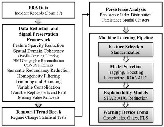
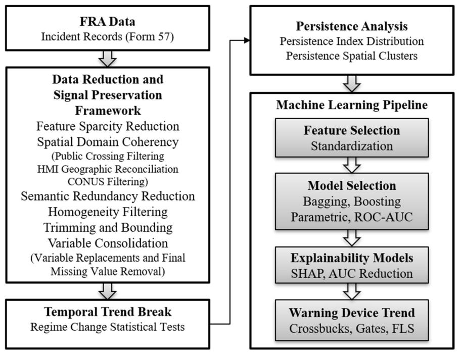
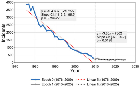
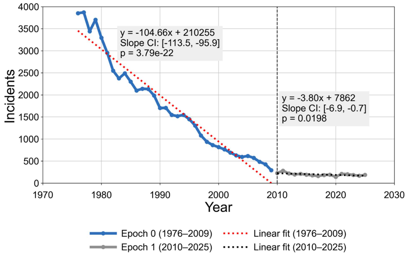
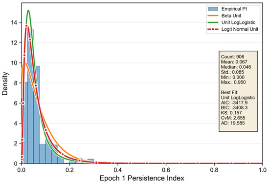
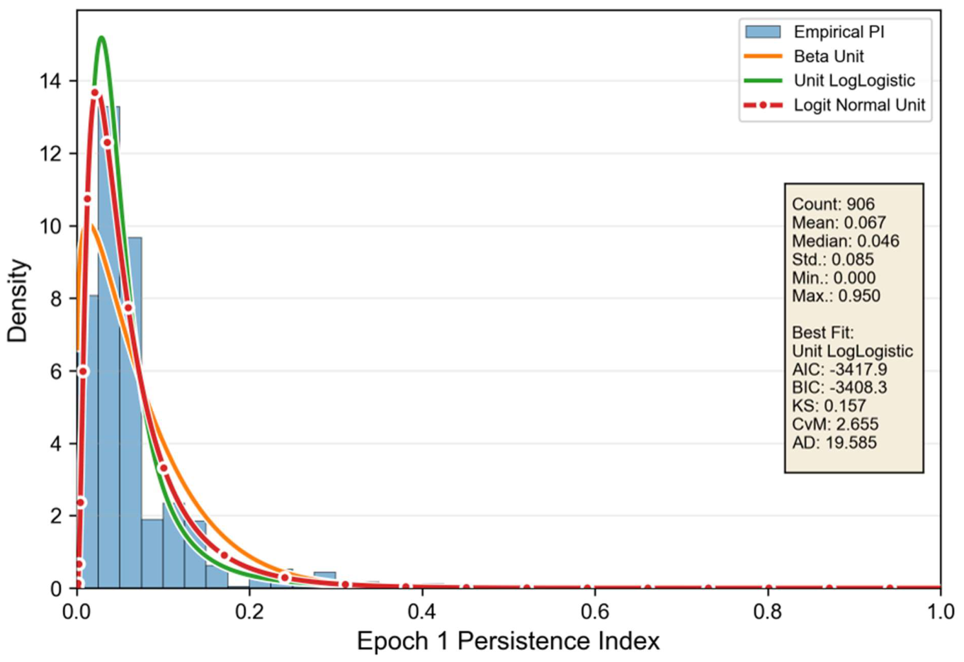
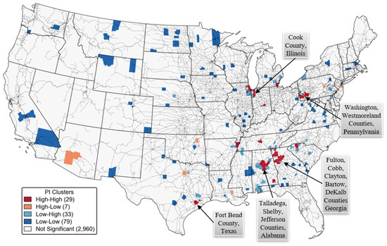
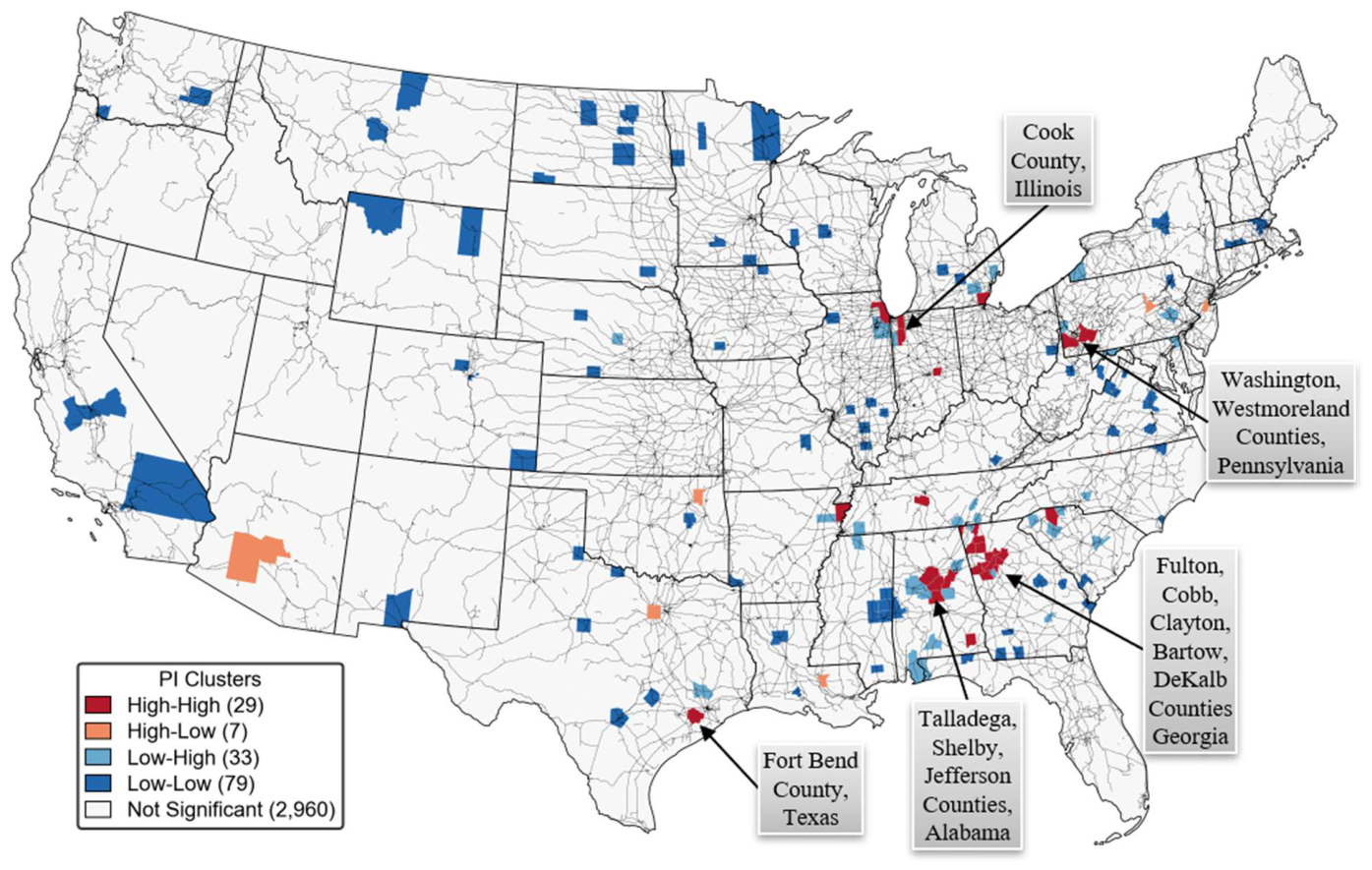
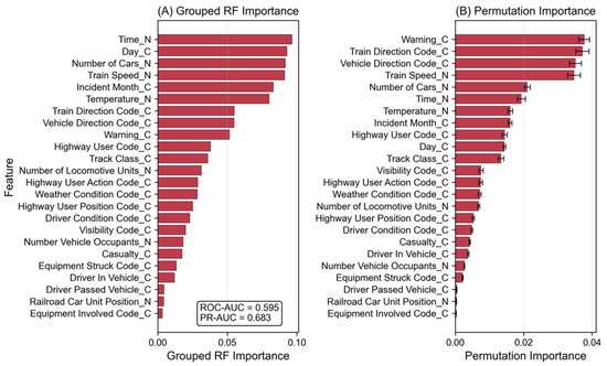
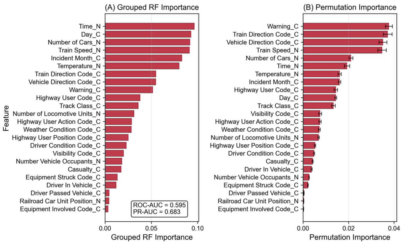
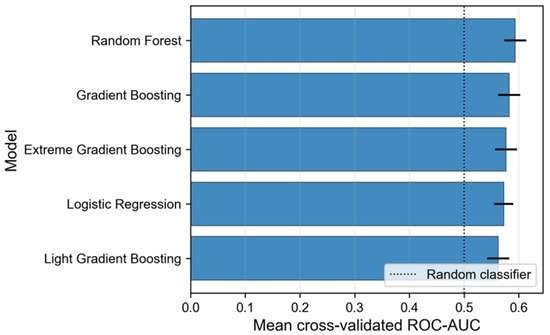
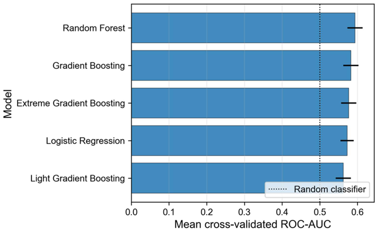
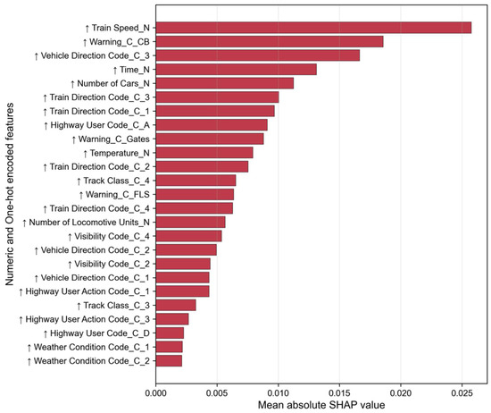
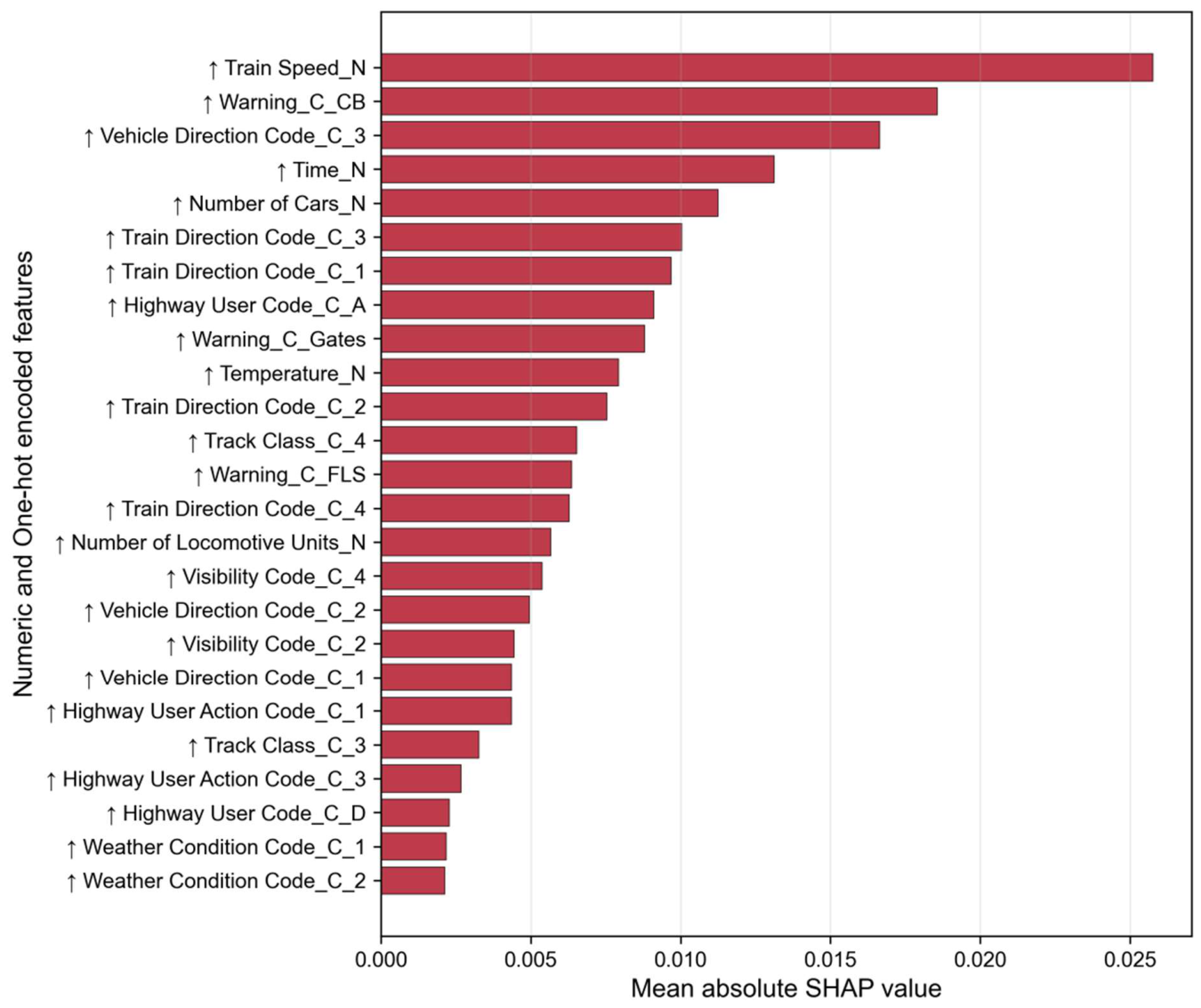
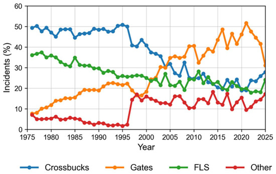
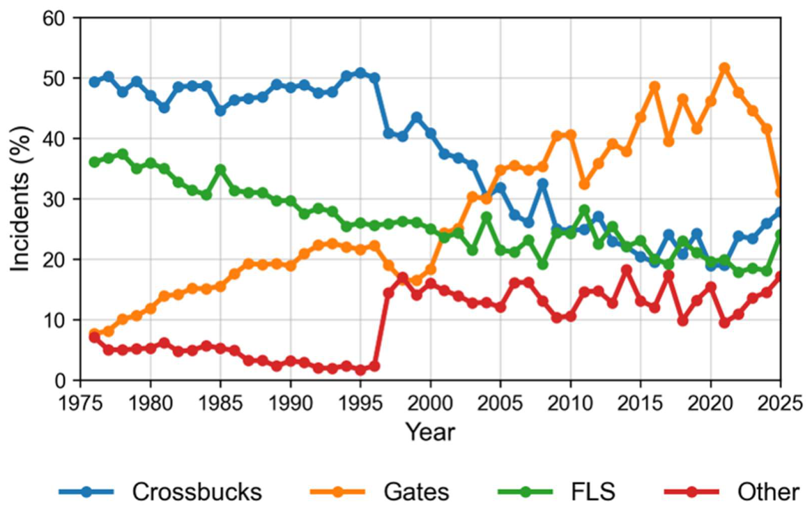

Disclaimer/Publisher’s Note: The statements, opinions and data contained in all publications are solely those of the individual author(s) and contributor(s) and not of MDPI and/or the editor(s). MDPI and/or the editor(s) disclaim responsibility for any injury to people or property resulting from any ideas, methods, instructions or products referred to in the content. |
© 2026 by the author. Licensee MDPI, Basel, Switzerland. This article is an open access article distributed under the terms and conditions of the Creative Commons Attribution (CC BY) license.