DK-VCA Net: A Topography-Aware Dual-Decomposition Framework for Mountain Traffic Flow Forecasting

Abstract

Traffic flow prediction is important for traffic management and safety control in mountainous areas. In these environments, traffic flow is affected by complex terrain, changing weather, and mixed vehicle types, so the resulting time series often show strong fluctuation and poor stability. Many existing prediction models were developed for urban roads or flat highways, and their performance is therefore limited in mountainous scenarios. To address this problem, this paper proposes a hybrid model called DK-VCA Net. The model combines adaptive signal decomposition with a terrain-aware deep learning structure to separate useful traffic variation from complex noise. It also integrates traffic flow, speed, slope, and weather information to better describe mountain traffic conditions. The proposed method is evaluated using real traffic data collected at 5 min intervals from detection stations on the Guibi Expressway in Guizhou Province, China, during September 2020. Experimental results show that DK-VCA Net achieves better prediction accuracy than several representative baseline models, including 1D-CNN, LSTM, Transformer, STWave, and Mamba. Across the 15 min, 30 min, and 60 min forecasting tasks, the proposed model reduces the average RMSE by 14.8% compared with the conventional 1D-CNN model and by 8.9% compared with the baseline Transformer model. The ablation study further proves the effectiveness of the decomposition strategy, terrain-related features, and the attention mechanism. The results show that the proposed method is effective for traffic flow prediction in the studied mountainous highway scenario.

1. Introduction

With the development of the economy and the improvement of living standards, transportation demand has continued to grow. In mountainous areas, traffic congestion has become an increasingly serious problem because of complex terrain and special road conditions. This problem not only reduces the operating efficiency of roads, but also affects regional economic development and daily travel. For this reason, Intelligent Transportation Systems (ITS) are important for improving road network efficiency and easing traffic congestion. Early studies laid the foundation for transportation systems engineering [1]. Traffic flow prediction later became an important part of ITS because it can support signal control and route optimization [2].

Recent studies on traffic flow forecasting can be broadly grouped into three lines: graph-based spatio-temporal models, transformer-based models, and decomposition-based hybrid models. A recent systematic survey also shows that current research is moving toward dynamic graph learning, stronger spatio-temporal coupling, and more practical evaluation settings [3].

Early deep learning studies mainly focused on temporal feature extraction and short-range spatio-temporal coupling. An attention-based Conv-LSTM model showed that combining convolution, recurrence, and attention can improve short-term traffic flow prediction [4]. STGCN further introduced graph convolution into traffic forecasting and showed the value of joint spatial-temporal learning [5]. AGCRN later improved this line by learning adaptive graph relations directly from data [6]. These studies established an important foundation for later spatial–temporal traffic forecasting models, but many of them were still developed for conventional urban traffic scenarios rather than mountainous highways.

Following these developments, graph-based models gradually became a central direction in traffic forecasting research. More recent studies have shown that dynamic spatial dependency modeling helps characterize complex road network interactions, and that graph spatial–temporal transformer frameworks can further improve the learning of coupled spatial and temporal patterns in traffic prediction [7,8]. More recent work such as GSTPRN incorporated spatial position information into recurrent forecasting [9]. Dynamic spatial-aware graph transformer models further extended this line of work by introducing more flexible spatial interactions [7]. These models work well for network-level forecasting, but most of them were developed for urban or regional road networks with relatively dense spatial observations. In mountainous highway scenarios, however, short-term traffic changes are also shaped by local slope variation, tunnel groups, and rapidly changing weather. Under these conditions, spatial correlation alone is often not enough to explain the observed fluctuations.

Transformer-based models have also become an important direction in traffic forecasting because they are effective at modeling long-range temporal dependence. A dynamic and hierarchical transformer model showed that transformer structures can learn complex traffic patterns [10]. Traffic Transformer highlighted the role of continuity and periodicity in traffic sequences [11]. PDFormer further emphasized propagation delay and dynamic long-range dependence in traffic forecasting [12]. STWave combined wavelet-style disentangling with spatio-temporal modeling and achieved strong performance [13]. GSTTN extended transformer modeling to graph-based traffic prediction [8], and a multi-channel spatio-temporal transformer model showed that combining different temporal representations can also be useful [14]. Even so, these models still depend heavily on the quality of the input sequence. When the raw data contain strong high-frequency disturbance and abrupt variance changes, attention-based models may still mix useful traffic evolution with random noise. This problem is more noticeable on mountain highways, where traffic states are more sensitive to terrain and weather conditions.

Another important direction is decomposition-based hybrid forecasting. CEEMDAN provides a way to separate complex signals into components at different scales [15]. VMD further offers a variational framework for extracting band-limited modes from non-stationary signals [16]. Hybrid models that combine CEEMDAN with machine learning have reported better results than direct prediction on raw traffic sequences [17]. Recent traffic forecasting studies have also shown that decomposition-based models can improve prediction under strongly fluctuating conditions [18]. A recent two-stage decomposition study further suggested that strongly fluctuating traffic series require more targeted treatment before prediction [19]. However, many existing studies still rely on single-stage decomposition or treat all decomposed components in the same way. As a result, informative fluctuation and random disturbance may not be sufficiently distinguished, and the model may still suffer from noise fitting in strongly fluctuating scenarios.

Overall, existing studies provide useful tools from different directions. Graph-based methods are effective for spatial dependency modeling, transformer-based methods are strong in capturing long-range temporal patterns, and decomposition-based methods help reduce the influence of non-stationary signals. However, mountain highway traffic combines terrain-induced local disturbance, weather sensitivity, high-frequency fluctuation, and limited data coverage. Therefore, there is still a need for a framework that first improves signal quality and then performs effective temporal modeling under terrain-aware multi-source input.

The choice of CEEMDAN, VMD, 1D-CNN, and attention is based on the characteristics of mountainous highway traffic data. CEEMDAN is first used to separate multi-scale components from the original non-stationary sequence [15]. VMD is then applied only to the high-complexity components because single-stage decomposition is often not sufficient for strong high-frequency disturbance, while decomposing all components again would introduce unnecessary computation [16]. After signal purification, 1D-CNN is used to capture local temporal patterns in mountainous traffic flow. Attention is further introduced because 1D-CNN alone is not sufficient to highlight critical time steps and longer-range temporal influence [4]. Therefore, the proposed architecture is a targeted design for noisy, strongly fluctuating, and terrain-sensitive traffic series rather than a simple combination of existing modules.

The present study is positioned as a scenario-oriented forecasting framework for mountainous highway traffic rather than a general large-scale network forecasting model. Unlike graph-based methods that mainly focus on spatial topology learning, it pays more attention to local disturbance caused by terrain, tunnel groups, and weather changes. Unlike transformer-based methods that directly learn from raw sequences, it introduces signal purification before temporal modeling to reduce the influence of high-frequency disturbance. It also differs from conventional decomposition-based hybrid models by combining selective secondary decomposition with terrain-aware multi-source input and temporal learning. Therefore, the novelty of this work lies in a targeted framework that connects signal purification, terrain-related feature integration, and temporal modeling for mountainous highway traffic forecasting.

The main contributions of this paper are as follows:

• A scenario-oriented forecasting framework called DK-VCA Net is proposed for mountainous highway traffic flow prediction. Unlike existing methods that mainly focus on spatial topology modeling, long-range temporal dependency, or signal decomposition alone, the proposed framework combines selective dual decomposition with terrain-aware temporal learning to handle strong local disturbance and the non-stationary nature of mountainous traffic flow.
• This study develops an adaptive dual-decomposition strategy based on CEEMDAN, K-means clustering, and VMD. The aim is to improve signal purification for strongly fluctuating mountain traffic series without introducing unnecessary full secondary decomposition.
• This study builds a prediction module that combines 1D-CNN with an attention mechanism. The 1D-CNN is used to capture local temporal patterns, while the attention mechanism is added to highlight important time steps that are not easily emphasized by convolution alone.
• Experiments on real highway traffic data from mountainous areas in Guizhou show that the proposed model performs better than the comparison models. Across the 15 min, 30 min, and 60 min forecasting tasks, the proposed model reduces the average RMSE by 14.8% compared with 1D-CNN and by 8.9% compared with Transformer.

The remainder of this paper is organized as follows. Section 2 introduces the main characteristics of mountain traffic flow. Section 3 presents the architecture and key components of the proposed DK-VCA Net. Section 4 describes the experimental setup and reports the comparative results. Section 5 discusses the practical implications of the proposed method. Finally, Section 6 concludes the paper and outlines future research directions.

2. Characteristics of Mountain Traffic Flow

Traffic flow in mountainous areas is usually more complicated than that on urban roads or flat highways. This is mainly because mountainous roads are more strongly affected by terrain, weather, and roadway conditions.

2.1. Traffic Flow Characteristics Due to Topographical Factors

Mountain highways often include long and steep grades, which have a direct effect on vehicle operation. When vehicles travel uphill, they need more traction power, so their speeds generally decrease. At the same time, speed differences between vehicles tend to become more obvious, since different vehicle types respond differently to slope changes. Heavy vehicles are usually influenced more because of their lower power-to-weight ratio, and their speeds often decrease more than those of passenger cars. As a result, traffic flow becomes less stable.

Road alignment in mountainous areas also has an important influence on traffic flow. Sharp curves and frequent tunnel sections make traffic conditions more difficult to describe and predict. In particular, sharp curves and steep grades often reduce drivers’ sight distance, making it harder to observe the road ahead in time and increasing driving risk. For safety reasons, drivers often slow down in advance, which leads to repeated speed changes along the road.

Tunnel sections also affect traffic operation. At tunnel entrances and exits, lighting conditions change quickly, and drivers usually need a short time to adjust. During this process, sudden braking or unstable driving behavior may occur. These disturbances can further trigger kinematic shockwaves and weaken traffic flow stability [20,21].

2.2. Traffic Flow Characteristics Under the Influence of Climatic Conditions

Weather in mountainous areas changes quickly, and heavy rain, snow, and dense fog occur frequently. These weather conditions have a direct impact on road safety because they reduce tire grip and increase braking distance. For example, during heavy rain, water may accumulate on the road surface, which affects vehicle stability and handling. Rainfall can also raise the risk of landslides and mudslides, and in severe cases may even interrupt traffic. Dense fog greatly lowers visibility, so drivers usually reduce speed to stay safe. When many vehicles slow down at the same time, road capacity decreases, and the chances of congestion or rear-end collisions increase [22,23].

Large temperature variations in mountainous areas can also influence vehicle performance and driver behavior. In winter, low temperatures may make engines harder to start, increase fuel consumption, and reduce tire flexibility, which weakens vehicle handling. Cold conditions may also affect drivers’ control of the vehicle and increase the risk of accidents. In summer, high temperatures can lead to engine overheating or tire blowouts. Once these problems occur on narrow mountain roads, the affected vehicles may quickly become local bottlenecks and disrupt normal traffic flow.

2.3. Traffic Flow Characteristics Related to Transportation Infrastructure and Composition

Traffic flow efficiency in mountainous areas is strongly affected by transportation infrastructure. Because road construction in mountainous terrain is difficult and expensive, many mountain roads have narrow sections and limited lane capacity. As traffic demand continues to grow, these roads often have difficulty providing enough carrying capacity. In addition, some roads still lack sufficient safety facilities, such as guardrails, lighting, and clear pavement markings. This can reduce drivers’ sense of safety and also have a negative effect on traffic operation. On many winding mountain roads, overtaking opportunities are limited, so vehicles often need to follow one another over long distances. This lowers travel speed and makes queue formation more likely [1].

Traffic composition in mountainous areas is also more heterogeneous. Passenger cars, trucks, buses, and other vehicle types often share the same road space. Because these vehicles differ in power, operating speed, and driving behavior, traffic flow is more likely to fluctuate. Heavy vehicles are especially affected on long uphill sections due to their lower power-to-weight ratio, and they usually travel at lower speeds. In many cases, they act as moving bottlenecks and slow down the vehicles behind them. In contrast, smaller and more maneuverable vehicles may change lanes or overtake more frequently in order to pass slow vehicles. This can further disturb traffic flow and increase the likelihood of vehicle conflicts.

3. Model Architecture

To deal with the non-stationary and nonlinear characteristics of mountain traffic flow, this paper proposes a model called DK-VCA Net. The model combines a dual-decomposition strategy with a terrain-aware deep learning module. This design makes it easier to separate useful traffic variation from strong environmental disturbance.

3.1. Dual Data Decomposition and Signal Purification

The first part of the model is data preprocessing and signal decomposition. Its main goal is to reduce the strong non-stationary characteristics in raw mountain traffic sequences. Through this process, relatively stable traffic trends can be separated from high-frequency fluctuations caused by terrain and environmental disturbance.

3.1.1. CEEMDAN Decomposition and Physical Interpretation

Complete Ensemble Empirical Mode Decomposition with Adaptive Noise (CEEMDAN) is used as the first decomposition method. It decomposes the complex traffic flow sequence into several Intrinsic Mode Functions (IMFs). Although improved CEEMDAN variants have been reported in recent studies, CEEMDAN is retained here because it provides a stable and interpretable first-stage decomposition for the current data scale, while the subsequent selective VMD stage is used to further refine the most complex components. The detailed mathematical derivation is not repeated here. This section mainly explains what these components mean in mountain traffic scenarios.

For an original traffic flow sequence $f\left(t\right)$, CEEMDAN decomposes it into $K_{\mathrm{IMF}}$ IMFs and one residual term $r\left(t\right)$:

$$f\left(t\right)=\sum _{k=1}^{K_{\mathrm{IMF}}}{\mathrm{IMF}}_k\left(t\right)+r\left(t\right)$$

(1)

where ${\mathrm{IMF}}_k\left(t\right)$ represents components at different temporal scales, and $r\left(t\right)$ represents the overall trend of the traffic flow.

To avoid information leakage during model evaluation, the decomposition settings are fixed using the training set and then applied in the same way to the rolling validation and test windows. In this way, future observations are not introduced into the decomposition of earlier prediction samples.

In mountain traffic scenarios, these decomposed components can be interpreted in a cautious way. Low-frequency IMFs and the residual term mainly reflect slower background variation in traffic demand and road-state evolution. By contrast, high-frequency IMFs are more often associated with short-term fluctuations under local disturbance. These components may be related to sudden speed changes, temporary capacity drops, or other transient effects caused by terrain and weather, but they are not treated here as one-to-one indicators of a single physical source.

By separating long-term traffic trends from terrain-related high-frequency fluctuations, the model can handle the data in a clearer way. This reduces the influence of mixed noise and improves the later deep learning modules. It also makes up for the weakness of traditional end-to-end models when they deal with complex and fast-changing mountain traffic data.

3.1.2. Sample Entropy Calculation and K-Means Clustering

Sample Entropy (SampEn) is used to measure the complexity of the decomposed time-series components. Compared with some traditional entropy measures, SampEn is less affected by sequence length and does not use self-matching. Because of this, it is suitable for short traffic flow sequences. In general, it reflects the irregularity of a sequence. For relatively regular traffic trends, the matching probability decreases slowly as the embedding dimension increases. For more complex signals affected by terrain and environmental disturbance, the matching probability usually decreases faster.

For a finite sequence with length N, embedding dimension m, and similarity tolerance r, SampEn is defined as

$$\mathrm{SampEn}(m,r,N)=-ln\left({\displaystyle \frac{A^{\left(m\right)}\left(r\right)}{B^{\left(m\right)}\left(r\right)}}\right)$$

(2)

where $B^{\left(m\right)}\left(r\right)$ is the probability that two template vectors match in the m-dimensional space within the tolerance threshold r, and $A^{\left(m\right)}\left(r\right)$ is the probability that they still match after the dimension increases to $(m+1)$. In this study, a larger SampEn value means that the corresponding component is more complex. In most cases, this suggests that the component is more likely to contain short-period fluctuation in mountain traffic flow.

Here, a template vector means a short consecutive segment extracted from the original time series. For example, for a sequence $\{x_1,x_2,\dots ,x_N\}$, the i-th template vector in the m-dimensional space can be written as ${\mathbf{X}}_i^{\left(m\right)}=[x_i,x_{i+1},\dots ,x_{i+m-1}]$. Then, $B^{\left(m\right)}\left(r\right)$ is the probability that two template vectors match in the m-dimensional space within the tolerance threshold r, and $A^{\left(m\right)}\left(r\right)$ is the probability that they still match after the dimension increases to $(m+1)$.

After the SampEn value of each Intrinsic Mode Function (IMF) is calculated, K-means clustering is used to classify the IMFs. The SampEn value of each IMF is taken as the clustering input. In this study, the IMFs are divided into three states, namely the trend-dominated state, the transition state, and the noise-dominated state. In this way, the decomposed components can be grouped automatically without setting manual thresholds.

The trend-dominated state mainly contains low-frequency components and is treated as slower background variation in the traffic sequence. The transition state contains middle-frequency components and includes both trend information and fluctuation information. The noise-dominated state mainly contains high-frequency components and is treated as the part that is more likely to contain short-period disturbance. Based on this classification, only the components in the noise-dominated state are sent to the Variational Mode Decomposition (VMD) module for further decomposition, while the other components are kept directly. This helps reduce unnecessary computation and lowers the risk of overfitting to noisy signals.

3.1.3. Adaptive State Selection via K-Means Clustering

In DK-VCA Net, K-means clustering is used as an adaptive state selection method. The purpose of this step is not to further decompose all IMF components in the same way, but to decide which components need additional processing according to their complexity.

The Sample Entropy values obtained in the previous step are used as the basis for clustering. According to the clustering results, the decomposed traffic components are divided into three states with different meanings.

• Trend-dominated state (low complexity): This state mainly contains low-frequency components. In this study, it is treated as slower background variation in the traffic sequence.
• Transition state (medium complexity): This state contains middle-frequency components. It includes both trend information and fluctuation information, and reflects the stage where traffic conditions begin to change.
• Noise-dominated state (high complexity): This state mainly contains high-frequency components. In this study, it is treated as the part that is more likely to contain short-period disturbance and therefore needs further refinement.

With this adaptive classification method, different components can be processed in different ways. The trend-dominated and transition components are kept to preserve the main structure of the traffic sequence. Only the noise-dominated components are sent to the VMD module for further decomposition and denoising. In this way, the second decomposition step is only used where it is needed. This makes the process more efficient and helps the model focus on useful traffic information.

3.1.4. Variational Mode Decomposition for High-Complexity Signals

To further process the high-complexity components selected in the previous stage, this study uses Variational Mode Decomposition (VMD) as the second decomposition method. Compared with some recursive empirical decomposition methods, VMD can reduce error accumulation and mode mixing. It solves a variational optimization problem to decompose the signal, so it works better for high-frequency disturbance in mountain traffic data.

The main goal of VMD is to decompose the selected high-complexity signal, denoted here as $f_{\mathrm{hc}}\left(t\right)$, into several band-limited intrinsic mode functions $u_m\left(t\right)$. Unlike the original traffic flow sequence $f\left(t\right)$ in Equation (1), $f_{\mathrm{hc}}\left(t\right)$ here refers only to the aggregated high-complexity component that is sent to the second decomposition stage. Each mode is centered around a frequency ${\omega }_m$. In this process, the sum of the bandwidths of all modes is minimized, and the reconstructed signal remains close to the original signal. The optimization problem can be written as

$$\begin{array}{cc}\hfill & \underset{\left\{u_m\right\},\left\{{\omega }_m\right\}}{min}\left\{\sum _{m=1}^M{∥{\partial }_t\left[\left(\delta \left(t\right)+{\displaystyle \frac{j}{\pi t}}\right)\ast u_m\left(t\right)\right]e^{-j{\omega }_{m}t}∥}_2^2\right\}\hfill \\ \hfill & \mathrm{s}.\mathrm{t}.\sum _{m=1}^M{u}_m\left(t\right)=f_{\mathrm{hc}}\left(t\right)\hfill \end{array}$$

(3)

where $\left\{u_m\right\}$ and $\left\{{\omega }_m\right\}$ are the decomposed modes and their center frequencies. The term $(\delta \left(t\right)+{\displaystyle \frac{j}{\pi t}})\ast u_m\left(t\right)$ is the analytic signal obtained by the Hilbert transform, which is used to keep a one-sided frequency spectrum.

The standard Alternating Direction Method of Multipliers (ADMM) equations are not repeated here. This paper mainly explains how the method is used in the proposed framework. During optimization, each mode is updated in the frequency domain, and a quadratic penalty factor is used to keep the reconstructed signal close to the original signal. The iteration stops when the squared Euclidean norm of the difference between two consecutive updates is smaller than the preset convergence threshold.

In DK-VCA Net, VMD is only used for the high-complexity components. In this way, useful traffic fluctuation information, such as local braking waves on long steep downhill sections, can be further separated from environmental noise. After that, the purified sub-modes are combined with the preserved low- and mid-complexity components to form a purified multi-channel input sequence for the following terrain-aware deep learning module.

3.2. Fusion of 1D-CNN and Attention Mechanism

3.2.1. Multi-Source Feature Integration and Topography-Aware Input

Different from urban traffic forecasting models that mainly use historical traffic flow data, traffic prediction in mountainous areas also needs to consider weather changes and terrain conditions. To build a terrain-aware input sequence, a historical window with length T is used to construct the multivariate input matrix:

$$\mathbf{X}=[{\mathbf{x}}_{t-T+1},\dots ,{\mathbf{x}}_t]\in {\mathbb{R}}^{T\times d}$$

(4)

where the feature vector at time step t is defined as

$${\mathbf{x}}_t={[F_t,S_t,G_i,W_t]}^T$$

(5)

Here, $F_t$ is the purified traffic flow sequence obtained from the previous dual-decomposition stage. $S_t$ is the average speed at the same time step, and it reflects the local traffic state. $W_t$ is the weather-condition input used in the current dataset, which is encoded as a categorical variable. $G_i$ is the longitudinal slope of the corresponding road segment.

Since $G_i$ is a static terrain feature of a road segment, it is repeated along the time dimension T to keep the same dimension as the dynamic variables. Before feature fusion, all continuous input variables are normalized to reduce the effect of different value ranges, while the weather condition is kept in its categorical form. By combining traffic flow, speed, terrain, and weather information, the input matrix $\mathbf{X}$ provides more complete information for the following deep learning model. This helps the model capture terrain-related traffic fluctuations and weather-related capacity changes better.

3.2.2. 1D-CNN Local Feature Extraction

To extract local features from the terrain-aware input matrix $\mathbf{X}$, stacked one-dimensional convolutional neural network (1D-CNN) layers are used. The convolution operation at layer l can be written as

$$h_j^l\left(p\right)=f\left(b_j^l+\sum _{c=1}^{C_{in}}\sum _{s=1}^K{w}_{j,c}^l\left(s\right)·h_c^{l-1}(p·S+s)\right)$$

(6)

where K and S denote the kernel size and stride, respectively, and the convolution is performed along the temporal dimension.

In this model, the 1D-CNN not only processes traffic flow, but also learns from speed, slope, and weather information at the same time. By moving the convolution kernel along the multi-source input sequence, the network can capture short-term relations among different features. From the traffic flow point of view, this process helps identify local traffic changes, such as the early spread of speed reduction caused by heavy vehicles on long steep slopes.

3.2.3. Attention-Based Dynamic Temporal Reweighting

Although stacked 1D-CNN layers can extract local temporal features, their receptive field is still limited. Because of this, they are not enough to capture long-range dependence in the whole historical window. To solve this problem, the high-level feature representation $\mathbf{H}$ produced by the convolutional layers is sent to a self-attention module. In this module, $\mathbf{H}$ is projected into the Query ($\mathbf{Q}$), Key ($\mathbf{K}$), and Value ($\mathbf{V}$) matrices:

$$\mathbf{Q}=\mathbf{H}{\mathbf{W}}_Q,\mathbf{K}=\mathbf{H}{\mathbf{W}}_K,\mathbf{V}=\mathbf{H}{\mathbf{W}}_V$$

(7)

Here, ${\mathbf{W}}_Q$, ${\mathbf{W}}_K$, and ${\mathbf{W}}_V$ are trainable projection matrices. They are initialized together with the other network parameters and updated jointly through backpropagation during model training [10,11].

Then, temporal weighting is calculated by scaled dot-product attention:

$$\mathrm{Attention}(\mathbf{Q},\mathbf{K},\mathbf{V})=\mathrm{Softmax}\left({\displaystyle \frac{\mathbf{Q}{\mathbf{K}}^T}{\sqrt{d_k}}}\right)\mathbf{V}$$

(8)

In mountain traffic forecasting, the attention mechanism helps the model focus on important time periods. It gives higher weights to time steps where traffic conditions change clearly. This makes it easier for the model to capture sudden disturbances, such as temporary capacity drops caused by bad weather or continuous braking on steep mountain roads. In this way, the attention block acts as a temporal reweighting layer on top of the local features extracted by the 1D-CNN, rather than as a separate prediction branch.

3.2.4. Detailed Network Configuration

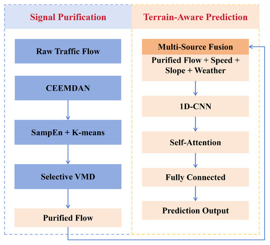
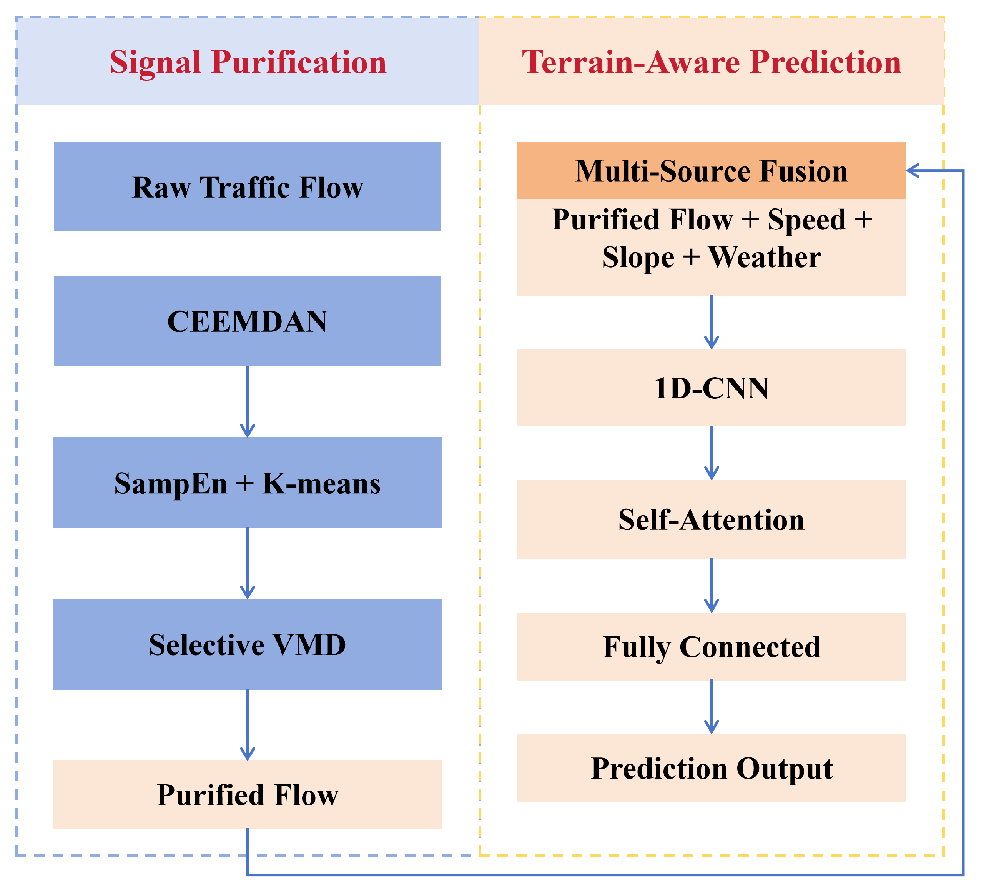
Figure 1 shows the overall framework of DK-VCA Net. The model is composed of two main parts: a signal purification stage and a terrain-aware prediction stage. In the first stage, the raw traffic flow series is purified through a dual-decomposition process. In the second stage, the purified flow is combined with speed, slope, and weather information and then fed into a prediction module built on 1D-CNN and self-attention.

Figure 1. Overall framework of DK-VCA Net. The left part shows the signal purification process based on CEEMDAN, Sample Entropy, K-means clustering, and selective VMD. The right part shows the terrain-aware prediction process using purified flow, speed, slope, and weather information.

For clearer model description and easier reproduction, the main network structure is summarized here. The terrain-aware predictor includes a two-layer 1D-CNN feature extractor, a self-attention block, and a final regression layer. The convolutional layers are used to capture short-term local patterns from the purified multi-source sequence, while the attention block helps emphasize more informative temporal positions before prediction. The detailed network settings are given in Table 1.

Table 1. Detailed network configuration of DK-VCA Net.

Module	Setting
Input	Historical window length $T=12$; input dimension $d=4$ (purified flow, speed, slope, weather)
1D-CNN layer 1	In-channels $=4$; out-channels $=32$; kernel size $=3$; stride $=1$; padding $=1$; activation = ReLU
1D-CNN layer 2	In-channels $=32$; out-channels $=64$; kernel size $=3$; stride $=1$; padding $=1$; activation = ReLU
Dropout	0.2
Attention block	Number of heads $=4$; model dimension $=64$; key/query dimension $d_k=16$; value dimension $d_v=16$
Output layer	Fully connected regression layer; output dimension $=1$

For clarity, Algorithm 1 summarizes the main processing steps of DK-VCA Net from signal purification to final prediction.

Algorithm 1 Main procedure of DK-VCA Net

1: Input raw traffic flow sequence F, speed sequence S, slope feature G, and weather feature W   2: Split the dataset into training, validation, and test sets in time order   3: Apply CEEMDAN to the training traffic flow sequence and obtain IMF components and residual   4: Compute Sample Entropy for each IMF   5: Use K-means to divide the IMF components into trend-dominated, transition, and noise-dominated groups   6: Keep the trend-dominated and transition components directly   7: Apply VMD only to the noise-dominated component group and obtain purified sub-modes   8: Reconstruct the purified traffic flow sequence $F*$ from the preserved components and purified sub-modes   9: Build the multi-source input matrix $\mathbf{X}=[F*,S,G,W]$ 10: Feed $\mathbf{X}$ into stacked 1D-CNN layers to extract local temporal features 11: Send the high-level representation to the self-attention module for temporal reweighting 12: Use the output layer to generate traffic flow prediction 13: Optimize the network parameters on the training set and tune hyperparameters on the validation set 14: Report prediction results on the test set

Algorithm 1 provides a compact summary of the complete processing pipeline used in the proposed framework.

4. Simulation Experiments

4.1. Data Source and Characteristics

The traffic data used in this study were collected from vehicle detection stations along the Guibi Expressway in Guizhou Province, China. This expressway passes through a typical mountainous area, and the data were recorded at 5 min intervals during September 2020. In this study, the dataset is used as a real-world case from a mountainous corridor for controlled method validation. Since the observation period covers only one month, it does not reflect seasonal changes such as winter ice and snow, spring fog, or summer rainstorms. For this reason, the present results are not intended to demonstrate seasonal generalizability, and further validation with longer-term data is still needed.

The model inputs include four types of features related to traffic operation in mountainous areas:

• Traffic Flow (veh/5 min): This is the prediction target and describes the temporal variation in traffic volume.
• Average Speed (km/h): This variable reflects the operating condition of traffic and local congestion levels.
• Slope Gradient (%): This variable describes the longitudinal slope of a road segment and is used to represent the influence of uphill and downhill conditions on vehicle movement, especially for heavy vehicles on long continuous grades.
• Weather Condition: This feature is encoded as a categorical variable, where 0 denotes normal or sunny weather, 1 denotes rainy weather, and 2 denotes foggy or snowy weather. It is used to represent the effect of weather changes on traffic flow.

In the current dataset, weather information is available only in the form of synchronized categorical labels rather than continuous meteorological measurements. Therefore, weather categories are used here as the most consistent environmental input available for the study corridor. This representation can reflect broad differences in traffic conditions under different weather states, but it cannot capture more detailed meteorological effects such as rainfall intensity, visibility, temperature changes, or wind speed.

Before model training, the detector records were examined for duplicated timestamps, incomplete entries, and obvious abnormal values. Records missing essential fields were removed before temporal aggregation, and the remaining data were aggregated into 5 min intervals. To avoid temporal leakage, the dataset was divided in chronological order into a training set (70%), a validation set (10%), and a testing set (20%). All continuous dynamic features were normalized by Min-Max scaling based only on the statistics of the training set, while the weather condition was retained as a categorical variable encoded as 0, 1, and 2. The statistical characteristics of the dataset are summarized in Table 2. Among all samples, adverse weather conditions account for about 27.5%.

Table 2. Statistical summary of the experimental dataset.

Feature Attribute	Min	Max	Mean ± Std
Traffic Flow (veh/5 min)	0	385	$142\pm 45$
Average Speed (km/h)	25.4	110.2	$78.5\pm 12.6$
Slope Gradient (%)	0.5	5.8	$3.2\pm 1.4$
Weather Condition	Count (Percentage)
Sunny/Cloudy (Normal)	12,450 (72.5%)
Rainy	3200 (18.6%)
Foggy/Snowy (Adverse)	1528 (8.9%)

The dataset used in this study provides a real mountainous highway case for controlled validation, but it is still limited to one corridor and one month. Therefore, the conclusions of this paper should be understood as evidence for this specific scenario rather than as universal claims across all road networks and seasons. In addition, only four variables, namely traffic flow, speed, slope, and weather condition, are used in the present study because they were available in a consistent and synchronized form for the study corridor. Other potentially relevant factors, such as incidents, traffic control conditions, and driver behavior, were not included in the current dataset and are treated as limitations of the present study rather than ignored effects.

4.2. Dual Decomposition and Complexity Analysis

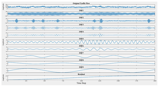
To reduce the strong non-stationary characteristics of mountain traffic flow, the original traffic flow sequence is first decomposed by CEEMDAN. In this study, the noise standard deviation is set to 0.2, and the number of ensemble iterations is set to 5000. After decomposition, a series of Intrinsic Mode Functions (IMFs) and one residual term are obtained, as shown in Figure 2.

Figure 2. CEEMDAN decomposition results of mountain traffic flow.

Figure 2 shows that the fluctuation amplitude gradually decreases from IMF1 to the residual term, which is consistent with the multi-scale fluctuation structure of mountain traffic flow. Then, Sample Entropy (SampEn) is calculated to measure the complexity of each decomposed component. In this study, the embedding dimension is set to $m=2$, and the similarity tolerance is set to $r=0.2$. As shown in Table 3, a larger entropy value means that the corresponding component is more complex and more irregular. In mountain traffic scenarios, these high-entropy components are more often associated with short-term disturbances, such as local speed changes on steep slopes or temporary traffic capacity drops caused by dense fog.

Table 3. Sample entropy values of CEEMDAN components.

IMF Component	SampEn	IMF Component	SampEn
IMF1	2.45	IMF6	0.86
IMF2	1.98	IMF7	0.69
IMF3	1.45	IMF8	0.45
IMF4	1.32	IMF9	0.21
IMF5	1.21	RES	0.005

To avoid giving the decomposed components overly definite physical interpretations, a frequency-domain check is also performed. The Fourier spectra indicate that the early IMFs mainly contain shorter-period fluctuations, while the later IMFs and the residual term are dominated by slower variations. This suggests that the decomposition is reasonable from a signal-analysis perspective, but it should not be understood as implying a strict one-to-one relation between a given IMF and a specific terrain factor. In this study, the decomposition is therefore used mainly as a multi-scale signal separation tool rather than as a direct physical identification method. The main frequency ranges of these component groups are summarized qualitatively in Table 4.

Table 4. Qualitative spectral summary of CEEMDAN components.

Component Group	Dominant Period Range	Interpretation Used in This Study
IMF1–IMF3	10–30 min	Short-period local fluctuation
IMF4–IMF6	30–90 min	Transition-scale variation
IMF7–RES	>90 min	Slower background variation

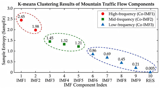
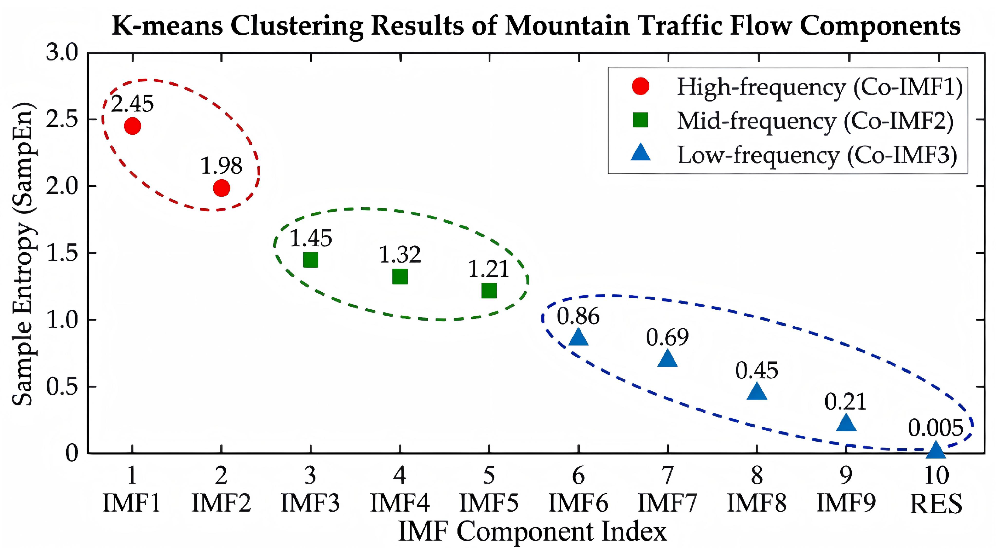
Using the calculated SampEn values as one-dimensional input features, the K-means algorithm divides the IMFs into three states: the trend-dominated state (low frequency), the transition state (middle frequency), and the noise-dominated state (high frequency), as shown in Figure 3.

Figure 3. K-means clustering results of mountain traffic flow components.

To further reduce noise interference and keep the computational cost low, secondary Variational Mode Decomposition (VMD) is only used for the high-complexity noise-dominated component group, denoted as $\mathit{Co-I}M{F}_1$ after clustering. Here, $\mathit{Co-I}M{F}_1$ refers to the cluster label of the high-complexity component group rather than to the original first IMF component alone. In this study, the number of VMD modes is set to $M=9$. With this step, useful traffic fluctuation information can be further separated from complex environmental noise.

4.3. Baseline Models and Evaluation Metrics

To evaluate the performance of DK-VCA Net, seven baseline models are selected for comparison. These models include common temporal prediction methods, graph-based spatio-temporal models, and recent advanced sequence models:

• 1D-CNN: A basic temporal convolutional network that uses the same multi-source input matrix. It is used to show the effect of signal decomposition.
• LSTM: A classic Long Short-Term Memory network that is widely used in time-series forecasting.
• STGCN: A representative graph-based spatio-temporal forecasting model that combines graph convolution with temporal convolution.
• AGCRN: An adaptive graph convolutional recurrent network that can learn graph relations from data.
• Transformer: A standard self-attention model that can capture long-range dependence, but does not consider terrain-related information.
• STWave: A spatiotemporal prediction model designed to describe wave-like traffic propagation. It is used as an advanced comparison model.
• Mamba: A state-space sequence model with high computational efficiency. It is used as another advanced comparison model for complex time-series prediction.

Among these baselines, STGCN and AGCRN are included as representative graph-based spatial–temporal models to provide a direct reference for spatial dependency learning under the current corridor-level data setting. At the same time, the proposed DK-VCA Net is not formulated as a graph model in the present study, and its current scope is station-wise forecasting with terrain-aware multi-source input. The present quantitative comparison therefore focuses on reproducible baselines that can be trained under the same data setting and with the same core input structure. Some mountain-road studies reported in the literature are based on site-specific rule systems, fuzzy models, or external measurements that are not available in synchronized form in the current dataset. For this reason, these methods are not included here as direct quantitative baselines, and their relevance to mountainous traffic forecasting is discussed qualitatively in the revised manuscript.

The prediction performance is evaluated by three common metrics: Mean Absolute Error (MAE), Root Mean Square Error (RMSE), and Mean Absolute Percentage Error (MAPE). MAE measures the average absolute deviation between prediction and observation. RMSE gives higher penalty to large errors and is therefore useful for evaluating performance under sudden fluctuations. MAPE reflects the relative prediction error and is used to compare performance under different traffic levels. These three metrics are used together to provide a more balanced evaluation of overall accuracy, sensitivity to large deviations, and relative robustness.

4.4. Hyperparameter Settings and Training Configuration

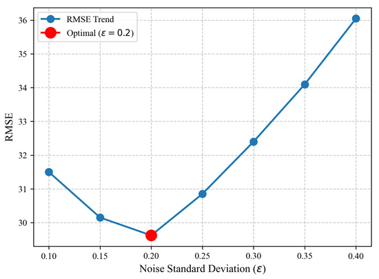
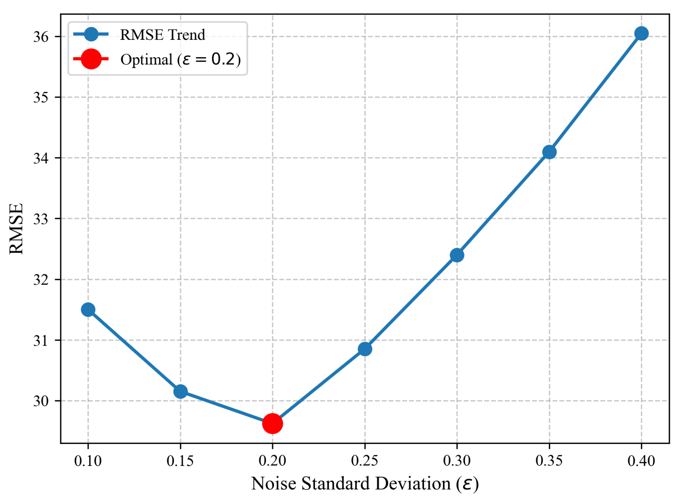
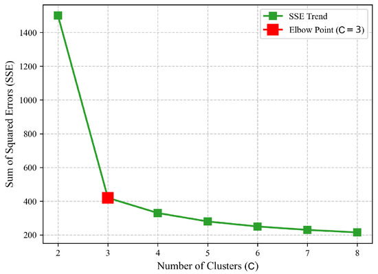
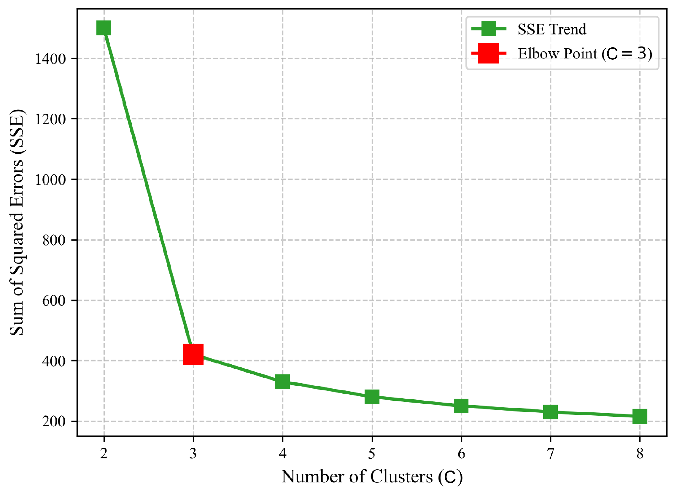
The main hyperparameters in DK-VCA Net are selected according to signal characteristics and validation performance. For the decomposition stage, the CEEMDAN noise standard deviation $\epsilon$ and the K-means cluster number are tuned by sensitivity analysis. As shown in Figure 4, the RMSE reaches its lowest value when $\epsilon =0.2$. Figure 5 shows that $C=3$ is a suitable choice for separating the decomposed components into trend-dominated, transition, and noise-dominated states.

Figure 4. RMSE vs. $\epsilon$ in CEEMDAN.

Figure 5. SSE vs. Cluster Number C.

The remaining parameters are fixed according to stable empirical settings and validation performance. In the CEEMDAN stage, the number of ensemble iterations is set to 5000.

In the SampEn stage, the embedding dimension and similarity tolerance are set to $m=2$ and $r=0.2$, respectively. The choice $m=2$ is used because the traffic sequences in each rolling window are relatively short, and a larger embedding dimension would reduce the number of effective template matches and make the entropy estimate less stable. The tolerance $r=0.2$ is used as a moderate similarity threshold to balance sensitivity to local fluctuations and matching stability in short time-series analysis.

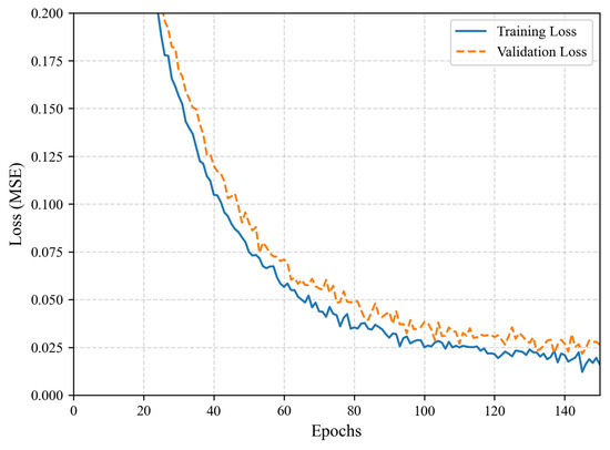
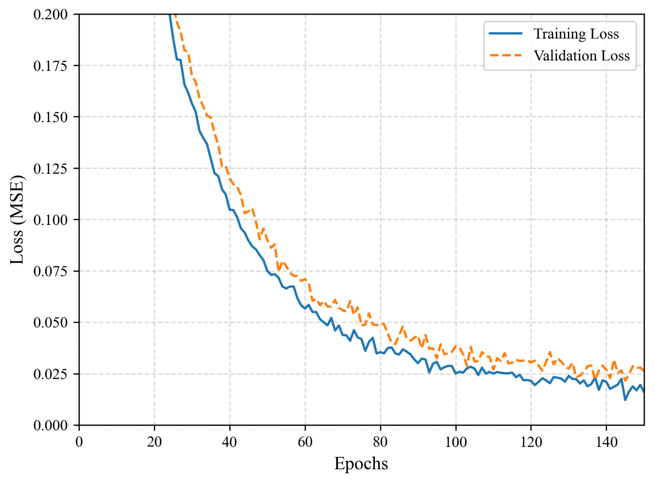
In the VMD stage, the number of modes for the high-complexity component is set to $M=9$, with a penalty factor of 2000 and a convergence tolerance of ${10}^{-7}$. During network training, the Adam optimizer is used with an initial learning rate of 0.001 and a batch size of 64. The detailed hyperparameter settings are given in Table 5. As shown in Figure 6, the loss gradually stabilizes within 150 epochs, and the gap between the training and validation losses remains small during training.

Table 5. Main hyperparameter settings in DK-VCA Net.

Module	Parameter	Value
CEEMDAN	Noise standard deviation $\epsilon$	0.2
CEEMDAN	Ensemble iterations	5000
SampEn	Embedding dimension m	2
SampEn	Similarity tolerance r	0.2
K-means	Number of clusters C	3
VMD	Number of modes M	9
VMD	Penalty factor $\alpha$	2000
VMD	Convergence tolerance	${10}^{-7}$
Training	Optimizer	Adam
Training	Initial learning rate	0.001
Training	Batch size	64
Training	Maximum epochs	150

Figure 6. Training and validation loss curves.

These parameter settings are determined based on the current corridor-level dataset and are not intended to be directly applied to all mountainous highways. Whether they remain effective under different slope conditions, tunnel distributions, and altitude environments still needs to be examined with data from more road corridors.

The convergence curves indicate that the validation loss decreases along with the training loss and does not show clear divergence in the later training stage. This suggests that, under the chronological training-validation-test split adopted in this study, the current model does not exhibit obvious overfitting.

To make the experiments easier to reproduce, all decomposition parameters, network settings, and training hyperparameters are reported explicitly. The dataset is divided in a fixed chronological order, and the same training, validation, and test sets are used for all compared models. The proposed model is implemented in PyTorch 2.0.1 and trained under the same computational environment as the baseline models so that the comparison remains consistent.

4.5. Complexity and Scalability Analysis

Besides prediction accuracy, computational cost is also an important factor in practical deployment. Table 6 compares DK-VCA Net with the baseline models in terms of parameter count, floating-point operations (FLOPs), and average inference time per sample. The parameter count and FLOPs are reported for the prediction network, while the inference time is measured for the complete prediction pipeline under the same experimental environment.

Table 6. Complexity comparison of different forecasting models.

Model	Params (M)	FLOPs (G)	Inference Time (ms/Sample)
1D-CNN	0.18	0.021	1.52
LSTM	0.41	0.036	2.34
STGCN	0.56	0.049	3.21
AGCRN	0.64	0.055	3.47
Transformer	1.31	0.119	5.83
STWave	0.97	0.087	4.76
Mamba	0.73	0.063	3.08
DK-VCA Net	0.52	0.058	3.86

As shown in Table 6, DK-VCA Net is not the lightest model, but its complexity remains moderate. Compared with 1D-CNN and LSTM, the proposed model introduces additional cost because of the decomposition stage and the attention module. However, it is still clearly lighter than Transformer and STWave in both parameter count and FLOPs, and its inference time remains within a short online forecasting interval. This is mainly because the second decomposition stage is applied only to the high-complexity component rather than to all components, which limits the extra computational burden.

From a computational point of view, the temporal convolution stage scales approximately as $O(T·k·C_{\mathrm{in}}·C_{\mathrm{out}})$, while the self-attention stage scales as $O(T^2·d)$. The additional decomposition cost is higher than that of direct end-to-end models, but the selective VMD strategy reduces this burden by refining only the most complex component instead of all decomposed components. This design explains why DK-VCA Net is slower than 1D-CNN and LSTM, but still remains competitive with Mamba and clearly lighter than Transformer and STWave under the current corridor-level setting.

4.6. Predictive Performance and Comparative Analysis

4.6.1. Comparison with State-of-the-Art Baselines

To further evaluate the performance of DK-VCA Net, this section compares it with several baseline models under different forecasting horizons. These models include traditional deep learning methods (1D-CNN and LSTM), an attention-based model (Transformer), hybrid prediction models (ARIMA-LSTM and CEEMDAN-LSTM), and recent advanced models (STWave and Mamba). To make the comparison fair, all models are trained and tested under the same settings, including data division, training epochs, and optimization method.

Table 7 reports the prediction results under three forecasting horizons: 15, 30, and 60 min. A separate model is trained for each forecasting horizon, so the output dimension of the regression layer remains 1 in each run.

Table 7. Comparison of Prediction Accuracy with State-of-the-Art Baselines.

Horizon	Metric	1D-CNN	LSTM	STGCN	AGCRN	Transformer	ARIMA-LSTM	CEEMDAN-LSTM	STWave	Mamba	DK-VCA Net
15 min	MAE	19.56	18.92	18.46	18.24	18.05	17.84	17.62	17.45	17.38	17.10
	RMSE	36.59	33.15	32.40	31.86	31.50	30.94	30.21	29.50	29.35	28.74
	MAPE	12.39	13.56	12.88	12.54	12.15	11.98	11.76	11.55	11.48	11.20
30 min	MAE	20.65	21.45	20.58	20.31	20.12	19.74	19.50	19.35	19.22	18.96
	RMSE	49.27	45.80	44.72	44.10	43.25	42.67	41.96	41.10	40.80	39.85
	MAPE	19.35	18.10	17.48	17.05	16.40	16.05	15.88	15.65	15.45	15.20
60 min	MAE	28.26	26.85	25.96	25.52	25.15	24.73	24.20	24.05	23.95	23.80
	RMSE	65.92	58.60	55.70	54.90	52.40	51.73	50.88	49.50	48.80	47.26
	MAPE	23.45	21.50	20.10	19.65	18.12	17.84	17.35	17.15	16.90	16.70
Average	MAE	23.52	22.41	21.67	21.36	21.11	20.77	20.44	20.28	20.18	19.95
	RMSE	45.33	45.85	44.27	43.62	42.38	41.78	41.02	40.03	39.65	38.62
	MAPE	16.34	17.72	16.82	16.41	15.56	15.29	14.99	14.78	14.61	14.37

As shown in Table 7, DK-VCA Net gives the best prediction results under all forecasting horizons. It has the lowest MAE, RMSE, and MAPE values in the 15 min, 30 min, and 60 min prediction tasks.

For the 15 min forecasting horizon, STGCN and AGCRN already improve the results over 1D-CNN and LSTM, which indicates that graph-based spatial modeling is beneficial even for a mountainous corridor. However, DK-VCA Net still performs better. For example, its RMSE is 28.74, which is lower than that of AGCRN (31.86), Transformer (31.50), and Mamba (29.35). This shows that the proposed model can better reduce the influence of short-term high-frequency disturbance in mountain traffic data.

When the forecasting horizon becomes longer, the prediction errors of all models increase. At the 60 min horizon, AGCRN reduces the RMSE to 54.90, Transformer further reduces it to 52.40, and STWave and Mamba reduce it to 49.50 and 48.80, respectively. DK-VCA Net further reduces the RMSE to 47.26, which shows that it keeps better prediction stability in longer forecasting tasks.

The better performance of DK-VCA Net across different forecasting horizons is consistent with the design of the proposed framework. At shorter horizons, the decomposition stage helps suppress high-frequency disturbance and improves short-term tracking ability. At longer horizons, the attention module contributes more by highlighting informative temporal positions over the historical window. This explains why the proposed model maintains a larger advantage when the forecasting horizon increases. The results therefore support the design choice of combining selective signal purification with temporal reweighting for mountainous traffic prediction.

4.6.2. Robustness Under Noisy and Adverse-Weather Scenarios

To further examine the robustness of DK-VCA Net, two additional experiments are conducted. The first experiment evaluates model stability under noisy input conditions. Gaussian noise with different intensity levels is added to the traffic flow input, and the resulting RMSE changes are compared across models. The second experiment evaluates model performance on adverse-weather samples only, including rainy and foggy conditions. These two tests are used to examine whether the proposed framework remains stable when the input quality becomes worse or when traffic disturbance becomes stronger.

As shown in Table 8, all models suffer from performance degradation when noise is added to the input sequence. However, DK-VCA Net has the smallest RMSE increase among all compared models. This result shows that the decomposition stage helps reduce the influence of noisy observations on model performance. As reported in Table 9, the proposed model also performs best under adverse-weather conditions, indicating that it maintains relatively stable prediction performance when traffic states are subject to stronger environmental disturbances.

Table 8. Robustness comparison under noisy input conditions.

Model	Clean RMSE	RMSE (+5% Noise)	RMSE (+10% Noise)
1D-CNN	25.62	27.54	29.98
LSTM	22.85	24.31	26.58
STGCN	21.68	23.09	25.37
AGCRN	21.12	22.48	24.71
Transformer	20.40	21.96	24.12
STWave	19.15	20.49	22.44
Mamba	18.80	20.14	22.09
DK-VCA Net	17.50	18.61	20.24

Table 9. Prediction performance under adverse-weather conditions.

Model	MAE	RMSE	MAPE (%)
1D-CNN	25.38	34.92	18.76
LSTM	22.67	31.44	16.92
STGCN	21.94	30.61	16.31
AGCRN	21.47	29.98	15.87
Transformer	20.42	28.73	15.02
STWave	19.36	27.41	14.20
Mamba	18.95	27.02	13.96
DK-VCA Net	17.88	25.64	12.85

4.6.3. Error Analysis and Failure Cases

Although DK-VCA Net achieves the best overall results, relatively large prediction errors can still be observed in some periods with rapid traffic changes. These cases mainly occur when the traffic state changes sharply within a short time, especially under the combined influence of terrain disturbance and weather variation. Under such conditions, the model may still produce slight lag or underestimation around local turning points. This shows that, while the proposed framework improves robustness under complex fluctuations, sudden transitions in mountain traffic flow remain difficult to predict.

4.6.4. Prediction Interval Analysis with Monte Carlo Dropout

To further describe predictive uncertainty in risk-sensitive traffic management, a lightweight prediction interval analysis is conducted using Monte Carlo dropout. In this setting, the dropout layer remains active during inference, and the model performs 30 stochastic forward passes for each input sample. The predictive mean is computed as the average of the stochastic outputs, and the uncertainty range is estimated from their standard deviation.

Let ${\widehat{y}}^{\left(n\right)}$ denote the prediction from the n-th stochastic forward pass. The predictive mean is given by

$$\overline{y}={\displaystyle \frac{1}{N}}\sum _{n=1}^N{\widehat{y}}^{\left(n\right)}$$

(9)

and the predictive standard deviation is

$$\sigma =\sqrt{{\displaystyle \frac{1}{N}}\sum _{n=1}^N{\left({\widehat{y}}^{\left(n\right)}-\overline{y}\right)}^2}$$

(10)

where $N=30$ in this study. Based on these results, the 95% prediction interval is constructed as

$$[\overline{y}-1.96\sigma ,\overline{y}+1.96\sigma ]$$

(11)

The interval quality is evaluated by the Prediction Interval Coverage Probability (PICP) and the Mean Prediction Interval Width (MPIW). PICP measures the proportion of true observations covered by the interval, while MPIW reflects the average width of the prediction interval. A reliable uncertainty estimate should achieve reasonably high coverage without producing excessively wide intervals.

As shown in Table 10, the prediction interval becomes wider as the forecasting horizon increases, which is consistent with the higher uncertainty of longer-term prediction. At the same time, the interval coverage remains above 90% under all three forecasting horizons. These results indicate that DK-VCA Net can provide not only point predictions, but also a reasonable uncertainty range that may be useful for practical traffic management.

Table 10. Prediction interval performance of DK-VCA Net under different forecasting horizons.

Horizon	PICP (%)	MPIW
15 min	93.4	18.52
30 min	92.1	24.87
60 min	90.8	32.41

4.6.5. Ablation Study and Module Analysis

An ablation study is further conducted to examine the role of the main components in DK-VCA Net. The analysis considers four aspects: terrain-aware input, signal decomposition, selective secondary decomposition, and attention-based temporal reweighting. These components are removed one at a time, and the corresponding changes in prediction performance are then compared. The average prediction errors of the resulting model variants are reported in Table 11.

Table 11. Ablation Study Results (Averaged over all forecasting horizons).

Model Variant	RMSE	MAE	MAPE (%)	Cumulative Improvement
1D-CNN (w/o Topography-Aware Features)	47.12	24.63	17.08	-
1D-CNN (with Slope & Weather)	45.73	23.52	16.34	+2.9%
DK-VCA Net (w/o Decomposition)	42.23	22.10	15.36	+10.4%
DK-VCA Net (w/o Secondary Decomp)	40.85	21.35	14.92	+13.3%
DK-VCA Net (w/o Attention)	40.52	21.02	14.78	+14.0%
DK-VCA Net (Full Architecture)	39.69	20.53	14.43	+15.8%

• Effect of Topography-Aware Features: This part examines the influence of terrain and weather information in the model. When only traffic flow and speed are used as inputs, without slope and weather features, the RMSE is 47.12. After slope and weather information are introduced, the RMSE decreases to 45.73, corresponding to an improvement of 2.9%. This result shows that terrain-related features are helpful for representing traffic variation in mountainous areas.
• Necessity of Signal Decomposition: When the raw mountain traffic sequence is used directly as model input without decomposition, the RMSE increases to 42.23. This suggests that direct prediction on the raw sequence is more easily affected by fluctuations and noise. By contrast, signal decomposition helps reduce the influence of non-stationary disturbances before model training.
• Advantage of the Dual-Decomposition Paradigm: To examine the role of the adaptive K-means and VMD modules, a variant using only single-stage CEEMDAN (w/o Secondary Decomp) is also evaluated. Its RMSE decreases to 40.85 compared with the model without decomposition, but it remains higher than that of the full model. This indicates that single-stage decomposition can improve signal quality to some extent, but it is still not sufficient to separate complex noise from useful traffic information. After the second decomposition step is introduced, the prediction error is further reduced.
• Impact of Dynamic Temporal Attention: When the self-attention module is removed (w/o Attention), the RMSE rises to 40.52. This result suggests that the attention mechanism helps the model assign more weight to informative historical time steps. It is particularly useful for capturing traffic variation near key transition periods, such as the early stage of congestion formation on steep downhill sections.

The complete DK-VCA Net integrates these modules into a unified prediction framework for mountain traffic flow and achieves the lowest RMSE of 39.69. In the ablation experiment, its RMSE is 15.8% lower than that of the baseline multivariate 1D-CNN model.

5. Discussion and Practical Implications

The role of DK-VCA Net in mountain traffic prediction is discussed below with the help of visualization results.

(1)

Noise Filtering for Terrain Complexity: Traffic flow in mountainous areas usually contains strong high-frequency fluctuations, which are often associated with terrain changes and possible sensor disturbance. By combining CEEMDAN and VMD, the dual-decomposition method separates these fluctuations from the main traffic trend. This helps reduce environmental noise and allows the model to focus more on useful traffic information.

(2)

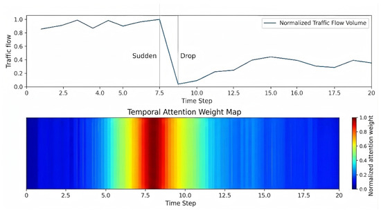
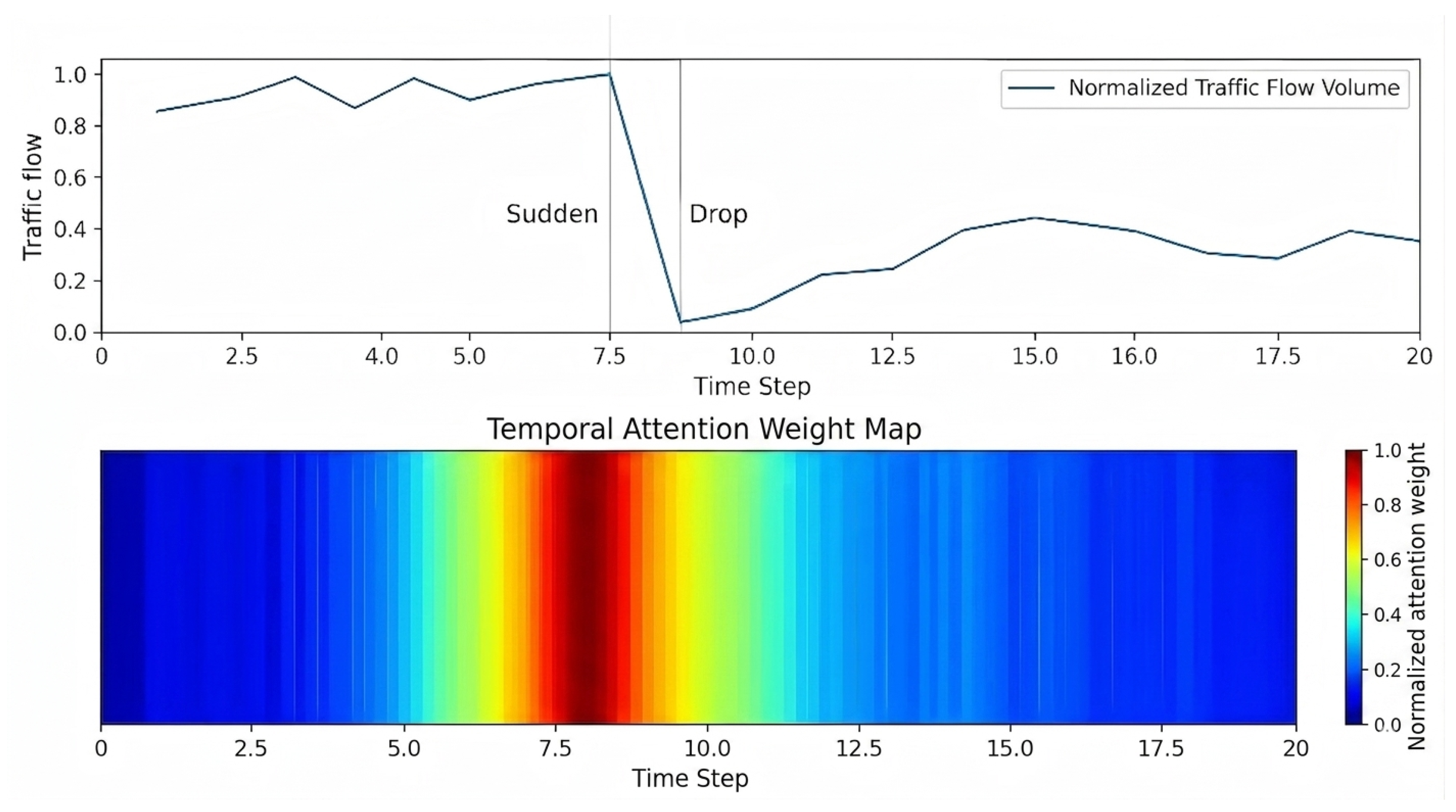
Attention to Critical Events: Figure 7 shows the behavior of the self-attention module. On mountain roads, especially in sections with tunnel groups or rapidly changing weather, traffic states are often unstable. As shown in the upper part of the figure, traffic flow drops sharply between time steps 7 and 9. In the heatmap below, a clear high-attention region appears at the same time. The lower panel visualizes the one-dimensional temporal attention weights by repeating them along the vertical direction. Therefore, the horizontal axis represents time step, while the color intensity represents the normalized attention weight, with warmer colors indicating higher attention. This suggests that the attention mechanism can focus on sudden traffic changes and give more weight to important abnormal events.

Figure 7. Visualization of the attention mechanism under sudden traffic changes. The upper panel shows a sample normalized traffic flow sequence, in which a clear drop appears between time steps 7 and 9. The lower panel shows the corresponding temporal attention weights in a heatmap form. The horizontal axis denotes the time step, and the color intensity represents the normalized attention weight, with warmer colors indicating higher attention. For clearer visualization, the one-dimensional attention weight vector is repeated along the vertical direction.

It should also be noted that some mountain-road studies in the literature focus on site-specific forecasting strategies, such as rule-based or fuzzy formulations under particular weather and terrain conditions. These studies are valuable for understanding mountain traffic characteristics, but many of them rely on data inputs or operational assumptions that are not directly matched by the present dataset. For this reason, the current manuscript keeps the quantitative comparison within a common and reproducible experimental setting, while domain-specific mountain-road studies are treated as an important direction for future comparative evaluation.

In addition to prediction accuracy, a reliable prediction model is also important for traffic management and control in Intelligent Transportation Systems (ITS). The results of this study show that the proposed model has practical value for mountain highway management:

(1)

Proactive Congestion Warning Systems: Traditional traffic management mainly depends on real-time monitoring, so measures are often taken only after congestion has already occurred. Because DK-VCA Net still maintains reasonable prediction accuracy at the 60 min forecasting horizon, traffic control centers can identify possible bottlenecks earlier. Managers then have more time to prepare response measures and send warning information through navigation platforms before serious congestion forms.

(2)

Dynamic Control in Hazard Zones: Mountain highways often include long downhill sections and tunnel groups. In these sections, traffic safety risks are high because speed differences between vehicles are often large. By predicting short-term traffic flow changes and reducing the influence of noise, the model output can be combined with upstream Variable Message Signs (VMS). When the model predicts a rapid increase in traffic flow entering a risk-prone section, managers can adjust the speed limit in advance to reduce traffic disturbance and lower the risk of rear-end crashes.

(3)

Data-Driven Infrastructure Planning: The dual-decomposition framework can also show different types of traffic fluctuations on mountain roads. Low-frequency components reflect more stable traffic demand patterns, such as repeated congestion during peak hours caused by limited overtaking opportunities. These results can support long-term infrastructure improvement, such as adding climbing lanes. High-frequency fluctuation components are more related to short-term disturbances, such as sudden weather changes or interactions between heavy vehicles. These problems may be better handled through traffic management measures rather than road expansion.

Limitations of the Present Study

Although the proposed model improves prediction performance, the current study still has several limitations.

First, the validation is based on only one mountainous highway corridor and one month of data. This setting is helpful for controlled evaluation under a real-world scenario, but its applicability to other regions, seasons, and traffic compositions still needs to be examined with broader datasets.

Second, the current framework is designed for corridor-level forecasting with terrain-aware multi-source input, and each detection station is treated as an individual prediction unit. As a result, graph-based neighborhood interactions and larger-scale spatial propagation across multiple road sections are not explicitly modeled. This design keeps the model relatively compact, but it may limit its ability to capture broader spatial dependencies when such interactions become more important.

Third, although the reported inference time indicates that the method is suitable for short-term forecasting, its performance in real-time online deployment still needs to be tested under continuous data acquisition and preprocessing conditions.

Finally, some factors that may also affect traffic flow, such as incidents, control strategies, and driver behavior, are not included in the current dataset. These aspects can be further considered in future work by using larger datasets, richer external variables, finer continuous weather measurements, and wider spatial coverage.

6. Conclusions

This study develops a hybrid deep learning model, named DK-VCA Net, for traffic flow prediction in mountainous areas. Because mountain traffic flow is often affected by terrain and weather disturbances, the traffic series usually shows obvious non-stationary and nonlinear characteristics, which makes stable prediction difficult for conventional end-to-end models. To address this issue, DK-VCA Net combines an adaptive dual-decomposition strategy with a terrain-aware temporal prediction network. Through this design, the influence of high-frequency disturbances can be reduced while the main traffic variation patterns are better preserved.

Experiments based on a real highway dataset from Guizhou Province show that the proposed method achieves better prediction performance than the compared models. The ablation results further indicate that the main modules in the framework all contribute to the final performance. In particular, CEEMDAN and K-means-guided VMD help separate complex disturbance components from the main traffic trend, which improves the input sequence quality and leads to better results than direct prediction on the raw sequence.

Comparisons with several baseline models, including 1D-CNN, LSTM, Transformer, STWave, and Mamba, further confirm the effectiveness of DK-VCA Net. By incorporating weather conditions and slope information, the model shows better adaptability under complex mountain traffic conditions and reduces prediction errors in non-stationary traffic flow scenarios.

The model also keeps relatively stable prediction performance under longer forecasting horizons. The attention mechanism helps the model focus on important traffic changes, especially sudden fluctuations near steep slopes and tunnel sections. Therefore, the proposed framework can provide useful support for congestion warning and traffic management in mountainous highway networks.

A lightweight uncertainty analysis based on Monte Carlo dropout also shows that the model can provide reasonable prediction intervals under different forecasting horizons, which is useful for risk-sensitive traffic management.

In future work, this framework can be extended to a graph-based spatiotemporal model to describe the relationships among different road sections and to capture spatial propagation effects in mountain road networks. Future studies will also include broader comparison with mountain-road-specific prediction methods when matched data and implementation conditions are available, as well as richer external variables and more detailed environmental measurements for uncertainty-aware mountainous traffic forecasting.

References

- Cascetta, E. Transportation Systems Engineering: Theory and Methods; Springer Science & Business Media: Berlin/Heidelberg, Germany, 2013; Volume 49. [Google Scholar]
- Tedjopurnomo, D.A.; Bao, Z.; Zheng, B.; Choudhury, F.M.; Qin, A.K. A survey on modern deep neural network for traffic prediction: Trends, methods and challenges. IEEE Trans. Knowl. Data Eng. 2020, 34, 1544–1561. [Google Scholar] [CrossRef] [Scilit]
- Du, K.; Guo, X.; Li, L.; Song, J.; Shi, Q.; Hu, M.; Fang, J. Traffic prediction in time-series, spatial-temporal, and OD data: A systematic survey. J. Traffic Transp. Eng. (Engl. Ed.) 2025, 12, 666–700. [Google Scholar]
- Zheng, H.; Lin, F.; Feng, X.; Chen, Y. A hybrid deep learning model with attention-based Conv-LSTM networks for short-term traffic flow prediction. IEEE Trans. Intell. Transp. Syst. 2020, 22, 6910–6920. [Google Scholar] [CrossRef] [Scilit]
- Yu, B.; Yin, H.; Zhu, Z. Spatio-temporal graph convolutional networks: A deep learning framework for traffic forecasting. In Proceedings of the Twenty-Seventh International Joint Conference on Artificial Intelligence, Stockholm, Sweden, 13–19 July 2018; pp. 3634–3640. [Google Scholar]
- Bai, L.; Yao, L.; Li, C.; Wang, X.; Wang, C. Adaptive graph convolutional recurrent network for traffic forecasting. Adv. Neural Inf. Process. Syst. 2020, 33, 17804–17815. [Google Scholar]
- Li, Z.; Zhou, J.; Lin, Z.; Zhou, T. Dynamic spatial aware graph transformer for spatiotemporal traffic flow forecasting. Knowl.-Based Syst. 2024, 297, 111946. [Google Scholar] [CrossRef] [Scilit]
- Zhao, Z.; Shen, G.; Wang, L.; Kong, X. Graph spatial-temporal transformer network for traffic prediction. Big Data Res. 2024, 36, 100427. [Google Scholar] [CrossRef] [Scilit]
- Chen, Y.; Li, K.; Yeo, C.K.; Li, K. Traffic forecasting with graph spatial–temporal position recurrent network. Neural Netw. 2023, 162, 340–349. [Google Scholar] [CrossRef] [Scilit] [PubMed]
- Yan, H.; Ma, X.; Pu, Z. Learning dynamic and hierarchical traffic spatio-temporal features with transformer. IEEE Trans. Intell. Transp. Syst. 2022, 23, 22386–22399. [Google Scholar] [CrossRef] [Scilit]
- Cai, L.; Janowicz, K.; Mai, G.; Yan, B.; Zhu, R. Traffic transformer: Capturing the continuity and periodicity of time series for traffic forecasting. Trans. GIS 2020, 24, 736–755. [Google Scholar] [CrossRef] [Scilit]
- Jiang, J.; Han, C.; Zhao, W.X.; Wang, J. PDFormer: Propagation delay-aware dynamic long-range transformer for traffic flow prediction. In Proceedings of the AAAI Conference on Artificial Intelligence, Washington, DC, USA, 7–14 February 2023; AAAI: Washington, DC, USA, 2023; Volume 37, pp. 4365–4373. [Google Scholar]
- Fang, Y.; Qin, Y.; Luo, H.; Zhao, F.; Xu, B.; Zeng, L.; Wang, C. When spatio-temporal meet wavelets: Disentangled traffic forecasting via efficient spectral graph attention networks. In 2023 IEEE 39th International Conference on Data Engineering (ICDE); IEEE: Piscataway, NJ, USA, 2023; pp. 3171–3183. [Google Scholar]
- Xiao, J.; Long, B. A multi-channel spatial-temporal transformer model for traffic flow forecasting. Inf. Sci. 2024, 671, 120648. [Google Scholar] [CrossRef] [Scilit]
- Torres, M.E.; Colominas, M.A.; Schlotthauer, G.; Flandrin, P. A complete ensemble empirical mode decomposition with adaptive noise. In 2011 IEEE International Conference on Acoustics, Speech and Signal Processing (ICASSP); IEEE: Piscataway, NJ, USA, 2011; pp. 4144–4147. [Google Scholar]
- Dragomiretskiy, K.; Zosso, D. Variational mode decomposition. IEEE Trans. Signal Process. 2014, 62, 531–544. [Google Scholar] [CrossRef] [Scilit]
- Lu, W.; Rui, Y.; Yi, Z.; Ran, B.; Gu, Y. A hybrid model for lane-level traffic flow forecasting based on complete ensemble empirical mode decomposition and extreme gradient boosting. IEEE Access 2020, 8, 56096–56109. [Google Scholar] [CrossRef] [Scilit]
- Zhao, K.; Guo, D.; Sun, M.; Zhao, C.; Shuai, H. Short-term traffic flow prediction based on VMD and IDBO-LSTM. IEEE Access 2023, 11, 18126–18137. [Google Scholar] [CrossRef] [Scilit]
- Qu, D.; Chen, K.; Wang, S.; Wang, Q. A two-stage decomposition-reinforcement learning optimal combined short-time traffic flow prediction model considering multiple factors. Appl. Sci. 2022, 12, 7978. [Google Scholar] [CrossRef] [Scilit]
- Goyani, J.; Chaudhari, P.; Arkatkar, S.; Joshi, G.; Easa, S.M. Operating speed prediction models by vehicle type on two-lane rural highways in Indian hilly terrains. J. Transp. Eng. Part A Syst. 2022, 148, 04022001. [Google Scholar] [CrossRef] [Scilit]
- Lee, J.; Kirytopoulos, K.; Pervez, A.; Huang, H. Understanding drivers’ awareness, habits and intentions inside road tunnels for effective safety policies. Accid. Anal. Prev. 2022, 172, 106690. [Google Scholar] [CrossRef] [Scilit] [PubMed]
- Bi, H.; Ye, Z.; Zhu, H. Data-driven analysis of weather impacts on urban traffic conditions at the city level. Urban Clim. 2022, 41, 101065. [Google Scholar] [CrossRef] [Scilit]
- Wu, J.; Zhang, C. The role of temperature and rainfall in traffic congestion: Evidence from 98 Chinese cities. Weather Clim. Soc. 2024, 16, 481–495. [Google Scholar] [CrossRef] [Scilit]
Disclaimer/Publisher’s Note: The statements, opinions and data contained in all publications are solely those of the individual author(s) and contributor(s) and not of MDPI and/or the editor(s). MDPI and/or the editor(s) disclaim responsibility for any injury to people or property resulting from any ideas, methods, instructions or products referred to in the content. |
© 2026 by the authors. Licensee MDPI, Basel, Switzerland. This article is an open access article distributed under the terms and conditions of the Creative Commons Attribution (CC BY) license.