Enhancing Multi-Level Spatio-Temporal Forecasting of Adjudicated Crime Occurrence Trends in Indonesia

Abstract

Indonesia faces persistent challenges in crime forecasting and judicial resource management, compounded by chronic underreporting and inconsistent spatial resolution in official crime statistics. In this study, a multi-level spatio-temporal machine learning framework is developed and applied to 95,666 adjudicated crime records from the Supreme Court of Indonesia spanning January 2023 to June 2024. Following the CRISP-DM methodology, a hybrid STL-XGBoost v. 3.2.0 model is trained on a chronological split to forecast daily judicial caseloads, achieving an R² of 0.8070, MAE of 16.52, and sMAPE of 9.76% on the held-out test set. DBSCAN spatial clustering, parameterized via k-distance plot analysis ($\mathrm{ϵ}={0.3}^{\circ }$, $minPts$ = 3) and validated through Jaccard Similarity Index sensitivity analysis, identifies 29 distinct adjudicated crime hubs concentrated along Java and Sumatra’s urban and transit corridors. Comparative analysis of reported versus adjudicated crime data reveals systematic judicial funnel attrition ranging from 199.12% in Riau to 2436.02% in Papua, establishing that adjudicated crime records provide a reliable indicator of judicial workload rather than a comprehensive measure of social deviance. Key limitations, including the 18-month observation window that may not capture long-term policy shifts and the use of city centroids as spatial proxies that introduces a degree of ecological fallacy, are acknowledged. The framework offers a scalable, interpretable decision support tool for evidence-based judicial resource planning across national, provincial, and city scales in Indonesia.

1. Introduction

1.1. Background and Motivation

Crime represents a persistent challenge to public safety and economic stability in Indonesia. Rapid urbanization and socioeconomic disparities have created complex crime patterns that require sophisticated analytical approaches. Indonesian Statistical Bureau (BPS) data reveal alarming trends: reported crimes increased by 144% from 239,481 in 2021 to 584,991 in 2023, elevating the crime rate from 90 to 214 per 100,000 inhabitants [1,2,3]. This surge in reported incidents underscores an urgent need for enhanced computational tools to assist law enforcement and judicial institutions in processing and categorizing large-scale data. Consequently, the development of automated systems capable of analyzing crime-related data has become a critical priority for national security and resource allocation.

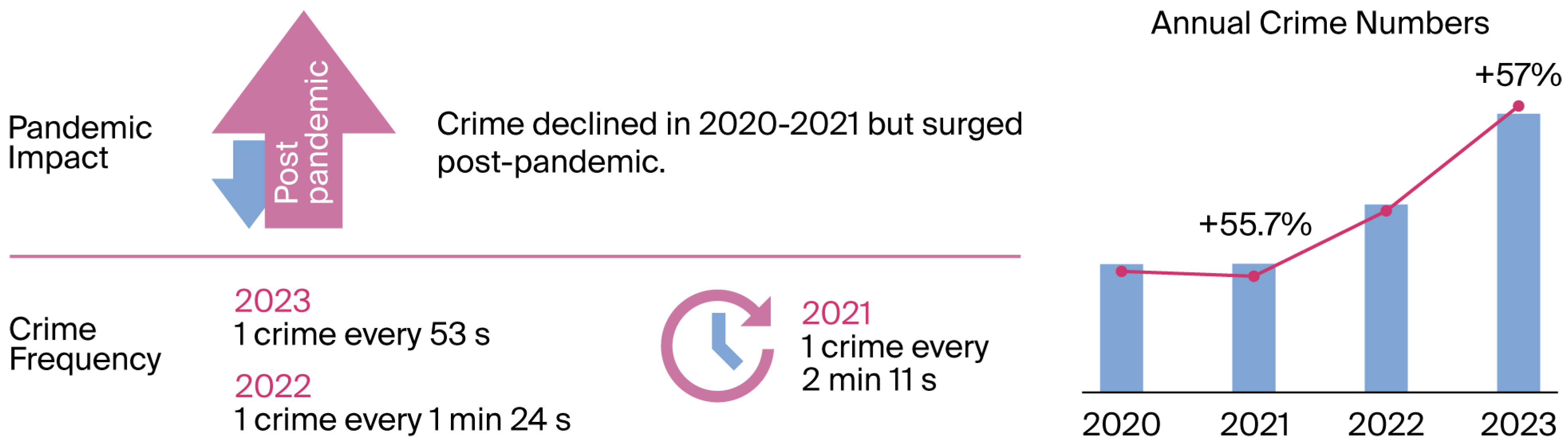
As illustrated in Figure 1, the dramatic post-pandemic crime surge saw incidents escalate from one every 131 s in 2021 to one every 53 s in 2023. Urban centers, particularly on Java Island, experience disproportionately high crime rates due to their population density and economic concentration [1,2,3,4]. The impact of crime extends beyond individual victims, undermining public safety, reducing investment, and creating barriers to national development [5,6].

Traditional crime prevention frameworks are inherently reactive, often limited to post-incident responses rather than proactive intervention. The integration of machine learning and spatio-temporal modeling [7,8] facilitates a paradigm shift toward predictive analytics, leveraging high-dimensional data to anticipate criminal patterns. By harnessing the increasing availability of judicial records, these data-driven approaches offer a mechanism to enhance systemic efficiency, fairness, and resource allocation within legal frameworks [9]. Specifically, XGBoost has demonstrated significant robustness in temporal forecasting [10,11], while the Density-Based Spatial Clustering of Applications with Noise (DBSCAN) provides a specialized capacity for identifying non-linear clusters in large-scale spatial databases [12,13,14]. Despite these global advancements, the application of these integrated methodologies within the unique socio-legal landscape of Indonesia remains significantly under-researched.

1.2. Research Objectives and Problem Statement

This study addresses the need for enhanced crime forecasting in Indonesia by developing a multi-level spatio-temporal machine learning framework using adjudicated crime data from the Supreme Court of Indonesia. While this represents a subset of overall crime occurrences, adjudicated crime data offer distinct advantages, including verified occurrence dates, standardized judicial categorization, and comprehensive geographical coverage across Indonesia’s diverse administrative regions.

The central research problem examines how spatio-temporal machine learning methodologies can enhance adjudicated crime forecasting to support judicial resource planning. This encompasses temporal forecasting model development, spatial crime cluster identification, cross-scale forecasting performance comparison, and the exploration of practical applications for improved crime management.

This study pursues five specific research objectives that collectively advance both the theoretical understanding and practical application of crime forecasting in Indonesia:

• Temporal Forecasting Development: Developing city-level models of adjudicated crime occurrence timelines through the construction and evaluation of XGBoost models for temporal forecasting across individual major Indonesian cities.
• Province-Level Extension: Extending this approach to province-level analysis, creating comparable models that leverage spatio-temporal features and province-level contextual factors.
• Multi-Level Comparative Analysis: Conducting a multi-level comparative analysis of adjudicated crime patterns to identify scale-specific dynamics and assess the relative effectiveness of forecasting at different spatial granularities.
• Spatial Clustering: Employing DBSCAN for spatial clustering to identify statistically significant spatio-temporal clusters across Indonesian major cities and provinces.
• Practical Application Exploration: Exploring practical implications for enhanced crime management strategies through a discussion of potential applications for improving judicial resource planning and regional safety.

2. Related Work

2.1. Criminological Theoretical Foundations

Modern crime forecasting is grounded in established criminological theories that provide essential insights into criminal behavior patterns and spatial-temporal crime dynamics [15].

2.1.1. Routine Activity Theory (RAT)

Routine Activity Theory, developed by Cohen and Felson [16], posits that crime emerges from the convergence of three elements: likely offenders, suitable targets, and the absence of capable guardianship in specific spatio-temporal contexts. Because daily routines exhibit structured spatial-temporal patterns, crime is not randomly distributed but follows predictable, opportunity-driven regularities [17]. This theoretical foundation directly justifies the inclusion of temporal features such as day of week, time of day, and seasonal patterns as core predictors in the forecasting models developed in this study.

2.1.2. Environmental Criminology

Environmental Criminology emphasizes the role of place in crime occurrence, positing that criminal activity clusters spatially due to offender familiarity with locations and the presence of opportunity structures [15,17]. Certain locations become crime generators or attractors due to characteristics such as commercial activity, transportation hubs, or entertainment districts [14,18,19]. This perspective provides the conceptual foundation for the spatial clustering approach employed in this study, explaining why crimes are concentrated geographically rather than distributed randomly across the landscape [20].

2.1.3. Crime Pattern Theory

Crime Pattern Theory further elaborates these concepts through the concepts of “crime generators” and “crime attractors,” which influence the spatial distribution of criminal activity [5,21]. Crime generators are places that attract large numbers of people for legitimate purposes (shopping centers, transit stations), while crime attractors are places that specifically draw motivated offenders (known drug markets, bars). These concepts explain why crimes are concentrated in particular geographical areas and support the use of spatial clustering methods to identify these high-risk locations.

2.1.4. Integrated Theoretical Framework

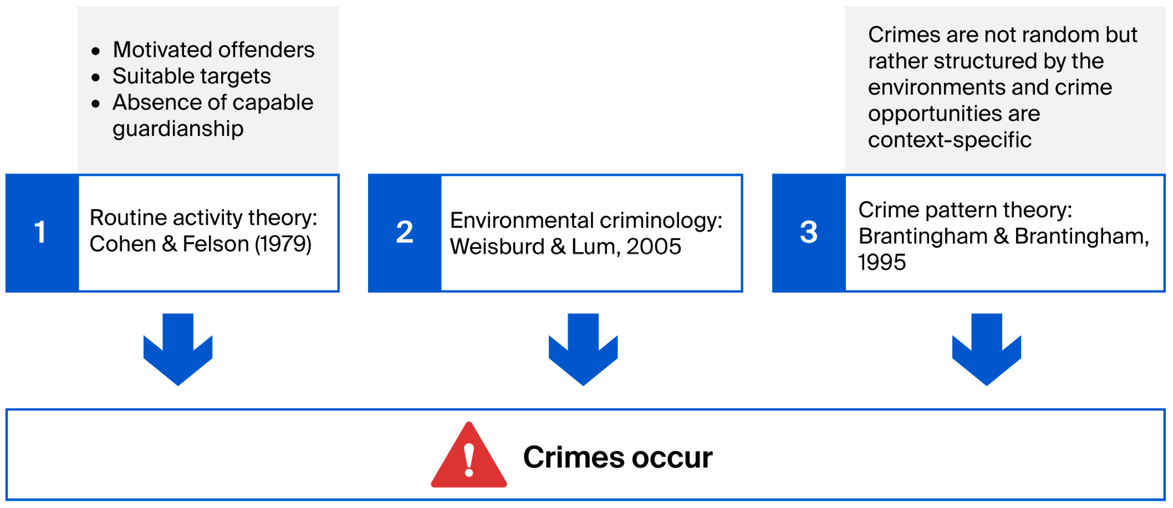
As illustrated in Figure 2, the theoretical framework integrates three key criminological theories: Routine Activity Theory, which focuses on motivated offenders, suitable targets, and the absence of capable guardianship; Environmental Criminology, which examines spatial contexts; and Crime Pattern Theory, which addresses structured environmental influences. These theories converge to explain how crimes occur within specific spatio-temporal contexts, providing a foundation for machine learning approaches to crime forecasting [22]. The integration of these theories justifies the dual-level approach employed in this study, combining temporal forecasting (grounded in RAT) with spatial clustering (grounded in Environmental Criminology and Crime Pattern Theory).

2.2. Machine Learning in Crime Forecasting

2.2.1. Temporal Forecasting Methods

Machine learning applications for crime prediction have evolved significantly over the past two decades, with early efforts employing basic statistical models that exposed persistent challenges such as seasonality, spatial heterogeneity, and near-repeat phenomena [7,23,24,25,26]. Among the methods that emerged, XGBoost has established itself as one of the most effective algorithms for temporal crime forecasting [10,27], with studies reporting impressive R² scores of approximately 76% in predicting hourly crime patterns [10]. Its effectiveness stems from a gradient boosting framework that iteratively builds decision tree ensembles, capturing complex non-linear interactions between temporal and contextual variables while maintaining the computational efficiency required for operational deployment [11].

While LSTM networks excel at capturing long-term sequential dependencies, they typically require large training datasets and are prone to overfitting under data-scarce conditions [28], a significant concern given the 547 daily observations available in this study. They also offer limited interpretability regarding which temporal features drive predictions [20,29]. Prophet, developed by Facebook, performs well on data with clear seasonal patterns through trend–seasonal–holiday decomposition [30,31], but its inherently univariate architecture provides limited support for exogenous features [32], constraining its applicability when multivariate relationships such as population density, GDP, and weather conditions are central to explaining criminal activity patterns.

Given these comparative limitations, XGBoost was selected as the primary temporal forecasting algorithm for this study. Its capacity to handle multi-dimensional feature spaces spanning temporal, contextual, and socioeconomic variables, combined with its robustness to the sparse and noisy data characteristic of crime datasets, its provision of interpretable feature importance rankings, and its consistently superior performance in comparable forecasting studies, make it the most appropriate and operationally viable choice for the research objectives pursued here.

2.2.2. Spatial Clustering Methods

DBSCAN clustering has proven particularly effective for crime hotspot detection due to its ability to identify arbitrarily shaped clusters while handling spatial noise [19]. Unlike K-means, which requires the number of clusters to be specified in advance, DBSCAN automatically determines cluster configurations based on data density, making it well-suited for crime data where hotspot numbers and shapes vary considerably [20]. By identifying core points with sufficient neighboring observations within a defined radius and expanding clusters outward from these points, DBSCAN naturally accommodates the irregular, non-convex spatial geometries that characterize real-world crime hotspots.

DBSCAN offers several advantages for crime analysis. Its ability to identify clusters of arbitrary shape more accurately reflects real-world crime distributions than methods constrained to spherical clusters. Isolated incidents are classified as noise rather than forced into spurious clusters, improving analytical precision. Unlike K-means, DBSCAN requires no pre-specification of cluster numbers, as the algorithm determines groupings automatically based on data density. The method also scales efficiently to large spatial databases, making it suitable for nationwide analysis, and produces clusters that correspond directly to geographically bounded high-density regions, facilitating straightforward practical interpretation.

Recent applications have demonstrated significant improvements in hotspot identification accuracy compared with traditional grid-based approaches [23,33,34,35]. DBSCAN has been successfully applied to crime data in various contexts, including urban crime analysis, gang territory mapping, and resource allocation planning.

2.2.3. Spatio-Temporal Integration

Spatio-temporal modeling integration represents a significant advancement over approaches that treat spatial and temporal dimensions independently. Recent research has explored various approaches, including Deep Spatio-Temporal Graph Attention Networks [36], Space-Time ARIMA (STARIMA) [37], Spatio-Temporal Graph Convolutional Networks (STGCNs) [38], and spatio-temporal cokriging crime prediction using social media data [39]. Systematic literature reviews have identified that ensemble methods and deep learning approaches tend to outperform traditional statistical models, particularly with large-scale, multi-dimensional crime datasets [23]. However, many spatio-temporal approaches require substantial computational resources and large training datasets, making them less practical for developing country contexts with resource constraints.

2.3. Crime Forecasting in Developing Countries

2.3.1. Research Gaps and Contextual Challenges

Despite significant advances in crime forecasting methodologies, several research gaps remain regarding their application in developing countries and archipelagic nations such as Indonesia. Most existing research focuses on developed countries with well-established data collection systems, standardized reporting procedures, and relatively homogeneous urban environments [40]. The unique challenges faced by rapidly urbanizing developing countries require specialized approaches that may not directly translate from the contexts of developed countries [30,41,42].

These challenges manifest across multiple dimensions. Data collection practices vary considerably across jurisdictions and administrative levels, while missing data, inconsistent categorization, and reporting delays further undermine data quality. Limited computing infrastructure and technical expertise constrain the implementation of complex algorithms, and diverse levels of technological adoption across regions compound these difficulties. Additionally, the varied cultural and linguistic contexts that characterize nations like Indonesia influence crime reporting and processing patterns in ways that standard forecasting frameworks are ill-equipped to accommodate.

2.3.2. Adjudicated Crime Data as a Research Opportunity

The existing crime forecasting literature has relied almost exclusively on police-reported incident data, which in developing-country contexts are subject to chronic underreporting, inconsistent categorization, and jurisdictional variation [3,4]. Critically, police-reported statistics serve as a broad indicator of public safety trends, not a reliable predictor of judicial demand, yet this distinction is rarely made explicit in the literature. This study addresses this gap by focusing on adjudicated crime data, comprising cases that have progressed through the full judicial pipeline to a final verdict.

Although adjudicated data represent a filtered subset of overall criminal activity, they offer distinct advantages for the present research context. Having undergone legal verification and sentencing, adjudicated records ensure higher data quality than raw reported statistics. Judicial processes also impose standardized crime categorization through the International Classification of Crime for Statistical Purposes (ICCS), enhancing cross-jurisdictional comparability. Supreme Court records provide comprehensive nationwide coverage, and the inclusion of precise crime occurrence dates makes them directly suitable for temporal forecasting. Most importantly, forecasting adjudicated crime directly supports judicial resource planning and court management, grounding the research in immediate practical relevance that police-reported data cannot provide.

2.3.3. Multi-Level Analysis Approach

This study addresses identified research gaps through a multi-level analysis and the integration of XGBoost temporal forecasting with DBSCAN spatial clustering, providing a methodological framework specifically adapted to Indonesian conditions while maintaining applicability to similar developing country contexts. This study’s focus on adjudicated crime data represents a pragmatic approach to working with available data sources while acknowledging limitations and developing appropriate analytical strategies. The multi-level comparative approach provides insights into the optimal spatial scales for different applications, addressing practical considerations for resource allocation and operational deployment in complex administrative environments.

3. Methodology

3.1. Research Framework

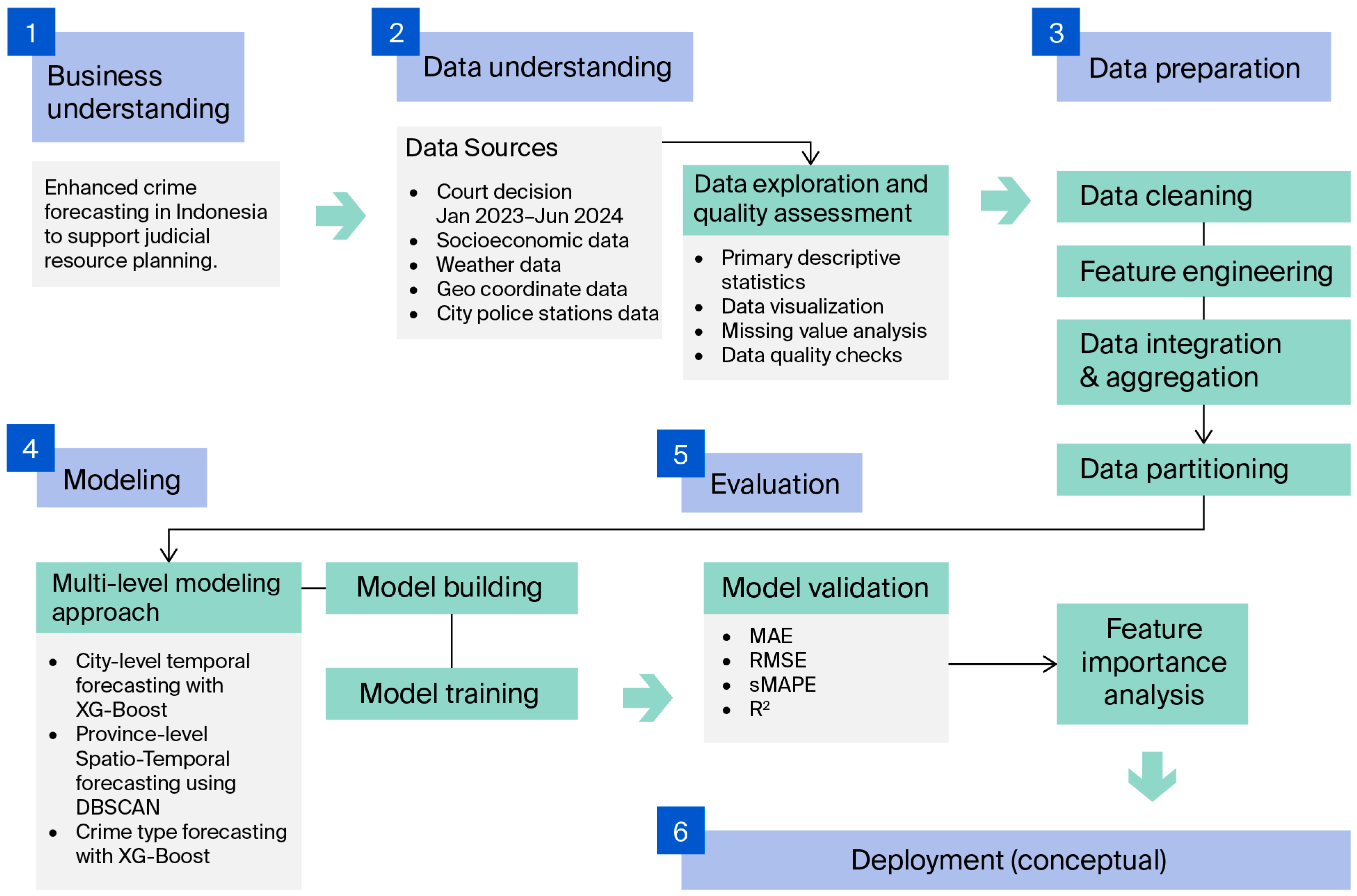
This study employs a comprehensive quantitative methodology following the Cross-Industry Standard Process for Data Mining (CRISP-DM) framework [43]. Despite the emergence of specialized for Big Data methodologies, CRISP-DM remains the most widely adopted process model in both academic research and industrial practice due to its robust, iterative nature [44,45]. This established methodology ensures systematic analysis while maintaining flexibility to address specific challenges associated with crime data analysis. CRISP-DM provides a structured and iterative approach through six phases:

• Business Understanding: Enhanced crime forecasting in Indonesia to support judicial resource planning.
• Data Understanding: Comprehensive analysis of adjudicated crime records from the Supreme Court of Indonesia.
• Data Preparation: Extensive preprocessing, feature engineering, and data cleaning.
• Modeling: Multi-level approaches using XGBoost for temporal forecasting and DBSCAN for spatial clustering.
• Evaluation: Multiple validation metrics and cross-validation strategies.
• Deployment: Conceptual framework for operational implementation.

As illustrated in Figure 3, the methodology follows a systematic approach, beginning with business understanding to enhance crime forecasting in Indonesia. The adoption of this framework allows for a continuous feedback loop, particularly between data preparation and modeling, which is essential when dealing with the high-dimensional nature of criminal records. The data understanding phase involves comprehensive analysis of adjudicated crime records from the Supreme Court of Indonesia. Utilizing adjudicated data rather than raw police reports, this study ensures a higher level of data reliability, as these records have undergone legal verification and sentencing.

3.2. Data Source and Preprocessing

3.2.1. Dataset Description

The primary dataset comprises 95,666 adjudicated crime records sourced from the Supreme Court of Indonesia. The temporal range spans from 1 January 2023 to 30 June 2024, providing a continuous 547-day observation period. Unlike administrative datasets that often rely on court decision dates, this dataset utilizes the actual crime occurrence date, ensuring that the temporal features accurately reflect the timing of criminal activity rather than judicial processing delays. Key variables include the following:

•

Target Variable: Daily crime counts, representing the total frequency of adjudicated offenses across 11 categories (e.g., robbery, assault, drug offenses).

•

Predictive Temporal Indicators: High-resolution time-stamps including Day_of_Week, Month, and binary indicators for Is_Holiday. These support the cyclical encoding process.

•

Spatio-Environmental Covariates: Dynamic daily variables including Average_Temperature and City_Weather. These act as proxies for human mobility and outdoor activity.

•

Static Socioeconomic Context: Cross-sectional variables including City_GDP, Population_Density, and City_Police_Stations. These provide the structural context for the regional crime risk profiles.

•

Demographic Profile: Aggregated characteristics of the offender population, including Offender_Age and Offender_Gender distributions per day.

While the raw data are recorded at the individual case level, the primary unit of analysis for this study is the daily aggregate. The 95,666 individual records were aggregated into a longitudinal series $\left(Y_t\right)$ representing the total daily crime volume. This transformation facilitates the application of structural decomposition and allows for the integration of daily exogenous variables such as local weather patterns and national holidays.

3.2.2. Data Cleaning and Preprocessing

Data preparation followed a rigorous protocol designed to mitigate noise, ensure temporal consistency, and prepare the dataset for residual-based forecasting. The preprocessing phase comprised the following four stages:

• Integrity Verification and Duplicate Suppression: To prevent the artificial inflation of crime frequencies, a multi-stage deduplication process was implemented. Records were filtered based on a unique composite key consisting of the Case_ID and Crime_Date. This ensured that consolidated judicial records representing a single criminal incident were counted as one observation, maintaining the accuracy of the daily aggregate counts.
• Missing Value Imputation and Categorical Cleaning: Initial screening confirmed high data completeness, with missing values confined primarily to specific environmental variables. A targeted imputation protocol was applied: forward-fill was used for time-dependent variables to preserve temporal continuity, while missing socioeconomic and environmental covariates such as GDP, population, and average temperature were resolved through group-wise mean imputation at the city or provincial level, preserving regional variance while generating the continuous data stream required by the XGBoost regressor.
• Statistical Outlier Management: Outliers were identified using a standardized Z-score threshold $\left(\left|Z\right|>3\right)$. In a time-series context, a distinction was made between data entry errors and legitimate “shocks” (e.g., mass public order incidents). While statistical outliers were flagged, they were not automatically removed if they corresponded with documented national events or holidays, as these represented critical “high-variance” signals that the XGBoost model was specifically designed to capture.
• Structural Aggregation and Thresholding: To ensure the statistical power of the predictive models, two primary constraints were implemented. First, individual crime records were aggregated into a daily longitudinal series $\left(Y_t\right)$, a step that serves as a prerequisite for subsequent Augmented Dickey–Fuller (ADF) stationarity testing and STL decomposition. Second, city-level analysis was additionally restricted to jurisdictions with at least 500 adjudicated cases, ensuring sufficient data density for the STL algorithm to reliably separate trend from seasonal components.

3.2.3. ICCS-Based Crime Type Mapping and Standardization

To ensure consistency and comparability across data sources, all crime types were standardized using the International Classification of Crime for Statistical Purposes (ICCS), a framework developed by the United Nations Office on Drugs and Crime (UNODC) [46], as illustrated in

Table 1. ICCS-based crime type mapping.

Local Category	ICCS Mapped Type
Theft, Burglary	Theft
Physical Assault	Assault
Drug Possession	Drug Offenses
Fraud, Forgery	Economic Crimes
Cybercrime	Cybercrime
Homicide	Homicide
Robbery	Robbery
Public Disorder	Public Order
Traffic Violation	Traffic Offense
Sexual Offense	Sexual Crime
Property Damage	Property Crime

. The ICCS provides a hierarchical classification system that enables standardized categorization of crime incidents across jurisdictions and time periods, facilitating international comparisons and evidence-based policy development in criminal justice.

The complete ICCS classification structure and detailed code assignments are documented in the official ICCS Implementation Manual [46]. This standardization framework ensures that crime type definitions remain consistent throughout the analysis and enables comparison with international crime statistics.

Crime type mapping followed the ICCS implementation guidelines [46], adhering to the harmonization methodology principles outlined below:

•

Behavioral Classification: Crime types were classified based on the behavioral characteristics of the offense rather than legal terminology, ensuring consistency with ICCS principles.

•

Hierarchical Structure: The ICCS hierarchical framework was applied to assign crimes to the most appropriate category level.

•

Indonesian Criminal Code Alignment: Mappings were validated against the Indonesian Criminal Code (KUHP) to ensure legal accuracy and national relevance.

•

Documentation: All mapping decisions were documented and are reproducible through reference to the ICCS Implementation Manual.

Adopting this internationally recognized standard enhances the reproducibility and verifiability of the crime type classification scheme employed in this study.

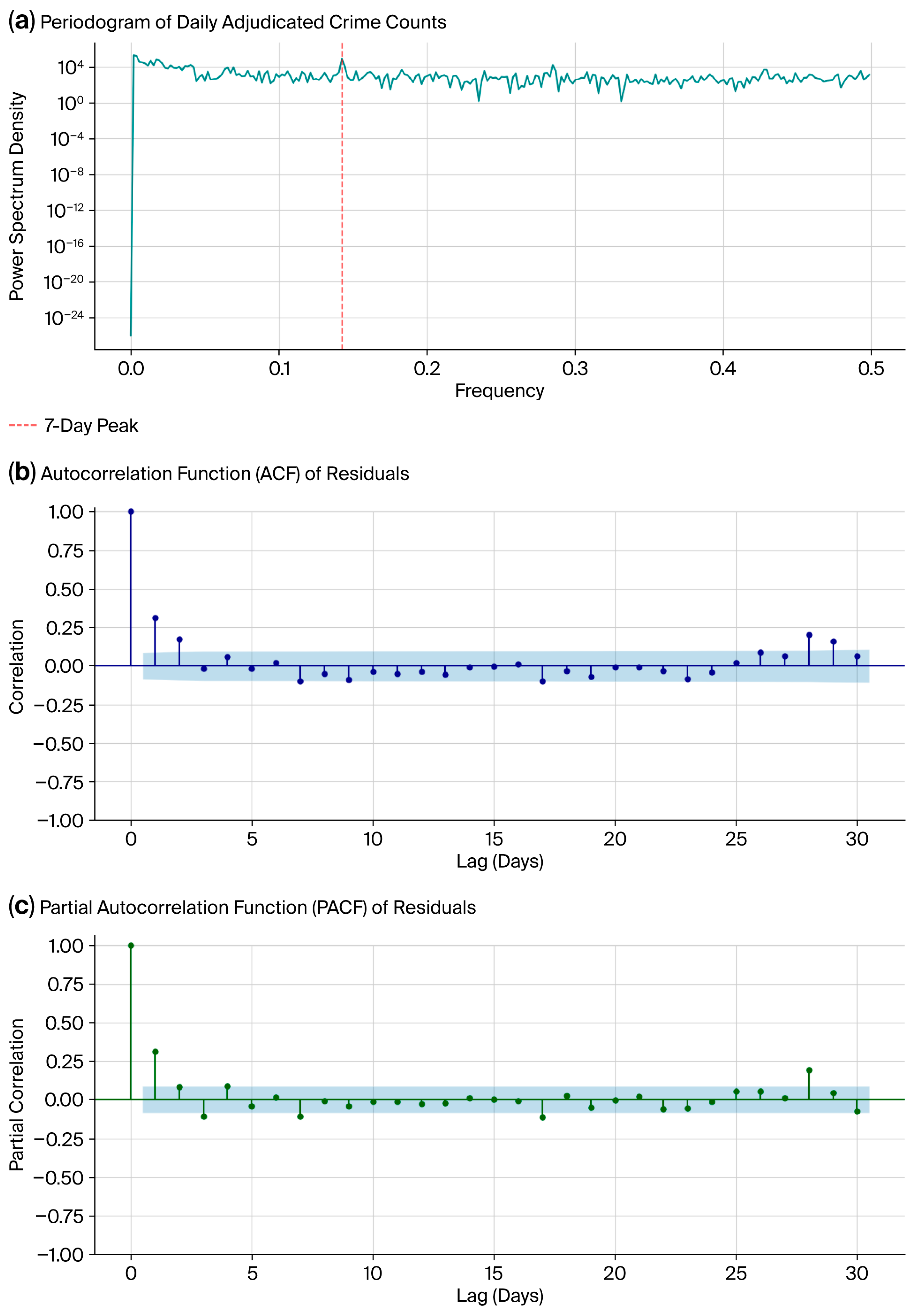
3.2.4. Spectral Analysis via Periodogram

To empirically determine the dominant seasonal cycles within the Indonesian crime series, periodogram (power spectrum) analysis was performed prior to structural decomposition. This method identifies the fundamental frequencies that contribute the most power to the variance of the time series, effectively revealing the hidden rhythms of criminal activity.

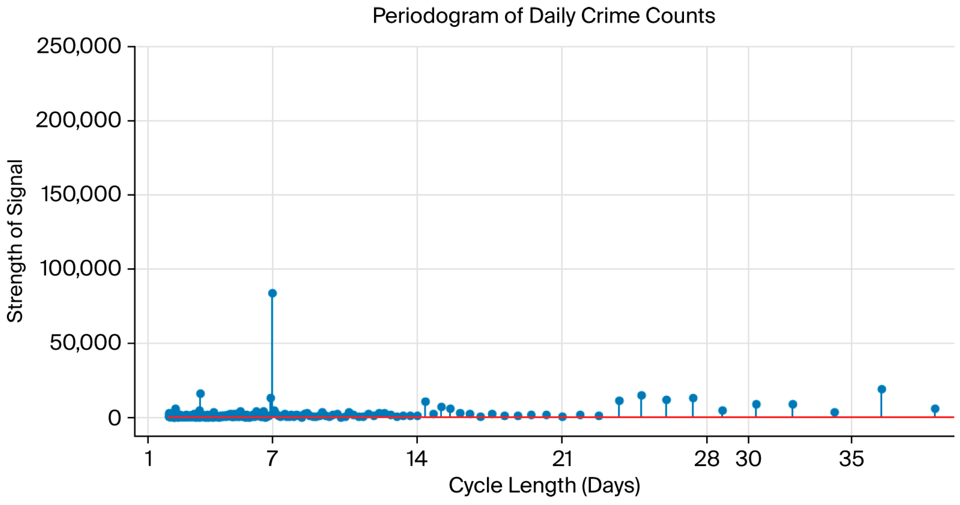
The spectral density revealed two primary peaks of significance. The most dominant peak occurred at the frequency corresponding to the total duration of the dataset (T = 547 days), which represents the global nonstationary trend. Beyond this fundamental frequency, a secondary and highly robust peak was identified at T = 7 days. This identifies a strong weekly seasonality consistent with human social and administrative cycles in urban environments.

The identification of this 7-day cycle provides the statistical basis for the subsequent STL decomposition. By parameterizing the seasonal component at this specific frequency, the hybrid model can effectively isolate the deterministic weekly heartbeat of the city. This allows the XGBoost regressor to focus its predictive power on the stochastic residuals that represent localized shocks and environmental deviations. Figure 4 presents the periodogram results, illustrating the clear dominance of the weekly cycle relative to other potential frequencies.

3.2.5. Feature Engineering

The feature engineering architecture transforms raw nonstationary crime data into a multi-dimensional feature space optimized for residual forecasting. Following the application of STL decomposition to isolate deterministic trend ${(T}_t)$ and seasonal ${(S}_t)$ components, a comprehensive feature vector was constructed. This process incorporates seven distinct categories of variables designed to capture structural signals, high-frequency shocks, local momentum, and exogenous environmental influences, as summarized in

Table 2. Feature categories.

Feature Category	Specific Features	Type	Technical Justification
Structural (STL)	$\mathrm{Trend} \left(T_t\right)$$, \mathrm{Seasonality} \left(S_t\right)$	Numerical	Encodes the low-frequency evolution and latent weekly cycles identified via spectral analysis.
Autoregressive (Lag)	PACF-validated lags (e.g., $t-1,t-7,t-14$)	Numerical	Provides temporal memory; lags are selected based on Partial Autocorrelation Function (PACF) significance.
Cyclical Temporal	$sin/cos$ of Month and Day of Week	Trigonometric	Preserves temporal continuity by mapping time onto a unit circle to avoid chronological boundary gaps.
Dynamic Momentum	7-day Rolling Mean and Std Dev	Numerical	Captures local volatility and short-term density shifts within the residual series.
Exogenous Shocks	Holiday Flag, Avg. Temperature	Binary/ Numerical	Accounts for environmental mobility and significant socio-cultural disruptions to normal patterns.
Socioeconomic	GDP, Population Density, Police Stations	Numerical	Encodes the static risk profile, regional development, and population characteristics of the jurisdiction.
Geospatial	Latitude, Longitude	Numerical	Provides the spatial coordinates necessary for regional clustering and hotspot identification.

.

3.3. Temporal Forecasting with XGBoost

3.3.1. Data Splitting Strategy

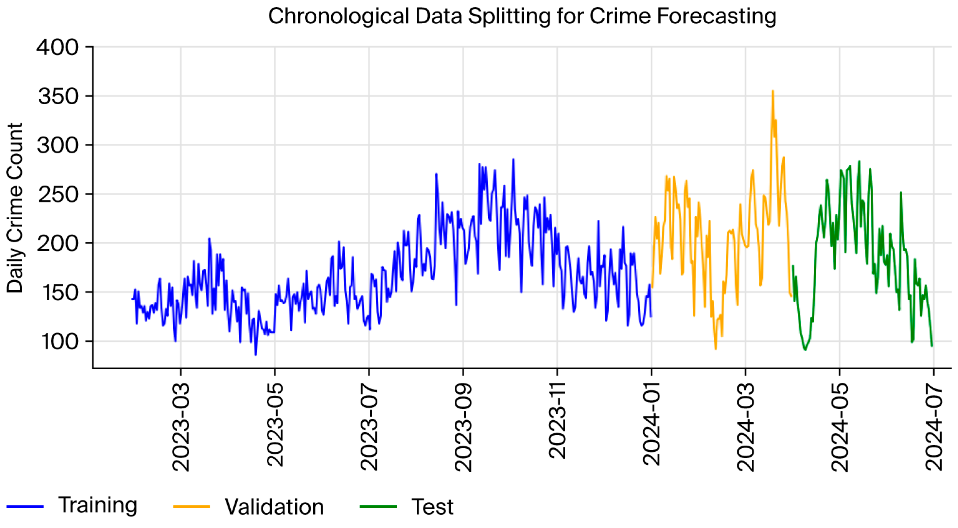
The dataset was partitioned into three distinct temporal periods using a chronological splitting approach. This method preserves the sequential integrity of the crime records and ensures that predictive performance is evaluated on unseen future data. The specific intervals are defined as follows:

•

Training Set: Capturing data from 1 January 2023 to 31 December 2023 (365 days). This period provides the historical baseline for structural decomposition and feature optimization.

•

Validation Set: Capturing data from 1 January 2024 to 31 March 2024 (91 days). This window is used for hyperparameter tuning and monitoring model convergence.

•

Test Set: Capturing data from 1 April 2024 to 30 June 2024 (91 days). This out-of-sample period serves as the final benchmark for assessing the generalization capabilities of the system.

This splitting strategy simulates real-world forecasting scenarios where the model must predict trends beyond its available training history. Figure 5 illustrates the temporal distribution of these splits across the 18-month observation window.

3.3.2. XGBoost Model Development

The forecasting architecture is implemented as a hybrid STL-XGBoost system. This framework follows a multi-stage pipeline designed to handle the inherent non-stationarity of daily crime data.

• Structural Decomposition: The daily aggregate counts are subjected to STL decomposition with a periodicity of $T=7$. This step isolates the deterministic trend and seasonal components, leaving behind the stochastic residuals $\left(R_t\right)$. The methodological goal of this stage is to generate a stationary signal for the machine learning regressor, a process validated through diagnostic testing.
• Autoregressive Feature Identification: To provide the model with temporal memory, the residuals are analyzed using Autocorrelation (ACF) and Partial Autocorrelation (PACF) functions. This allows for the selection of statistically significant lags as autoregressive predictors, ensuring the XGBoost model can capture both immediate and cyclical shocks (the empirical results of this identification process are detailed in Section 4.2).
• Algorithmic Implementation: XGBoost is utilized to predict the isolated residuals. This process includes a GridSearchCV optimization within a TimeSeriesSplit cross-validation framework to identify the optimal hyperparameter configuration while preventing temporal data leakage.

3.3.3. Multi-Level Modeling and Regional Adaptation

The predictive framework was designed to operate across multiple administrative tiers, including national, provincial, and city levels. This hierarchical approach allows for the identification of localized crime dynamics that may be obscured in aggregate data. To ensure the statistical validity of these sub-regional forecasts, two specific adaptation strategies were implemented:

• Data Density Thresholding: City-level models were restricted to jurisdictions demonstrating a minimum volume of 500 adjudicated cases over the 18-month study period. This inclusion threshold serves as a critical quality control measure, ensuring that each resulting time series possesses sufficient information density for the STL algorithm to reliably separate deterministic seasonality from stochastic residuals. In jurisdictions where the case volume fell below this threshold, the signal-to-noise ratio was deemed insufficient for robust evaluation on unseen data.
• Localized Hyperparameter Regularization: Recognizing the variance in data volume across different scales, model hyperparameters were systematically adjusted to prevent overfitting on smaller, more volatile datasets. While national and provincial models utilize higher complexity (e.g., 500 to 1000 estimators), city-level models were configured with increased regularization, including reduced tree depth $\left(max\_depth=3\right)$ and a more conservative number of boosting rounds $\left(n\_estimators=50\right)$. By simplifying the model architecture for localized forecasts, the system maintains high generalization performance even when operating on volatile urban time series.

3.4. Spatial Clustering with DBSCAN

This study moves beyond administrative boundaries to identify organic adjudicated crime hubs using DBSCAN. Unlike traditional centroid-based methods like K-means, DBSCAN is uniquely suited for Indonesian judicial data because it can identify clusters of arbitrary shapes while effectively isolating “noise” (isolated incidents that do not belong to a systemic regional concentration).

3.4.1. Algorithm Overview and Proxy Logic

DBSCAN identifies spatial concentrations based on the density of adjudicated crime incidents in a given geographical area. Due to the unavailability of precise incident-level geographic coordinates in the national judicial record, this study utilizes city centroids (City_Latitude, City_longitude) as spatial proxies. The algorithm classifies data points into three categories:

• Core Points: Cities that have at least a minimum number of neighboring cities ($minPts$) within a specific search radius (epsilon).
• Border Points: Cities that are within the epsilon distance of a core point but do not possess enough neighbors to be core points themselves.
• Noise: Isolated cities that do not belong to any cluster, preventing outliers or rural districts from distorting the results of high-density metropolitan areas.

3.4.2. Parameter Selection and Calibration

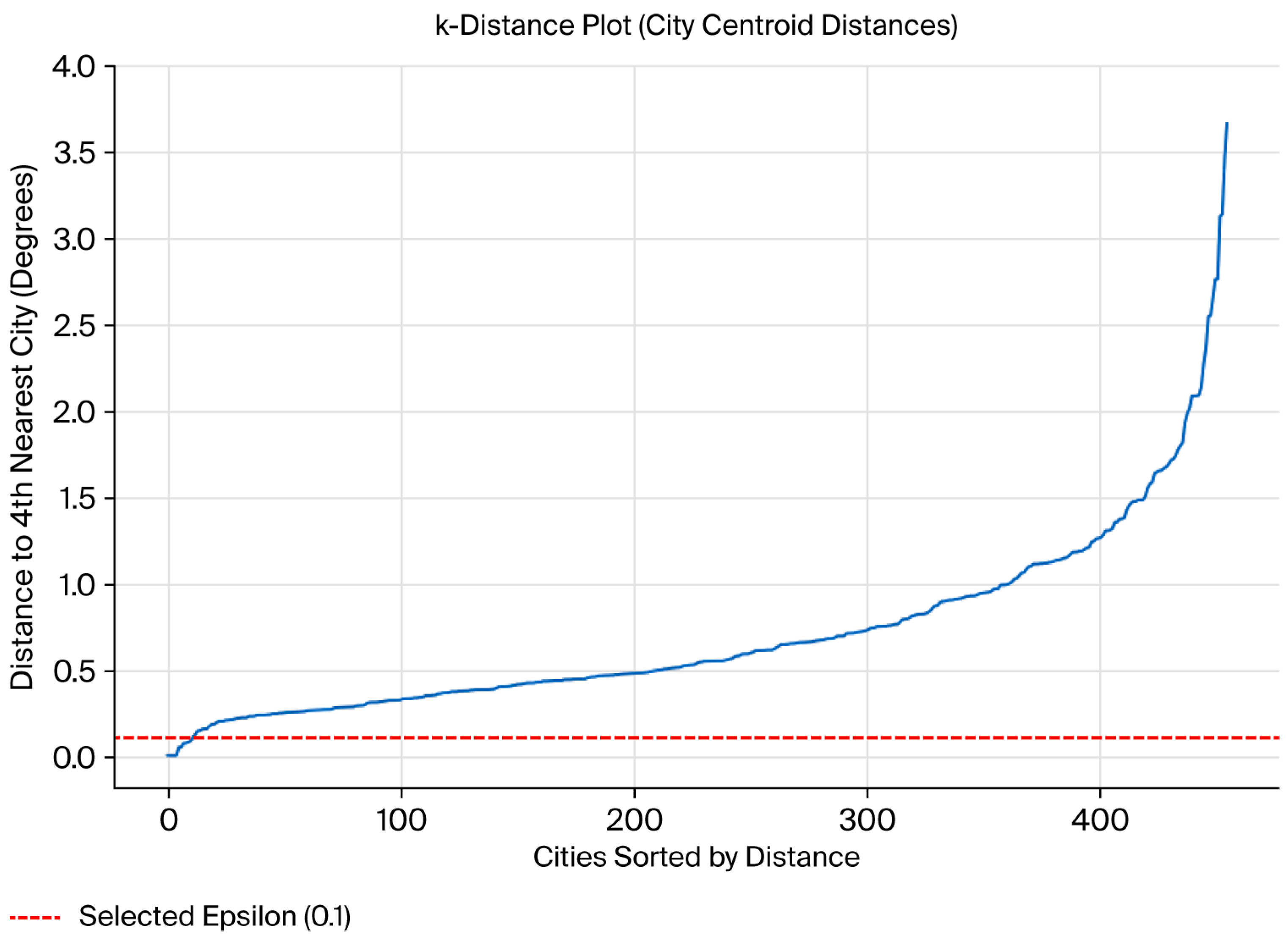
The efficacy of DBSCAN is contingent upon the calibration of two primary parameters: $\mathrm{ϵ}$ (epsilon) and $minPts$. Epsilon $\left(\mathrm{ϵ}\right)$ defines the maximum distance between two city centroids for them to be considered neighbors. To avoid arbitrary selection, the k-distance plot method was employed. By calculating the distance to the $\mathrm{k}$-th nearest neighbor for every city (where $\mathrm{k}=minPts$) and plotting them in ascending order, the “optimal” density threshold is identified at the point of the maximum curvature.

As illustrated in Figure 6, the k-distance distribution exhibits a distinct “elbow” where the curve begins to rise sharply. While initial testing at ${0.1}^{\circ }$ (~11.1 km) identified high-density urban centers, the final model utilized $\mathrm{ϵ}={0.3}^{\circ }$ (~33.3 km). This adjustment ensures the model captures Regional Adjudicated Crime Hubs, such as the connectivity between a major city and its satellite regencies, without over-aggregating geographically separate provincial centers.

The Minimum Points ($minPts$) parameter was set to 3 for the final hub identification. In accordance with density-based clustering theory, $minPts$ must be at least $\mathrm{d}\mathrm{i}\mathrm{m}+1$. Given the use of city centroids as proxies, a value of 3 ensures that a geographical area is only recognized as an adjudicated crime hub if it represents a functional ecosystem of at least three neighboring jurisdictions, thereby prioritizing systemic regional patterns over isolated municipal activity.

All analyses were conducted utilizing the WGS 84 (EPSG:4326) geographic coordinate system, with distances computed using the Haversine formula to accurately account for the curvature of the Earth across the dispersed geography of the Indonesian archipelago.

3.4.3. Sensitivity Analysis and Validation

To ensure the spatial integrity of the identified adjudicated crime hubs, a sensitivity analysis was performed across a parameter grid $\left(\mathrm{ϵ}\in \left[0.1,0.3,0.5\right];minPts\in \left[3,5,10\right]\right)$. The stability of the clustering configuration was validated using the Pairwise Jaccard Similarity Index, which measures the consistency of city-to-cluster assignments relative to the optimized baseline.

The Pairwise Jaccard Index $\left(J\right)$ for two clustering results, $A$ and $B$, is defined as

$$J\left(A,B\right)={\displaystyle \frac{\left|S_A\cap S_B\right|}{\left|S_A\cup S_B\right|}}$$

where ${\mathrm{S}}_{\mathrm{A}}$ is the set of pairs of cities $\left(i,j\right)$ that belong to the same cluster in configuration $A$. A value of 1.0 indicates perfect stability, while a value approaching 0.0 suggests that the hubs are highly sensitive to minor parameter shifts.

As shown in

Table 3. DBSCAN sensitivity analysis and cluster stability results.

$\mathbf{Epsilon} \left(\mathsf{ϵ}\right)$	minPts	Number of Hubs	Jaccard Index	Stability Interpretation
0.1	3	7	0.0862	Fragmentation (Over-constrained)
0.1	5	2	0.0650	Data Sparsity
0.1	10	0	0.0000	Null Results
0.3 (Base)	3	29	1.0000	Optimal Configuration
0.3	5	10	0.4054	Loss of Regional Connectivity
0.3	10	1	0.1102	High Attrition
0.5	3	28	0.1778	Geographic Bleeding
0.5	5	17	0.2271	Moderate Aggregation
0.5	10	2	0.3258	Structural Collapse

, the stability analysis results for the spatial radius $\left(\mathrm{ϵ}\right)$ reveal that a restrictive radius of $\mathrm{ϵ}=0.1\left(\sim 11 \mathrm{k}\mathrm{m}\right)$ resulted in a dramatic collapse of the Jaccard Index (0.0862), identifying only 7 hubs. This suggests that judicial activity in Indonesia is organized across broader regional corridors that exceed a strictly local radius. Conversely, expanding the radius to $\mathrm{ϵ}=0.5$ led to a significant drop in stability (0.1778), as distinct regional hubs began to merge into spatially over-aggregated macro-clusters, thereby obscuring the localized categorical crime typologies identified in Section 4.1.3.

For the impact of density thresholds ($minPts$), the analysis reveals that the Indonesian adjudicated landscape is characterized by small, high-intensity jurisdictional clusters. Increasing the $minPts$ requirement from 3 to 10 led to the disappearance of 96.5% of the clusters $\left(29\to 1\right)$ and a low stability score of 0.1102. This confirms that the most significant judicial activity occurs in “triangulated” jurisdictions (e.g., three neighboring regencies/cities), justifying the use of $minPts=3$ to capture these critical regional linkages.

Therefore, based on the results in Table 3, the configuration of $\mathrm{ϵ}=0.3$ and $minPts=3$ was selected as the study’s baseline. This combination maximizes the Jaccard stability while preserving the granularity required to distinguish between separate metropolitan clusters, providing a robust foundation for the subsequent spatio-temporal forecasting models.

3.5. Evaluation Metrics

Model evaluation employs a multi-faceted approach to quantify predictive accuracy, utilizing Mean Absolute Error (MAE), Root Mean Square Error (RMSE), Symmetric Mean Absolute Percentage Error (sMAPE), and the Coefficient of Determination $\left({\mathrm{R}}^2\right)$. Temporal validation was conducted using time-series cross-validation to maintain chronological integrity and prevent data leakage.

MAE measures the average magnitude of errors in a set of predictions without considering their direction. It represents the average absolute difference between the predicted values and actual observations, where all individual differences are weighted equally.

$$\mathrm{M}\mathrm{A}\mathrm{E}={\displaystyle \frac{1}{n}}\sum _{i=1}^n\left|y_i-\widehat{y_i}\right|$$

RMSE is a quadratic scoring rule that measures the average magnitude of error. By squaring the differences before averaging, RMSE assigns a higher penalty to large errors or outliers. This is particularly useful in crime forecasting for identifying models that fail significantly during extreme crime spikes.

$$\mathrm{R}\mathrm{M}\mathrm{S}\mathrm{E}=\sqrt{{\displaystyle \frac{1}{n}}\sum _{i=1}^n{\left(y_i-\widehat{y_i}\right)}^2}$$

While standard MAPE is commonly used for forecast evaluation, it exhibits numerical instability and upward bias when actual values approach zero, a frequent occurrence in daily crime data during weekends. Symmetric MAPE (sMAPE) was adopted instead, as its symmetric formulation bounds the error range and eliminates division-by-zero risk, providing a more reliable percentage-based accuracy metric for volatile time-series data.

$$\mathrm{s}\mathrm{M}\mathrm{A}\mathrm{P}\mathrm{E}={\displaystyle \frac{100\mathrm{\%}}{n}}\sum _{i=1}^n\left|{\displaystyle \frac{y_i-\widehat{y_i}}{{\left(\right|y}_i\left|+\left|\widehat{y_i}\right|\right)/2}}\right|$$

The ${\mathrm{R}}^2$ score represents the proportion of variance in the dependent variable that is predictable from the independent variables. In the context of this research, ${\mathrm{R}}^2$ is critical for assessing how well the hybrid model captures the underlying temporal patterns and the “fit” of the adjudicated crime fluctuations rather than merely predicting the mean.

$$R^2=1-{\displaystyle \frac{\sum {\left(y_i-\widehat{y_i}\right)}^2}{\sum {\left(y_i-\overline{y}\right)}^2}}$$

3.6. Computational Environment and Instrumentation

The machine learning framework and spatial analyses were executed on a standard cloud virtual machine (specifically an n2-standard-16 instance) featuring 16 vCPUs and 64 GB of RAM. This infrastructure was provisioned via the Google Cloud Platform (Compute Engine; Google LLC, Mountain View, CA, USA). The software environment was built on Windows 11 Pro v. 25H2 (Microsoft Corp., Redmond, WA, USA) utilizing Jupyter Notebook v. 7.0.6 and Python v. 3.12. Core analytical libraries included XGBoost v. 3.2.0 (DMLC, Open Source) for temporal forecasting, Scikit-learn v. 1.3.2 (Inria, Paris, France) for DBSCAN clustering, and Statsmodels v. 0.14.1 (Open Source) for STL decomposition.

4. Result

4.1. Adjudicated Crime Trends and Temporal Analysis

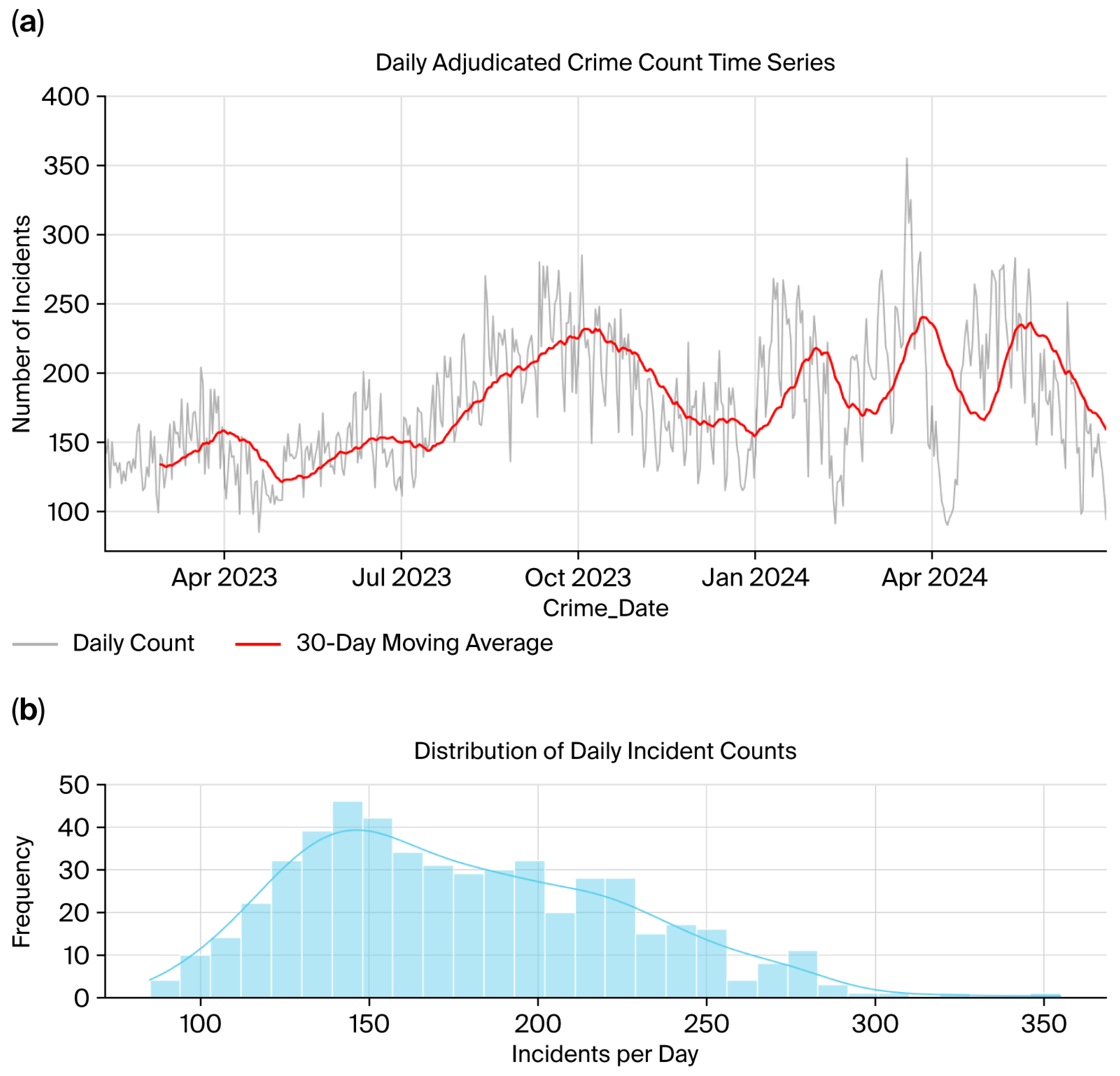
Analysis of 95,666 adjudicated crime records spanning 18 months, from 1 January 2023 to 30 June 2024, reveals the temporal dynamics underlying the crime series and empirical foundation necessary for robust predictive forecasting. Daily crime counts averaged 174.89 incidents with a standard deviation of 46.99, reflecting the coexistence of systematic patterns and stochastic fluctuations. A consistent weekly cycle emerged throughout the observation period, with weekdays recording markedly higher counts than weekends, a pattern consistent with Routine Activity Theory, which attributes such regularities to the structured rhythms of population mobility and commercial activity [16].

As shown in Figure 7a, the daily time series exhibits persistent high-frequency fluctuations that reflect both genuine variations in criminal activity and the inherent noise present in administrative court records. The 30-day moving average, represented by the red line, indicates that while localized upward and downward shifts in crime volume occur across distinct sub-periods, the overall baseline remains relatively stable and centered around 175 cases per day, suggesting the absence of a strong long-term upward or downward trend within the observation window. Figure 7b displays the statistical distribution of daily incident counts, confirming that the majority of days fall within the 120 to 220 case range. The distribution exhibits a slight right-skew, reflecting the occurrence of episodic peak crime days that temporarily elevate volume beyond the typical range, likely associated with specific judicial processing cycles or external socioeconomic events.

To justify the hybrid modeling approach, stationarity diagnostics were conducted. The raw daily aggregate series was analyzed using the Augmented Dickey–Fuller (ADF) test, yielding a statistic of $-3.60 \left(p<0.01\right)$. Although stationary, the series contains a deterministic weekly cycle. Following the application of STL decomposition, the isolated residuals achieved a significantly higher degree of stationarity (ADF Statistic: $-8.98,p<0.0001)$. This indicates that removing the seasonal and trend components creates a refined stochastic signal for the XGBoost regressor.

4.1.1. Weekly Pattern Analysis

The investigation into temporal rhythms within the adjudicated crime dataset reveals a consistent and statistically robust weekly cycle that characterizes crime occurrences reaching final adjudication in Indonesia. Statistical analysis of daily incident volumes across the full 18-month observation period confirms that criminal activity is not uniformly distributed across the days of the week but instead follows a structured and recurring pattern. As presented in

Table 4. Weekly crime pattern analysis.

Day of the Week	Mean Incidents	Percentage of Weekly Average (%)	Standard Deviation	Sample Size (Days)
Monday	189.28	106.92	48.63	74
Tuesday	189.62	107.11	52.06	74
Wednesday	191.26	108.04	48.85	74
Thursday	183.26	103.52	48.19	74
Friday	177.41	100.21	43.56	74
Saturday	160.41	90.61	35.96	74
Sunday	148.37	83.81	33.51	75

, a clear peak in judicial caseload volume occurs during the midweek period, specifically between Tuesday and Thursday, after which incident counts progressively decline toward the weekend. This concentration of cases in the middle of the working week likely reflects the compound influence of institutional scheduling practices within the Indonesian judicial system, including court session calendars, police reporting cycles, and prosecutorial processing timelines, all of which tend to converge during core business days.

This weekly pattern demonstrates that midweek periods experience peak counts, while weekends (Saturday and Sunday) show significantly reduced activity. Sunday recorded the minimum average, at approximately 51% of the overall weekly daily mean. This pattern aligns with Routine Activity Theory, suggesting that weekday commercial and social activities create more crime opportunities than weekend patterns [16]. Furthermore, this reduction reflects the operational schedules of the judicial system and the decrease in formal legal proceedings during weekends. This concentration of adjudicated cases during the working week suggests that the temporal distribution is influenced by both social routines and the structured activities of legal institutions. These findings provide the empirical basis for selecting a seven-day periodicity $\left(\mathrm{T}=7\right)$ for the subsequent STL decomposition, ensuring that the weekly seasonal component is accurately isolated from the underlying trend.

4.1.2. Temporal Structure Analysis

To quantify periodicities within the crime time series, spectral analysis and autocorrelation diagnostics were performed. As shown in Figure 8a, the periodogram reveals a sharp spectral peak at the frequency corresponding to a seven-day cycle, confirming weekly seasonality as the dominant rhythmic structure governing adjudicated crime counts.

Following the removal of deterministic components via STL decomposition, the resulting residual series was further analyzed for autoregressive properties. The Autocorrelation Function (Figure 8b) displays significant spikes at weekly intervals, suggesting that seasonal dependencies persist within the broader stochastic signal even after trend and seasonal extraction. More critically, the Partial Autocorrelation Function (Figure 8c) identifies statistically significant spikes at Lag 1 and Lag 28. These findings indicate that the most recent daily observation and the observation from the previous four-week cycle together provide the strongest predictive information for the XGBoost regressor. Consequently, both of these lag values were deliberately incorporated as core engineered features in the final model development pipeline, ensuring that the model could explicitly capture both immediate recency effects and longer-range monthly periodicity.

The collective identification of these temporal dependencies across multiple diagnostic tools confirms that the adjudicated crime series is jointly composed of deterministic cyclical patterns and stochastic shocks that operate at different timescales. This composite structure necessitates a formal and systematic decomposition procedure to isolate and separate these components prior to model training, ensuring that the predictive model is trained on a stationary and well-characterized signal rather than a confounded mixture of trend, seasonality, and noise.

4.1.3. Geographical Distribution of Crime Categories

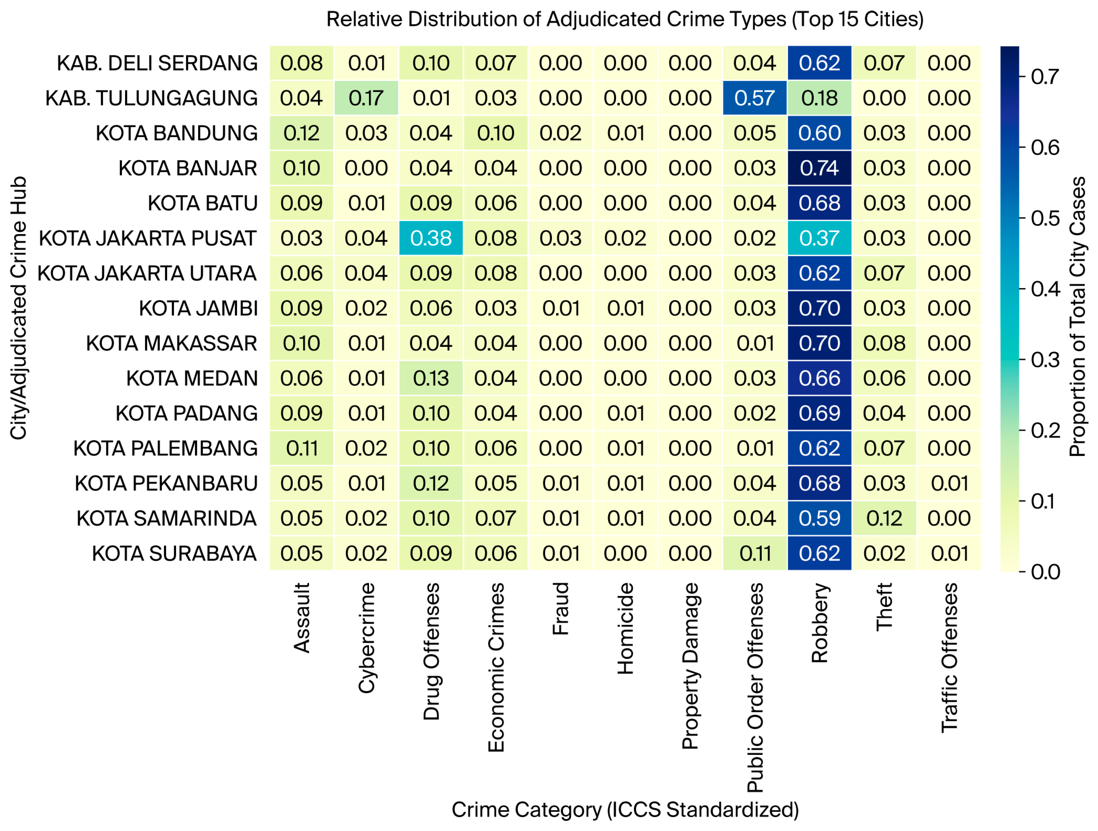
To identify regional variations in the nature of crimes reaching final adjudication, a cross-tabulation of crime types across the fifteen highest-volume jurisdictions was systematically conducted. As illustrated in Figure 9, the composition of legal caseloads is not uniform across the archipelago, with each jurisdiction exhibiting a distinctive distribution of crime categories that reflects the underlying socioeconomic, geographic, and demographic characteristics of its respective region.

The heatmap in Figure 9 reveals that narcotics-related offenses represent a systemic baseline across all major hubs, particularly in Medan and Surabaya. However, property-related crimes and fraud exhibit significantly higher density in the Jakarta Core Hub, suggesting a correlation between urban financial centers and specific judicial caseloads. These categorical disparities justify the “Multi-level Modeling” approach defined in Section 3, as the temporal drivers for narcotics may differ substantially from those of property crime.

4.1.4. Comparative Analysis: The Judicial Funnel (BPS vs. Adjudicated Data)

To validate this study’s dataset against national benchmarks, a comparative analysis was conducted between the adjudicated incidents and the official reported crime statistics for the 2023 calendar year [3]. This analysis identifies the “Judicial Funnel,” the structural attrition that occurs as criminal incidents move through the police, prosecutorial, and judicial filters.

To ensure a rigorous comparison, the following data integration framework was applied:

•

Reported Crime Source: Official national crime statistics provided by the Indonesian Statistical Bureau (BPS).

•

Adjudicated Crime Source: Judicial records sourced from the Supreme Court of Indonesia.

•

Harmonization Rules: Crime categories were mapped using the ICCS. Minor discrepancies in definitions between police reporting and judicial sentencing were resolved by assigning cases to the most similar ICCS category to maintain statistical consistency.

•

Metric Calculation: The attrition gap (%) was calculated as

$$Gap=\left({\displaystyle \frac{Reported-Adjudicated}{Adjudicated}}\right)\times 100$$

and the adjudication rate (%) represents the percentage of reported cases reaching finality:

$$Rate=\left({\displaystyle \frac{Adjudicated}{Reported}}\right)\times 100$$

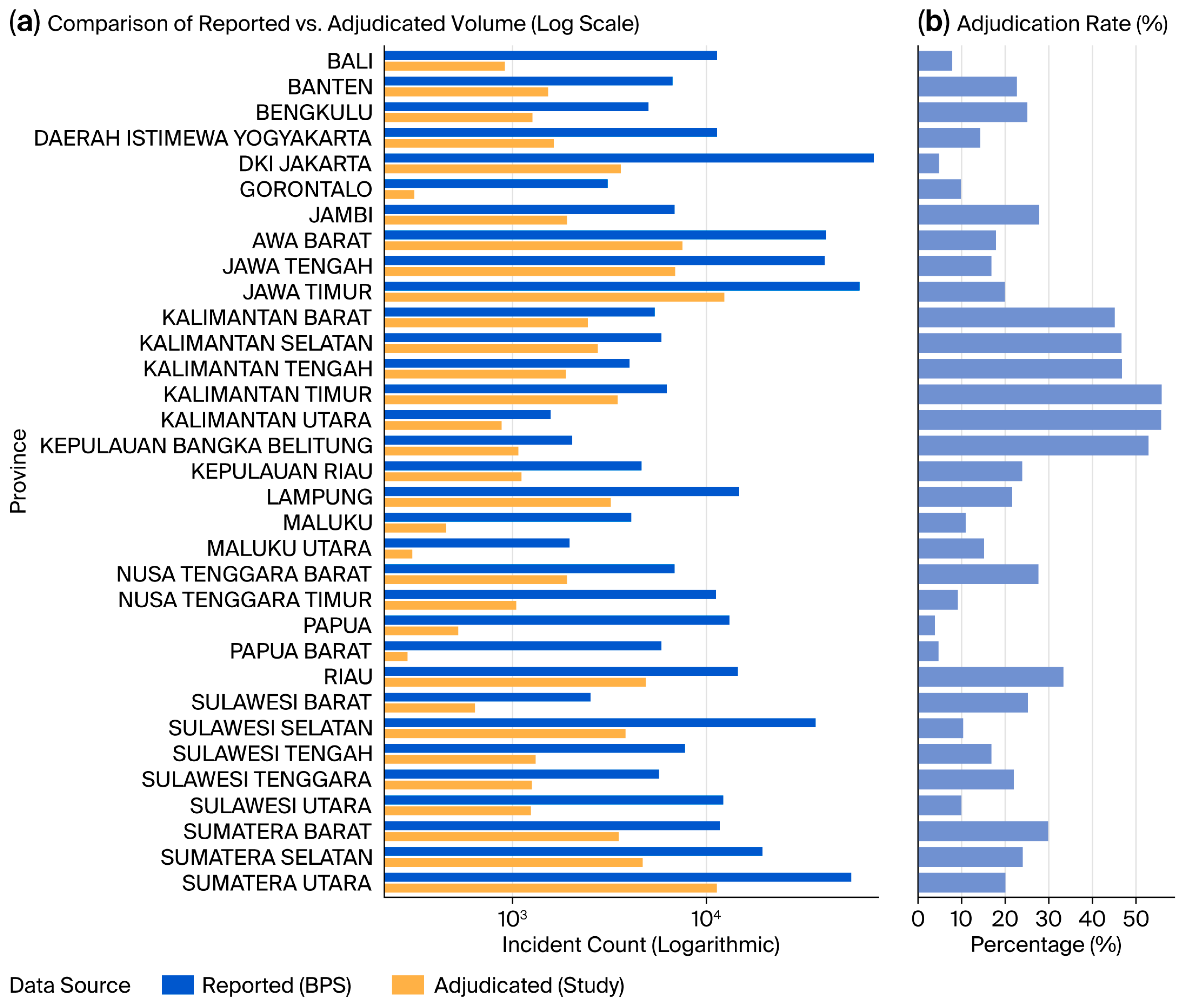
As illustrated in Figure 10, the disparity between reported crime and final legal outcomes reveals significant regional variations in judicial processing. These quantitative relationships are further detailed in

Table 5. The judicial funnel: reported vs. adjudicated crime volume (top 10 provinces).

Province	Reported (BPS)	Adjudicated	Adj. Rate (%)	Gap (%)
DKI Jakarta	73,934	3627	4.91%	1938.43
Jawa Timur	62,272	12,456	20.00%	399.94
Sumatera Utara	56,542	11,361	20.09%	397.68
Jawa Barat	42,018	7543	17.95%	457.05
Jawa Tengah	41,004	6922	16.88%	492.37
Sulawesi Selatan	36,957	3834	10.37%	863.93
Sumatera Selatan	19,552	4692	24.00%	316.71
Lampung	14,818	3216	21.70%	360.76
Riau	14,645	4896	33.43%	199.12
Papua	13,238	522	3.94%	2436.02

.

Extreme Attrition in Metropolitan and Remote Jurisdictions. The data reveal that Papua (3.94%) and DKI Jakarta (4.91%) exhibit the narrowest judicial funnels in the country. In Jakarta, the extreme attrition gap (1938.43%) suggests a high volume of “street-level” reports that are resolved via administrative fines or restorative justice (RJ) mechanisms without reaching formal adjudication. In Papua, the gap (2436.02%) likely reflects logistical and geographical constraints in the formal transfer of cases from police to the judiciary, a common challenge in dispersed archipelagic regions.

Regional Adjudication Efficiency and Cluster Stability. Conversely, Riau (33.43%) and Sumatera Selatan (24.00%) demonstrate significantly higher adjudication rates. This indicates a “wider” funnel, where a larger proportion of reported incidents successfully navigate the evidentiary and prosecutorial hurdles required for a final verdict. For the spatial clustering models (Section 4.6), these provinces provide a high-fidelity signal, as the link between a reported event and a judicial outcome is most direct.

Implications for Forecasting and Judicial Policy. Critically, these results imply that the forecasting models developed in this study (STL-XGBoost) should be interpreted as predictors of judicial workload and legal finality rather than a comprehensive census of social deviance. While BPS data provide a broader view of public safety concerns, adjudicated data provide a direct predictive indicator of court congestion and prosecutorial demand. This distinction is vital for judicial administrators seeking to optimize resource allocation and digital evidence management within emerging data-driven justice frameworks.

4.2. Structural Decomposition Results

Following the identification of the temporal structure, the aggregate crime series was decomposed using Seasonal-Trend decomposition via LOESS (STL). This phase represents the transition from data exploration to model implementation, isolating the deterministic components to reveal the underlying stochastic residuals.

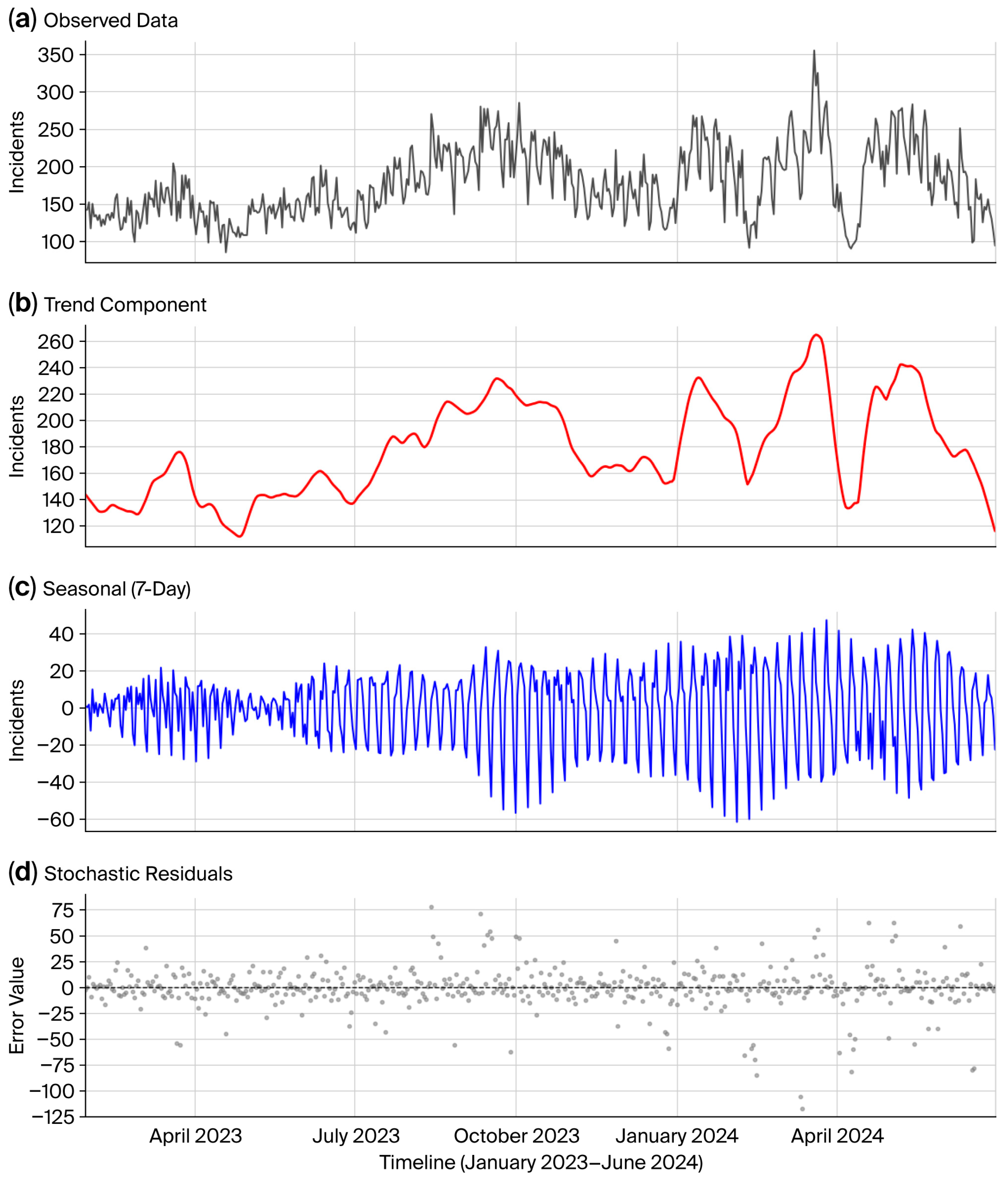
STL decomposition successfully partitioned the crime counts into trend, seasonal, and residual components. As illustrated in Figure 11, the seasonal component (Panel c) exhibits a rigid and stable seven-day oscillation that accounts for the primary periodic variance identified in the earlier spectral analysis. The trend component (Panel b) captures localized shifts in the baseline adjudicated crime volume, which remains relatively stable but displays subtle low-frequency movements throughout the study period.

The extraction of residual components (Panel d) is the pivotal output for the subsequent machine learning phase. These residuals reflect the irregular shocks and deviations from the expected seasonal and trend patterns. While the raw crime data exhibited stationarity, the removal of the deterministic cycles significantly improved the signal quality for the XGBoost regressor. The resulting residual series achieved an ADF statistic of −8.98 $\left(p<0.0001\right)$, confirming that the data were successfully transformed into a highly stationary state optimized for forecasting.

4.3. Model Performance and Evaluation

To evaluate the predictive accuracy of the hybrid STL-XGBoost model, several key performance indicators were utilized. The model was assessed using MAE, RMSE, the Coefficient of Determination $\left(R^2\right)$, and Symmetric MAPE. These metrics provide a comprehensive overview of the model’s ability to handle both the magnitude of crime incidents and underlying variance of the stochastic residuals.

4.3.1. Impact of Hyperparameter Optimization

To quantify the technical rigor of the modeling process, a comparative analysis was conducted between the base XGBoost configuration and optimized version. The base model, utilizing initial parameters, provided a robust baseline with an $R^2$ score of 0.7412. However, the subsequent application of GridSearchCV to optimize the learning rates, tree depth, and subsampling ratios resulted in a measurable enhancement of the model’s explanatory power.

As detailed in

Table 6. Comparative model performance: base vs. optimized results.

Metric	Base Model	Optimized (Final)	Improvement (%)
Mean Absolute Error (MAE)	16.7200	16.5200	1.20
Root Mean Squared Error (RMSE)	23.1700	23.1000	0.30
sMAPE (%)	10.6100	9.7600	8.01
R-squared (R2) Score	0.7412	0.8070	8.88

, the optimized model (learning_rate = 0.01, max_depth = 5, n_estimators = 500) achieved a final R² score of 0.8070, representing an 8.88% improvement of R² score in capturing daily variance. While the reduction in absolute error (MAE) was 1.20%, the significant drop in sMAPE to 9.76% (an 8.01% improvement) confirms that the tuning process specifically refined the model’s sensitivity to high-frequency fluctuations and periodic crime spikes. These results suggest that the hybrid approach is highly reliable, maintaining an average percentage error below the 10% threshold despite the inherent volatility of the adjudicated crime data.

4.3.2. Predictive Accuracy Visualization

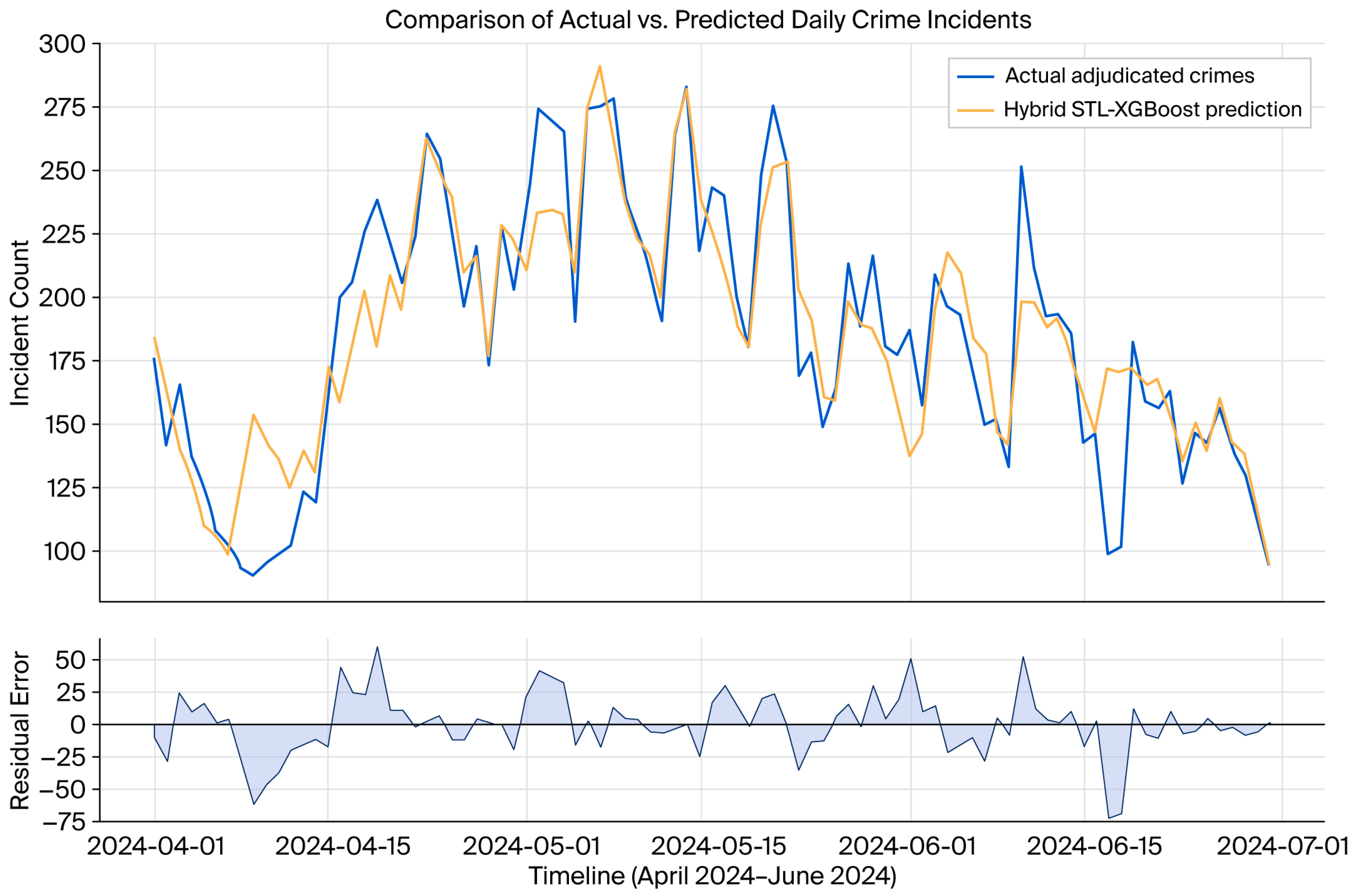
To visually assess the model’s performance, the reconstructed predictions were plotted against the actual adjudicated crime counts for the test period (1 April 2024 to 30 June 2024). As illustrated in Figure 12, the hybrid STL-XGBoost model exhibits a high degree of synchronization with the ground truth data.

The visualization confirms that the model accurately captures the recurrent seven-day seasonality, successfully identifying the midweek peaks and weekend troughs that characterize the Indonesian judicial cycle. Notably, the model also demonstrates the ability to anticipate stochastic spikes in crime volume, which are represented by the residuals predicted by the XGBoost component. The tight alignment between the two series, particularly during the transition from high- to lower-activity weekends, visually validates the high $R^2$ score and low sMAPE reported in Section 4.3.1.

4.4. Feature Importance Analysis

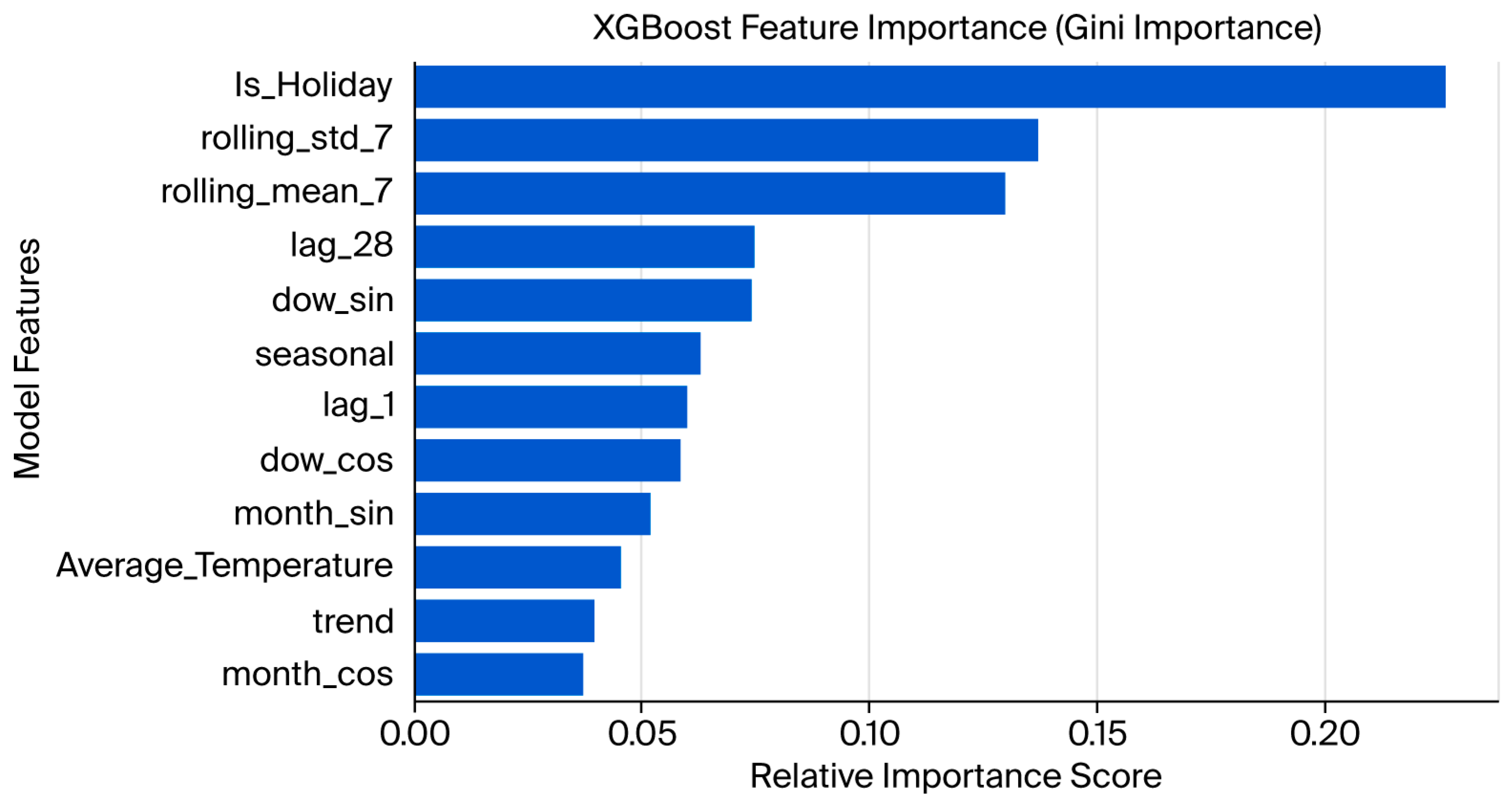
To interpret the internal decision-making process of the optimized hybrid model, a feature importance analysis was conducted using the Gini Importance metric. This provides transparency into which variables contribute the most to reducing the variance of the stochastic residuals. As presented in

Table 7. XGBoost feature importance scores (optimized model).

Feature	Importance Score
Is-Holiday	0.2268
rolling-std-7	0.1374
rolling-mean-7	0.1300
lag-28	0.0748
Day-of-Week (Sine)	0.0741
STL-Seasonal	0.0630
lag-1	0.0602
Day-of-Week (Cosine)	0.0587
Month (Sine)	0.0521
Average-Temperature	0.0456
STL-Trend	0.0399
Month (Cosine)	0.0374

and Figure 13, the model’s predictive intelligence is driven by a combination of exogenous shocks, recent volatility, and deep temporal memory.

4.5. Multi-Level Spatial Performance Analysis

To assess the scalability of the hybrid STL-XGBoost model, the analysis was disaggregated into provincial and city-level time series. This multi-level approach identifies the spatial granularities at which temporal forecasting remains a viable tool for judicial resource planning.

4.5.1. Province-Level Extension

The model was extended to the provincial level to account for regional administrative variations. As presented in

Table 8. Province-level performance (top 5 by R²).

Location	Level	MAE	sMAPE (%)	R2	Samples
Jawa Tengah	Province	3.27	25.92	0.6647	6922
Jawa Timur	Province	4.80	21.02	0.6399	12,456
Sumatera Utara	Province	3.89	17.87	0.6279	11,361
Sulawesi Tenggara	Province	0.89	69.70	0.5639	1257
Sulawesi Tengah	Province	0.84	78.40	0.5500	1315

, the model demonstrated its highest reliability in high-volume provinces. Jawa Tengah and Jawa Timur emerged as the top performers, with $R^2$ scores of 0.6647 and 0.6399, respectively.

The successful mapping in these regions is attributed to the substantial sample sizes (e.g., n = 12,456 for Jawa Timur), which provide a clear enough signal for the XGBoost regressor to map the relationship between national holidays and local crime residuals. The sMAPE values, though higher than the national aggregate, remain stable between 17% and 26% for the top three provinces, satisfying the requirements for strategic regional oversight.

4.5.2. City-Level Temporal Forecasting

At the municipal level, this study filtered for major cities with more than 500 samples to ensure statistical significance and avoid “sparse-data” artifacts. As shown in

Table 9. Performance of major Indonesian cities (samples > 500).

Location	Level	MAE	sMAPE (%)	R2 Score	Samples
Kota Palembang	City	0.93	53.96	0.5378	1379
Kab. Langkat	City	0.73	102.40	0.5313	602
Kota Jakarta Barat	City	0.35	149.57	0.5211	794
Kota Medan	City	2.21	32.69	0.4828	4046
Kota Batu	City	1.27	46.00	0.4257	1716

, Kota Palembang $\left(R^2=0.5378\right)$ and Kab. Langkat $\left(R^2=0.5313\right)$ are the top performers among cities with more than 500 samples.

Notably, in Kota Medan, which features the highest municipal sample size (n = 4046), the model achieved an $R^2$ of 0.4828 with a relatively low sMAPE of 32.69%. This suggests that in high-activity urban centers, the model provides a reliable “tactical” forecast. However, the high sMAPE values in cities like Kota Jakarta Barat (149.57%) highlight the “zero-inflation” problem: on days with zero or near-zero crime incidents, any deviation results in a massive percentage error, even if the absolute error (MAE = 0.35) is negligible.

4.5.3. Multi-Level Comparative Analysis

The comparison across spatial scales reveals a hierarchical predictive decay. The model transitions from a “Strategic Forecast” at the national level $\left(R^2\approx 0.81\right)$ to a “Regional Baseline” at the provincial level $\left(R^2\approx 0.64\right)$ and finally to a “Tactical Indicator” at the city level $\left(R^2\approx 0.50\right)$.

This finding suggests that while the STL-XGBoost architecture demonstrates consistent robustness, its effectiveness is scale-dependent. Aggregation at the provincial level attenuates local stochastic noise, yielding a more stable and balanced granularity suitable for long-term judicial resource planning. City-level models, by contrast, are better suited for detecting short-term anomalies than for capturing sustained directional trends.

4.6. Spatial Clustering Analysis

To move beyond the limitations of administrative boundaries, this study utilized DBSCAN to identify organic adjudicated crime hubs based on spatial density. Utilizing a calibrated epsilon of ${0.3}^{\circ }$ and $minPts=3$, the regional connectivity of Indonesia’s legal landscape was mapped, identifying where legally processed crime incidents are most densely concentrated.

To ensure terminological precision, this study distinguishes between the mathematical and functional interpretations of the spatial results. The term ‘spatial cluster’ is used to denote the technical output of the DBSCAN algorithm—specifically, the dense groupings of city centroids that meet the epsilon and $minPts$ criteria. In contrast, the term ‘adjudicated crime hub’ refers to the organic regional legal ecosystems these clusters represent, serving as the basis for the practical judicial resource planning and ‘hub-and-spoke’ staffing models discussed in Section 5.1.

4.6.1. Spatial Distribution and Hub Identification

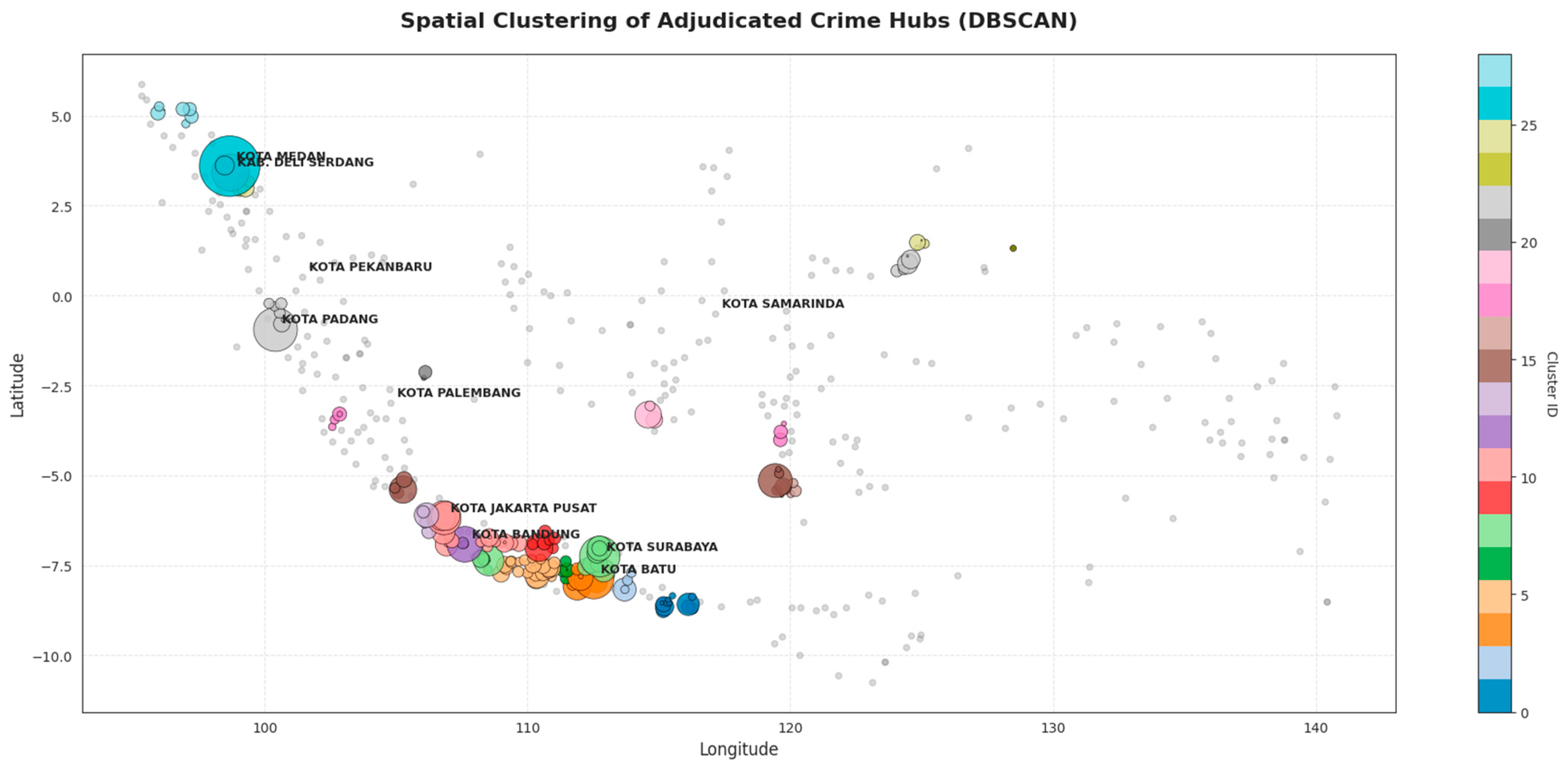
As illustrated in Figure 14, the spatial distribution of adjudicated crime reveals a high degree of regional concentration, particularly along the maritime and transit corridors of Java and Sumatra. The model identified 29 distinct adjudicated crime hubs, effectively isolating high-density metropolitan ecosystems from the background “noise” of geographically dispersed incidents.

The visualization confirms that while high-volume jurisdictions exist across the archipelago, they often function as “anchors” for larger regional corridors. The identification of these hubs is a critical finding, as it suggests that the “pressure” on the Indonesian court system is not evenly distributed but is focused within specific spatio-temporal nodes.

4.6.2. Analysis of Primary Adjudicated Crime Hubs

The clustering results provide an empirical basis for identifying the most pressurized zones in the country. The following hubs emerged as the primary “gravity centers”:

• The Mebidang Adjudicated Crime Hub (Cluster 26): Located in North Sumatra, this light-blue cluster (shown in the top left of Figure 14) successfully integrates Medan (4046 cases) with Deli Serdang (1532 cases) and Binjai (397 cases). This represents the highest combined volume of adjudicated crime in Western Indonesia, confirming that these jurisdictions share a continuous spatio-temporal pulse that transcends city borders.
• The East Java Multi-Hub System (Clusters 4, 8, and 3): East Java exhibits a complex multi-hub structure rather than a single provincial concentration. The Malang Raya Adjudicated Crime Hub (Cluster 4) successfully links Kota Batu (1716 cases) and Kota Malang (503 cases), proving that they function as a singular judicial unit. Meanwhile, the Surabaya Axis (Cluster 8) anchors the coastal region, and Cluster 3 indicates a high-volume corridor in the south (Tulungagung, Kediri, and Blitar).
• The Java–Banten Mega-Corridor (Clusters 11, 12, and 13): The map reveals a nearly continuous chain of adjudicated crime activity. The Jakarta Core Hub (Cluster 11) integrates Pusat, Utara, and Barat, while the Bandung Raya Axis (Cluster 12) anchors the West Java interior. This “Mega-Corridor” reflects the intense urbanization and connectivity of the national capital region.

4.6.3. Isolated Adjudicated Crime Anchors vs. Regional Hubs

A notable finding of the spatial analysis is the identification of Isolated Adjudicated Crime Anchors. As shown by the gray noise points in Figure 14, several of the top-15 high-volume cities do not form clusters with neighboring jurisdictions:

•

Kota Pekanbaru (1479 cases).

•

Kota Palembang (1379 cases).

•

Kota Samarinda (1277 cases).

•

Kota Jambi (1062 cases).

Unlike the Mebidang or Jakarta hubs, these anchors operate in geographical isolation. Their high caseloads are generated by internal city dynamics rather than regional spillover. For the Indonesian Supreme Court and National Police (Polri), this identifies two distinct strategic needs:

• Hub-Level Synchronization: In regions like Cluster 26 or 11, where jurisdictions are spatially linked, resources can be shared through regional task forces and synchronized court schedules.
• Anchor-Level Fortification: Isolated cities like Palembang require self-contained, high-capacity infrastructure, as they cannot rely on the “overflow” capacity of neighboring courts.

5. Discussion

The operationalization of the STL-XGBoost forecasting framework, integrated with the identified spatial hubs and judicial funnel metrics, offers a transformative pathway for data-driven judicial administration in Indonesia. This section discusses the practical applications of the framework for resource planning and the critical ethical considerations that must govern its deployment.

5.1. Practical Application Exploration

By shifting from static, administrative-based planning to a dynamic, predictive model, central judicial authorities can optimize resource allocation with higher precision. The identification of 29 distinct adjudicated crime hubs provides a high-resolution map for human resource management, allowing for the implementation of a “hub-and-spoke” staffing model. In high-pressure jurisdictions such as the Medan–Deli Serdang corridor (Cluster 26), the system can proactively recommend the temporary deployment of circuit judges or the prioritization of digital courtroom infrastructure, effectively mitigating potential case backlogs before they manifest in the procedural pipeline.

Beyond personnel management, the integration of the judicial funnel analysis establishes a strategic link between law enforcement activity and correctional capacity. While police-reported statistics (BPS) provide a general gauge of public safety, the adjudicated forecasts developed in this study provide a six-month lead time on the volume of final verdicts that will directly impact prison occupancy and prosecutorial workloads. For instance, the high adjudication rate identified in provinces like Riau (33.43%) signals an immediate requirement for prison capacity readiness following a predicted crime surge, whereas in jurisdictions like Jakarta (4.91%), the high attrition rate indicates that the immediate pressure on long-term correctional facilities remains proportionally lower despite high reporting volumes. This foresight allows the Attorney General’s office to reallocate specialized prosecutorial teams to specific regional hubs based on the predicted categorical crime typologies, such as anticipated surges in narcotics cases in urban centers.

From an engineering and deployment perspective, operationalizing this framework requires a robust data pipeline and scalable computational architecture. The current STL-XGBoost model, trained on the full 95,666-record dataset, requires approximately 20 min of processing on a standard cloud virtual machine (16-core CPU, 64 GB RAM), with GridSearchCV hyperparameter optimization representing the most computationally intensive stage. For a production system, a batch-processing architecture is recommended, with a daily data ingestion job triggered at 02:00 local time (UTC + 7 to UTC + 9) to pull new records from the Supreme Court’s case management API. Models should be retrained on a weekly or bi-weekly cadence to adapt to evolving temporal patterns without incurring excessive computational overhead. The pipeline should be containerized and orchestrated by a workflow manager to ensure reproducibility and portability across cloud environments. Predictive outputs, comprising daily forecasts per jurisdiction, should be stored in a time-series database and exposed through a REST API for use by judicial administrators through a front-end dashboard.

A key operational constraint for nationwide deployment is Indonesia’s inherently decentralized judicial infrastructure, where courts and prosecution offices across 38 provinces maintain locally siloed records, a challenge that the current centralized architecture does not yet address. Nevertheless, the quantified attrition gap documented in this research provides an empirical baseline for evaluating the systemic impact of emerging restorative justice (RJ) policies. By monitoring the delta between predicted judicial volume and actual adjudicated outcomes, policy-makers can quantitatively assess whether diversion programs successfully reduce court burden or whether a widening gap indicates a loss of procedural efficiency. This transforms the model from a simple predictive tool into a policy validation framework, enabling a feedback loop where digital justice interventions can be adjusted based on their measurable impact on the judicial funnel. Together, these applications demonstrate how spatio-temporal intelligence can move the judiciary toward a more resilient, evidence-based management paradigm.

5.2. Ethical Considerations and Algorithmic Fairness

While this framework offers a powerful tool for resource management, its implementation demands careful consideration of ethical and fairness implications. Adjudicated data, while more reliable than police reports, are not free from systemic biases. The patterns identified may reflect the spatial distribution of not only crime but also policing intensity, prosecutorial discretion, and socioeconomic factors that influence which cases reach a final verdict. There is a significant risk that the model could inadvertently create a self-perpetuating feedback loop: forecasting higher caseloads in a particular region may lead to the allocation of more judicial resources, which in turn could increase the adjudication rate in that area, thus confirming the model’s original prediction and potentially entrenching existing inequalities. To mitigate this, any deployment must be accompanied by regular algorithmic audits to test for disparate impacts on different demographic groups and geographical areas. Furthermore, the model’s outputs should be used strictly for internal resource allocation and should never be used as a direct input for proactive policing or pre-trial detention decisions, which could infringe on civil liberties. All data used in this study were fully de-identified, and city-level aggregation further ensures individual privacy.

6. Conclusions

This paper presents a multi-level spatio-temporal forecasting framework for adjudicated crime in Indonesia, integrating a hybrid STL-XGBoost model for temporal prediction with DBSCAN for spatial clustering. Drawing on 95,666 adjudicated crime records from the Supreme Court of Indonesia spanning January 2023 to June 2024, this research addresses a critical gap in the crime forecasting literature: the systematic underutilization of adjudicated judicial data as a reliable, verified signal for forecasting judicial workload and informing resource allocation decisions.

Temporal analysis confirmed the presence of a dominant seven-day weekly seasonality, and the optimized hybrid STL-XGBoost model achieved an R² of 0.8070 and sMAPE of 9.76% on the held-out test set. Multi-level spatial extension revealed a hierarchical predictive decay across administrative scales, while DBSCAN analysis identified 29 distinct adjudicated crime hubs concentrated in Java and Sumatra. Comparative analysis of reported versus adjudicated crime data revealed a systematic judicial funnel attrition ranging from 199.12% in Riau to 2436.02% in Papua, confirming that adjudicated data are a reliable predictor of judicial workload, not a comprehensive census of social deviance.

In conclusion, a hybrid STL-XGBoost and DBSCAN framework, applied to adjudicated judicial records, constitutes a technically rigorous and practically viable approach to multi-level crime forecasting in a large, geographically complex developing nation. The framework’s capacity to operate across national, provincial, and city scales, combined with its interpretable feature importance rankings and validated spatial clustering outputs, positions it as a decision support tool for judicial administrators, policy-makers, and law enforcement agencies seeking to transition from reactive to evidence-based, data-driven governance in Indonesia’s justice sector.

6.1. Limitations

Several limitations of the present study warrant acknowledgement. The 18-month observation window, while sufficient for identifying weekly and monthly cycles, may not capture longer-term structural shifts in judicial processing patterns or the effects of major policy-level interventions. The use of city centroids as spatial proxies for DBSCAN, necessitated by the absence of precise incident-level geographic coordinates in the national judicial record, introduces a degree of ecological fallacy that future research should address through the incorporation of finer-grained geocoded data. The chronological single-split validation approach, while appropriate for simulating real-world forecasting scenarios, does not account for potential non-stationarity arising from changes in judicial processing practices over time; rolling-origin or blocked cross-validation schemes represent a methodologically richer alternative for future work. Furthermore, the dataset encompasses 11 crime categories that may exhibit heterogeneous temporal dynamics, and category-specific forecasting models could yield additional predictive granularity beyond the aggregate framework presented here.

6.2. Future Research Directions

Future research directions include the extension of the framework to incorporate real-time data streams from court management systems, enabling near-real-time judicial workload monitoring. The integration of socioeconomic shock variables such as unemployment rates, commodity price fluctuations, and natural disaster indicators could further improve the model’s capacity to anticipate stochastic crime spikes that fall outside the deterministic seasonal patterns captured through STL decomposition. Addressing the decentralization constraint identified in Section 5.1, a particularly critical future direction concerns the transition to a distributed learning framework. Indonesia’s judicial infrastructure is inherently decentralized: courts, police stations, and prosecution offices across 38 provinces maintain locally siloed records, and many remote jurisdictions in Papua, Maluku, and Nusa Tenggara operate under severe bandwidth constraints. Recent advances in distributed first-order optimization with log-scale quantization [47] offer a technically viable pathway for aggregating model updates across provincial nodes without requiring the centralization of sensitive raw judicial data, a critical consideration for institutional adoption. Such architecture would also enable continuous model retraining as new case records are generated, overcoming the temporal staleness inherent in the current 18-month snapshot. Additionally, the development of category-specific spatio-temporal models for high-prevalence offense types such as narcotics and property crime could provide more actionable intelligence for specialized judicial units, moving beyond the aggregate forecasting framework presented here.

References

1. BPS-Statistics Indonesia. Crime Statistics 2022; BPS-Statistics Indonesia: Jakarta, Indonesia, 2022; Volume 13. Available online: https://www.bps.go.id/id/publication/2022/11/30/4022d3351bf3a05aa6198065/statistik-kriminal-2022.html (accessed on 16 December 2025).
2. BPS-Statistics Indonesia. Crime Statistics 2023; BPS-Statistics Indonesia: Jakarta, Indonesia, 2023; Volume 14. Available online: https://www.bps.go.id/id/publication/2023/12/12/5edba2b0fe5429a0f232c736/statistik-kriminal-2023.html (accessed on 17 December 2025).
3. BPS-Statistics Indonesia. Crime Statistics 2024; BPS-Statistics Indonesia: Jakarta, Indonesia, 2024; Volume 15. Available online: https://www.bps.go.id/id/publication/2024/12/12/13317138a55b2f7096589536/statistik-kriminal-2024.html (accessed on 12 January 2026).
4. BPS-Statistics Indonesia. Crime Statistics 2024/2025; BPS-Statistics Indonesia: Jakarta, Indonesia, 2025; Volume 16. Available online: https://www.bps.go.id/id/publication/2025/12/12/2edc8ea4c35b19ba912fc7e4/statistik-kriminal-2024-2025.html (accessed on 13 January 2026).
5. Brantingham, P.; Brantingham, P. Criminality of Place Crime Generators and Crime Attractors. Eur. J. Crim. Policy Res. 1995, 3, 5–26. [Google Scholar] [CrossRef] [Scilit]
6. Jonathan, O.E.; Olusola, A.J.; Bernadin, T.C.A.; Inoussa, T.M. Impacts of Crime on Socio-Economic Development. Mediterr. J. Soc. Sci. 2021, 12, 71. [Google Scholar] [CrossRef] [Scilit]
7. Berk, R.; Bleich, J. Statistical procedures for forecasting criminal behavior: A comparative assessment. Criminol. Public Policy 2013, 12, 513–544. [Google Scholar] [CrossRef] [Scilit]
8. Al Boni, M.; Gerber, M.S. Area-Specific Crime Prediction Models. In Proceedings of the 15th IEEE International Conference on Machine Learning and Applications (ICMLA), Anaheim, CA, USA, 18–20 December 2016. [Google Scholar] [CrossRef] [Scilit]
9. Ramos-Maqueda, M.; Chen, D.L. The data revolution in justice. World Dev. 2025, 186, 106834. [Google Scholar] [CrossRef] [Scilit]
10. Yunus, A.; Loo, J. London street crime analysis and prediction using crowdsourced dataset. J. Comput. Math. Data Sci. 2024, 10, 100089. [Google Scholar] [CrossRef] [Scilit]
11. Chen, T.; Guestrin, C. XGBoost: A Scalable Tree Boosting System. In Proceedings of the 22nd ACM SIGKDD International Conference on Knowledge Discovery and Data Mining, San Francisco, CA, USA, 13–17 August 2016; pp. 785–794. [Google Scholar]
12. Ester, M.; Kriegel, H.-P.; Sander, J.; Xu, X. A density-based algorithm for discovering clusters. In Proceedings of the Second International Conference on Knowledge Discovery and Data Mining, Portland, OR, USA, 2–4 August 1996; pp. 226–231. [Google Scholar]
13. Mohammed, A.; Baiee, W. The GIS based Criminal Hotspot Analysis using DBSCAN Technique. In IOP Conference Series: Materials Science and Engineering; IOP Publishing: Bristol, UK, 2020; Volume 928, p. 032081. [Google Scholar] [CrossRef] [Scilit]
14. Mungekar, D.; Joshi, H.; Kankekar, A.; Nair, P.; Das, P. Crime Analysis using DBSCAN Algorithm. In Proceedings of the 2021 Third International Conference on Inventive Research in Computing Applications (ICIRCA), Coimbatore, India, 2–4 September 2021; pp. 628–635. [Google Scholar] [CrossRef] [Scilit]
15. Weisburd, D.; Lum, C. The diffusion of computerized crime mapping in policing: Linking research to practice. Police Pract. Res. 2005, 6, 419–434. [Google Scholar] [CrossRef] [Scilit]
16. Cohen, L.E.; Felson, M. Social change and crime rate trends: A routine activity approach. Am. Sociol. Rev. 1979, 44, 588–608. [Google Scholar] [CrossRef] [Scilit]
17. Brantingham, P.J.; Brantingham, P.L. Environmental Criminology; Waveland Press: Long Grove, IL, USA, 1991. [Google Scholar]
18. Khare, I.S.; Martheswaran, T.K.; Thomas, R.K.; Bora, A. Actionable Insights on Philadelphia Crime Hot-Spots: Clustering and Statistical Analysis to Inform Future Crime Legislation. arXiv 2023, arXiv:2306.15987. [Google Scholar] [CrossRef] [Scilit]
19. Cesario, E.; Uchubilo, P.I.; Vinci, A.; Zhu, X. Discovering multi-density urban hotspots in a smart city. In Proceedings of the 2020 IEEE International Conference on Smart Computing (SMARTCOMP); IEEE: Piscataway, NJ, USA, 2020; pp. 332–338. [Google Scholar] [CrossRef] [Scilit]
20. Perry, W.L.; McInnis, B.; Price, C.C.; Smith, S.C.; Hollywood, J.S. Predictive Policing: The Role of Crime Forecasting in Law Enforcement Operations; RAND Corporation: Santa Monica, CA, USA, 2013. [Google Scholar]
21. Brantingham, P.; Brantingham, P. Crime Pattern Theory. In Environmental Criminology and Crime Analysis; Wortley, R., Mazerolle, L., Eds.; Willan Publishing: Cullompton, UK, 2008; pp. 78–93. [Google Scholar]
22. Ratcliffe, J.H. Intelligence-Led Policing, 2nd ed.; Routledge: London, UK, 2016. [Google Scholar]
23. Dakalbab, F.; Talib, M.A.; Waraga, O.A.; Nassif, A.B.; Abbas, S.; Nasir, Q. Artificial intelligence & crime prediction: A systematic literature review. Soc. Sci. Humanit. Open 2022, 6, 100342. [Google Scholar] [CrossRef] [Scilit]
24. Abubaker, H.; Muchtar, F.; Degan, K.S.; Azmi, K.H.M.; Hamid, F.K.A.; Along, N.Z.B.; Khairuddin, A.R.B. Crime prediction based on classification approaches. Procedia Comput. Sci. 2025, 259, 1407–1415. [Google Scholar] [CrossRef] [Scilit]
25. Yu, C.-H.; Ward, M.W.; Morabito, M.; Ding, W. Crime forecasting using data mining techniques. In Proceedings of the 2011 IEEE 11th International Conference on Data Mining Workshops, Vancouver, BC, Canada, 11 December 2011; pp. 779–786. [Google Scholar]
26. Ratcliffe, J.H. Crime mapping: Spatial and temporal challenges. In Handbook of Quantitative Criminology; Piquero, A.R., Weisburd, D., Eds.; Springer: New York, NY, USA, 2010; pp. 5–24. [Google Scholar]
27. Deswandi, A.; Hastomo, W. Predicting Crime Time Intervals Using Machine Learning Models. J. Inf. Syst. Inform. 2024, 6, 2397–2418. [Google Scholar] [CrossRef] [Scilit]
28. Krichen, M.; Mihoub, A. Long Short-Term Memory Networks: A Comprehensive Survey. AI 2025, 6, 215. [Google Scholar] [CrossRef] [Scilit]
29. Bento, J.; Saleiro, P.; Cruz, A.F.; Figueiredo, M.A.T.; Bizarro, P. TimeSHAP: Explaining Recurrent Models through Sequence Perturbations. In Proceedings of the 27th ACM SIGKDD Conference on Knowledge Discovery & Data Mining, Singapore, 14–18 August 2021; pp. 2565–2573. [Google Scholar] [CrossRef] [Scilit]
30. Hyndman, R.J.; Athanasopoulos, G. Forecasting: Principles and Practice, 3rd ed.; OTexts: Melbourne, Australia, 2021; Available online: https://otexts.com/fpp3/ (accessed on 11 March 2026).
31. Taylor, S.J.; Letham, B. Forecasting at Scale. Am. Stat. 2018, 72, 37–45. [Google Scholar] [CrossRef] [Scilit]
32. Yadav, S. A Comparative Study of ARIMA, Prophet and LSTM for Time Series Prediction. J. Artif. Intell. Mach. Learn. Data Sci. 2024, 1, 1813–1816. [Google Scholar] [CrossRef] [Scilit]
33. Cichosz, P. Urban Crime Risk Prediction Using Point of Interest Data. ISPRS Int. J. Geo-Inf. 2020, 9, 459. [Google Scholar] [CrossRef] [Scilit]
34. Butt, U.M.; Letchmunan, S.; Hassan, F.H.; Ali, M.; Baqir, A.; Sherazi, H.H.R. Spatio-Temporal Crime HotSpot Detection and Prediction: A Systematic Literature Review. IEEE Access 2020, 8, 166553–166574. [Google Scholar] [CrossRef] [Scilit]
35. Chainey, S.; Ratcliffe, J. GIS and Crime Mapping; John Wiley & Sons: Hoboken, NJ, USA, 2013. [Google Scholar]
36. Sui, J.; Chen, P.; Gu, H. Deep Spatio-Temporal Graph Attention Network for Street-Level 110 Call Incident Prediction. Appl. Sci. 2024, 14, 9334. [Google Scholar] [CrossRef] [Scilit]
37. Ramadan, A.; Rantini, D.; Triangga, Y.; Ningrum, R.A.; Othman, F. Space-Time Autoregressive Integrated Moving Average (STARIMA) Modeling for Predicting Criminal Cases of Motor Vehicle Theft in Surabaya, Indonesia. Data Metadata 2024, 3, 621. [Google Scholar] [CrossRef] [Scilit]
38. Fan, Y.; Hu, X.; Hu, J. Research on a Crime Spatiotemporal Prediction Method Integrating Informer and ST-GCN: A Case Study of Four Crime Types in Chicago. Big Data Cogn. Comput. 2025, 9, 179. [Google Scholar] [CrossRef] [Scilit]
39. Huang, Y.; Yang, B.; Ren, X.; Lu, Y.; Lan, M.; Gong, X. Spatio-temporal cokriging crime predictions using social media data: A multi-type case study in San Jose, California. Comput. Urban Sci. 2025, 5, 72. [Google Scholar] [CrossRef] [Scilit]
40. Olatunbosun, O.A.; Oluduro, O. Crime Forecasting and Planning in Developing Countries: Emerging Issues. Can. Soc. Sci. 2012, 8, 36–43. [Google Scholar] [CrossRef]
41. Meijer, A.; Wessels, M. Predictive Policing: Review of Benefits and Drawbacks. Int. J. Public Admin. 2019, 42, 1031–1039. [Google Scholar] [CrossRef] [Scilit]
42. Galiani, S.; Jaitman, L. Predictive Policing in a Developing Country: Evidence from Two Randomized Controlled Trials. J. Quant. Criminol. 2022, 39, 805–831. [Google Scholar] [CrossRef] [Scilit]
43. Chapman, P.; Clinton, J.; Kerber, R.; Khabaza, T.; Reinartz, T.; Shearer, C.; Wirth, R. CRISP-DM 1.0: Step-by-Step Data Mining Guide; SPSS Inc.: Chicago, IL, USA, 2000. [Google Scholar]
44. Schröer, C.; Kruse, F.; Gómez, J.M. A Systematic Literature Review on Applying CRISP-DM Process Model. Procedia Comput. Sci. 2021, 181, 526–534. [Google Scholar] [CrossRef] [Scilit]
45. Martínez-Plumed, A.; Contreras-Ochando, L.; Ferri, C.; Hernández-Orallo, J.; Kull, M.; Lachiche, N.; Ramírez-Quintana, M.J.; Flach, P. CRISP-DM Twenty Years Later: From Data Mining Processes to Data Science Trajectories. IEEE Trans. Knowl. Data Eng. 2019, 33, 3048–3061. [Google Scholar] [CrossRef] [Scilit]
46. United Nations Office on Drugs and Crime. International Classification of Crime for Statistical Purposes (ICCS), Version 1.0; UNODC: Vienna, Austria, 2015. [Google Scholar]
47. Doostmohammadian, M.; Qureshi, M.I.; Khalesi, M.H.; Rabiee, H.R.; Khan, U.A. Log-Scale Quantization in Distributed First-Order Methods: Gradient-Based Learning From Distributed Data. IEEE Trans. Autom. Sci. Eng. 2025, 22, 10948–10959. [Google Scholar] [CrossRef] [Scilit]
Figure 1. Analysis of annual reported crime trends in Indonesia (2020–2023) based on BPS data. Blue bars represent annual volume, while the purple line depicts the growth trajectory. The large purple upward arrow signifies the post-pandemic surge, and the small blue downward arrow indicates the transient decline during the pandemic.
Information 17 00331 g001
Figure 2. Theoretical framework [15,16,17].
Information 17 00331 g002
Figure 3. Research methodology based on CRISP-DM framework. Dark blue squares identify the six primary phases; lavender and teal boxes indicate objectives and sub-tasks, respectively. White bulleted boxes detail the phase-specific implementation.
Information 17 00331 g003
Figure 4. Periodogram of daily crime counts. The power spectrum identifies dominant frequencies, with a prominent peak at T = 7 days representing the weekly seasonal cycle. The red horizontal line at the zero-power baseline serves as a reference axis to provide a clear visual anchor for the spectral density spikes, highlighting their magnitude relative to the origin.
Information 17 00331 g004
Figure 5. Chronological data splitting for crime forecasting.
Information 17 00331 g005
Figure 6. k-distance plot for epsilon ϵ selection. The blue solid line represents the sorted distances of each city centroid to its k-th nearest neighbor (k=3). The curve visualizes a distinct "elbow" at approximately 0.1°.
Information 17 00331 g006
Figure 7. Temporal analysis of daily adjudicated crime incidents (January 2023: June 2024). (a) Time series where the grey line represents the raw observed daily counts and the red line denotes the 30-day moving average used to identify baseline stability. (b) Probability distribution where the shaded bars indicate the frequency of daily incident counts (histogram) and the blue curve represents the Kernel Density Estimate (KDE), illustrating the statistical distribution and slight right-skew of the data.
Information 17 00331 g007
Figure 8. Spectral and correlation diagnostics of the adjudicated crime series. (a) Periodogram identifying the dominant seven-day frequency, where the teal curve represents spectral power and the vertical red dashed line marks the peak at T = 7 days. (b) Autocorrelation Function (ACF) and (c) Partial Autocorrelation Function (PACF) of residuals. In panel (b), blue stems represent coefficients, while in panel (c), green stems are used; the shaded regions in both panels indicate the 95% confidence intervals. Spikes exceeding these boundaries (notably at Lag 1 and Lag 28 in the PACF) denote the statistically significant dependencies utilized for model feature engineering.
Information 17 00331 g008
Figure 9. Relative distribution of adjudicated crime types (top 15 cities).
Information 17 00331 g009
Figure 10. (a) Comparative visualization of the Indonesian Judicial Funnel (2023). Comparison of reported volume (BPS) versus adjudicated outcomes on a logarithmic scale, highlighting the magnitude of caseload attrition; (b) Provincial adjudication rates (%), where higher percentages (such as Riau at 33.43%) indicate a more direct transition from initial report to final judicial verdict.
Information 17 00331 g010
Figure 11. STL decomposition of the national adjudicated crime series. (a) Observed daily incident counts; (b) isolated trend component T t showing localized shifts; (c) seasonal component S t reflecting the consistent seven-day cycle; (d) stochastic residuals R t representing the stationary signal used for XGBoost training.
Information 17 00331 g011
Figure 12. Comparison of actual vs. predicted daily crime incidents. The upper panel displays the alignment between the observed counts and the reconstructed STL-XGBoost forecast for the test set (April–June 2024); the lower panel illustrates the residual error, highlighting the model’s consistency across both high- and low-volume periods.
Information 17 00331 g012
Figure 13. XGBoost feature importance (Gini Importance).
Information 17 00331 g013
Figure 14. Spatial clustering of adjudicated crime hubs (DBSCAN). Bubble sizes represent the normalized adjudicated crime volume per city centroid, while distinct colors identify unique regional clusters optimized at epsilon = 0.3 and minPts = 3. Gray markers denote ‘noise’ points, representing isolated jurisdictions. The overlapping bubbles in high-density regions (e.g., the Java-Sumatra corridor) are a deliberate visualization of the geographical proximity and high-volume connectivity between neighboring courts, effectively mapping the "adjudicated crime hubs" as functional, interconnected legal ecosystems rather than isolated incidents.
Information 17 00331 g014