


Abstract
This paper presents a comprehensive comparative study of deep learning approaches for clustering mathematical functions based on their behavioral patterns. We investigate three distinct embedding strategies: autoencoder-based unsupervised learning, supervised classification with learned embeddings, and direct convolutional feature extraction. Each approach transforms continuous functions into meaningful vector representations that capture essential mathematical characteristics. Through extensive experimentation and multiple visualization techniques, we demonstrate that supervised learning with explicit function type guidance produces the most discriminative embeddings, achieving average silhouette score 0.6. Our findings provide valuable insights into the relative effectiveness of different representation learning paradigms for mathematical function analysis.
1. Introduction
Mathematical functions are the language of science and engineering, describing relationships between variables in everything from physical laws to economic models. Traditional approaches to analyzing collections of functions often rely on symbolic comparison [1], which can be inefficient for large datasets and overly sensitive to differences in syntactic form. For instance, symbolic solvers may struggle to readily equate mathematically identical functions presented in varying analytical forms, such as versus (x + 1), where , especially when dealing with highly perturbed, unsimplified, or non-standard representations. Other methods include visual inspection [2], which quickly becomes impractical as the number of functions grows, and manual feature extraction, which is time-consuming and demands significant expert knowledge.
To address these limitations, modern methods treat functions as data objects that can be embedded into a space where similarity can be measured quantitatively. Functional Data Analysis (FDA) [3,4] provides the classical statistical foundation for this, offering tools for regression and classification while ensuring interpretability. This approach is based on the assumption that observed measurements are merely snapshots of a smooth, continuous process. Therefore, the focus is on inferring function properties such as rate of change and acceleration, rather than solely on individual values. To achieve this, discrete data is transformed into a functional representation using base functions, such as Fourier series for periodic data or B-splines for non-periodic data. This allows for information compression, noise reduction, and improved analyzability. However, FDA often relies on basis expansions or smoothing [5], which may fail for highly irregular functions.
Unlike manually engineered features, representation learning [6] provides a more flexible alternative by automatically discovering useful features from data, much like word2vec [7] in Natural Language Processing (NLP) or convolutional neural networks (CNNs) in computer vision. This is realized by transforming raw data—such as text or images—into mathematical vectors within multidimensional spaces, so that semantically similar data becomes geometrically similar within this space, facilitating processing and analysis. This enables scalable and expressive embeddings but requires large datasets and careful regularization to avoid overfitting.
Neural operators [8] take this idea a step further by learning mappings between entire function spaces, capturing rich functional relationships and generalizing across resolutions, though at the cost of model complexity and interpretability. Instead of learning a function that relates specific inputs to specific outputs, as in traditional models, these approaches learn a complete mathematical operator that relates infinitely large function spaces. These models exhibit discretization invariance, meaning they can be trained on low-precision data and then used to make predictions at much higher precision without retraining. This feature provides a highly practical ability to rapidly simulate complex physical phenomena while maintaining robust performance across different precision levels.
Our approach builds on these ideas, combining the interpretability of FDA with the flexibility of representation learning, using neural embeddings to enable efficient, scalable comparison and function clustering.
We hypothesize that functions can be represented in a semantic embedding space where the geometric distance between function embeddings corresponds to the similarity of their behavior. This allows us to leverage the powerful unsupervised machine learning tools of data clustering [9] to automatically organize and discover patterns within a large corpora of functions.
We considered that different representation learning paradigms will yield embeddings with varying clustering properties and that explicit supervision can guide the learning process toward more discriminative representations. Our work makes two key contributions:
- •
- It presents a systematic comparison of three embedding strategies for function representation, where we evaluate the impact of different approaches on the quality of function representations.
- •
- It performs a comprehensive evaluation using visualization and multiple clustering quality metrics to verify and evaluate the performance.
2. Materials and Methods
2.1. Function Generation and Representation
We generated a diverse dataset of 600 functions: across five semantic types, sampled over the interval with 128 points to balance resolution and computational efficiency. The function parameters (denoted as a, b, and c in the defining equations) were independently drawn from a uniform continuous distribution . To simulate realistic observational conditions and sensor inaccuracies, additive Gaussian noise (0, was introduced to the final signal.
The dataset is strictly balanced, with each of the five function types constituting exactly 20% of the total dataset (120 samples per class), eliminating the need for class imbalance corrections:
- •
- Linear: ;
- •
- Quadratic: ;
- •
- Exponential: ;
- •
- Trigonometric: ;
- •
- Logarithmic: (for the logarithmic class, we enforce a positive log argument using |b| + 1).
2.2. Embedding Strategies
Before using any model, each generated mathematical function (linear, quadratic, etc.) is
- •
- Represented as a 1D array of 128 sample points (the y-values of the function from x = [−3, 3]).
- •
- Normalized to have mean ≈ 0 and standard deviation ≈ 1 using z-score normalization. This step ensures scale invariance, preventing functions with naturally larger amplitudes (e.g., exponential) from dominating the loss function during training, while preserving the relative shape and behavioral characteristics essential for clustering.
- •
- Reshaped into a 3D tensor (samples, 128, 1) for CNN input.
Then, three different deep learning architectures were employed to learn low-dimensional embeddings for the functions, enabling the extraction of meaningful latent representations that capture structural and semantic similarities across the dataset.
2.2.1. Autoencoder-Based Embeddings (Unsupervised)
The autoencoder approach [4,10] learns compressed representations through reconstruction, enabling the model to capture the most salient features of the input data while minimizing reconstruction error.
By forcing the network to reconstruct the original functions X from their compressed representations Z, the autoencoder encourages the bottleneck layer to capture the most salient features necessary for accurate reconstruction. Formally, the encoder maps the input data to a low-dimensional latent space, and the decoder reconstructs the input from this latent code.
Minimizing the reconstruction loss (Equation (1)) ensures that encodes the essential structure of X, while discarding irrelevant or redundant information.
The architecture employed consists of an encoder, bottleneck, and decoder set up as follows:
- •
- Encoder: Three 1D convolutional layers (32, 64, 128 filters) with kernel sizes of 15, 10, and 5, respectively.
- •
- Bottleneck: A 32-dimensional embedding layer.
- •
- Decoder: A symmetric transposed convolutional architecture.
The network was trained using the mean squared error (MSE) reconstruction loss function and optimized with the Adam optimizer at a learning rate of 0.001. To prevent overfitting and improve generalization, regularization techniques such as batch normalization, dropout (ranging from 0.1 to 0.2), and L2 weight regularization (1 × 10⁻⁴) were applied.
2.2.2. Supervised Classification Embeddings
This approach leverages explicit function-type labels to guide the learning of representations. Instead of learning latent features solely through reconstruction, the network is trained to predict the function class, encouraging the embeddings to capture features that are discriminative across labeled categories. Formally, given input functions X with corresponding labels y, the encoder maps the input to a latent space Z, which is then passed to a classification head . The network is optimized using a cross-entropy loss , where represents the ground-truth function class labels and denotes the predicted class probabilities produced by the classifier head. This ensures that the latent representation Z contains information relevant for distinguishing between function types.
The network uses a feature extractor, embedding layer, and classifier head set up as follows:
- •
- Feature Extractor: Three 1D convolutional layers (32, 64, 128 filters) identical to autoencoder.
- •
- Embedding Layer: A 32-dimensional linear projection.
- •
- Classifier Head: Two fully connected layers (64, 5 units) with activation.
The model is trained using categorical cross-entropy loss with the Adam optimizer at a learning rate of 0.001, ensuring that the embeddings encode discriminative information relevant for accurate function classification.
The embedding layer is optimized to produce representations that are linearly separable with respect to function-type labels y. By minimizing the categorical cross-entropy loss between predicted probabilities and true labels , the network encourages the latent space to encode discriminative features, ensuring that functions from different classes are well separated while maintaining compact and informative embeddings.
2.2.3. Simple CNN Embeddings
This approach employs a lightweight convolutional neural network [11] designed to produce embeddings without any explicit training objective. It aims to evaluate the contribution of learned versus random feature representations. The network uses a series of lightweight 1D convolutional layers [12] to extract hierarchical features from the input signal with the following architecture:
- •
- Three 1D convolutional layers, each followed by batch normalization and pooling.
- •
- A global average pooling layer to aggregate spatial information.
- •
- A final 32-dimensional linear projection to obtain compact embeddings.
The model is not explicitly trained on any supervised or unsupervised objective. Instead, its parameters remain randomly initialized, and the network operates in a frozen state throughout. This design intentionally removes the influence of learning, allowing the extracted embeddings to serve as a baseline for comparison against models with trained representations. By contrasting performance with and without learning, this setup helps quantify the intrinsic structure captured by random convolutional filters and highlights the added value of representation learning. To ensure the reliability of this baseline, the Simple CNN was evaluated using 30 different random seeds, with the reported metrics representing the mean ± standard deviation to account for initialization variance.
This approach acts as a control or baseline, allowing comparison with other trained models. By observing how randomly initialized features perform in downstream tasks, one can quantify the value of learned representations, isolating what is gained through supervised or self-supervised learning.
2.3. Clustering
The embeddings are normalized and then clustered using the K-Means algorithm [13]. The number of clusters K is set to the number of known function types in the generated data (5) to evaluate the method’s accuracy. The cluster assignments are given by (Equation (2)):
where
- •
- is the centroid of the ith cluster.
- •
- represents the feature vector (embedding) of data point f.
Specifically, data point is assigned to the cluster whose centroid is closest (in squared Euclidean distance) to its feature vector .
3. Experiments
To evaluate the efficacy of the proposed representation learning techniques, we generated a synthetic dataset comprising 600 functions equally distributed across five distinct mathematical classes: linear, quadratic, exponential, trigonometric (sine and cosine), and logarithmic. These categories were selected to represent a diverse spectrum of monotonic and periodic behaviors, ensuring a challenging benchmark for feature extraction. Each function was sampled at 128 discrete points over the interval , standardized via z-score normalization to ensure scale invariance, and augmented with additive Gaussian noise to simulate the stochastic variability inherent in real-world signal data.
We implemented three distinct 32-dimensional embedding strategies based on 1D convolutional neural network (CNN) architectures, utilizing a series of convolutional blocks, max-pooling, and batch normalization to capture local patterns along the sampled input axis (x). These strategies included (1) an unsupervised autoencoder trained to minimize mean squared error (MSE) reconstruction loss, forcing the latent space to retain the most salient structural features of the input; (2) a supervised classifier optimized via cross-entropy loss to predict function labels, which encourages the formation of class-discriminative clusters; and (3) a randomly initialized CNN baseline to assess the inherent architectural bias and feature-extracting capacity of the network structure prior to any task-specific optimization.
Both trained models utilized the Adam optimizer, supplemented by early stopping criteria and learning rate reduction on plateau to mitigate overfitting and ensure stable convergence during the 50-epoch training cycle. Following feature extraction, the resulting high-dimensional embeddings were standardized and partitioned into five clusters using K-Means with n_{init} = 20 to guarantee robust centroid initialization. Clustering performance was quantitatively validated using three complementary intrinsic metrics: the silhouette score to assess cluster separation and individual point alignment, the Calinski–Harabasz Index to measure the ratio of between-cluster dispersion to within-cluster dispersion, and the Davies–Bouldin Index to evaluate the overall compactness and degree of overlap between the generated partitions.
4. Results and Analysis
4.1. Quantitative Performance Comparison
In order to compare model performance, clustering evaluation metrics and training stability were used, where the silhouette score [14] assesses intra-cluster cohesion and inter-cluster separation, the Calinski–Harabasz Index [15] measures cluster compactness relative to separation, the Davies–Bouldin Index [16] evaluates cluster overlap, and training stability quantifies the consistency of the clustering results across multiple training runs, reflecting the robustness of the models.
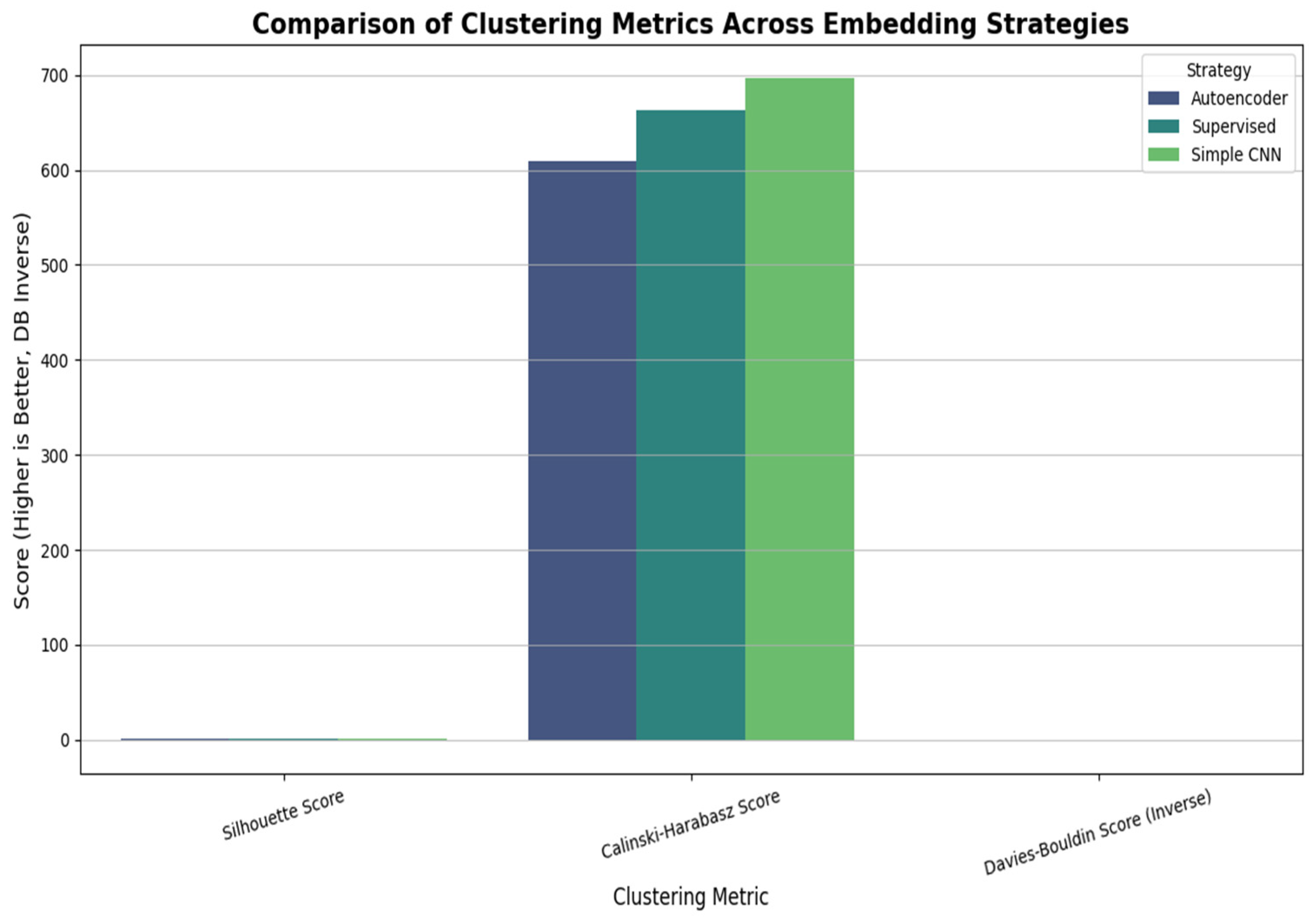
As seen in Table 1 and Figure 1, the supervised approach outperformed both unsupervised methods, demonstrating the value of explicit guidance in learning discriminative representations. This table reports the mean ± standard deviation across n = 30 independent runs (random seeds) for each method.
Table 1.
Embedding strategy performance metrics.
Figure 1.
Clustering metrics across embedding strategies. The x-axis denotes the embedding method and the y-axis denotes the metric value (higher silhouette and Calinski–Harabasz values indicate better separation/compactness, while lower Davies–Bouldin values indicate less overlap).
4.2. Embedding Space Analysis
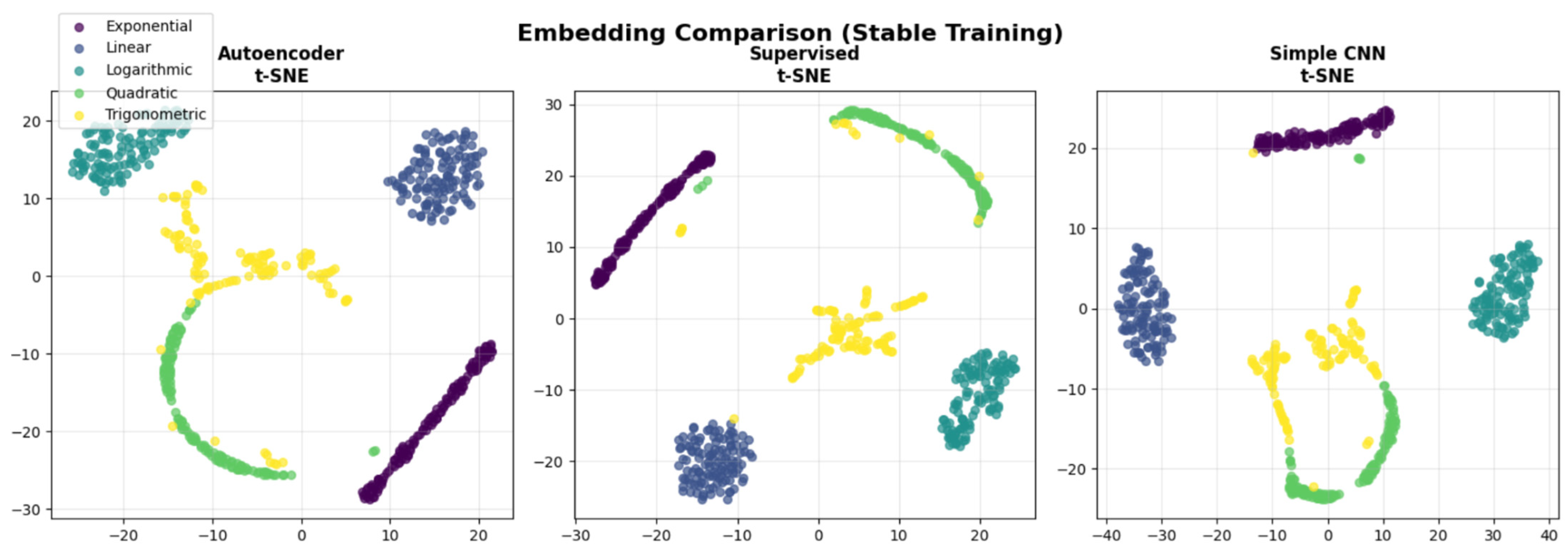
To analyze the quality and structure of the representations learned, we examine the embedding spaces produced by different models. Figure 2 presents a visual comparison of the resulting embeddings obtained using t-SNE [17] for dimensionality reduction, highlighting how each approach organizes the data in a lower-dimensional space and the extent to which meaningful structure emerges. This analysis provides insight into the models’ ability to capture latent patterns and achieve separability among underlying data groups.
Figure 2.
t-SNE visualization of learned embeddings (axes are dimensionless; proximity indicates similarity and absolute coordinate values are not interpretable). Different colors and markers correspond to the five distinct ground-truth mathematical function classes (linear, quadratic, exponential, trigonometric, and logarithmic).
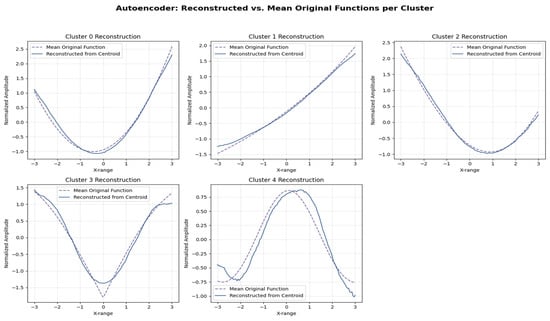
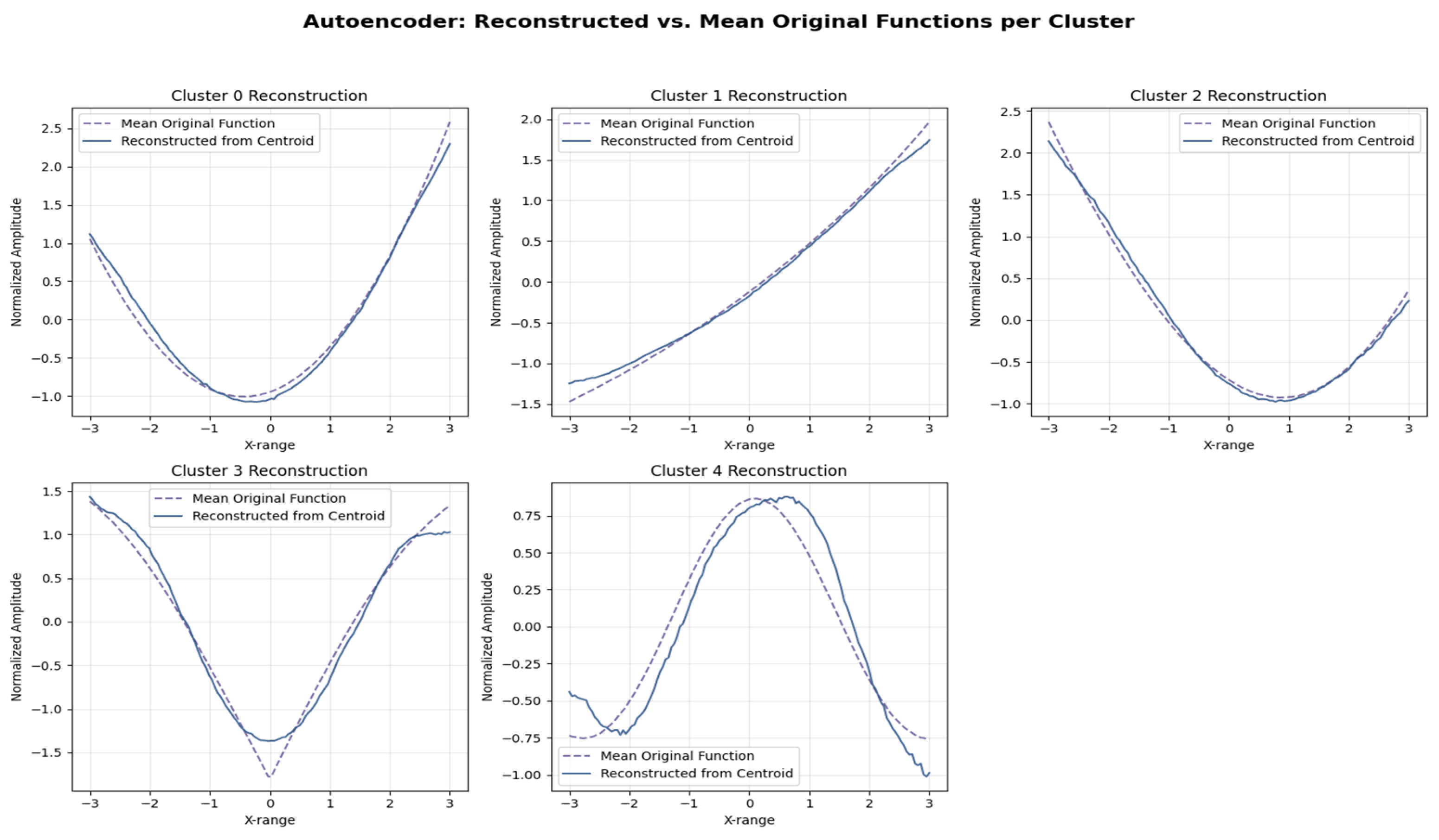
The analysis of the embedding spaces reveals clear differences in the quality of learned representations across models. The supervised embeddings clearly show the best separation of the five function types in the 2D projected space. The autoencoder produces partially separable clusters, indicating that it captures some intrinsic structure in the data, while the untrained CNN embeddings exhibit more overlap and less clear boundaries between the different function categories, particularly among classes with similar patterns. Figure 3 compares reconstructed functions from cluster centroids against the mean original functions within those clusters, indicating how well the autoencoder’s embeddings represent and capture function shapes.
Figure 3.
Autoencoder-reconstructed functions.
In contrast, the supervised model yields well-separated and highly compact clusters with minimal overlap, demonstrating strong class-discriminative representation learning and effective guided feature extraction. The simple CNN produces embeddings with moderate structure, where some classes are distinguishable, but cluster compactness and consistency are reduced, reflecting representations driven primarily by convolutional inductive biases rather than learned semantic abstractions. While these visualizations provide useful qualitative insights, they should be interpreted with caution, as two-dimensional projections (e.g., via t-SNE) can distort distances and neighborhood relationships in the original high-dimensional space and are sensitive to hyperparameter choices. Consequently, the visual analysis is complemented with quantitative clustering metrics and training stability measures to more reliably assess representation quality.
To better understand the structure of the learned embeddings, Table 2 presents a comparative analysis of clustering characteristics across models, including separation, compactness, overlap, and qualitative interpretation.
Table 2.
Comparison of the models’ embeddings clusters.
5. Discussion
It is worth mentioning here that the absolute increase in the silhouette score from 0.5 (in unsupervised learning) to 0.6 (supervised) may seem unremarkable, but in high-dimensional embedding spaces, even small improvements can reflect meaningfully better separation between closely related function families, where structural boundaries are often subtle. For this reason, we report clustering performance using complementary intrinsic metrics (silhouette, Calinski–Harabasz, and Davies–Bouldin) and summarize results as aggregated statistics across multiple runs, rather than making claims of statistical significance.
The results demonstrate the value of explicit supervision for learning function embeddings when labels are available, as function type labels guide the network toward discriminative features rather than reconstruction-oriented patterns, a behavior consistent with how functions are categorized based on global properties rather than local variations. Although autoencoder-based representations are less effective for clustering, they remain advantageous in unlabeled settings by capturing mathematically meaningful features that may support downstream tasks such as function approximation or symbolic regression.
Moreover, the strong performance of relatively simple convolutional architectures indicates that local pattern detection could be sufficient for function classification, with hierarchical feature learning enabling the capture of mathematical properties at multiple scales from local curvature and slope in shallow layers, through periodicity and growth trends in intermediate layers, to global function behavior in deeper layers.
From a practical perspective, these findings suggest using supervised models when function labels are available, autoencoder-based approaches in unsupervised scenarios, and hybrid or ensemble strategies to achieve robust performance across varying data conditions.
6. Conclusions
This comparative study demonstrates that deep learning-based embeddings can effectively capture the semantic properties of mathematical functions for clustering tasks, with the supervised learning approach achieving superior performance, as indicated by a silhouette score of 0.6, outperforming unsupervised methods. This improvement is driven by appropriate architectural design, the incorporation of training stability measures, and explicit supervision through function-type labels. It is important to note that this superior performance is validated here within the specific constraints of our generated dataset and function classes. Practically, these embeddings could serve as heuristic filters in Computer Algebra Systems (CAS), allowing for the rapid retrieval of mathematically equivalent expressions that differ syntactically.
Together, these results contribute to the broader field of mathematical AI by establishing a benchmark for function representation learning, identifying best practices for training stable embedding models, and clarifying the relationship between learning objectives and embedding quality.
Building on these findings, future research directions include the development of multi-scale architectures to capture mathematical properties at different resolutions, the exploration of contrastive learning strategies to enhance unsupervised representation learning, the application of transfer learning from function embeddings to related mathematical tasks, and the use of interpretability methods to better understand the features encoded within learned embeddings.
Author Contributions
Conceptualization, H.A. and A.B.A.; methodology, H.A.; software, H.A.; validation, H.A. and A.B.A.; formal analysis, H.A. and A.B.A.; data curation, H.A. and A.B.A., writing—original draft preparation, H.A. and A.B.A.; writing—review and editing, H.A. and A.B.A.; visualization, H.A. and A.B.A. All authors have read and agreed to the published version of the manuscript.
Funding
This research received no external funding.
Institutional Review Board Statement
Not applicable.
Informed Consent Statement
Not applicable.
Data Availability Statement
The data presented in this study are openly available at https://github.com/ha2285/FunctionsClustering (accessed on 1 January 2026 ).
Acknowledgments
The authors acknowledge the use of artificial intelligence-based tools to assist with language editing, clarity improvement, and coding support during the preparation of this manuscript. The authors take full responsibility for all content, analyses, and conclusions presented in the work.
Conflicts of Interest
The authors declare no conflicts of interest.
Abbreviations
The following abbreviations are used in this manuscript:
| AI | Artificial Intelligence |
| FDA | Functional Data Analysis |
| NLP | Natural Language Processing |
| CNN/CNNs | Convolutional Neural Network(s) |
| 1D | One-dimensional |
| 3D | Three-dimensional |
| MSE | Mean Squared Error |
| L2 | Regularization/Weight Decay |
| t-SNE | t-distributed Stochastic Neighbor Embedding |
| K-Means | K-Means Clustering |
References
- Van der Put, M. Symbolic analysis of differential equations. In Some Tapas of Computer Algebra; Springer: Berlin/Heidelberg, Germany, 1999; pp. 208–236. [Google Scholar]
- Kallen, M.J. A comparison of statistical models for visual inspection data. In Safety, Reliability and Risk of Structures, Infrastructures and Engineering Systems, Proceedings of the Tenth International Conference on Structural Safety and Reliability (ICOSSAR’2009); CRC Press: Boca Raton, FL, USA, 2009. [Google Scholar]
- Ramsay, J.O.; Silverman, B.W. Functional Data Analysis; Springer: New York, NY, USA, 2005. [Google Scholar]
- Crainiceanu, C.M.; Goldsmith, J.; Leroux, A.; Cui, E. Functional Data Analysis with R; Chapman and Hall/CRC: New York, NY, USA, 2024. [Google Scholar]
- Gertheiss, J.; Rügamer, D.; Liew, B.X.W.; Greven, S. Functional Data Analysis: An Introduction and Recent Developments. Biom. J. 2024, 66, e202300363. [Google Scholar] [CrossRef] [Scilit] [PubMed]
- Qin, Y.; Zhang, X.; Yu, S.; Feng, G. A survey on representation learning for multi-view data. Neural Netw. 2025, 181, 106842. [Google Scholar] [CrossRef] [Scilit]
- Church, K.W. Word2Vec. Nat. Lang. Eng. 2017, 32, 155–162. [Google Scholar] [CrossRef] [Scilit]
- Kovachki, N.; Li, Z.; Liu, B.; Azizzadenesheli, K.; Bhattacharya, K.; Stuart, A.; Anandkumar, A. Neural Operator: Learning Maps Between Function Spaces. J. Mach. Learn. Res. 2023, 24, 4061–4157. [Google Scholar]
- Oyewole, G.J.; Thopil, G.A. Data clustering: Application and trends. Artif. Intell. Rev. 2023, 56, 6439–6475. [Google Scholar] [CrossRef] [Scilit] [PubMed]
- Yu, W.; Zeng, G.; Luo, P.; Zhuang, F.; He, Q.; Shi, Z. Embedding with autoencoder regularization. In Joint European Conference on Machine Learning and Knowledge Discovery in Databases; Springer: Berlin/Heidelberg, Germany, 2013. [Google Scholar]
- O’shea, K.; Nash, R. An introduction to convolutional neural networks. arXiv 2015, arXiv:1511.08458. [Google Scholar] [CrossRef] [Scilit]
- Vakalopoulou, M.; Christodoulidis, S.; Burgos, N.; Colliot, O.; Lepetit, V. Deep learning: Basics and convolutional neural networks (CNNs). In Machine Learning for Brain Disorders; Springer: Berlin/Heidelberg, Germany, 2023; pp. 77–115. [Google Scholar]
- Ikotun, A.M.; Ezugwu , A.E.; Abualigah, L.; Abuhaija, B.; Jia, H. K-means clustering algorithms: A comprehensive review, variants analysis, and advances in the era of big data. Inf. Sci. 2023, 622, 178–210. [Google Scholar] [CrossRef] [Scilit]
- Rousseeuw, P.J. Silhouettes: A Graphical Aid to the Interpretation and Validation of Cluster Analysis. J. Comput. Appl. Math. 1987, 20, 53–65. [Google Scholar] [CrossRef] [Scilit]
- Caliński, T.; Harabasz, J. A Dendrite Method for Cluster Analysis. Commun. Stat.—Theory Methods 1974, 3, 1–27. [Google Scholar] [CrossRef] [Scilit]
- Ekemeyong Awong, L.E.; Zielinska, T. Comparative Analysis of the Clustering Quality in Self-Organizing Maps for Human Posture Classification. Sensors 2023, 23, 7925. [Google Scholar] [CrossRef] [Scilit]
- Van der Maaten, L.; Hinton, G. Visualizing Data Using t-SNE. J. Mach. Learn. Res. 2008, 9, 2579–2605. [Google Scholar]

Disclaimer/Publisher’s Note: The statements, opinions and data contained in all publications are solely those of the individual author(s) and contributor(s) and not of MDPI and/or the editor(s). MDPI and/or the editor(s) disclaim responsibility for any injury to people or property resulting from any ideas, methods, instructions or products referred to in the content. |
© 2026 by the authors. Licensee MDPI, Basel, Switzerland. This article is an open access article distributed under the terms and conditions of the Creative Commons Attribution (CC BY) license.