Soft Sensor Model of f-CaO Content in Cement Clinker Based on Self-Attention and Time Convolutional Network

Abstract

The quality of cement clinker is strongly linked to its free calcium oxide (f-CaO) content. Therefore, real-time detection of f-CaO content is crucial for reducing energy consumption and stabilizing clinker quality. This work presents a Temporal Convolutional Network (TCN) that incorporates a self-attention mechanism for handling coupled time-series data from process variables. This model utilizes TCN to capture the time series coupling relationship among multiple input variables and extract multivariable time series features that affect f-CaO content. On this basis, a self-attention mechanism is introduced to focus on nonlinear features that have a significant impact on the output variable. The self-attention mechanism enhances the model’s ability through three key aspects: dynamic feature weighting, global context awareness, and interpretable feature selection. Combined with TCN’s time feature extraction, a robust f-CaO content prediction framework is constructed. Finally, a mapping relationship between nonlinear features and output is established through a fully connected layer, enabling real-time measurement of f-CaO content. Experimental comparisons with existing deep learning-based soft sensors demonstrate the superior performance of our model.

1. Introduction

The f-CaO level in cement clinker has a major impact on product quality. In practice, this level is maintained within 0.5% to 1.5% for optimal performance. Excess f-CaO (>1.5%) compromises cement stability, while insufficient levels (<0.5%) escalate energy consumption during clinker calcination. Despite advances in real-time monitoring of process variables (e.g., temperature, pressure), direct measurement of f-CaO remains reliant on offline laboratory analysis, incurring significant delays and costs. This underscores the need for robust soft sensor models to enable real-time f-CaO estimation [1,2].

Existing data-driven methods, such as ANN, RBF neural network, and methods based on principal component analysis (PCA), typically establish static, non-sequential mapping relationships between process variables and (f-CaO) content [3,4,5,6,7]. While these models improve upon traditional hardware sensors, they inadequately address the temporal coupling effects of process variables. For instance, PCA-based linear feature extraction fails to capture nonlinear interactions, and fixed Gaussian-like time-weighting functions oversimplify variable-specific temporal influences [5,7]. Recent attempts to integrate flame image features or deep learning (e.g., RVFL nets) show promise, yet remain constrained by data quality dependencies or limited temporal modeling [4,8].

The calcination process involves complex heat transfer, chemical reactions, and material state transitions, where f-CaO content emerges from cumulative interactions among process variables over time [9]. However, the nonlinear and coupled nature of these interactions poses challenges in identifying specific temporal dependencies. To address this, we propose a self-attention-enhanced Temporal Convolutional Network (TCN) that dynamically weights critical temporal features while capturing long-range dependencies [10]. By synergizing TCN’s dilated causal convolution with self-attention’s adaptive feature selection, our model aims to improve prediction accuracy and stability, offering a practical solution for real-time cement quality monitoring.

In the cement production process, thousands of sensors are typically deployed to comprehensively monitor the production status, with hundreds of sensors that collect process variables of clinker calcination stage alone. If all variables are treated as model inputs, a large amount of irrelevant information will be introduced, affecting model performance [11]. This section first outlines the formation process of cement clinker and then examines which process variables significantly affect f-CaO content. Based on this analysis, seven variables are chosen as the input set for soft-sensor modeling.

2. Literature Review on Industrial Soft Sensors

Soft sensors are widely used in process industries to estimate hard-to-measure quality variables from readily available process variables [1]. They are generally classified into first-principle models and data-driven models [5,6]. Due to the complexity of industrial processes, constructing accurate first-principle models is often impractical, making data-driven methods the focus of extensive research [2].

In cement clinker production, numerous data-driven models have been developed for estimating f-CaO content, a key quality indicator. Early studies employed linear techniques such as principal component analysis (PCA) to extract features before regression [5,7]. However, these linear methods fail to capture the nonlinear interactions inherent in the calcination process. To address nonlinearity, shallow machine learning models like support vector machines (SVM) [3,4], radial basis function (RBF) neural networks [12], and random vector functional-link (RVFL) networks [8] were applied, achieving improved accuracy. Nevertheless, these models establish static point-to-point mappings and neglect the temporal dependencies among process variables. As noted in [9], f-CaO content is the cumulative result of process variable variations over time, yet most existing methods do not account for this temporal accumulation.

Recurrent neural networks (RNNs), particularly long short-term memory (LSTM) networks, have been adopted to model sequential dependencies in process data. LSTM-based soft sensors can learn long-term dependencies and have shown promise in industrial applications [9,10]. Despite their strengths, RNNs suffer from sequential computation and vanishing gradients [11].

Temporal convolutional networks (TCN) have emerged as an alternative for sequence modeling, using dilated causal convolutions to achieve large receptive fields with parallel training and stable gradients [9]. TCN has outperformed LSTM in various tasks [11], but its application to f-CaO prediction remains unexplored.

Attention mechanisms, especially self-attention, enable models to focus on relevant input parts and have been integrated with LSTM or CNN to enhance soft sensor performance [6,10]. However, the combination of self-attention with TCN for f-CaO estimation has not been studied.

In summary, existing f-CaO soft sensors often overlook temporal coupling; LSTM-based models address this but have inherent limitations; TCN offers a promising alternative yet remains untested in this domain; and self-attention could complement TCN by highlighting influential features. To fill these gaps, this paper proposes a self-attention-enhanced TCN model for real-time f-CaO measurement.

2.1. Introduction to Cement Clinker Calcination Process

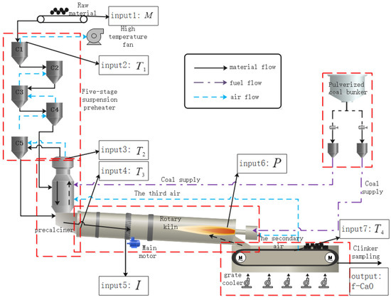
Cement clinker formation involves two key chemical reactions: the decomposition of calcium carbonate (CaCO₃) and the formation of tricalcium silicate (3CaO·SiO₂) [12]. Figure 1 presents a flow diagram to illustrate the key stages and material flow of this calcination process, which are summarized below.

Figure 1. Cement clinker calcination process flow chart.

As shown in Figure 1, the preparation of cement clinker contains three stages: preheating and decomposition, calcination, and clinker cooling. This study delineates the cement clinker calcination process through three pivotal dimensions: material flow, fuel flow, and air flow. Initially, the material flow, integral to the entire process, involves raw materials being conveyed into a suspension preheater where they are uniformly heated by ascending high-temperature airflow, facilitating the preheating phase. The precalciner, serving as a high-temperature reactor, predominantly decomposes calcium carbonate (CaCO₃) into calcium oxide (CaO) and carbon dioxide (CO₂) at approximately 800 °C, achieving a decomposition rate of around 90%. Subsequently, the rotary kiln, operating at temperatures between 1300 °C and 1500 °C, fosters the formation of tricalcium silicate (3CaO·SiO₂), the principal component of cement clinker, through the reaction of CaO with other oxides (Fe₂O₃, Al₂O₃, SiO₂). After the clinker transitions from a solid phase to a liquid phase within the kiln, it enters the grate cooler for rapid cooling. The recovered heat is then returned to the rotary kiln and precalciner for recycling. The pulverized coal bunker supplies the requisite thermal energy for the process, while the high-temperature fan facilitates the recirculation of heat generated during clinker cooling, ensuring the thermal efficiency of the system [13].

2.2. Selection of Auxiliary Variables

To mitigate input noise and improve predictive accuracy, this study employs process mechanism analysis to select seven process variables, each showing a strong correlation with f-CaO content [14]. These variables are drawn from the four-stage process encompassing preheating, decomposition, calcination, and cooling of the clinker. A soft sensor is then developed with f-CaO content as the output. Table 1 summarizes the symbols and units for all variables. The rationale for selecting each is detailed below.

Table 1. Process and quality variables used in the soft sensor model.

Input of the Model		Output of the Model
Raw material preheating	The raw material feeding quantity—$M(\mathrm{t}/\mathrm{h})$	$\mathrm{f-CaO}\left(\mathrm{\%}\right)$
	The outlet temperature of the primary cylinder—$T_1(°\mathrm{C})$
Raw material decomposition	The outlet temperature of $\mathrm{the} \mathrm{precalciner}—T_2(°\mathrm{C})$
Clinker calcining	The negative pressure of kiln head—$P\left(\mathrm{P}\mathrm{a}\right)$
	$\mathrm{The} \mathrm{rotary} \mathrm{kiln} \mathrm{current}—I\left(\mathrm{A}\right)$
	$\mathrm{The} \mathrm{kiln} \mathrm{tail} \mathrm{temperature}{—T}_3(°\mathrm{C})$
Clinker cooling	$\mathrm{The} \mathrm{secondary} \mathrm{air} \mathrm{temperature}—T_4(°\mathrm{C})$

The raw material feeding quantity (M) serves as the benchmark for the production process and directly affects the chemical composition of clinker, thus being treated as a fundamental input variable. Cement manufacturing comprises a series of thermal reactions, primarily the breakdown of CaCO₃ and subsequent oxide recombination. Consequently, the temperature at key equipment stations serves a dual purpose: it indicates operational status and directly governs f-CaO formation [15]. Therefore, the following temperature monitoring variables are selected: Outlet temperature of the primary cylinder ($T_1$, indicating the operating condition of the suspension preheater), Outlet temperature of the precalciner ($T_2$, reflecting the thermal state of the precalciner), Kiln tail temperature ($T_3$, indicating the thermal environment of the rotary kiln tail), and Secondary air temperature ($T_4$, reflecting the heat recovery effect of the grate cooler). The rotary kiln current ($I$) can reflect the load and operational stability within the kiln and is one of the key indicators to measure whether the calcination process is sufficient. The kiln head negative pressure ($P$) is related to the airflow distribution within the kiln, and its stability helps maintain a uniform thermal field within the kiln, promoting the full reaction between CaO and other components. Therefore, it is also included as an input variable [16].

2.3. Data Collection and Preprocessing

The data for this study originates from the actual production database of a cement plant in Hebei Province, China [17]. The acquisition frequency of process variables is 360 times per hour, while the detection frequency of f-CaO content is once per hour. To construct a dataset that comprehensively reflects different production conditions, this paper extracts process variables and f-CaO content data from the database for 60 consecutive days as the basis for modeling and validation.

The process variable values are collected by sensors in actual production conditions. Due to the inherent faults and performance limitations of sensors, the obtained data inevitably contains outliers and noise interference. Furthermore, the numerical ranges of various process variables vary significantly. If not processed uniformly, it may affect the model performance [18]. The specific process variable preprocessing workflow is as follows: Starting with the original process variables, outliers are first identified and eliminated using the 3C criteria. Subsequently, mean filtering is applied to remove noise interference from the data. Next, min-max normalization is employed to standardize the data, ensuring uniform scaling across all variables. The final output consists of cleaned, denoised, and standardized process variables, completing the entire preprocessing pipeline from raw data to directly applicable results [19].

Taking into account the different value ranges between different process variables, this paper uses maximum and minimum standardization to standardize each process variable to keep the value range of each variable within a uniform range. The maximum and minimum standardized formula is shown in Equation (1).

$${x_k}^{\ast }(i)={\displaystyle \frac{x_k(i)-x_{k·\min }}{x_{k·\max }-x_{k·\min }}}$$

(1)

x_k(i) and x_k^*(i) represent the values of the k-th process variable before and after normalization in the i-th sampling, respectively. x_k·max and x_k·min denote the maximum and minimum values, respectively.

Mechanistically, variations in clinker f-CaO content arise from the integrated influence of process variables over time [20]. Accordingly, the model uses historical time-series data of these variables as input to predict the f-CaO level at the subsequent time step. According to the production database records, the acquisition frequency of process variables is 360 times per hour, meaning that 360 time-series points can be obtained per hour. However, considering that process variables usually remain relatively stable on a short time scale, directly using all 360 time-series values as input would result in redundant model structure and excessive computational complexity [21]. To reduce the input dimension and extract more representative temporal features, this paper averages the time-series data of each variable on a per-minute basis (i.e., taking the mean of every consecutive 6 sampling points), thereby compressing the hourly data into 60 feature points. This significantly simplifies the model input while retaining trend information.

Based on the aforementioned discussion, $X=\{M,T_1,T_2,T_3,T_4,I,P\}$ represents the collection of process variables, $X_{\mathrm{tm}}=\{M_{tm},T_{1tm},T_{2tm},T_{3tm},T_{4tm},I_{tm},P_{tm}\}$ indicates the value of all process variables at time tm, and y_N represents the assay value of f-CaO content at the corresponding time. Since the data time span used in this paper is 60 days, the value of N in this paper is 1440, which means that the data set used in this paper contains a total of 1440 time series samples. As illustrated in the data preprocessing description, the samples are constructed by taking time series of process variables of length T and pairing them with the corresponding f-CaO content value [22].

3. Design of TCN Soft Sensor Model Based on Self-Attention Mechanism

This section proposes a soft sensing model based on a Temporal Convolutional Network (TCN) with a self-attention mechanism to achieve online prediction of the f-CaO content in cement clinker. The implementation idea of this model is as follows: Firstly, causal convolution with a dilated structure is utilized to capture the temporal correlation between variables from multi-variable time series inputs and extract their nonlinear temporal features. An attention layer is then applied to dynamically weigh the most influential features for f-CaO prediction. These weighted temporal features are subsequently fed into dense layers, which learn the final nonlinear mapping to estimate f-CaO content in real time [23].

3.1. Temporal Convolutional Network (TCN)

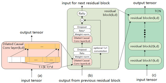
TCN primarily comprises three key components: Causal Convolution, Dilated Convolution, and Residual Connections [24,25,26]. The network structure diagram of TCN can be found in Figure 2.

Figure 2. TCN structure diagram. (a) Input tensor; (b) Dilated causal convolution layer; (c) Output tensor.

The causal convolution operation enforces a strict temporal constraint in TCNs: the activation at any time step t is influenced exclusively by present and past inputs from the preceding layer, thereby preventing any leakage of future information [24]. Let the convolution kernel be F = (f₁, f₂, …, f_K), where K is the kernel size, and the input time series be $X=\{{\mathrm{X}}_1,{\mathrm{X}}_2,\dots {\mathrm{X}}_T\}$. Then the causal convolution operation at time step ${\mathrm{X}}_T$ can be expressed as:

$$F({\mathrm{X}}_T)={\displaystyle \sum _{k=1}^K{f}_k{X}_{T-K+k}}$$

(2)

In Equation (2), $X_{T-K+k}$ represents the multi-dimensional eigenvector at the $(T-K+k)$ moment. $f_K$ represents the corresponding convolution kernel.

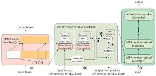
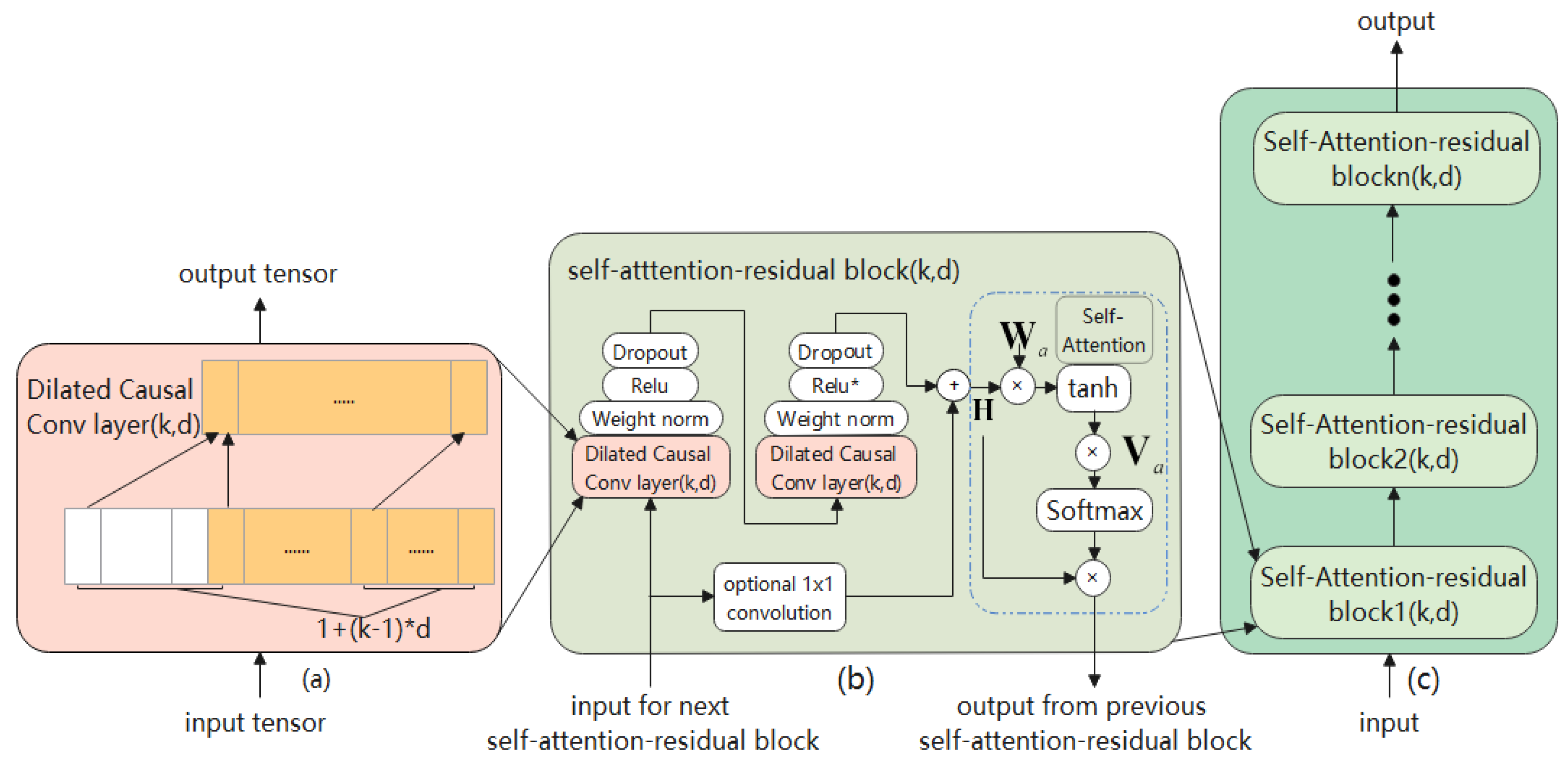
In causal convolutional networks, the expansion of receptive fields primarily relies on increasing the number of network layers (depth) or enlarging the size of convolutional kernels. Both of these methods follow a linear expansion pattern, significantly increasing the computational complexity and parameter scale of the model. When the time series of network input is too long, the network will be too deep, which can be alleviated by introducing dilated convolution [27]. The structural diagram of dilated causal convolution is shown in Figure 3a. The dilated causal convolution operation is shown in Equation (3):

$$F_d({\mathrm{X}}_T)={\displaystyle \sum _{k=1}^K{f}_k{X}_{T-(K-k)d}}$$

(3)

Figure 3. The TCN structure based on self-attention mechanism; (a) Internal structure of a single self-attention-residual block; (b) Stacking of multiple self-attention-residual blocks; (c) Overall model input and output.

In Equation (3), $d$ is the dilated factor, which usually grows exponentially by 2. When the dilated factor d is 1, the dilated causal convolutional network degenerates into a common causal convolutional network.

When the error back propagation algorithm is used to learn network parameters and the network is too deep, the problem of gradient explosion or gradient disappearance will occur. To avoid this problem, TCN introduced an identity mapping of cross-layer connections (implemented by a 1 × 1 convolution) in each of its residual blocks (Figure 3b) [26]. The output of the network is shown in Equation (4):

$$F({\mathrm{X}}_T)=F_d({\mathrm{X}}_T)+X_T$$

(4)

3.2. Self-Attention Mechanism

The core of the self-attention mechanism lies in the model, which can dynamically assess the importance of each feature based on the internal interrelationships of input features through a similarity function, and assign corresponding weights to them. The entire process does not rely on any external information [28]. In a neural network structure, the self-attention mechanism usually realizes this purpose through the network layer. The core formula of the self-attention mechanism is shown in Equations (5) and (6):

$$\mathit{B}=\mathrm{soft}\mathit{max}({\mathit{V}}_a\mathit{tan}h({\mathit{W}}_a\mathit{H}\left)\right)$$

(5)

$$C=BH$$

(6)

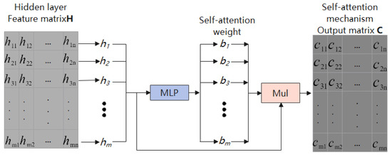
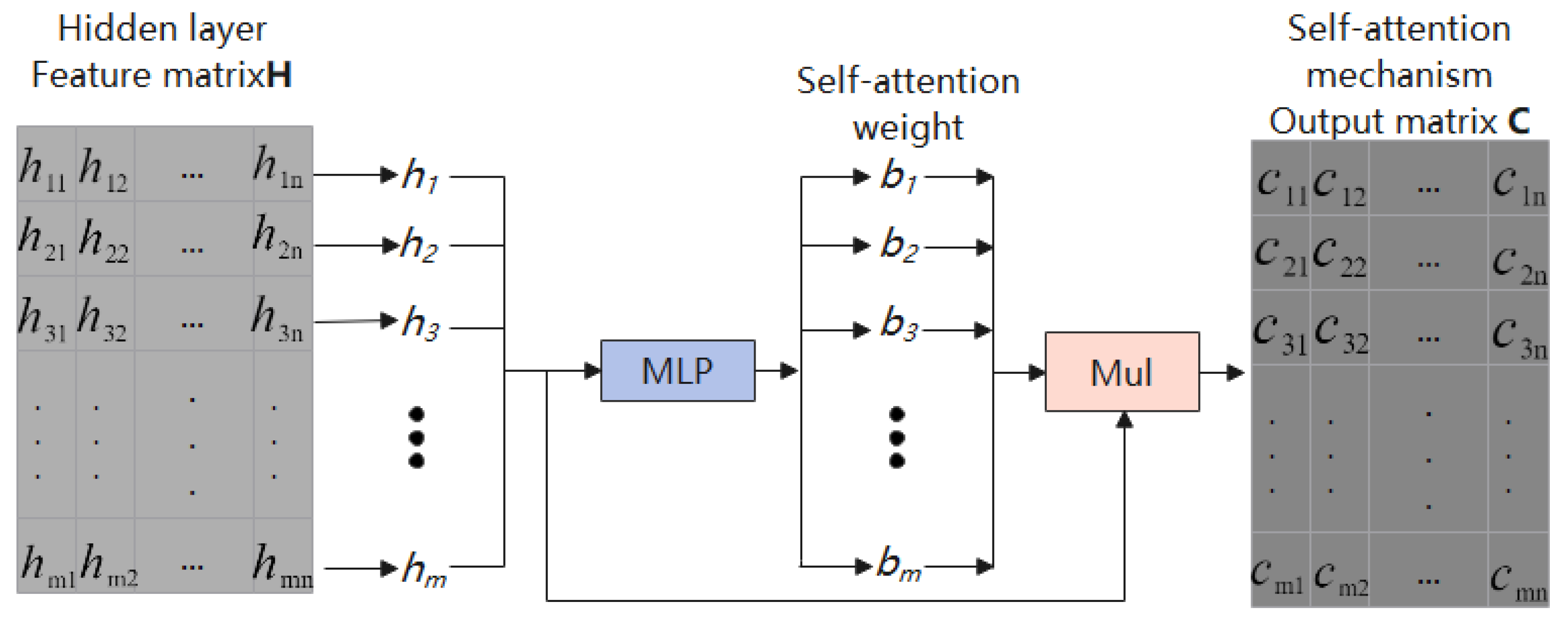
In Equations (5) and (6), $\mathbf{H}$ represents the hidden layer feature matrix, tanh(·) and softmax(·) denote the hyperbolic tangent function and normalized exponential function, respectively, ${\mathbf{W}}_{\mathrm{a}}$ is the weight matrix with the same dimension as $\mathbf{H}$, ${\mathbf{V}}_{\mathrm{a}}$ is the parameter matrix, and $\mathbf{B}$ is the attention weight matrix computed via the softmax function. The matrix $\mathbf{C}$ denotes the output of the hidden layer. Self-attention determines the relevance between different input features using a learned, feed-forward network. The output of this network is transformed into a weight distribution using the softmax function, and then weightedly fused with the input features to obtain the attention-weighted output. The specific calculation process is illustrated in Figure 4 [29].

Figure 4. Schematic diagram of self-attention mechanism realization.

3.3. TCN Structure Based on Self-Attention Mechanism and Real-Time Measurement Model Framework of f-CaO Content in Cement Clinker

The proposed model tackles the coupled temporal effects of process variables on clinker f-CaO by ingesting multivariate temporal data [30]. This data is distilled into deep sequential features, which form the basis for continuous f-CaO content estimation.

While Recurrent Neural Networks (RNNs) have limitations in receptive field size, dilated causal convolution provides extended context coverage for modeling long-range temporal dependencies [31]. Simultaneously, self-attention allows the model to prioritize salient features directly from the input data. Integrating these strengths, we develop a self-attention-enhanced TCN to extract deep nonlinear temporal representations for real-time estimation of clinker f-CaO content. The model architecture is presented in Figure 3.

In the model constructed in this paper, the self-attention mechanism acts on the time series features extracted by the dilated causal convolutional network layer, enhancing the representation ability of nonlinear time series features that significantly affect the output through dynamic weight allocation [32]. This mechanism can effectively suppress the interference of irrelevant information on the model, further improving prediction accuracy. On this basis, by stacking multiple self-attention-residual blocks (k,d), the resulting model learns hierarchical, nonlinear representations from multivariate temporal data and functions as a soft sensor for estimating f-CaO content in cement clinker.

3.3.1. Model Input

The main task of the model input part is to preprocess the original data to make it suitable for the model input. The specific data processing flow has been introduced in Section 2.3. It should be noted that the different waveform curves in the Raw data box represent the measured values of different process variables collected within one hour, and the different colors in the input of the model box represent different process variables after processing (That is, the seven process variables $M$, $T_1$, $T_2$, $T_3$, $T_4$, $I$, $P$ and P selected in Section 2).

3.3.2. Deep Feature Extraction

There is a highly non-linear relationship between the original input data and the output; it is difficult to directly establish a network model to describe the relationship between them. By stacking multiple dilated causal convolution residual blocks based on self-attention mechanism, the deep nonlinear timing features of the input data can be efficiently extracted [33]. In each self-attention-residual block, the input time series is first processed through two layers of dilated causal convolution. Since convolution operations are essentially linear transformations, a ReLU activation function (Equation (7)) is introduced after each convolution layer to enhance the model’s nonlinear expression capability. To suppress overfitting, weight regularization and Dropout techniques are employed in the model [34]. Additionally, to avoid the vanishing gradient problem during gradient descent, an identity mapping formed by 1 × 1 convolution is also introduced into the structure.

$$\mathrm{Re}\mathrm{lu}(x)=\max (0,x)$$

(7)

Owing to the complex interplay among process conditions, it is challenging to pinpoint the influential variables and their precise temporal influence on f-CaO content. Consequently, the nonlinear temporal features learned by dilated causal convolution contribute unevenly to the final output [35]. To further select key features from these, this paper introduces a self-attention mechanism to dynamically redistribute feature weights, thereby enhancing the representation of important temporal features. The specific process is shown in Figure 4. After being processed by multiple stacked self-attention-residual blocks, the final output deep nonlinear temporal feature matrix is denoted as ${\mathbf{C}}^n$, where n represents the number of self-attention-residual blocks used.

3.3.3. Model Output

The model output section employs a fully connected layer to aggregate and transform the nonlinear temporal features extracted by the self-attention-residual block. The input-output relationship of this layer is shown in Equation (8). The f-CaO content is then estimated by applying a linear combination to the outputs of the fully connected layer, and its expression is shown in Equation (9).

$$C^{n+1}=f(W^n{C}^n+{\mathrm{b}}^n)$$

(8)

$${\mathrm{y}}^{\prime }=W^{n+1}{C}^{n+1}+{\mathrm{b}}^{n+1}$$

(9)

The weight matrix Wⁿ and bias vector bⁿ⁺¹ in Equation (8) correspond to the fully connected layer, while Wⁿ⁺¹ and bⁿ⁺¹ in Equation (9) are the parameters of the output layer. In Equation (9), Wⁿ⁺¹ and bⁿ⁺¹ are the weight and bias of the output layer, respectively, while y′ denotes the final predicted value of the f-CaO content by the model.

3.4. Model Training

Our approach employs a deep neural network framework. Outputs are computed via forward propagation, while parameters are updated through error backpropagation [36]. For training, we utilize the mean squared error (MSE, Equation (10)) as the loss function and apply the Adam algorithm for its minimization, enabling efficient parameter learning [37].

$$L={\displaystyle \frac{1}{n}}{\displaystyle \sum _{i=1}^n(y_i-y_i^{\prime }}{)}^2$$

(10)

In Equation (10), $n$ represents the number of training samples in each batch, $y^{\prime }$ is the true value of the sample, and $y^{\prime }$ is the output value of the model.

4. Experimental Results and Discussion

The dataset used in the experiment contains a total of 1320 samples, each representing a 60-min production segment collected under various operating conditions. Crucially, these samples are statistically independent due to the non-overlapping sampling strategy and sufficient gaps between consecutive segments; there is no temporal dependency between different samples. Therefore, random splitting is appropriate for model evaluation. We randomly selected 200 samples from the dataset as the test set and the remaining 1120 samples as the training set. The detailed description of each sample has been given in Section 2. All experiments in this paper were implemented under the TensorFlow 1.12.0 framework and run on a computer equipped with an Intel i5-9400 CPU and 8 GB RAM.

4.1. Evaluation Index of Model Performance

In this paper, we choose $MAE$, $RMSE$, $R^2$ served as the metric. The calculation formula of each evaluation index is shown in Equations (11)–(13):

$$MAE={\displaystyle \frac{1}{m}}{\displaystyle \sum _{i=1}^m\left|y_i^{\prime }-y_i\right|}$$

(11)

$$RMSE=\sqrt{{\displaystyle \frac{{\displaystyle {\sum }_{i=1}^m{(y_u^{\prime }-y_i)}^2}}{m}}}$$

(12)

$$R^2=1-{\displaystyle \frac{{\displaystyle {\sum }_{i=1}^m{(y_i^{\prime }-y_i)}^2}}{{\displaystyle {\sum }_{i=1}^m{(y_i-\overline{y})}^2}}}$$

(13)

In the formula, $y_i^{\prime }$ and $y_i$ represent the true value and the model’s predicted value of the i-th sample, respectively. m denotes the total number of samples in the test set, and $\overline{y}$ represents the mean of the true values in the test set.

RMSE penalizes large errors more heavily, reflecting the overall magnitude of prediction errors, while MAE quantifies the mean absolute deviation between predictions and observations. Lower values for both indicate superior predictive accuracy. The coefficient of determination ($R^2$) measures the proportion of variance in the target variable explained by the model, ranging from 0 to 1. A value approaching 1 denotes a better fit [38].

4.2. Model Hyperparameter Optimization and Structure Optimization

4.2.1. Optimization of Learning Rate (LR)

The learning rate is a crucial hyperparameter in the training process of neural networks, and its value directly affects the optimization behavior of the model’s loss function. When updating parameters using the error backpropagation algorithm, an appropriate learning rate can facilitate the stable convergence of the loss function near the global optimum. In practice, the learning rate must be carefully balanced [39]. A high value may prevent stable convergence by inducing oscillations in the loss landscape, while a low value impedes learning speed and may compel the optimizer to converge to a local minimum. Proper tuning is therefore essential for achieving efficient learning and robust predictive performance [40].

As shown in the experimental results, with different learning rates. When the LR gradually decreases, the model measurement effect gradually becomes better, but when the LR drops from 0.0005 to 0.0001, the performance degrades significantly (MAE increases from 0.09970 to 0.11670, RMSE rises from 0.07851 to 0.12102, and R² drops from 0.73848 to 0.65966). This indicates that the network parameters reach the optimal solution when LR is set to about 0.0005, where the model achieves its best metrics across all evaluation criteria. Finally, we choose to set the LR as 0.0005.

The full progression of testing results demonstrates this trend: at LR = 0.05, the model performs poorly (MAE = 0.20229, RMSE = 0.16421, R² = 0.30796), but performance improves steadily as LR decreases to 0.0005. Beyond this point (LR = 0.0001), all metrics deteriorate, confirming the non-monotonic relationship between LR and model effectiveness [41].

4.2.2. Optimization of Model Network Structure

Although the training speed of a simple network structure is faster, the captured input information is limited. Although the complex network structure can capture more input information, it may cause model overfitting. Therefore, in the process of neural network modeling, the reasonable selection of network structure is a crucial aspect that affects the performance of the model [42].

The network structure of the model in this paper is primarily determined by two aspects: depth and scale. Specifically, depth is controlled by the number of stacked layers n of self-attention-residual blocks; scale depends on the number of filters for dilated causal convolution within each block, the convolution kernel size, and the dilation factor d. The relationship between the dilation factor d and the block index is shown in Equation (14).

$$d=2^n$$

(14)

The meaning of the formula (14) was: if 3 self-attention residual blocks were used, the dilated factors in the 3 self-attention residual blocks were set as 1,2, and 4 in turn.

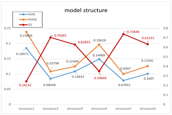
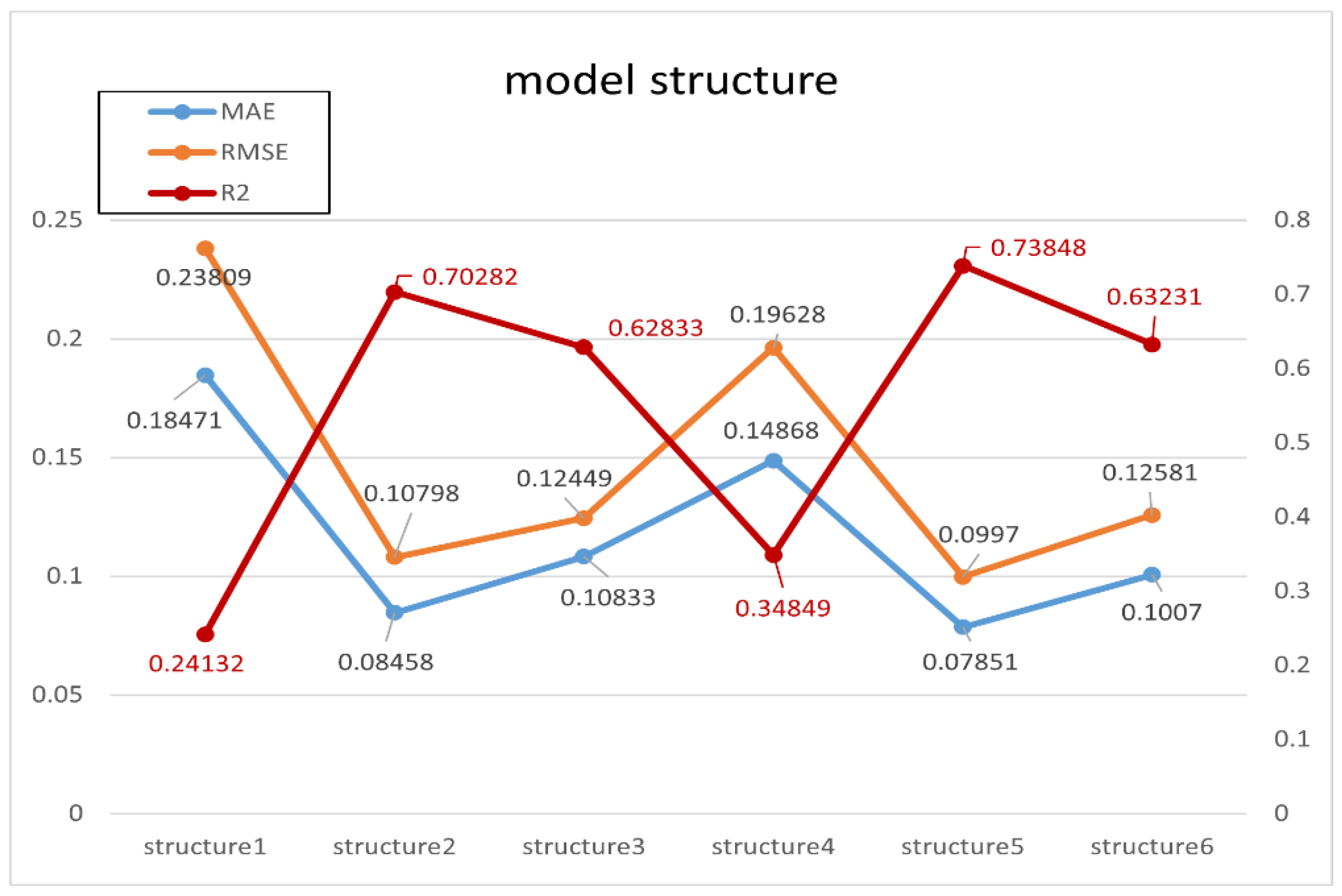
Through many experiments, this paper selected 6 network structures for comparison. The specific network structure parameters are set in Table 2, and the performance index changes of each network structure are shown in Figure 5:

Table 2. Model structure Settings.

Model Structure	$\mathbf{n}$	$\mathbf{Filters}$	$Kernel\_\mathbf{Size}$
structure 1	2	64/32	32/16
structure2	2	64/32	16/8
structure 3	2	64/32	8/4
structure 4	3	64/32/16	32/16/8
structure 5	3	64/32/16	16/8/4
structure 6	3	64/32/16	8/4/2

Figure 5. Model structure optimization experiment.

As shown in Table 2 and Figure 5, in the case of using the same number of self-attention residual blocks and dilated causal convolution kernel, the measurement effect of the model showed a trend of first getting better and then getting worse as the convolution kernel gradually got smaller. This is because the convolution kernel used by the model is too large or too small to extract the correct time series features. It can be shown that setting the appropriate size of the convolution kernel is very important for the measurement accuracy of the model [43]. During the experiment, we also found that when the number of self-attention residual blocks was increased, the measurement effect of the model became better, but at the same time, the complexity of the model became more difficult to optimize [44]. Therefore, in the following experiment, we used structure 5 in Table 2 to compare with other model measurement effects.

4.3. Influence of Time Series of Different Lengths of Process Variables on Model Accuracy

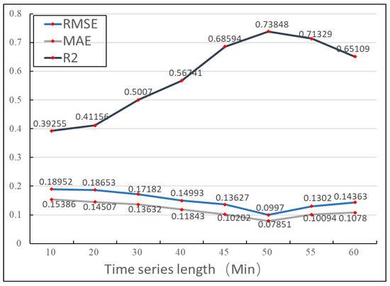
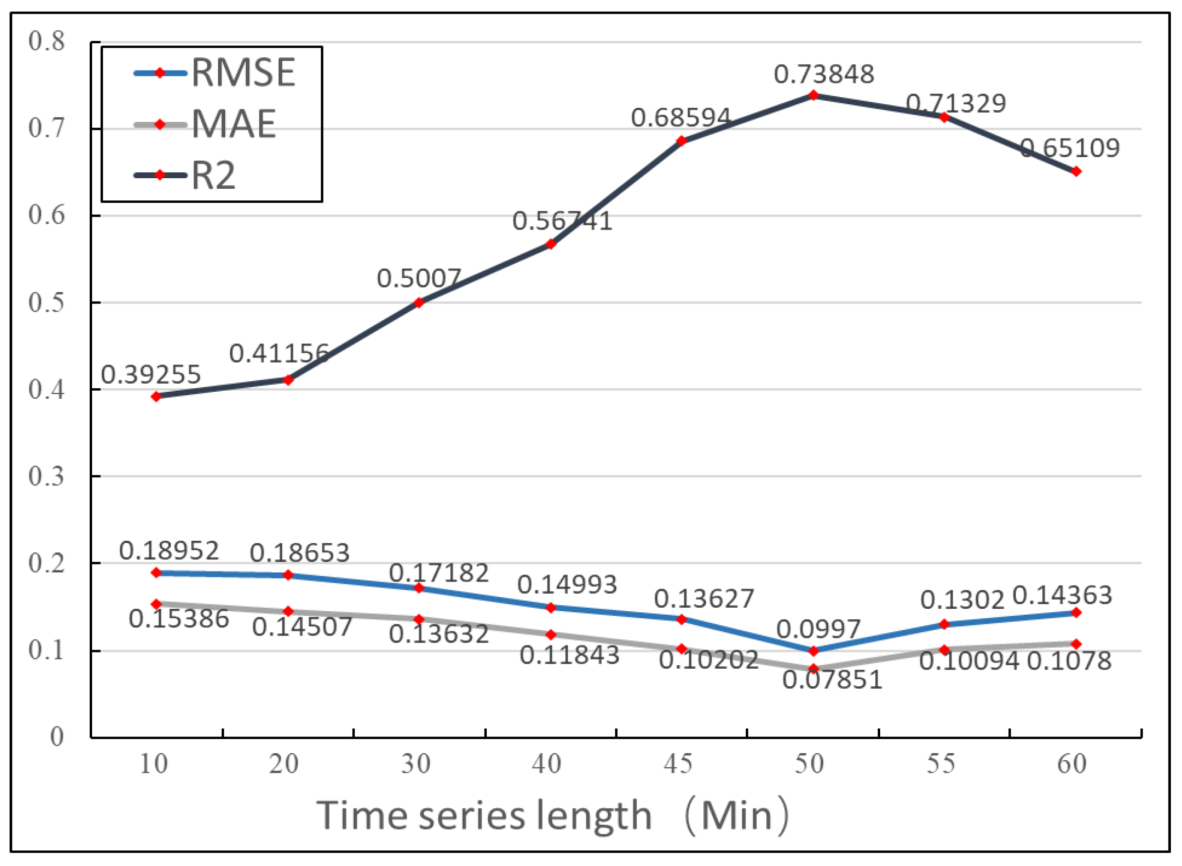
To investigate the influence of different time series lengths of process variables on the model performance, the clinker acquisition time point was selected as the initial reference point [45]. Time series data of varying lengths were then extracted and used as model inputs for experimental evaluation. The experimental results are presented in Figure 6.

Figure 6. Model results at different time series lengths.

In the experiment, process variable time series with lengths of T = 10, 20, 30, 40, 50, and 60 min were tested as model inputs. Preliminary results indicated that the model achieved the highest accuracy when the sequence length was 50 min. To further validate, sequences of 45 min and 55 min were additionally tested. The results are shown in Figure 6: as the sequence length increases, the model accuracy gradually improves, reaching its optimal at 50 min, and then declines. This phenomenon may stem from two factors: within a certain range, longer sequences assist the model in capturing more temporal dependencies, while the attention mechanism effectively filters irrelevant information and reinforces key features; however, when the sequence is excessively long, redundant information may become a burden on the model, adversely affecting its generalization ability [46]. Based on comprehensive experimental results, the input sequence length is ultimately set to 50 min, which provides sufficient and effective temporal information for the measurement of f-CaO content [47].

4.4. Model Comparison Experiment

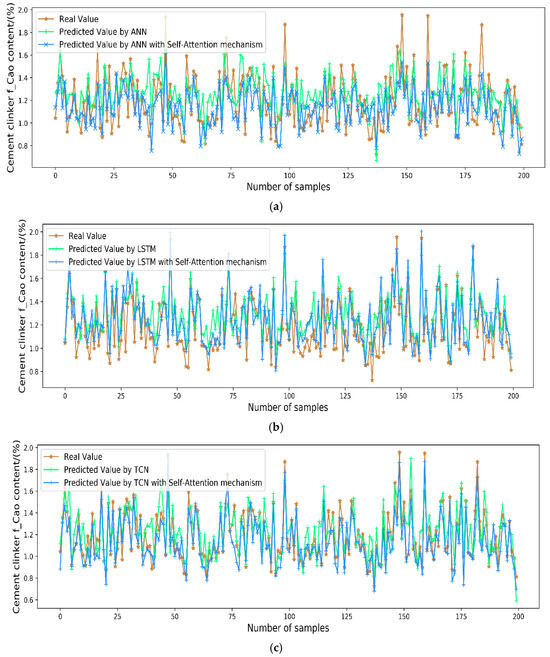
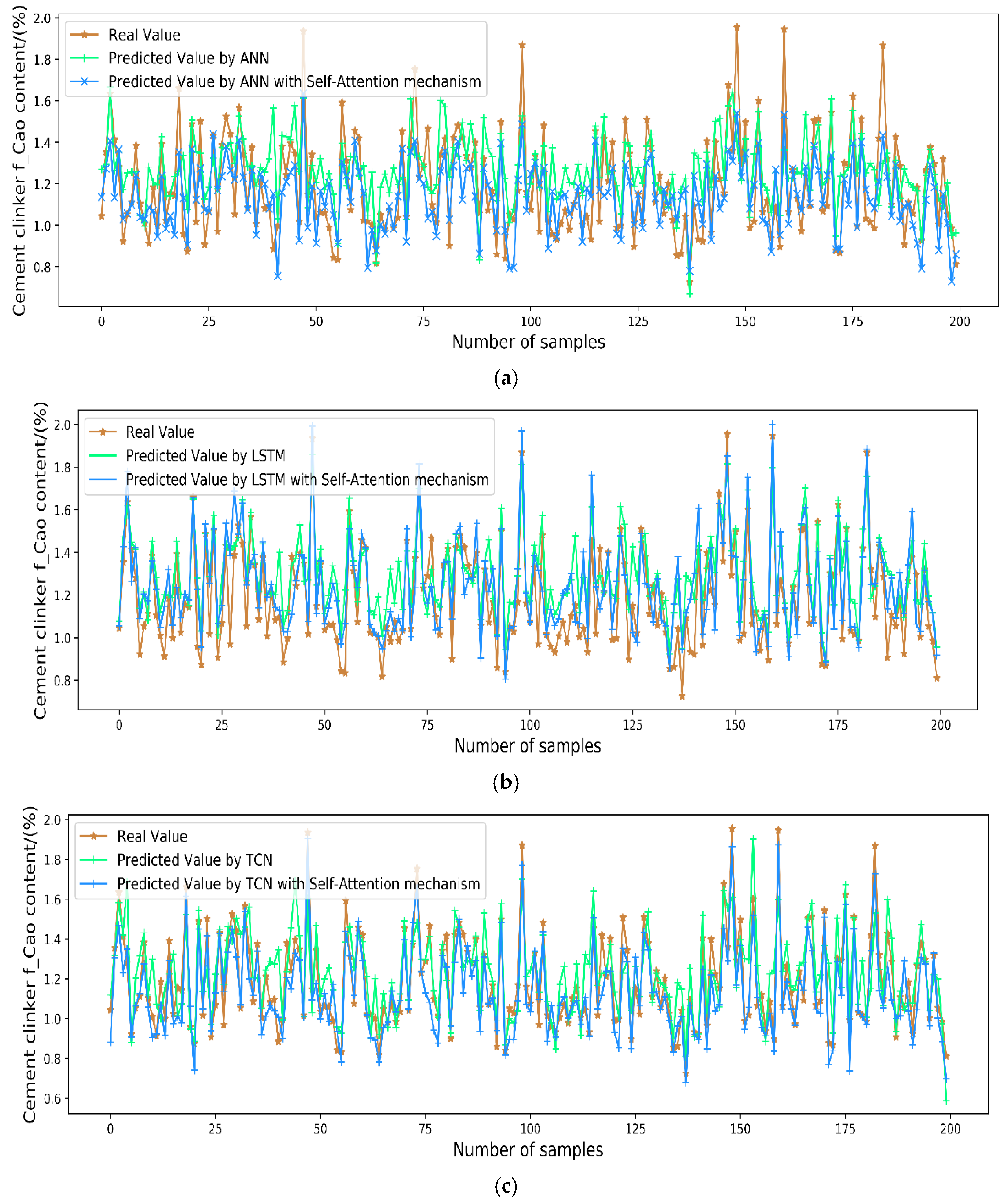
The proposed model was compared with soft sensor models based on ANN and LSTM networks to evaluate its performance. At the same time, in order to reflect the influence of self-attention mechanism on model accuracy, this paper also adds self-attention mechanism to ANN and LSTM networks and carries out comparative experiments [48]. The final output results of each model in the test set are shown in Figure 7.

Figure 7. Comparative Prediction Results of Base Models vs. Self-Attention Enhanced Architectures (ANN, LSTM, TCN). (a) Prediction results of ANN model and ANN model adding self-attention mechanism. (b) Prediction results of LSTM model and LSTM model adding self-attention mechanism. (c) Prediction results of TCN model and TCN model adding self-attention mechanism.

Figure 7a compares the prediction results of the ANN model and its self-attention-enhanced version. It can be observed that the self-attention ANN achieves better alignment with the true values, particularly at peak and trough regions, indicating improved feature extraction capability. Figure 7b presents the comparison between LSTM and self-attention LSTM. The enhanced model shows reduced deviations, demonstrating that the attention mechanism helps the LSTM focus on relevant temporal steps. Figure 7c displays the results of the TCN and self-attention TCN. Among all models, the self-attention TCN exhibits the closest fit to the true f-CaO values, validating the effectiveness of combining TCN’s temporal modeling with dynamic feature weighting.

Based on the experimental results shown in Figure 7, it is evident that the CNN model outperforms the ANN in curve fitting. Specifically, in terms of evaluation metrics, the CNN exhibits a lower RMSE and a higher R² compared to the ANN, indicating that the CNN model possesses superior predictive performance and goodness of fit. This is primarily attributed to the fact that deep learning methods demonstrate stronger capabilities in automatically learning and fitting complex data features when dealing with large-scale data, compared to traditional machine learning methods [49,50].

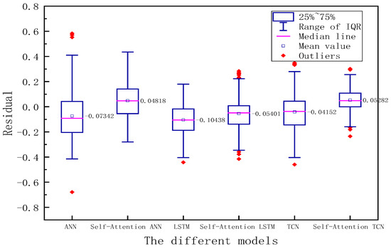
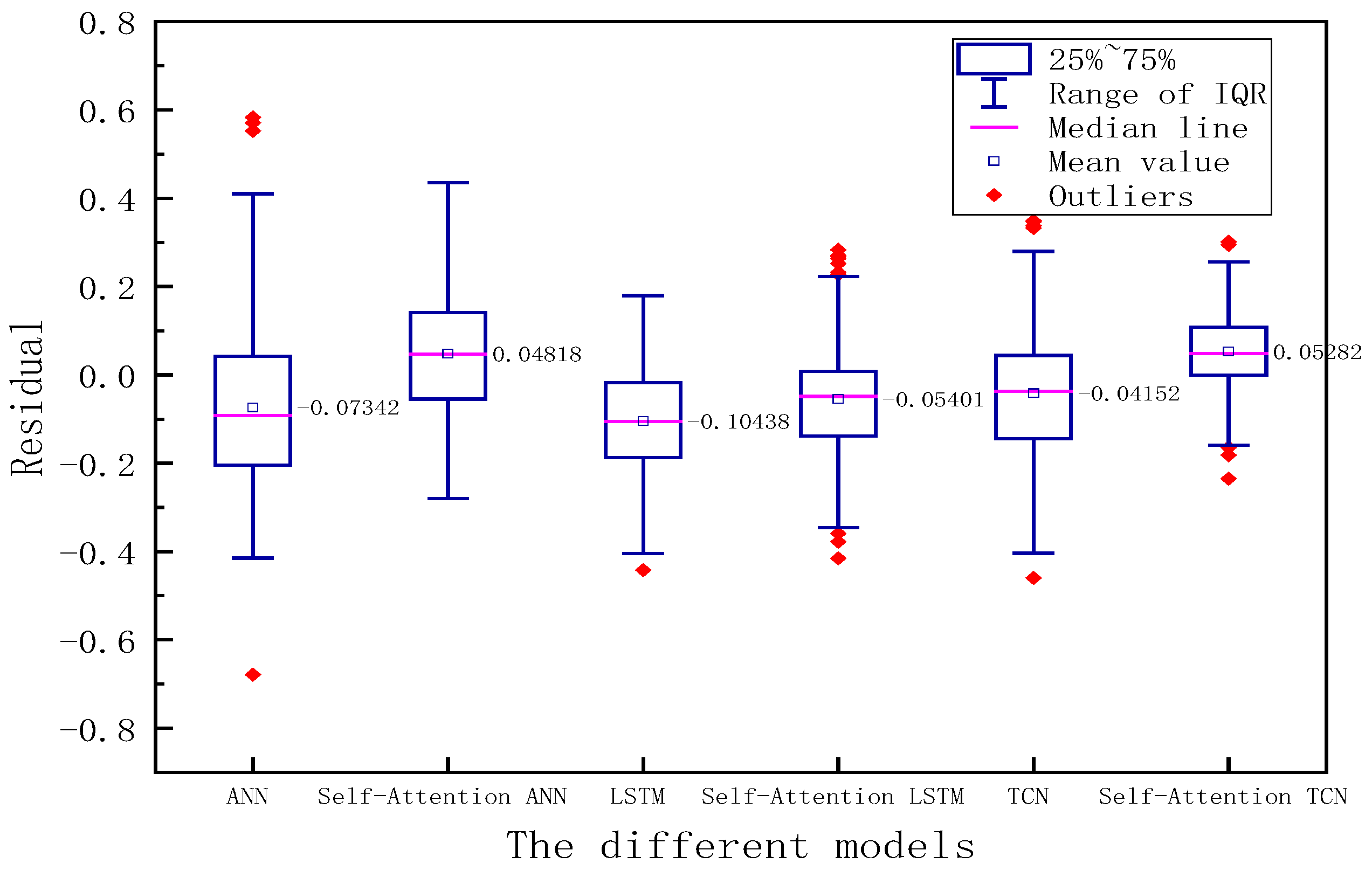
In order to more intuitively reflect the comparison effect between different models, we processed the residual between the real value and the output value of each model, and drew a boxplot for each group of residual results, as shown in Figure 8.

Figure 8. Box plot of residual difference between the predicted results of each model and the true value.

Notably, the self-attention ANN also shows no visible outliers in its residual distribution. This can be attributed to the architectural design of the attention mechanism. Specifically, the self-attention layer computes attention weights via a query-key-value mechanism, dynamically amplifying salient temporal features while suppressing irrelevant noise. The residual connection and layer normalization within each attention block stabilize training and prevent gradient anomalies, leading to more consistent predictions across samples. The stacking of multiple attention blocks progressively refines feature representations, and the inclusion of global statistics provides additional robustness. Collectively, these factors effectively suppress extreme prediction errors, resulting in a compact residual distribution without outliers.

To evaluate error distribution and stability, Figure 8 compares model residuals via boxplots [51]. The proposed self-attention TCN exhibits the narrowest interquartile range and fewest outliers, indicating superior prediction stability and reliability. Quantitative metrics further validate its dominance: it achieves the lowest RMSE (0.0785 vs. 0.1197 for TCN, 0.1302 for LSTM, and 0.1588 for ANN) [52]. The integration of self-attention amplifies TCN’s inherent strength in capturing long-range dependencies, yielding a 34.3% RMSE reduction compared to the base TCN, significantly outperforming LSTM’s 17.0% improvement. This synergy between self-attention’s dynamic feature weighting and TCN’s temporal modeling capability effectively addresses nonlinear challenges in industrial time-series data, particularly under noisy and coupled conditions, establishing a robust framework for soft sensing applications [53].

5. Conclusions

The f-CaO content is a key indicator for measuring the quality of cement clinker, but unlike parameters such as temperature and pressure, it is difficult to directly measure online through hardware sensors. Consequently, soft sensors based on data-driven approaches have become widely used in this context [54]. Our work introduces a TCN that integrates a self-attention mechanism to predict the f-CaO content in cement clinker. The model is designed to capture complex, nonlinear dynamics in multivariate temporal data, thereby reflecting how process variables cumulatively influence f-CaO levels [55].

The experimental results show that the proposed TCN self-attention model can effectively extract key temporal features from multivariate time series, and its predictive performance is superior to traditional methods. This study not only provides a robust soft sensing framework for industrial process modeling, but also offers feasible ideas for real-time quality monitoring [56]. Future work will focus on the online deployment of this model and its further integration with other advanced learning structures to continuously improve practical application effectiveness [57].

To measure the f-CaO content, our model integrates nonlinear time series features through a fully connected network. Additionally, the model’s parameters and structure were fine-tuned through extensive experimentation to achieve optimal performance. Finally, the effectiveness of the proposed model was validated by comparing it with other network models, confirming its superior accuracy and robustness [58].

References

- Kano, M.; Fujiwara, K. Virtual sensing technology in process industries: Trends and challenges revealed by recent industrial applications. J. Chem. Eng. Jpn. 2013, 46, 1–17. [Google Scholar] [CrossRef] [Scilit]
- Liu, X.; Jin, J.; Wu, W.; Herz, F. A novel support vector machine ensemble model for estimation of free lime content in cement clinkers. ISA Trans. 2020, 99, 479–487. [Google Scholar] [CrossRef] [Scilit] [PubMed]
- Qiao, J.; Fang, Z.; Chai, T. LS-SVR-based soft sensor model for cement clinker calcination process. In Proceedings of the 2010 International Conference on Measuring Technology and Mechatronics Automation, Changsha City, China, 13–14 March 2010; pp. 591–594. [Google Scholar]
- Shi, X.; Xiong, W. Adaptive ensemble learning strategy for semi-supervised soft sensing. J. Frankl. Inst. 2020, 357, 3753–3770. [Google Scholar] [CrossRef] [Scilit]
- Wang, L.; Zhao, Q.; Tang, X.; Li, Y.; Chen, J.; Zhao, Y. Robust soft sensor development using adversarial autoencoders under data uncertainty. J. Process Control 2021, 107, 1–12. [Google Scholar]
- Xie, F.; Zhang, P.; Jiang, T.; She, J.; Shen, X.; Xu, P.; Guan, Z. Lesion segmentation framework based on convolutional neural networks with dual attention mechanism. Electronics 2021, 10, 3103. [Google Scholar] [CrossRef] [Scilit]
- Yao, L.; Ge, Z. Deep learning of semisupervised process data with hierarchical extreme learning machine and soft sensor application. IEEE Trans. Ind. Electron. 2018, 65, 1490–1498. [Google Scholar] [CrossRef] [Scilit]
- Li, X.; Zhang, W.; Wang, Y.; Chen, H.; Liu, Z. Digital twin-driven thermal efficiency optimization in cement rotary kilns via hybrid physics-guided neural networks. Energy Convers. Manag. 2022, 267, 115941. [Google Scholar]
- Chen, Z.; Li, M.; Wang, Y.; Zhang, H.; Liu, J. Multimodal deep learning with spatiotemporal attention for industrial quality prediction. IEEE Trans. Ind. Inform. 2023, 19, 1234–1245. [Google Scholar]
- Yuan, X.; Ge, Z.; Huang, B.; Song, Z. A probabilistic just-in-time learning framework for soft sensor development with missing data. IEEE Trans. Control Syst. Technol. 2017, 25, 1124–1132. [Google Scholar] [CrossRef] [Scilit]
- Mikulčić, H.; Vujanović, M.; Fidaros, D.K.; Priesching, P.; Minić, I.; Tatschl, R.; Duić, N.; Stefanović, G. The application of CFD modelling to support the reduction of CO2 emissions in cement industry. Energy 2012, 45, 464–473. [Google Scholar] [CrossRef] [Scilit]
- Liu, X.; Xu, X.; Wu, W.; Herz, F.; Specht, E. A simplified model to calculate the power draw for material movement in industrial rotary kilns. Powder Technol. 2016, 301, 1294–1298. [Google Scholar] [CrossRef] [Scilit]
- Pani, A.K.; Mohanta, H.K. A hybrid soft sensing approach of a cement mill using principal component analysis and artificial neural networks. In Proceedings of the 2013 3rd IEEE International Advance Computing Conference (IACC), Ghaziabad, India, 22–23 February 2013; pp. 713–718. [Google Scholar]
- Dai, J.; Chen, N.; Yuan, X.; Gui, W.; Luo, L. Temperature prediction for roller kiln based on hybrid first-principle model and data-driven MW-DLWKPCR model. ISA Trans. 2020, 98, 403–417. [Google Scholar] [CrossRef] [Scilit]
- Farizhandi, A.A.K.; Zhao, H.; Lau, R. Modeling the change in particle size distribution in a gas-solid fluidized bed due to particle attrition using a hybrid artificial neural network-genetic algorithm approach. Chem. Eng. Sci. 2016, 155, 210–220. [Google Scholar] [CrossRef] [Scilit]
- Yao, L.; Jiang, X.; Huang, G.; Qian, J.; Shen, B.; Xu, L.; Ge, Z. Virtual sensing f-CaO content of cement clinker based on incremental deep dynamic features extracting and transferring model. IEEE Trans. Instrum. Meas. 2021, 70, 1–10. [Google Scholar] [CrossRef] [Scilit]
- Liu, Y.; Wu, Q.-Y.; Chen, J. Active selection of informative data for sequential quality enhancement of soft sensor models with latent variables. Ind. Eng. Chem. Res. 2017, 56, 4804–4817. [Google Scholar] [CrossRef] [Scilit]
- Yuan, X.; Huang, B.; Wang, Y.; Yang, C.; Gui, W. Deep learning-based feature representation and its application for soft sensor modeling with variable-wise weighted SAE. IEEE Trans. Ind. Inform. 2018, 14, 3235–3243. [Google Scholar] [CrossRef] [Scilit]
- Aghili, F.; Su, C.-Y. Robust relative navigation by integration of ICP and adaptive Kalman filter using laser scanner and IMU. IEEE/ASME Trans. Mechatron. 2016, 21, 2015–2026. [Google Scholar] [CrossRef] [Scilit]
- Mariani, S.; Rendu, Q.; Urbani, M.; Sbarufatti, C. Causal dilated convolutional neural networks for automatic inspection of ultrasonic signals in non-destructive evaluation and structural health monitoring. Mech. Syst. Signal Process. 2021, 146, 106989. [Google Scholar] [CrossRef] [Scilit]
- Zhang, Y.; Li, X.; Wang, Y.; Liu, Z.; Chen, H. Deep hybrid neural network with attention mechanism for cement clinker quality prediction. Control Eng. Pract. 2022, 118, 104456. [Google Scholar]
- Zhao, J.; Chen, J.; Meng, X.; Zhai, J. Maximizing bi-mutual information of features for self-supervised deep clustering. Adv. Comput. Intell. 2021, 1, 3. [Google Scholar] [CrossRef] [Scilit]
- Zheng, J.; Zhao, L.; Du, W. Hybrid model of a cement rotary kiln using an improved attention-based recurrent neural network. ISA Trans. 2022, 128, 181–192. [Google Scholar] [CrossRef] [Scilit] [PubMed]
- Bai, S.; Kolter, J.Z.; Koltun, V. An empirical evaluation of generic convolutional and recurrent networks for sequence modeling. arXiv 2018, arXiv:1803.01271. [Google Scholar] [CrossRef] [Scilit]
- Lea, C.; Flynn, M.D.; Vidal, R.; Reiter, A.; Hager, G.D. Temporal convolutional networks for action segmentation and detection. In Proceedings of the IEEE Conference on Computer Vision and Pattern Recognition, Honolulu, HI, USA, 21–26 July 2017; pp. 156–165. [Google Scholar]
- He, K.; Zhang, X.; Ren, S.; Sun, J. Deep residual learning for image recognition. In Proceedings of the IEEE Conference on Computer Vision and Pattern Recognition, Las Vegas, NV, USA, 27–30 June 2016; pp. 770–778. [Google Scholar]
- Yu, F.; Koltun, V. Multi-scale context aggregation by dilated convolutions. In Proceedings of the International Conference on Learning Representations, San Juan, PR, USA, 2–4 May 2016. [Google Scholar]
- Vaswani, A.; Shazeer, N.; Parmar, N.; Uszkoreit, J.; Jones, L.; Gomez, A.N.; Kaiser, Ł.; Polosukhin, I. Attention is all you need. In Proceedings of the Advances in Neural Information Processing Systems, Long Beach, CA, USA, 4–9 December 2017; pp. 5998–6008. [Google Scholar]
- Wang, X.; Girshick, R.; Gupta, A.; He, K. Non-local neural networks. In Proceedings of the IEEE Conference on Computer Vision and Pattern Recognition, Salt Lake City, UT, USA, 18–22 June 2018; pp. 7794–7803. [Google Scholar]
- Zhao, Y.; Ding, B.; Zhang, Y.; Yang, L.; Hao, X. Online cement clinker quality monitoring: A soft sensor model based on multivariate time series analysis and CNN. ISA Trans. 2021, 108, 246–257. [Google Scholar] [CrossRef] [Scilit] [PubMed]
- Guo, R.; Liu, H. A hybrid mechanism- and data-driven soft sensor based on the generative adversarial network and gated recurrent unit. IEEE Sens. J. 2021, 21, 18267–18278. [Google Scholar] [CrossRef] [Scilit]
- Hu, X.; Geng, Z.; Han, Y.; Huang, W.; Chen, K.; Xie, F. Novel soft sensor model based on spatio-temporal attention. In Proceedings of the 2021 International Joint Conference on Neural Networks (IJCNN), Shenzhen, China, 18–22 July 2021; pp. 1–8. [Google Scholar]
- Zhou, J.-Y.; Yang, C.-H.; Wang, X.-L.; Cao, S.-Y. A soft sensor modeling framework embedded with domain knowledge based on spatio-temporal deep LSTM for process industry. Eng. Appl. Artif. Intell. 2023, 117, 105552. [Google Scholar] [CrossRef] [Scilit]
- Chen, X.; Hu, Y.; Liu, C.; Chen, A.; Chi, Z. Dynamic spatiotemporal graph network based on multi-level feature interaction for sinter TFe prediction. J. Process Control 2025, 125, 103–115. [Google Scholar]
- Srivastava, N.; Hinton, G.; Krizhevsky, A.; Sutskever, I.; Salakhutdinov, R. Dropout: A simple way to prevent neural networks from overfitting. J. Mach. Learn. Res. 2014, 15, 1929–1958. [Google Scholar]
- Brunner, V.; Siegl, M.; Geier, D.; Becker, T. Biomass soft sensor for a fed-batch process based on phase detection and hybrid modeling. Biotechnol. Bioeng. 2020, 117, 1866–1875. [Google Scholar] [CrossRef] [Scilit]
- Rumelhart, D.E.; Hinton, G.E.; Williams, R.J. Learning representations by back-propagating errors. Nature 1986, 323, 533–536. [Google Scholar] [CrossRef] [Scilit]
- Kingma, D.P.; Ba, J. Adam: A method for stochastic optimization. In Proceedings of the International Conference on Learning Representations, San Diego, CA, USA, 7–9 May 2015. [Google Scholar]
- Chicco, D.; Warrens, M.J.; Jurman, G. The coefficient of determination R-squared is more informative than SMAPE, MAE, MAPE, MSE and RMSE in regression analysis evaluation. PeerJ Comput. Sci. 2021, 7, e623. [Google Scholar] [CrossRef] [Scilit]
- Smith, L.N. Cyclical learning rates for training neural networks. In Proceedings of the 2017 IEEE Winter Conference on Applications of Computer Vision (WACV), Santa Rosa, CA, USA, 24–31 March 2017; pp. 464–472. [Google Scholar]
- You, Y.; Gitman, I.; Ginsburg, B. Large batch training of convolutional networks. arXiv 2017, arXiv:1708.03888. [Google Scholar] [CrossRef] [Scilit]
- Loshchilov, I.; Hutter, F. SGDR: Stochastic gradient descent with warm restarts. In Proceedings of the International Conference on Learning Representations, Toulon, France, 24–26 April 2017. [Google Scholar]
- Goodfellow, I.; Bengio, Y.; Courville, A. Deep Learning; MIT Press: Cambridge, MA, USA, 2016. [Google Scholar]
- Krizhevsky, A.; Sutskever, I.; Hinton, G.E. ImageNet classification with deep convolutional neural networks. In Advances in Neural Information Processing Systems; Curran Associates, Inc.: Red Hook, NY, USA, 2012; pp. 1097–1105. [Google Scholar]
- He, K.; Zhang, X.; Ren, S.; Sun, J. Identity mappings in deep residual networks. In European Conference on Computer Vision; Springer: Berlin/Heidelberg, Germany, 2016; pp. 630–645. [Google Scholar]
- Zhao, Y.; Wu, R.; Zhang, S.; Qu, H.; Hao, X. Soft sensor modeling of cement clinker quality: A novel timing matching technique and data decoupling approach. Meas. Sci. Technol. 2023, 34, 045013. [Google Scholar] [CrossRef] [Scilit]
- Hochreiter, S.; Schmidhuber, J. Long short-term memory. Neural Comput. 1997, 9, 1735–1780. [Google Scholar] [CrossRef] [Scilit] [PubMed]
- Liu, G.; Xie, S.; Hao, X.; Yang, M.; Yang, X.; Xu, X.; Guo, H. Dynamic multi-objective optimization method for production index of cement clinker firing process based on collaborative prediction strategy. Eng. Appl. Artif. Intell. 2025, 129, 105678. [Google Scholar] [CrossRef] [Scilit]
- Xu, M.; Liu, H.; Yang, H. A deep learning based multi-block hybrid model for bike-sharing supply-demand prediction. IEEE Access 2020, 8, 113467–113477. [Google Scholar] [CrossRef] [Scilit]
- Cortes, C.; Vapnik, V. Support-vector networks. Mach. Learn. 1995, 20, 273–297. [Google Scholar] [CrossRef] [Scilit]
- LeCun, Y.; Bengio, Y.; Hinton, G. Deep learning. Nature 2015, 521, 436–444. [Google Scholar] [CrossRef] [Scilit]
- Tukey, J.W. Exploratory Data Analysis; Addison-Wesley: Reading, MA, USA, 1977. [Google Scholar]
- Hao, X.; Dang, H.; Zhang, Y.; Liu, L.; Huang, G.; Zhang, Y.; Liu, J. SSP-WGAN-based data enhancement and prediction method for cement clinker f-CaO. IEEE Sens. J. 2022, 22, 12034–12044. [Google Scholar] [CrossRef] [Scilit]
- Zhao, Y.; Han, Y.; Zhang, C.; Ding, B.; Hao, X. A novel integrated soft sensing model for online cement clinker quality monitoring based on fuzzy fine-grained classification. Appl. Soft Comput. 2024, 153, 111–123. [Google Scholar] [CrossRef] [Scilit]
- Qin, S.J.; Chiang, L.H. Advances and opportunities in machine learning for process data analytics. Comput. Chem. Eng. 2019, 126, 465–473. [Google Scholar] [CrossRef] [Scilit]
- Ge, Z.; Song, Z.; Gao, F. Review of recent research on data-based process monitoring. Ind. Eng. Chem. Res. 2013, 52, 3543–3562. [Google Scholar] [CrossRef] [Scilit]
- Kadlec, P.; Gabrys, B.; Strandt, S. Data-driven soft sensors in the process industry. Comput. Chem. Eng. 2009, 33, 795–814. [Google Scholar] [CrossRef] [Scilit]
- Shang, C.; Yang, F.; Huang, D.; Lyu, W. Data-driven soft sensor development based on deep learning technique. J. Process Control 2014, 24, 223–233. [Google Scholar] [CrossRef] [Scilit]
Disclaimer/Publisher’s Note: The statements, opinions and data contained in all publications are solely those of the individual author(s) and contributor(s) and not of MDPI and/or the editor(s). MDPI and/or the editor(s) disclaim responsibility for any injury to people or property resulting from any ideas, methods, instructions or products referred to in the content. |
© 2026 by the authors. Licensee MDPI, Basel, Switzerland. This article is an open access article distributed under the terms and conditions of the Creative Commons Attribution (CC BY) license.